Optimizing Quantum Walk Search on a Reduced Uniform Complete Multi-Partite Graph

Abstract

In a recent work by Novo et al. (Sci. Rep. $\mathbf{5}$, 13304, 2015), the invariant subspace method was applied to the study of continuous-time quantum walk (CTQW). The method helps to reduce a graph into a simpler version that allows more transparent analyses of the quantum walk model. In this work, we adopt the aforementioned method to investigate the optimality of a quantum walk search of a marked element on a uniform complete multi-partite graph. We formulate the eigenbasis that would facilitate the transport between the two lowest energy eigenstates and demonstrate how to set the appropriate coupling factor to preserve the optimality.

1 Introduction

Various quantum computational frameworks, such as Quantum Circuit Model [nielsen2002quantum], Topological Quantum Computation [freedman2003topological], Adiabatic Quantum Computation (AQC) [farhi2000quantum], Quantum Walk (QW) [aharonov1993quantum, farhi1998quantum], Resonant Transition Based Quantum Computation (RTBQC) [chiang2017resonant] and Measurement Based Quantum Computation (MBQC) [briegel2009measurement] have been proposed to attack problems that are considered extremely difficult for classical computers. Notable successes include the inventions of Shor’s factoring algorithm and Grover’s search algorithm, which manifest indisputable enhancement over all known classical algorithms designed for the same purpose. Among the proposed quantum computational frameworks above, quantum walk models are certainly among the most heavily supported. They provide a natural framework for tackling spatial search problems such as implementing the Grover’s search algorithm [grover1996fast]. In addition, they are central to quantum algorithms [childs2004spatial, childs2003exponential] created to tackle other computationally hard problems, such as graph isomorphism[berry2011two, gamble2010two, douglas2008classical], network analysis and navigation [berry2010quantum, sanchez2012quantum], and quantum simulation [lloyd1996universal, berry2009black, schreiber20122d], even including certain aspects of complex biological processes [engel2007evidence, rebentrost2009environment]. Furthermore, due to the simple physics principle behind quantum walk models, various efforts have been made to establish a better understanding of quantum walk models by relating to other major quantum computational frameworks or explore novel approaches to exploit quantum walks to perform a greater variety of tasks [childs2009universal, du2003experimental, wong2016irreconcilable, sanders2017qwchimera, kitagawa_12, zanetti_14].

Quantum walks can be formulated in both discrete time [aharonov1993quantum] and continuous time [farhi1998quantum] versions. In this work, we focus on the study of continuous-time quantum walk (CTQW), not only because it offers a simpler physical picture but also it is less challenging to perform CTQW experiments in comparison to their discrete-time counterparts. Furthermore, if implementing CTQW in a quantum circuit model, robust quantum computations could be attained due to the availability of fault tolerance and error corrections. Based on these motivations, we set out to investigate how to optimize CTQW searches on a uniform complete multi-partite graph. Although uniform complete multi-partite graphs constitute just a subset of all possible graphs, they include some of the most important examples, such as complete graphs, complete bipartite graphs and star graphs which will be further elaborated in section LABEL:sect:Examples, in applications of quantum walks to computations.

In this work, we adopt the invariant subspace method from Ref.[novo2015systematic], which allows us to perform a dimensionality reduction to simplify the analyses of CTQW on a uniform complete multi-partite graph. In short, the key is to transform the original graph to a much simpler structure yet retain pertinent properties that we would like to investigate, such as the optimality of a quantum walk search. In this way, the analysis becomes more transparent and the dynamics of the walker can be more intuitively understood on an abstract level. Throughout the text, we also refer to a multi-partite graph as a $P$-partite with a slight twist on the standard notation. The difference is that the whole graph has actually $P+1$ partitions where the extra one partition is the partition that contains the solution (marked vertex).

The contribution from this work is as follows. By applying the systematic dimensionality reduction technique via Lanczos algorithm, we extend the applicable graphs from complete graphs, complete bipartite graphs and star graphs [novo2015systematic] to uniform complete multi-partite graphs. We extend a reduction scheme to transform an arbitrary $N$ by $N$ adjacency matrix $H_{a}$ of a uniform complete multi-partite graph into a 3 by 3 reduced Hamiltonian that has fast transport between its two lowest eigenenergy states. We further parameterize the coupling factor based on the configuration of a given uniform complete multi-partite graph to keep the CTQW search optimal.

The remainder of the article is organized as the following. In section 2, we first summarize the notion of invariant subspace discussed in [novo2015systematic]. In section 3, we apply the method to analyze optimality of uniform complete P-partite graphs. In section LABEL:sect:HamilSearchG we further develop theorems to show (a) how to choose the correct coupling factor based on the given parameters (configuration) on a reduced graph and (b) the optimality is preserved once transformed back to the original graph. By adding additional constraints to our finding, we recover many useful examples such as complete graphs, star graphs and complete bipartite graphs in section LABEL:sect:Examples. The reduced Hamiltonian is slightly different for each of these three cases because there are transitions among partitions that behave differently for each case. Finally in section LABEL:sect:discussion, we draw our conclusion.

2 Invariant Subspace of a Quantum Walk

Continuous-time quantum walk on a graph is a quantum dynamical process governed by a tight binding Hamiltonian. Given a graph $G(V,E)$ (characterized by the vertex set V and the edge set E), one constructs the corresponding CTQW model by first defining a Hilbert space with state $|i\rangle$ from node $i$ in $V$. In most cases and in this study, the tight binding Hamiltonian is defined as

$$\langle i|H_{a}|j\rangle=\left\{\begin{array}[]{cc}1,\,\,(i,j)\in E\\ 0.\,\,\text{otherwise}\end{array}\right.$$ (3)

Alternatively, $H_{a}$ is simply called the adjacency matrix of the unweighted graph.

A time-evolved wave function on the graph is given by

$$|\psi(t)\rangle = \exp(-iH_{a}t)|\psi(0)\rangle$$ (4)

$$= \sum_{n=0}^{\infty}\frac{(it)^{n}}{n!}H_{a}^{n}|\psi(0)\rangle$$

$$= \sum_{n=0}^{\infty}\frac{(it)^{n}}{n!}|\psi^{(n)}(0)\rangle.$$

Due to the finite dimensionality of the Hilbert space, the number of independent states $\mathcal{I}(H_{a},|\psi(0)\rangle)\equiv span\{|\psi^{(n)}(0)\rangle=H^{n}_{a}|\psi(0)\rangle\}$ generated from the unitary dynamics (equivalent to repeated actions of the Hamiltonian) is bounded by $|V|$, the cardinality of vertex set. Following Ref. [novo2015systematic], we designate $\mathcal{I}(H_{a},|\psi(0)\rangle)$ as the invariant subspace with respect to $|\psi(0)\rangle$. When the Hamiltonian features certain symmetries, the invariant subspace could be much smaller than $|V|$. Let $\mathcal{P}$ be the projection onto $\mathcal{I}(H_{a},|\psi(0)\rangle)$, one finds the same unitary dynamics can be generated by an effective Hamiltonian $\mathcal{P}H_{a}\mathcal{P}=H_{ra}$, i.e $\exp(-iH_{a}t)|\psi(0)\rangle=\exp(-iH_{ra}t)|\psi(0)\rangle$ for all time $t$. In the following sections, we should apply this concept to identify the invariant subspace of a marked element $|w\rangle$ in multi-partite graphs and study the properties of CTQW in the reduced Hilbert space with an effective Hamiltonian $H_{ra}$.

3 Search in Uniform Complete Multi-Partite Graphs

In this section, we first describe the procedures it requires to perform the dimentionality redution and CTQW construction based on the reduced dimension and the chosen coupling factor $\gamma$. We then further show that CTQW based on the chosen coupling factor $\gamma$ will still preserve its quadratic speed-up, i.e. remaining optimal. The reduction and coupling factor $\gamma$ determination process is as the following.

Algorithm 1 Mechanism: Dimensionality Reduction and Coupling Factor Determination

0:  A UCPG G of arbitrary size with one marked element $|\omega\rangle$

0:  $|\omega\rangle$ can be found efficiently by CTQW.

  Start of process

  $\bullet$ Dimensionality Reduction: Construct the reduced 3 by 3 Hamiltonian $H_{ra}$ by use of Lanczos algorithm on the $N$ by $N$ adjacency matrix $H_{a}$ based on a UCPG G

  $\bullet$ Hamiltonian Construction: Construct CTQW Hamiltonian $H_{seek}=-\gamma H_{ra}-|\omega\rangle\langle\omega|$.

  $\bullet$ Basis Change: Express $H_{seek}=H^{(0)}+H^{(1)}$ in the eigenbasis $(|\omega\rangle,|e_{1}\rangle,|e_{2}\rangle)$ of $H^{(0)}$ by applying perturbation theory

  $\bullet$ CTQW Initialization: Determine coupling factor $\gamma$ to induce fast transport between two lowest eigen energy states $|\omega\rangle$ and $|e_{1}\rangle$ in $H_{seek}$

  $\bullet$ Existence of Constant Overlap: Demonstrate the initial starting state $|s\rangle$ and $|e_{1}\rangle$ have a non-exponentially small overlap such that $|s\rangle$ can move $|\omega\rangle$ efficiently via $|e_{1}\rangle$ and the optimality (quadratic speed-up) is preserved.

  End of process

3.1 Dimensionality Reduction

A uniform complete P-paritite graph (UCPG) can be denoted as $G(V_{0},V_{1},...,V_{P})$. It is a graph with $P+1$ partitions of vertices with the following properties: (1) each vertex $v_{i}$ in vertex partition $V_{j}$ connects to all other vertices in vertex partition $V_{k}$ as long as $j\neq k$ (2) except vertex partition $V_{0}$, each of the vertex partitions has the same size. Let the size of the vertex partition $V_{j}$ be $m_{j}$, i.e. $m_{j}=|V_{j}|$. Then we know that for UCPG graph with $N$ vertices, it automatically satisfies that $P\times m_{1}+m_{0}=N$ as $m_{1}=m_{2}=\cdots=m_{P}$. An example of UCPG is given at Fig. 1 as below.

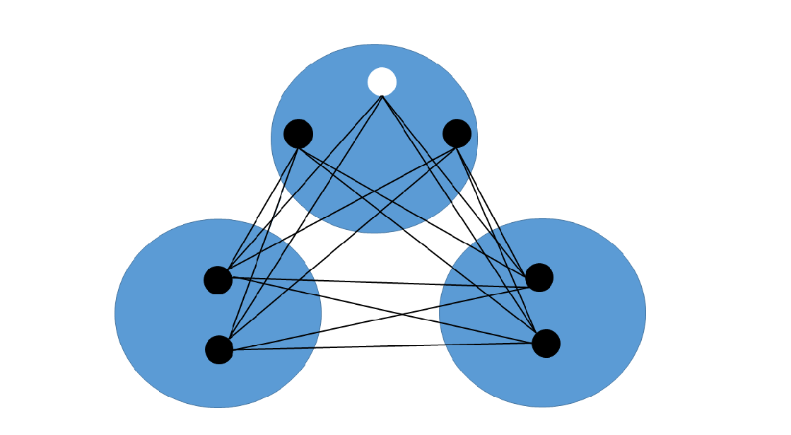
Figure 1: A UCPG graph $G(V_{0},V_{1},V_{2})$ where $m_{0}=3$ and $m_{1}=2$. The white element is the marked element $|\omega\rangle$ that resides in partition $V_{0}$.

Without loss of generality, let us assume the marked vertex $|\omega\rangle$ is in $V_{0}$ and $m_{0}\gg 1$. Define the subspace that is spanned by $|\omega\rangle,|S_{V_{0}-\omega}\rangle,|S_{{V}_{1}}\rangle,\cdots,|S_{{V}_{P}}\rangle$. With renormalization, we have

$$|S_{V_{0}-\omega}\rangle=\frac{1}{\sqrt{m_{0}-1}}\sum_{i\in V_{0},i\neq\omega}|i\rangle,\quad|S_{{V}_{i}}\rangle=\frac{1}{\sqrt{m_{i}}}\sum_{j\in S_{{V}_{i}},i\neq 0}|j\rangle$$ (5)

The adjacency matrix Hamiltonian $H_{a}$ of a given UCPG graph can thus be written in the basis states $(|\omega\rangle,|S_{V_{0}-\omega}\rangle,|S_{{V}_{1}}\rangle,\cdots,|S_{{V}_{P}}\rangle)$ and it behaves as the following:

$$H_{a}|\omega\rangle = \sum_{j=1}^{P}\sqrt{m_{j}}|S_{{V}_{j}}\rangle,\quad\quad H_{a}|S_{V_{0}-\omega}\rangle=\sum_{j=1}^{P}\sqrt{(m_{0}-1)m_{j}}|S_{{V}_{j}}\rangle$$ (6)

$$H_{a}|S_{{V}_{i},i\neq 0}\rangle = \sqrt{m_{i}}|\omega\rangle+\sqrt{(m_{0}-1)(m_{i})}|S_{V_{0}-\omega}\rangle+\sum_{j,j\neq i,j\neq 0}^{P}\sqrt{m_{i}m_{j}}|S_{{V}_{j}}\rangle.$$ (7)

By use of Lanczos algorithm and the fact that partitions not containing $|\omega\rangle$ have the same size, the reduced adjacency Hamiltonian $H_{ra}$ in the $(|\omega\rangle,|S_{V_{0}-\omega}\rangle,|S_{\bar{V}_{0}}\rangle)$ basis is

$$H_{ra}=\begin{bmatrix}0&0&\sqrt{N-m_{0}}\\ 0&0&\sqrt{(N-m_{0})(m_{0}-1)}\\ \sqrt{N-m_{0}}&\sqrt{(N-m_{0})(m_{0}-1)}&N-m_{0}-m_{1}\\ \end{bmatrix}$$ (8)

where $|S_{\bar{V}_{0}}\rangle=\frac{1}{\sqrt{N-m_{0}}}\sum_{j=1}^{P}\sqrt{m_{j}}|S_{{V}_{j}}\rangle$.

3.2 Hamiltonian Construction and Basis Change

For simplicity, let us define $\alpha=\frac{m_{0}}{N}$ and $\alpha_{1}=\frac{m_{1}}{N}$. Since $H_{ra}$ expressed in the $(|\omega\rangle,|S_{V_{0}-\omega}\rangle,|S_{\bar{V}_{0}}\rangle)$ basis captures the same dynamics as $H_{a}$, the Hamiltonian of a CTQW can be defined as [childs2004spatial]

$$H_{seek}=-\gamma H_{ra}-|\omega\rangle\langle\omega|$$ (9)

where $\gamma$ is the coupling parameter between connected vertices. By Eqn.(8, 9), we know $H_{seek}=H^{(0)}+H^{(1)}$ in the $(\omega,S_{V_{0}-\omega},S_{\bar{V}_{0}})$ basis is

$$H^{(0)}=\begin{bmatrix}-1&0&0\\ 0&0&-\gamma N\sqrt{\alpha(1-\alpha)}\\ 0&-\gamma N\sqrt{\alpha(1-\alpha)}&-\gamma N((1-\alpha)-\frac{P\alpha_{1}^{2}}{1-\alpha})\\ \end{bmatrix}$$ (10)

$$H^{(1)}=\begin{bmatrix}0&0&-\gamma\sqrt{(1-\alpha)N}\\ 0&0&0\\ -\gamma\sqrt{(1-\alpha)N}&0&0\\ \end{bmatrix}.$$ (11)

Prior to proceeding further, it is worth noticing that the format of this reduced Hamiltonian differs from the format derived in [novo2015systematic] for a complete bipartite graph. The difference is the existence of a self-loop entry for the basis vector $S_{\bar{V}_{0}}$. It later propagates in $H_{seek}$ and $H^{(0)}$. Because of this entry, in order to do systematic dimensionality reduction, it imposes a stronger constraint of equal size for partitions that do not contain the solution. We address this issue in order to generalize the result shown in [novo2015systematic] for UCPG. As verified in section LABEL:sect:Examples, we know our generalization does encompass the result from [novo2015systematic].

In the remaining of the section, we introduce Theorem 1, Lemma LABEL:lma:facts and Theorem LABEL:thm:gammavalue. The relationships among them provide the foundation for showing the optimality preserving of the underlying CTQW. The optimality preserving is explained in subsection LABEL:sect:HamilSearchG. Theorem 1 provides us the technique to construct the reduced Hamiltonian $H_{seek}$ in the eigenbasis $(|\omega\rangle,|e_{1}\rangle,|e_{2}\rangle)$ of $H^{(0)}$. Lemma LABEL:lma:facts discovers important properties of Hamiltonian $H_{seek}$ written in the eigenbasis $(|\omega\rangle,|e_{1}\rangle,|e_{2}\rangle)$ to be used in Theorem LABEL:thm:gammavalue. Theorem LABEL:thm:gammavalue shows the necessary condition for fast transport to occur in $H_{seek}$ by tuning the coupling factor $\gamma$.

Now we prove Theorem 1 to show how to express a reduced Hamiltonian $H_{seek}$ in the basis of its major matrix via perturbation theory. For simplicity, let us simply call $H_{seek}$ as $H$ in the theorem.

Theorem 1.

Given a reduced Hamiltonian $H=H^{(0)}+H^{(1)}$ in the $(|\omega\rangle,|b_{1}\rangle,|b_{2}\rangle)$ basis where

$$H^{(0)}=\begin{bmatrix}-1&0&0\\ 0&0&v_{1}\\ 0&v_{1}&v_{3}\\ \end{bmatrix},\quad H^{(1)}=\begin{bmatrix}0&0&v_{2}\\ 0&0&0\\ v_{2}&0&0\\ \end{bmatrix}$$ (12)

$v_{1}$ and $v_{2}$ are negative numbers and $v_{3}$ is a non-positive number where $v_{1}/v_{2}=\sqrt{N\alpha}\geq 1$. Let the eigenvectors basis of $H^{(0)}$ be $(|\omega\rangle,|e_{1}\rangle,|e_{2}\rangle)$. We choose $\kappa=\frac{v_{3}}{v_{1}}\geq 0$ and $\beta_{\pm}=\frac{\kappa\pm\sqrt{\kappa^{2}+4}}{2}$, then we know eigenvector $|e_{1}\rangle=\frac{(|b_{1}\rangle+\beta_{+}|b_{2}\rangle)}{\sqrt{1+\beta_{+}^{2}}}$ and eigenvector $|e_{2}\rangle=\frac{(|b_{1}\rangle+\beta_{-}|b_{2}\rangle)}{\sqrt{1+\beta_{-}^{2}}}$ where the corresponding eigenvalues are $\lambda_{\pm}=v_{1}\beta_{\pm}$. $H$ can thus be written in the $(|\omega\rangle,|e_{1}\rangle,|e_{2}\rangle)$ eigenbasis as

$$H=\begin{bmatrix}-1&v_{2}\frac{\beta_{+}}{\sqrt{\beta_{+}^{2}+1}}&v_{2}\frac{\beta_{-}}{\sqrt{\beta_{-}^{2}+1}}\\ \frac{v_{2}\sqrt{\beta_{+}^{2}+1}}{\beta_{+}-\beta_{-}}&\lambda_{+}&0\\ \frac{-v_{2}\sqrt{\beta_{-}^{2}+1}}{\beta_{+}-\beta_{-}}&0&\lambda_{-}\\ \end{bmatrix}.$$ (13)

Proof.

It is clear to see that $|e_{1}\rangle$ and $|e_{2}\rangle$ are both vectors of linear combination of $|b_{1}\rangle$ and $|b_{2}\rangle$. Without loss of generality, let $|e^{\prime}\rangle=|b_{1}\rangle+\beta|b_{2}\rangle$ be an eigenvector of $H^{(0)}$ with eigenvalue $\lambda$. After some calculation we obtain $\lambda={\beta v_{1}}$ where

$$\beta=\frac{\kappa\pm\sqrt{\kappa^{2}+4}}{2},\quad\kappa=\frac{v_{3}}{v_{1}}.$$ (14)

For simplicity, let $\beta_{+}$ be $\frac{\kappa+\sqrt{\kappa^{2}+4}}{2}$ and $\beta_{-}$ be $\frac{\kappa-\sqrt{\kappa^{2}+4}}{2}$. By renormalizing the eigenvectors $|e^{\prime}_{1}\rangle=|b_{1}\rangle+\beta_{+}|b_{2}\rangle$, $|e^{\prime}_{2}\rangle=|b_{1}\rangle+\beta_{-}|b_{2}\rangle$, we have

$${}|e_{1}\rangle=\frac{|e^{\prime}_{1}\rangle}{\sqrt{\beta_{+}^{2}+1}},\quad|e_{2}\rangle=\frac{|e^{\prime}_{2}\rangle}{\sqrt{\beta_{-}^{2}+1}}$$ (15)

such that

$$H^{(0)}|e_{1}\rangle=\lambda_{+}|e_{1}\rangle,\quad H^{(0)}|e_{2}\rangle=\lambda_{-}|e_{2}\rangle$$ (16)

where

$$\lambda_{\pm}=\beta_{\pm}v_{1}.$$ (17)

In the $(|\omega\rangle,|b_{1}\rangle,|b_{2}\rangle)$ eigenbasis, from Eqn.(12) we know $H^{(1)}|b_{1}\rangle=0$, $H^{(1)}|\omega\rangle=v_{2}|b_{2}\rangle$ and $H^{(1)}|b_{2}\rangle=v_{2}|\omega\rangle$. To express $H^{(1)}$ in the $(|\omega\rangle,|e_{1}\rangle,|e_{2}\rangle)$ eigenbasis, by simple basis change, we obtain

$$H^{(1)}|e_{1}\rangle=v_{2}(\beta_{+}/(\sqrt{\beta_{+}^{2}+1}))|\omega\rangle,\quad H^{(1)}|e_{2}\rangle=v_{2}(\beta_{-}/(\sqrt{\beta_{-}^{2}+1}))|\omega\rangle$$ (18)

$$H^{(1)}|\omega\rangle=v_{2}|b_{2}\rangle=\frac{v_{2}\sqrt{\beta_{+}^{2}+1}}{\beta_{+}-\beta_{-}}|e_{1}\rangle+\frac{-v_{2}\sqrt{\beta_{-}^{2}+1}}{\beta_{+}-\beta_{-}}|e_{2}\rangle.$$ (19)

Hence, the Hamiltonian $H$ can be expressed as shown in Eqn. (13). ∎