The stepwise path integral of the relativistic point particle

Abstract

In this paper we present a stepwise construction of the path integral over relativistic orbits in Euclidean spacetime. It is shown that the apparent problems of this path integral, like the breakdown of the naive Chapman-Kolmogorov relation, can be solved by a careful analysis of the overcounting associated with local and global symmetries. Based on this, the direct calculation of the quantum propagator of the relativistic point particle in the path integral formulation results from a simple and purely geometric construction.

1 Introduction

Local Lagrangian symmetries and relativity are essential in modern quantum physics. However, the simplest unification attempt fails dramatically: Lagrangian path integrals of relativistic point particles are considered intractable. The novelty of this article is that by considering a previously unnoticed symmetry, those problems are overcome and an exact calculation of the full propagator of the relativistic point particle is achieved.

If one remembers that the relativistic point particle is the simplest system with general covariance, it becomes clear that its understanding will be crucial for the consistent formulation of more complex theories with the same (extended) symmetry such as quantum gravity or string theory.

1.1 The problem

Since the first applications in non-relativistic quantum mechanics Feynman:1950ir , the path integral formulation of quantum theories has developed in huge steps towards a quantum field theory of fundamental interactions. A common consequence of advancing in huge steps is that one leaves obstacles and possible subtleties unexplored on the way. This happened with the Path Integral (PI) formulation of the relativistic point particle. It is the purpose of this paper to close that gap and to resolve some misconceptions and problems that persisted until today in the context of this fundamental topic.

Even though, the PI of the relativistic point particle is the logical continuation of the non-relativistic PI it has been largely omitted on the way to quantum field theory. One reason is that attempts to realize the PI of the relativistic point particle has presented large complications Teitelboim:1982 ; Henneaux:1982ma ; Redmount:1990mi ; Fradkin:1991ci ; Padmanabhan:1994 . Among them, one can distinguish between those that seem to be of technical nature and those that seem to be of conceptual nature.

• Technical complications:
  At the first sight a technical issue arises from the appearance of non-Gaussian integrals. This issue can be avoided by the use of auxiliary field variables in the Hamiltonian action, which allow to relate (at least at the classical level) the original action to a quadratic action Brink:1976 ; Brink:1977 ; Fradkin:1991ci , which is sometimes called einbein formalism. Those methods, allow to obtain the expected Klein Gordon propagator from the PI of the relativistic point particle in $D$ dimensions

  $$K\sim\frac{1}{(k^{2}+M^{2})}.$$ (1)

  As shown in the Appendix A, a direct calculation of the PI with the Lagrangian action in $D$ dimensions and without auxiliary fields is actually possible. The problem is however, that it leads to a propagator

  $$K^{(n)}\sim\frac{1}{(k^{2}+M^{2})^{n(D+1)/2}}.$$ (2)

  Here, $n$ is the number of intermediate slices. Apparently (2) does not have the expected form of (1). This difference was the first motivation for this study on the direct PI of the relativistic point particle.

• Conceptual complications:
  Leaving the technical issues aside, there is a much more disturbing fact that complicates the understanding of the PI of the relativistic point particle: The Chapman-Kolmogorov (CK) equation for Markovian processes is not satisfied. This means that the standard notion of probability is not preserved in the process of free relativistic propagation.

  As an example, let’s show this for the propagator (1) in position space

  $$K(0,\vec{x})=\mathcal{N}\int d^{D}k\frac{\exp(i\vec{k}\cdot\vec{x})\sqrt{2}M}{k^{2}+M^{2}},$$ (3)

  where $\mathcal{N}$ is a normalization constant. The usual CK condition sates that: “Propagating from $0$ to $\vec{x}_{1}$ and then from $\vec{x}_{1}$ to $\vec{x}_{2}$ and finally integrating over all $\vec{x}_{1}$, must be equivalent to propagating from $0$ to $\vec{x}_{2}$”. Applying this definition to the propagator (3) gives

  $$Kol(0,\vec{x}_{2}) = \int d^{D}x_{1}K(0,\vec{x}_{1})K(\vec{x}_{1},\vec{x}_{2})$$ (4)

  $$= \mathcal{N}^{2}\int d^{D}k\frac{\exp(i\vec{k}\cdot\vec{x}_{2})2M^{2}}{(k^{2}+M^{2})^{2}}.$$

  This is of course not the form of the original propagator (3), which is the well known and un-understood problem of the path integral of the relativistic point particle.

  In the literature there exist different stances on this embarrassing problem. Mostly, it is just taken as hint that at relativistic velocities the assumption of a single particle theory breaks down. It is argued that the energy available at such velocities would allow for interactions that again allow for the production of multi particle state  Kleinert:book . This argument is however not very convincing since one was dealing with a free theory without interactions at the first place. Another stance is to try to fix this problem by the redefinition of the probability measure Jizba:2008 ; Jizba:2010pi .

In this paper we propose an elegant solution to those two fundamental problems. In Koch:2017bvv it has been shown that for the case of the relativistic point particle action it is important to consider a particular local symmetry of the corresponding action. The preceding paper Koch:2017bvv further shows how formal symmetry considerations in Minkowski spacetime in combination with the Fadeev-Popov procedure Faddeev:1967fc allow to perform the full functional path integral of the relativistic point particle. The idea of this paper is to abstain from abstract technical formulations and to show instead that the problem can be perfectly understood and solved by very basic geometric considerations. Further, several additional explicit calculations and complementary examples are shown below.

The paper is organized as follows: The introduction is completed by making notion of the symmetries of the relativistic point particle and by a definition of the PI measure taking into account those symmetries. In section II several Euclidean PIs with one intermediate step are calculated in arbitrary dimensions and in section III it is proven that those one-step propagators are already the full propagators for the given theory. Section IV contains a discussion on the CK relation and the conclusion. Throughout the paper all formulas and discussions will be given in the imaginary time formalism corresponding to the Euclidean metric.

1.2 The relativistic point particle

The action for a relativistic point particle in $D$ dimensions is

$$S=\int_{\lambda_{i}}^{\lambda_{f}}d\lambda\cdot m\sqrt{\left(\frac{d\vec{x}}{d\lambda}\right)^{2}},$$ (5)

with $\vec{x}(\lambda_{i})=\vec{x}_{i}$ and $\vec{x}(\lambda_{f})=\vec{x}_{f}$. This is simply the mass times the geometric length of a given path $\mathcal{P}$. It is interesting to note that this action in Minkowski space-time can not be equivalent to the action in the einbein formalism Brink:1976 ; Brink:1977 ; Fradkin:1991ci , for space-like and timelike paths. This can be seen from the fact that the integration over timelike and space-like paths with (5) would involve both complex and real values for the action. Thus, the Euclidean path integral over (5) means probably a restriction on the type of paths that is allowed in the non-Euclidean version of the path integral. A detailed analysis of the corresponding integral in Minkowski space-time will be given in Koch:2018 .

This action and its corresponding Lagrangian are equipped with several symmetries which will be important for the formulation of a consistent path integral.

• Global Poincaré invariance: This can be seen from the fact that the action is invariant under global rotations and shifts of the coordinate system in $D$ dimensions.

• Local Lorentz invariance: This means that the Lagrangian is invariant under local rotations in $D$ dimensions of the vector $(d\vec{x})/(d\lambda)$ at any point along the trajectory. A formal argument on why this symmetry, which is not a classical gauge symmetry, is actually important in this given context was given in Koch:2017bvv .

• Weyl invariance: This means that the Lagrangian does not depend on the way that $\lambda$ parametrizes a path $\mathcal{P}$. The change to any other function $\tilde{\lambda}(\lambda)$ would leave the Lagrangian invariant.

In the following the symmetry (a) will be used to choose the coordinate system such that $\vec{x}_{i}=0$ and that $\vec{x}_{f}$ is different from zero in only one component. The symmetries (b) and (c) are symmetries which have to be treated with care when it comes to realizing an integral over different paths, since two seemingly different paths could be actually physically equivalent. The over-counting of physically equivalent paths would result in a wrong weight of some paths with respect to others.

1.3 General considerations on the explicit form of the PI measure

When one formally writes the functional integral ${\mathcal{D}}x(\lambda)$ one has to give a clear definition of this measure. The common definition of the PI measure is

$$K(x_{i},x_{f}) \equiv \int_{\vec{x}(t_{i})=\vec{x}_{i}}^{\vec{x}(t_{f})=\vec{x}_{f}}{\mathcal{D}}x(\lambda)\exp\left[-\int dt{\mathcal{L}}\right]$$

$$= \lim_{n\rightarrow\infty}{\mathcal{N}}_{D,n}(t)\prod_{j=1}^{n}\int dx_{j}^{D}\exp\left[-\sum_{j}\Delta t{\mathcal{L}}_{j}\right]$$

$$= \lim_{n\rightarrow\infty}K^{(n)}(x_{i},x_{f}),$$

where the normalization ${\mathcal{N}}_{D,n}(t)$ is a function of the external time $t$, the number of time slicings $n$ used, and of the dimensions $D$. Usually this normalization is fixed from imposing the Kolmogorov relations. However, there are several issues that arise when one tries to apply this naive measure (1.3) to the relativistic point particle which are all related to an overcounting of certain paths:

It is easy to see that in the definition (1.3) one is not just counting any possible path between $\vec{x}_{i}$ and $\vec{x}_{f}$. One actually counts paths which have straight sections multiple times. Let’s exemplify this for the case of two slicings $n=2$. All configurations where the position $\vec{x}_{1}$ is on the classical path between $\vec{x}_{i}\rightarrow\vec{x}_{2}$ correspond actually to the same path $\vec{x}_{i}\rightarrow\vec{x}_{2}\rightarrow\vec{x}_{f}$ as it is shown in figure 1.

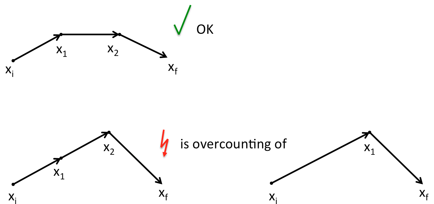
Figure 1: Exemplification of possible overcounting of one path with two intermediate steps, which is already counted in the PI with one intermediate step.

Strictly speaking they should only be counted once but according to (1.3) this path would be counted multiple times. Usually, this type of overcounting is completely irrelevant, since the number of paths that are not overcounted grows much faster with $n$ and $D$ than the number of paths where this overcounting occurs. In simple words, it is very unlikely that $\vec{x}_{1}$ happens to be on the classical path between $\vec{x}_{i}\rightarrow\vec{x}_{2}$. However, in problems with local symmetries this might not necessarily be the case. In order to avoid overcounting of identical paths right from the start, one can improve (1.3) by stating for $K=K(x_{i},x_{f})$

$$K \equiv \lim_{n\rightarrow\infty}\sum_{j=1}^{n}K^{(j)}(x_{i},x_{f})$$ (8)

$$\equiv \left.\lim_{n\rightarrow\infty}\sum_{j=1}^{n}{\mathcal{N}}_{D,j}(t)\prod_{l=1}^{j}\int dx_{l}^{D}\right|_{NOC}\exp\left[-\sum_{j}\Delta t{\mathcal{L}}_{j}\right]$$

$$= {\mathcal{N}}_{D,1}(t)\left.\int dx^{D}_{1}\right|_{NOC}\exp\left[-t/2({\mathcal{L}}_{i,1}+{\mathcal{L}}_{1,f})\right]+$$

$${\mathcal{N}}_{D,2}(t)\left.\int dx^{D}_{1}\int dx^{D}_{2}\right|_{NOC}\exp\left[-t/3({\mathcal{L}}_{i,1}+\dots)\right]$$

$$+\dots,$$

where $|_{NOC}$ stands “integrate but without overcountig” in the sense described before. For example, when performing the two slicing integral one has to avoid overcounting of configurations which are equivalent to one slicing paths and when doing higher number of slicings ($j=n$) one has to avoid all the configurations which are actually already counted in ($j<n$) paths. Even thought this definition is morally superior to (1.3), it is in most cases highly impractical since one has to take into account numerous conditions when actually performing the integrals. Fortunately, in most cases, the term with the highest number of integrals $j=n$ represents a $D+n$ dimensional volume which dominates the sub-leading contribution which is a $D+n-1$ dimensional volume and the definition (8) is equivalent to (1.3).

Even though, the overcounting issue seems to be settled by the definition (8), one has to be careful, since imposing a $|_{NOC}$ condition means in most practical cases a fixing of the symmetry. Different fixings can correspond to different restrictions of the measure, which would generate unphysical anomalies Fujikawa:1979ay . However, we expect that the symmetries of the action are also symmetries of the measure. This can be solved by redefining the measure with a multiplicative factor $\Delta_{i}$ such that it is invariant under different configurations within the symmetry

$$K \equiv \left.\lim_{n\rightarrow\infty}\sum_{j=1}^{n}{\mathcal{N}}_{D,j}(t)\prod_{l=1}^{j}\int dx_{l}^{D}\right|_{NOC}\Delta_{l}e^{\left[-\sum_{r}t_{r+1,r}{\mathcal{L}}_{r+1,r}\right]}$$ (9)

$$= {\mathcal{N}}_{D,1}(t)\left.\int dx^{D}_{1}\right|_{NOC}\Delta_{1}\exp\left[-t_{1,i}{\mathcal{L}}_{i,1}-t_{1,f}{\mathcal{L}}_{1,f})\right]$$

$$+{\mathcal{N}}_{D,2}(t)\left.\int dx^{D}_{1}\int dx^{D}_{2}\right|_{NOC}\Delta_{2}\exp\left[\dots\right]+\dots.$$

The external normalization factors ${\mathcal{N}}_{D,j}(t)$ are fixed by a dimensional argument.

Relation (9) is the definition of the measure ${\mathcal{D}}x$, that will now be used for the PI of the relativistic point particle.

2 Euclidean path integrals with one intermediate step

In this section we will discuss how the considerations on the measure, overcounting, and symmetries, are applied to the one-slicing propagator $K^{(1)}$. This will be explicitly done in one and two dimensions, before it is generalized to $D$ dimensions. Before actually turning to the relativistic point particle it is instructive to discuss (9), in particular the meaning of the restriction $|_{NOC}$, for the case of non-relativistic quantum mechanics.

2.1 The non-relativistic path integral in two dimensions

Some of the redundancies that will be important for the relativistic case are already present in the path integral of the non-relativistic point particle. It is therefore instructive to discuss this case first and to show that in the non-relativistic case the over-counting over equivalent paths does not do any harm since it can be absorbed into a constant normalization factor. For the classical Lagrangian $\vec{v}^{2}/(2M)$ one can construct the propagator with one intermediate step by composing two propagations with time lapse $\Delta t/2$ each $K^{(1)}(\vec{x}_{i},\vec{x}_{f})=K^{(1)}$ reads

$$K^{(1)}=\int d^{D}x_{1}\cdot{\mathcal{N}}_{1}\exp\left[-\frac{M}{2}\left(\frac{(\vec{x}_{1}-\vec{x}_{i})^{2}}{\Delta t/2}+\frac{(\vec{x}_{f}-\vec{x}_{1})^{2}}{\Delta t/2}\right)\right].$$ (10)

There are two Lagrangians and one action in this problem which are

$${\mathcal{L}}_{i1} = 2M\left(\frac{(\vec{x}_{1}-\vec{x}_{i})^{2}}{\Delta t^{2}}\right),$$

$${\mathcal{L}}_{1f} = 2M\left(\frac{(\vec{x}_{f}-\vec{x}_{1})^{2}}{\Delta t^{2}}\right),\;{\mbox{and}}$$

$$S = \Delta t\left({\mathcal{L}}_{i1}+{\mathcal{L}}_{1f}\right).$$ (11)

Now one wants to see whether there are local transformations which allow to apply a continuous change of $\vec{x}_{1}$ while leaving ${\mathcal{L}}_{i1}$ and ${\mathcal{L}}_{1f}$ invariant. For $D=2$ one finds that those two conditions completely fix the values of $\vec{x}_{1}$ as long as $\vec{x}_{i}\neq\vec{x}_{f}$. Thus, there is no overcounting in the propagator in two dimensions as long as $\vec{x}_{i}\neq\vec{x}_{f}$. At first sight it seems that with identical initial and final positions, there is an overcounting, even for $D=2$. But this is actually not the case, since seemingly equivalent paths become distinguishable, when seen from a different Galilelian reference system. Thus, for non-relativistic paths with two spatial dimensions, there is no overcounting. However, when $D\geq 3$, there is an additional freedom in the orientation of the vector $\vec{x}_{i}+\vec{x}_{1}$ with respect to $\vec{x}_{i}$. This situation is shown in figure 2.

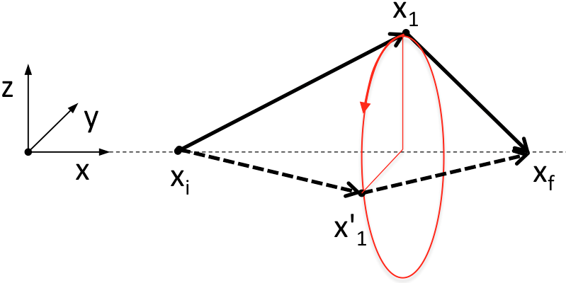
Figure 2: Non-relativistic PI in three dimensions with equivalent intermediate points $\vec{x}_{1}$.

This additional freedom corresponds to paths which are all redundant since they do not change any of the terms in (11). Thus, due to the $|_{NOC}$ condition in (9), those paths should not be included when integrating. The question that arises is, does this $|_{NOC}$ condition affect the usual propagator in non-relativistic quantum mechanics?

In order to see this redundant part of the integral more clearly one can perform a series of coordinate transformations. First one shifts the integration variables $\vec{x}^{\prime}=\vec{x}-(\vec{x}_{f}-\vec{x}_{i})/2$, then one goes to radial coordinates in three dimensions $\{x^{\prime},y^{\prime},z^{\prime}\}\rightarrow\{r,\theta,\alpha\}$ with the Jacobian $dx^{\prime}dy^{\prime}dz^{\prime}\rightarrow dr\sin(\theta)d\theta d\alpha$, and finally one changes the radial integration for an integration over the action $dr\rightarrow dS(dr/dS)$ according to (11). Integrating over $\theta$ gives

$$K^{(1)}(\vec{x}_{i},\vec{x}_{f}) = \left(\int_{0}^{2\pi}d\alpha\right)\frac{(\Delta t)^{3/2}}{(2M)^{3/2}}$$

$$\cdot\int_{S_{c}}^{\infty}dS\exp[-S]\sqrt{S-S_{c}}\cdot{\mathcal{N}}_{1}.$$

Thus,

$$K^{(1)}(\vec{x}_{i},\vec{x}_{f})=\left(\int_{0}^{2\pi}d\alpha\right)\frac{(\Delta t)^{3/2}}{(2M)^{3/2}}\frac{\sqrt{\pi}}{2}\exp[-S_{c}]{\mathcal{N}}_{1},$$ (13)

where $\mathcal{N}_{1}$ is assumed to be position independent and where $S_{c}=\frac{M}{2}\frac{(\vec{x}_{f}-\vec{x}_{i})^{2}}{\Delta t}$. One observes from (13) that the volume corresponding to the overcounting of local rotations $d\alpha$ factors out nicely. Note that this coordinate transformation corresponds to the one-slicing version of the Fadeev-Popov procedure. Finally, one sees from this relation that one can choose a simple normalization

$${\mathcal{N}}_{1}=\frac{2(2M)^{3/2}}{\left(\int_{0}^{2\pi}d\alpha\right)\sqrt{\pi}\Delta t^{3/2}},$$ (14)

such that the classical propagator $K^{(0)}\sim\exp(-S_{c})$ fulfills the Kolmogorov relation

$$K^{(0)}(\vec{x}_{i},\vec{x}_{f})=\int dx_{1}dy_{1}dz_{1}K^{(0)}(\vec{x}_{i},\vec{x}_{1})K^{(0)}(\vec{x}_{1},\vec{x}_{f}).$$ (15)

The important point of this discussion is that instead of integrating over the equivalent configurations one could actually fix the angle $\alpha$ to some value which corresponds to dividing (13) by a factor of $2\pi$. When one does this fixing, one also has to exclude those redundant configurations in the non-relativistic Kolmogorov relation (15).

However, since all this symmetry fixing at the end of the day results in a simple rescaling of the normalization (14) by a factor of $2\pi$, one sees that considering the symmetry (b) actually leaves all results of non-relativistic quantum mechanics unchanged. The situation is different for the relativistic path integral, as shown in the following subsections.

2.2 The relativistic path integral in one dimension

Let’s start the discussion of the relativistic PI with the most simple case, paths in one dimension. Already this case shows some non-trivial features since even though there is no global or local Lorentz symmetry, the Weyl symmetry (c) is already present in this case. As usual, one can fix this symmetry by choosing a unit length evolution parameter such that for each path

$$\left(\frac{d\vec{x}}{d\lambda}\right)^{2}=1,$$ (16)

for which the Lagrangian reads

$${\mathcal{L}}=M.$$ (17)

The fundamental building block of the path integral is the exponential of the classical action times some normalization constant which we will choose equal to $M$ for the one dimensional case

$$K^{(0)}(x_{i},x_{f})=M\cdot\exp(-M|x_{f}-x_{i}|).$$ (18)

The next step towards constructing the relativistic path integral in one dimension consists in introducing one intermediate slice $x_{1}$. According to (9), the one slicing propagator $K^{(1)}(x_{i},x_{f})=K^{(1)}$ would then be

$$K^{(1)} = {\mathcal{N}}_{1,1}(t_{i,f})\int_{-\infty}^{+\infty}dx_{1}|_{NOC}\Delta_{1}\cdot$$ (19)

$$K^{(0)}(x_{i},x_{1})\cdot K^{(0)}(x_{1},x_{f}).$$

The normalization and the anomaly cancelation in one dimension is trivial ${\mathcal{N}}_{1,1}(t)=1=\Delta_{1}$. Before integrating, one has still to take into account the redundancy explained in figure 1. Whenever $x_{1}$ is between $x_{i}$ and $x_{f}$, the two-step propagation $x_{i}\rightarrow x_{1}\rightarrow x_{f}$ is physically exactly the same path as the direct connection $x_{i}\rightarrow x_{f}$ and should not be counted over and over again. Thus, according to (9) the right one-step propagator in one dimension $K^{(1)}(x_{i},x_{f})|_{NOC}=\tilde{K}^{(1)}$ is

$$\tilde{K}^{(1)} = \int_{-\infty}^{x_{i}}dx_{1}K^{(0)}(x_{i},x_{1})\cdot K^{(0)}(x_{1},x_{f})$$

$$+\int_{x_{f}}^{+\infty}dx_{1}K^{(0)}(x_{i},x_{1})\cdot K^{(0)}(x_{1},x_{f}),$$

where we assumed $x_{f}>x_{i}$. A trivial integration gives

$$K^{(1)}(x_{i},x_{f})|_{NOC}=M\cdot\exp(-M|x_{f}-x_{i}|)=K^{(0)}(x_{i},x_{f}),$$ (21)

which means that for one dimension the initial expression (18) is equal to the one slicing propagator (21). This has important consequences for the generalization to $n$ intermediate steps, as it will be discussed in a later section.

Remember that due to the fact that the one dimensional case does not have the local symmetry b) it was possible to waive all length dependent normalization factors defined in (9) and choose ${\mathcal{N}}({t,1,1})=1=\Delta_{1}$. For the two dimensional case, the symmetry b) is present and thus one has to consider those non-trivial contributions.

2.3 The relativistic path integral in two dimensions

It is instructive to continue the discussion of the problem in two dimensions with one intermediate step. According to (9), the right one-slice propagator $K^{(1)}(\vec{x}_{i},\vec{x}_{f})=K^{(1)}$ is

$$K^{(1)} = {\mathcal{N}}_{D,1}(t_{i,f})\int d^{D}x_{1}|_{NOC}\Delta_{1}\cdot$$

$$\exp{[-S_{0}(\vec{x}_{i},\vec{x}_{1})]}\cdot\exp{[-S_{0}(\vec{x}_{1},\vec{x}_{f}))]}.$$

In two Euclidean dimensions ($\vec{x}=(x(\lambda),y(\lambda))$), the relativistic path integral (2.3) reads

$$K^{(1)} = {\mathcal{N}}_{2,1}(t_{i,f})\int d^{2}x_{1}|_{NOC}\Delta_{1}\cdot$$

$$\exp{\left[-M|\vec{x}_{1}-\vec{x}_{i}|-M|\vec{x}_{f}-\vec{x}_{1}|\right]}.$$

For simplicity let’s choose the initial position as origin of the Cartesian coordinate system $\vec{x}_{i}=0$. As part of this integral one can consider paths that all contribute with the same action to this path integral. One finds that the surface of points with equal action is shown by the ellipse in figure 3. This curve is generated by all different paths ($\vec{x}_{i}\rightarrow\vec{x}_{1}\rightarrow\vec{x}_{f}$) with the same total length.

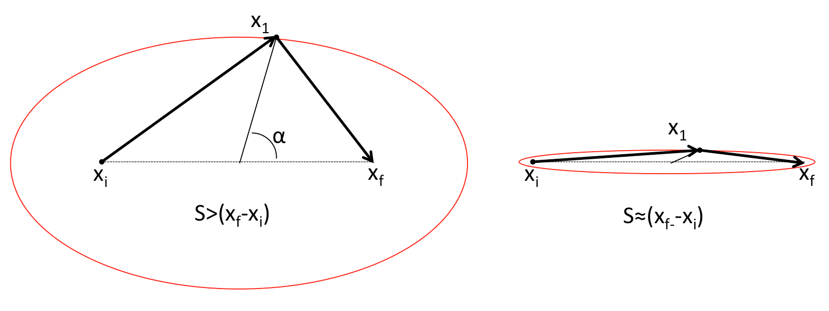
Figure 3: Left: Relativistic PI in two dimensions for paths with same action $S$, where the red curve represents all equivalent points $x_{1}$ for a given action value $S>S_{cl}$. Right: It is interesting to note that in the classical limit, when $S\rightarrow S_{cl}$, the elliptic contour of equivalent points $x_{1}$ collapses to the classical path. This means that the two local symmetries (b) and (c) are indistinguishable at the classical level.

However, the important feature of the relativistic case is that the Lagrangian (17) is the same for every single point along any of those paths with $S=const.$ and $\vec{x}_{i},\,\vec{x}_{f}$ fixed. This is a reflection of the fact that local Lorentz symmetry (b) has not been fixed. Thus, if one naively counts all the points on the relativistic elliptic contour in figure 3, one is actually counting paths which are connected by a symmetry transformation. Instead, one should count only one point out of the elliptic contour by properly fixing the freedom introduced by the symmetry (b).

In order to cast the integral (2.3) in the equal-action form

$$K^{(1)}(0,\vec{x}_{f}) = \int_{S_{0}}^{\infty}dS\exp(-S)\cdot\Omega_{R,2}^{(1)}(S;0,\vec{x}_{f}),$$ (24)

one can transform the Cartesian coordinates $x_{1},y_{1}$ into slightly modified elliptical coordinates $\chi_{i}=(S,\,\alpha)$, with

$$x_{1} = \frac{S}{2M}\cos(\alpha),$$ (25)

$$y_{1} = \frac{x_{f}}{2}\sqrt{\left(\frac{S}{x_{f}M}\right)^{2}-1}\cdot\sin(\alpha).$$ (26)

Here, we have chosen the middle of the classical path $0\rightarrow\vec{x}_{f}$ as the origin of the elliptical coordinate system and $\alpha$ as the angle between the $x$ axes and the vector $\vec{x}_{1}-(\vec{x}_{f}-\vec{x}_{i})$, as shown in figure 3. Further, for the Cartesian choice $\vec{x}_{i}=0$, $x_{f}=|\vec{x}_{f}-0|$ stands for the length of the minimal classical path, while $S$ stands for the length of the quantum path $0\rightarrow\vec{x}_{1}\rightarrow\vec{x}_{f}$. The Jacobian of the coordinate transformation is

$$\det\left(\frac{x_{i}}{\chi_{j}}\right)=\frac{2\left(S/M\right)^{2}-x_{f}^{2}(1+\cos(2\alpha))}{8\sqrt{\left(S\right)^{2}-(x_{f}M)^{2}}}.$$ (27)

Thus the one-step propagator $K^{(1)}(0,\vec{x}_{f})=K^{(1)}$ is

$$K^{(1)} = {\mathcal{N}}_{2,1}(t_{i,f})\int_{x_{f}M}^{\infty}dS\int_{0}^{2\pi}d\alpha\cdot$$

$$\Delta_{1}\frac{2\left(S/M\right)^{2}-x_{f}^{2}(1+\cos(2\alpha))}{8\sqrt{(S)^{2}-(x_{f}M)^{2}}}\exp{[-S]}.$$

One notes that the angular integral, which represents the redundancy, does not simply factorize like in the non-relativistic case. This anomalous angular dependence in the numerator of (27) comes due to a naively defined measure $dx_{1}dy_{1}$ and has to be canceled by a proper definition of the multiplicative factor

$$\Delta_{1}^{-1}\equiv|\vec{x}_{1}-0|\cdot|\vec{x}_{f}-\vec{x}_{1}|=\frac{1}{8}\left(2\left(S/M\right)^{2}-x_{f}^{2}(1+\cos(2\alpha))\right)$$ (29)

which is the simplest non-fractional term containing $\alpha$. A dimensional analysis shows that the measure ${\mathcal{N}}_{2,1}(t_{i,f})={\mathcal{N}}_{2,1}$ in two dimensions is actually independent of $x_{f}\equiv|\vec{x}_{f}-0|$. With this, one finds

$$K^{(1)}(0,\vec{x}_{f}) = {\mathcal{N}}_{2,1}\left(\int_{0}^{2\pi}d\alpha\right)$$

$$\cdot\int_{x_{f}M}^{\infty}dS\frac{1}{\sqrt{(S)^{2}-(x_{f}M)^{2}}}\exp{[-S]}$$

$$= {\mathcal{N}}\cdot(2\pi)K_{0}(x_{f}M).$$ (31)

Please note that the redundant volume $\left(\int_{0}^{2\pi}d\alpha\right)$ can now either be eliminated by fixing the angle $\alpha$ or by integrating over the angle and absorbing the factor in the normalization of the propagator. A two dimensional Fourier transformation of (31) returns again the expected propagator of the free scalar field in Fourier space.

By comparing the one slicing propagator $K^{(1)}(x_{f})=(2\pi)K_{0}(x_{f}M)$ with the zero slicing propagator $K^{(0)}(x_{f})\sim\exp(-M|x_{f}|)$, one notes that in contrast to the one dimensional case, the Kolmogorov relation is not fulfilled when going from zero to one slicing. This makes it necessary to study a higher number of intermediate steps, which will be done after discussing the one-step case in $D$ dimensions.

2.4 The relativistic path integral in $D$ dimensions

It is straight forward to repeat the discussion of the two dimensional case for the path integral of the relativistic point particle in higher dimensions. When changing to the modified elliptical coordinates in $D$ dimensions $\chi_{i}=(S,\alpha_{1},...,\alpha_{D-1})$ one notes that for one slicing the Jacobian of the transformation takes the form

$$\det\left(\frac{x_{i}}{\chi_{j}}\right) = \left[2\left(S/M\right)^{2}-x_{f}^{2}(1+\cos(2\alpha_{1}))\right]g(\alpha_{1})$$

$$\cdot\left(S^{2}-(x_{f}M)^{2}\right)^{(D-3)/2}\cdot f(\alpha_{2},\dots\alpha_{D-1}).$$

This determinant can be written as a product of three functions, one with the angle $\alpha_{1}$, one with the angles $\alpha_{i}|_{i>1}$, and of one function without angles. Here, $g(\alpha_{1})$ and $f(\alpha_{2},\dots\alpha_{N-1})$ are the typical angular dependencies in $D$-dimensional spherical coordinates. Just like in the two dimensional case, the anomalous non-factorization of the angle $\alpha_{1}$, can be corrected by an appropriate choice of $\Delta_{1}$. An anomaly free symmetry fixing choice is again assured for the definition (29), independent of the dimension $D$. The remaining angular functions $g(\alpha_{1})\cdot f(\alpha_{2},\dots\alpha_{D-1})$ do not mix with $S$ and give simply a solid angle. Further, in order to compensate the change in dimensionality induced by each additional spatial integral one has to choose the normalization with an inverse dimensional factor of $(|\vec{x}_{f}-0|)$

$${\mathcal{N}}_{D,1}(|\vec{x}_{f}-0|)\equiv{\mathcal{N}}\cdot|\vec{x}_{f}-0|^{2-D}.$$ (33)

Note that the $x_{f}$ dependence of the normalization (33) can also be obtained from imposing a matching to the non-relativistic limit of the resulting propagator. With this normalization and after integrating the factorized solid angle, the propagator reads

$$K^{(1)} = \frac{{\mathcal{N}}}{|x_{f}|^{D-2}}\int_{x_{f}M}^{\infty}dS\exp[-S]\left(S^{2}-(x_{f}M)^{2}\right)^{(D-3)/2}.$$

By integrating over $S$ one gets the one-slicing propagator in $D$ dimensions

$$K^{(1)}(x_{f}) = {\mathcal{N}}^{\prime\prime}\left(\frac{1}{x_{f}M}\right)^{D/2-1}K_{D/2-1}(M|x_{f}|),$$ (35)

where $K_{D/2-1}$ is the modified Bessel function.

3 Euclidean path integrals with $n$ intermediate steps

Up to now we have calculated the relativistic propagator with one intermediate step $K^{(1)}_{D}$. However, according to (9) one still has to calculate infinitely many propagators with $n$ intermediate steps $K^{(n)}_{D}$ and than one has to sum them all up, taking again into account that no overcounting occurs. This sounds like a lot of work, unless one has some convenient relation (or theorem) that allows to deduce all $K^{(n)}_{D}$ and their sum just from the knowledge of $K^{(1)}_{D}$. In non-relativistic quantum mechanics, this powerful tool of simplification is given in terms of the Kolmogorov relation (15). It will now be shown, that there exists a generalization of this relation for the relativistic PI in one dimension and that for the relativistic PI in higher dimensions there exists a “nothing new theorem” which also allows to deduce $K^{(n)}_{D}$ from the knowledge of $K^{(1)}_{D}$.

3.1 One dimensional case

By taking into account the “no overcounting” condition it was previously shown that, the one-slicing propagator (21) has actually the same functional form as the fundamental infinitesimal propagator (18). Thus, by iterating this process one obtains that the $n$ step propagator $K^{(n)}(x_{i},x_{f})$ is also equal to (18) and that this propagator does fulfill the CK relation, as long as one avoids overcounting in the summation over intermediate steps $x_{1}$. Thus, summing all $K^{(n)}$ still gives

$$K_{1}(x_{f}-x_{i})\sim K_{1}^{(n)}(x_{f}-x_{i})=K_{1}^{(0)}(x_{f}-x_{i}),$$ (36)

up to a normalization constant.

It is instructive to study the one-dimensional propagator in its Fourier representation. In order to get a relation in Fourier space one can operate on both sides of (2.2) with $\int_{-\infty}^{\infty}dx_{f}\exp(+ikx_{f})$ which gives after a shift of integration variables $\tilde{x}_{f}=x_{f}-x_{1}$ on the right hand side

$$\frac{2M}{k^{2}+M^{2}}=M\frac{2M}{k^{2}+M^{2}}\cdot\frac{2M}{k^{2}+M^{2}}-2M\frac{M^{2}-k^{2}}{(k^{2}+M^{2})^{2}}.$$ (37)

This is the relativistic CK relation in Fourier space in one dimension. The unusual but essential piece is the subtraction of the $2M\frac{M^{2}-k^{2}}{(k^{2}+M^{2})^{2}}$ term which comes from the missing piece ($M\int_{0}^{x_{f}}dx_{1}\exp(-|x_{f}|)=M|x_{f}|\exp(-|x_{f}|)$ ) on the right hand side in (2.2). The physical meaning of this subtraction is that in a naive $\int_{-\infty}^{\infty}dx_{1}$ integration, the part from 0 to $x_{f}$ corresponds to over-counting of physically equivalent paths. Thus, the right hand side of (37) means that one can indeed combine two propagators $\sim 1/(k^{2}+M^{2})$ such that they give again the same form of a propagator $\sim 1/(k^{2}+M^{2})$, if one correctly subracts the overcounting part $\sim(M^{2}-k^{2})/(k^{2}+M^{2})^{2}$.

3.2 Two dimensional case

The anomaly free relativistic propagator in two dimensions with two intermediate steps without overcounting is according to the definition (9) given by

$$K^{(2)}(\vec{x}_{i},\vec{x}_{f})|_{NOC}={\mathcal{N}}\int d^{2}x_{1}d^{2}x_{2}|_{NOC}\cdot\Delta_{2}$$

$$\cdot\exp{\left[-M(|\vec{x}_{1}-\vec{x}_{i}|+|\vec{x}_{2}-\vec{x}_{1}|+|\vec{x}_{f}-\vec{x}_{2}|)\right]}.$$ (38)

It is straight forward to see that the anomaly cancelation is provided by

$$\Delta_{2}^{-1}=|\vec{x}_{1}-\vec{x}_{i}|\cdot|\vec{x}_{2}-\vec{x}_{1}|\cdot|\vec{x}_{f}-\vec{x}_{2}|$$ (39)

and that in general, for $n$ intermediate steps

$$\Delta_{n}^{-1}=\prod_{j=1}^{n+1}|\vec{x}_{j}-\vec{x}_{j-1}|.$$ (40)

The situation of two intermediate steps is shown in figure 4.

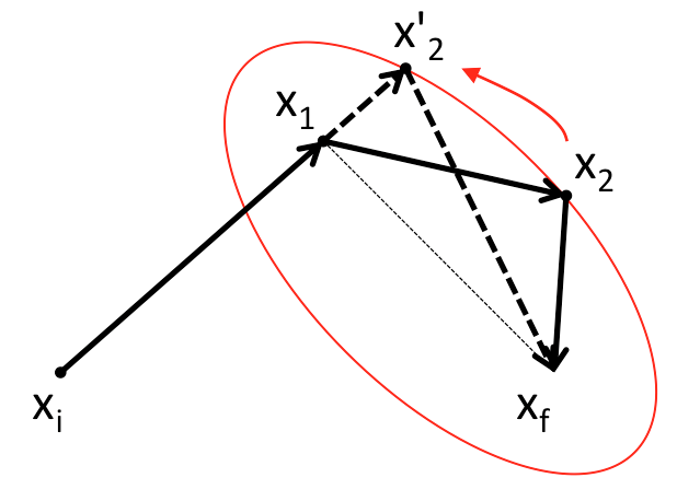
Figure 4: Relativistic PI with two intermediate steps.

We now give a geometrical proof that the symmetry-fixed two-step propagator (3.2) is given by the one-step propagator (31). This proof is to be understood within the “No-Over-Counting” definition of the path integral measure (9).

For any two points $\vec{x}_{1}$ and $\vec{x}_{2}$ in (3.2) one can distinguish three cases:

• If $\vec{x}_{1}$ is on the direct connection between $\vec{x}_{i}$ and $\vec{x}_{2}$, the step $\vec{x}_{1}$ does not contribute a new path to (3.2) and those paths do not contribute to $\int dx_{1}^{2}\int dx_{2}^{2}|_{NOC}$.

• If $\vec{x}_{2}$ is on the direct connection between $\vec{x}_{1}$ and $\vec{x}_{f}$, the step $\vec{x}_{2}$ does not contribute a new path to (3.2) and those paths do not contribute to $\int dx_{1}^{2}\int dx_{2}^{2}|_{NOC}$.

• If none of the above cases applies, one knows that the path $\vec{x}_{1}\rightarrow\vec{x}_{2}\rightarrow\vec{x}_{f}$ is equivalent (symmetry b) to the path $\vec{x}_{1}\rightarrow\vec{x}_{2}^{\prime}\rightarrow\vec{x}_{f}$ as indicated by the dashed lines in figure 4, where $\vec{x}_{2}^{\prime}$ is chosen such that $\vec{x}_{1}$ lies on the direct line between $\vec{x}_{i}$ and $\vec{x}_{2}^{\prime}$. As already shown, this different choice of $\alpha_{2}$ does not change the measure contributed by this path. Thus, the total path $\vec{x}_{i}\rightarrow\vec{x}_{1}\rightarrow\vec{x}_{2}\rightarrow\vec{x}_{f}$ is equivalent to the total path $\vec{x}_{i}\rightarrow\vec{x}_{1}\rightarrow\vec{x}_{2}^{\prime}\rightarrow\vec{x}_{f}$. Since $\vec{x}_{1}$ lies on the direct line between $\vec{x}_{i}$ and $\vec{x}_{2}^{\prime}$, one falls back to scenario 1).

Combining the outcome of those three possible scenarios one sees that the integration $\int dx_{1}^{2}\int dx_{2}^{2}|_{NOC}=\emptyset$. It only contains paths which are already present in the one-step integration $\int dx_{1}|_{NOC}$ . Thus one has shown that

$$K^{(2)}(\vec{x}_{i},\vec{x}_{f}) = K^{(1)}(\vec{x}_{i},\vec{x}_{f})|_{NOC}+K^{(2)}(\vec{x}_{i},\vec{x}_{f})|_{NOC}$$ (41)

$$= K^{(1)}(\vec{x}_{i},\vec{x}_{f})|_{NOC}+0$$

$$= {\mathcal{N}}\cdot K_{0}(x_{f}),$$

where the factor of $2\pi$ was absorbed in the normalization. Having shown that two intermediate steps are equivalent to one intermediate step one can repeat this procedure with $n$ steps and will always find that the propagator is given by (31). This also means that adding intermediate steps to the calculation of a propagator does not alter (31) and thus, the Kolmogorov relation holds trivially since there are no physically new intermediate points one can add. In anciant words: “There is nothing new under the sun”.

3.3 D dimensional case

Generalizing (35) to $n$ intermediate steps in $D$ dimensions is straight forward. The relation (41) holds also in this case, because one can set the angles $(\alpha_{i,1},...,\alpha_{i,N-1})$ such that new intermediate steps are on a straight line with the one-intermediate step case. Thus, the “nothing new theorem” holds also in $D\geq 2$ dimensions and the Kolmogorov relation for the relativistic point particle in $D$ dimensions becomes trivial.

3.4 A check: Three dimensional non-relativistic PI with two intermediate steps

Now, since it was shown that the entire relativistic path integral can be reduced to the one slicing case, one should revisit whether something similar happens in the non-relativistic case. Let’s consider a non-relativistic PI in three dimensions with two intermediate steps $\vec{x}_{i}\rightarrow\vec{x}_{1}\rightarrow\vec{x}_{2}\rightarrow\vec{x}_{f}$ as shown in figure 5.

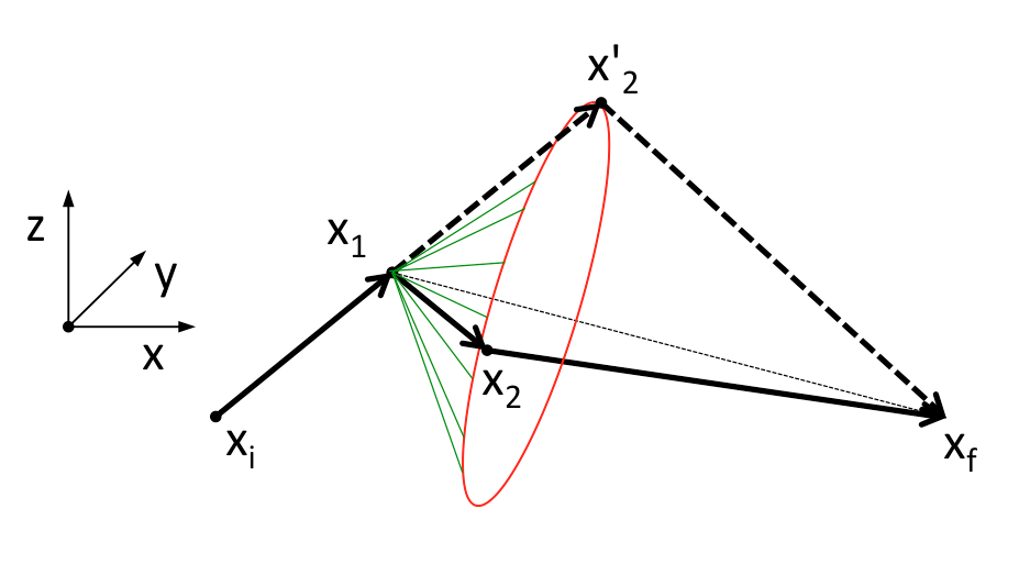
Figure 5: Non-Relativistic PI in three dimensions with two intermediate steps.

Let’s further consider the plane defined by the three points $\vec{x}_{i},\vec{x}_{1},\vec{x}_{f}$ and discuss the different scenarios that arise, when one chooses the second intermediate step $\vec{x}_{2}$.

• If the point $\vec{x}_{2}$ lies in the plane defined by $\vec{x}_{i},\vec{x}_{1},\vec{x}_{f}$, in some cases a direct overcounting can happen. This occurs when $\vec{x}_{2}$ lies on the continuation of the line $\vec{x}_{i}\rightarrow\vec{x}_{1}$ (indicated by the red dashed line in figure 5), this configuration is actually an overcounting, since it is already considered by a one-slicing path $\vec{x}_{i}\rightarrow\vec{x}_{2}\rightarrow\vec{x}_{f}$. This can happen, but it is actually numerically irrelevant since it corresponds to a one dimensional subset of the three dimensional volume $d^{3}x_{2}$.

• The same argument holds if $\vec{x}_{1}$ lies on the continuation of $\vec{x}_{f}\rightarrow\vec{x}_{2}$.

• If the point $\vec{x}_{2}$ lies outside of the plane defined by $\vec{x}_{i},\vec{x}_{1},\vec{x}_{f}$ it still can happen that it is connected to an overcounting by a local rotation. Due to the rotational invariance explained in figure 2 one can always choose the arbitrary angle $\alpha_{2}$ such that the transformed point $\vec{x}_{2}^{\prime}$ lies in the plane defined by $\vec{x}_{i},\vec{x}_{1},\vec{x}_{f}$. If this point $\vec{x}_{2}^{\prime}$ lies on the continuation of $\vec{x}_{i}\rightarrow\vec{x}_{1}$ one has an overcounting, otherwise not. All points $\vec{x}_{2}$, which correspond to an overcounting, lie on a cone who’s tip is the point $\vec{x}_{1}$, who’s symmetry axis is defined by the line $\vec{x}_{1}\rightarrow\vec{x}_{f}$, and who’s opening is given by the continuation of the line $\vec{x}_{i}\rightarrow\vec{x}_{1}$. This configuration is shown by the green surface in figure 5. Again the volume of this overcounting is two dimensional which is negligible with respect to the three dimensional volume of $d^{3}x_{2}$.

As a result of those three scenarios, one can conclude that there is some overcounting in the higher dimensional non-relativistic case with more than one slicing, but this overcounting is irrelevant since it is of lower dimension than the actual integral $d^{3}x_{2}$. Thus, in the non relativistic case one has to actually construct the complete PI by the use of the Kolmogorov relation. This is in contrast to the relativistic case, where the entire volume $d^{D}x_{2}$ turned out to be an overcounting. A generalization of this observation to higher number of dimensions and higher number of slicings is straight forward.

4 Discussion and conclusion

4.1 The Kolmogorov relation

It is interesting to discuss the results (35) and the D dimensional generalization of (41) in the context of the CK relation.

The usual way to state this relation in the non relativistic case is based on the fact that the one-step propagator $K_{NR}^{(1)}(x_{i},x_{f})$ takes the same form as the infinitesimal propagator $K_{NR}^{(0)}(x_{i},x_{f})$

$$K_{NR}^{(1)}(x_{i},x_{f})=K_{NR}^{(0)}(x_{i},x_{f}),$$ (42)

where,

$$K_{NR}^{(1)}(x_{i},x_{f})=\int d^{D}xK_{NR}^{(0)}(x_{i},x)K_{NR}^{(0)}(x,x_{f}).$$ (43)

This allows to construct the complete propagator $K(x_{i},x_{f})$ by iteration. Thus, (42) is also fulfilled by the complete propagator

$$K_{NR}(x_{i},x_{f})=\int d^{D}xK_{NR}(x_{i},x)K_{NR}(x,x_{f}).$$ (44)

In the relativistic case the infinitesimal propagator $K^{(0)}(x_{i},x_{f})$ differs from the one-step propagator $K^{(1)}(x_{i},x_{f})$

$$K^{(1)}(x_{i},x_{f})\neq K^{(0)}(x_{i},x_{f}),$$ (45)

where

$$K^{(1)}(x_{i},x_{f})=\int d^{D}x\Delta_{x}\cdot K^{(0)}(x_{i},x)K^{(0)}(x,x_{f})$$ (46)

and it seems hopeless to construct a PI from an iterative relation. As already seen, the rescue comes when one takes into account the issue of overcounting over symmetry-equivalent intermediate steps when gluing together additional infinitesimal propagators. By virtue of (41) one finds that the iteration actually converges at one intermediate step, since all additional intermediate steps can be identified as symmetry-equivalent to one intermediate step

$$K(x_{i},x_{f})\equiv K^{(n)}(x_{i},x_{f})=K^{(n-1)}(x_{i},x_{f})\quad{\mbox{for all}}\quad n\geq 2.$$ (47)

This is the building brick of the relativistic Kolmogorov relation (47) in analogy to the non-relativistic relation (42). The naive KG relation fails for the relativistic case since it ignores this issue of overcounting, and thus it is dominated by a summation over equivalent paths, which generates the “Tur Tur effect” Ende:1995 of increasingly deformed propagators as one continues to introduce intermediate steps.

4.2 Conclusion

The usual path integral formulation of relativistic quantum mechanics suffers from deep technical and conceptual problems. A first problem appears when one uses the Lagrangian action and calculates the propagator in a straight forward way. It turns out that such a calculation of the propagator gives a wrong result (see Appendix A). Even though, one can to some degree circumvent this particular problem by applying techniques such as renormalization procedures combined with semi-classical approximations Padmanabhan:1994 , or the introduction of auxiliary fields for the Hamiltonian action Brink:1976 ; Brink:1977 ; Fradkin:1991ci , there remains a much deeper conceptual problem. This second problem is that it is not understood how the combination of short time propagators $K^{(0)}$ gives long time propagators $K^{(n)}$ of the same functional form, in the spirit of the Chapman-Kolmogorov relation. This failure is typically taken as hint that it is impossible to consistently formulate the PI of the relativistic point particle and that one has to turn to QFT instead (at least if one does not want to redefine the usual notion of probability Jizba:2008 ; Jizba:2010pi ).

Those two long standing issues are resolved in this paper. For this purpose, we make notice of the symmetries (a), (b), and (c) which are present in this problem. Then, the usual PI measure is defined in a precise and explicit way (9), taking into account the issue of overcounting of equivalent and identical paths. Based on this, the relativistic one slicing propagator is calculated in a very simple and geometric way (35). The crucial step of the paper was then to show that it is indeed possible to consistently relate the n-slicing propagator to the one-slicing propagator by proving the relation (41). Thus, the one-step propagator (35) already gives the right result for the full propagator. This proof makes again heavy use of the symmetries and overcounting conditions discussed before. The main part of this paper concludes with a discussion on the Chapman-Kolmogorov relation and a conjecture on other quantum theories with general covariance.

It is hoped and believed that the presented work allows to finally reconcile the quantum mechanical PI formulation with the straight forward notion of a relativistic action (5).

Appendix A Propagator, direct calculation ignoring issue of overcounting

In this appendix, we present the derivation of Eq.(1). Let us consider the D-dimensional relativistic propagator between $\vec{x}_{i}\equiv\vec{x}_{0}=0$ and $\vec{x}_{f}\equiv\vec{x}_{n+1}$ fixed, for $n$-time slices, and for notational simplicity we adopt Euclidean metric.

$$K(0,\vec{x}_{f}) = \left[\prod_{j=1}^{n}\int d^{D}x_{j}\right]K(0,\vec{x}_{1})\ldots K(\vec{x}_{n},\vec{x}_{f})$$ (48)

$$= \left[\prod_{j=1}^{n}\int d^{D}x_{j}\right]e^{-M\sum_{l=0}^{n}|\vec{x}_{l+1}-\vec{x}_{l}|}.$$

Now, let us liberate the last point $\vec{x}_{n+1}$, by introducing a constraint via the identity $1=\int d^{D}x_{n+1}\delta(\vec{x}_{n+1}-\vec{x}_{f})$, as follows

$$K(0,\vec{x}_{f}) = \left[\prod_{j=1}^{n+1}\int d^{D}x_{j}\right]e^{-M\sum_{l=0}^{n}|\vec{x}_{l+1}-\vec{x}_{l}|}\times\delta(\vec{x}_{n+1}-\vec{x}_{f})$$ (49)

$$= \int\frac{d^{D}k}{(2\pi)^{D}}e^{-i\vec{k}\cdot\vec{x}_{f}}K_{n+1}(k,M).$$

Thus, the integrand in the above expression is nothing else but the Fourier transform of the propagator after $n$ time slices, thus corresponding to the multi-dimensional integral

$$K_{N+1}(k,M) = \left[\prod_{j=1}^{n+1}\int d^{D}x_{n}\right]$$ (50)

$$\times e^{-M\sum_{l=0}^{n}|\vec{x}_{l+1}-\vec{x}_{l}|+i\vec{k}\cdot\vec{x}_{n+1}}.$$

We begin by defining the new set of variables $\vec{y}_{0}=\vec{x}_{1}$, $\vec{y}_{1}=\vec{x}_{2}-\vec{x}_{1},\ldots$, $\vec{y}_{n}=\vec{x}_{n+1}-\vec{x}_{n}$. This set of equations can be inverted to yield

$$\vec{x}_{1} = \vec{y}_{0}$$

$$\vec{x}_{2} = \vec{y}_{0}+\vec{y}_{1}$$

$$\vdots$$

$$\vec{x}_{n+1} = \vec{y}_{0}+\vec{y}_{1}+\vec{y}_{2}+\ldots\vec{y}_{n}.$$ (51)

The Jacobian of this transformation is 1. Therefore, Eq.(50) can be expressed as

$$K_{n+1}(k,M) = \left[\prod_{j=0}^{n}\int d^{D}y_{j}\right]e^{-\sum_{l=0}^{n}(M|\vec{y}_{l}|+i\vec{k}\cdot\vec{y}_{l})}$$ (52)

$$= \left[K(k,M)\right]^{n+1}.$$

Here, $K(k,M)$ represents the Fourier transform of the zero-time-slice propagator, and thus can be expressed in D-dimensional spherical coordinates: $\rho=|\vec{y}_{n}|$, $d^{D}y_{n}=d\omega_{D}\rho^{D-1}d\rho$,

$$K(k,M) = \int d\omega_{D}\int_{0}^{\infty}d\rho\,\rho^{D-1}\,e^{-M\rho-i\,k\rho\cos\theta}.$$ (53)

Here, we use the recurrence property for the differential solid angle $d\omega_{D}=(\sin\theta)^{D-2}d\theta d\omega_{D-1}$. Considering the integral representation of the Bessel function of the first kind,

$$J_{\nu}(z)=\frac{(z/2)^{\nu}}{\Gamma(\nu+1/2)\Gamma(1/2)}\int_{0}^{\pi}e^{\pm iz\cos\theta}(\sin\theta)^{2\nu}d\theta,$$ (54)

the integral in Eq.(53) can be expressed as

$$K(k,M)=\frac{(2\pi)^{D/2}}{(k)^{D/2-1}}\int_{0}^{\infty}d\rho\,\rho^{D/2}\,e^{-M\rho}\,J_{D/2-1}(k\rho).$$ (55)

Substituting the expression for the solid angle in $D-1$-dimensions, $\omega_{D-1}=2\pi^{D/2-1/2}/\Gamma(D/2-1/2)$, and changing the variable of integration to $x=M\rho$, we have

$$K(k,M) = (2\pi)^{D/2}M^{-(D/2+1)}(k)^{1-D/2}$$ (56)

$$\times\int_{0}^{\infty}e^{-x}\,x^{D/2}\,J_{D/2-1}(k\,x/M).$$

The last integral is obtained analytically, thus giving

$$\int_{0}^{\infty}dx e^{-x}\,x^{D/2}\,J_{D/2-1}(k\,x/M)=\frac{2^{D/2}}{\sqrt{\pi}}\Gamma(D/2+1/2)$$ (57)

$$\times(k/M)^{D/2-1}\left(1+(k/M)^{2}\right)^{-D/2-1/2}.$$

Substituting into Eq.(56), we finally have

$$K(k,M)=\frac{(4\pi)^{D/2}}{\sqrt{\pi}}\frac{M\,\Gamma(D/2+1/2)}{\left(k^{2}+M^{2}\right)^{(D+1)/2}}.$$ (58)

Inserting this result into (52) one obtains the result stated in (2).

References

- (1) R. P. Feynman, Phys. Rev. 80, 440 (1950). doi:10.1103/PhysRev.80.440
- (2) C. Teitelboim, Phys. Rev. D 25, 12 (1982).
- (3) M. Henneaux and C. Teitelboim, Annals Phys. 143, 127 (1982). doi:10.1016/0003-4916(82)90216-0
- (4) I. H. Redmount and W. M. Suen, Int. J. Mod. Phys. A 8, 1629 (1993) doi:10.1142/S0217751X93000667 [gr-qc/9210019].
- (5) L. Brink, S. Deser, B. Zumino, P. Di Vecchia and P. S. Howe, Phys. Lett. B 64, 435 (1976).
- (6) L. Brink, P. Di Vecchia and P. S. Howe, Nucl. Phys. B 118, 76 (1977).
- (7) E. S. Fradkin and D. M. Gitman, Phys. Rev. D 44, 3230 (1991). doi:10.1103/PhysRevD.44.3230
- (8) H. Kleinert, “Path Integrals in Quantum Mechanics, Statistics, Polymer Physics, and Financial markets”, World Scientific Publishing, ISBN 978-981-4273-55-8.
- (9) T. Padmanabhan; Foundations of Physics, 25, 11 (1994); Padmanabhan, T. Found Phys (1994) 24: 1543. doi:10.1007/BF02054782.
- (10) P. Jizba and H. Kleinert, Phys. Rev. E 78, 031122 (2008) doi:10.1103/PhysRevE.78.031122.
- (11) P. Jizba and H. Kleinert, Phys. Rev. D 82, 085016 (2010) doi:10.1103/PhysRevD.82.085016 [arXiv:1007.3922 [hep-th]].
- (12) B. Koch, E. Munoz and I. Reyes, Phys. Rev. D 96, no. 8, 085011 (2017) doi:10.1103/PhysRevD.96.085011 [arXiv:1706.05386 [hep-th]].
- (13) L. D. Faddeev and V. N. Popov, Phys. Lett. 25B, 29 (1967). doi:10.1016/0370-2693(67)90067-6
- (14) B. Koch, E. Muñoz, I.A. Reyes, in preparation.
- (15) K. Fujikawa, Phys. Rev. Lett. 42, 1195 (1979). doi:10.1103/PhysRevLett.42.1195
- (16) M. Ende, Jim Knopf und Lukas der Lokomotivfuehrer; Omnibus Verlag, (1995), ISBN 3-570-20145-7.
- (17) M. Bañados and I. A. Reyes, Int. J. Mod. Phys. D 25, no. 10, 1630021 (2016) doi:10.1142/S0218271816300214 [arXiv:1601.03616 [hep-th]].