WUB/17-02
HU-EP-17/15
DAMTP-2017-22
Power corrections from decoupling of the charm quark

Abstract

Decoupling of heavy quarks at low energies can be described by means of an effective theory as shown by S. Weinberg in Ref. [1]. We study the decoupling of the charm quark by lattice simulations. We simulate a model, QCD with two degenerate charm quarks. In this case the leading order term in the effective theory is a pure gauge theory. The higher order terms are proportional to inverse powers of the charm quark mass $M$ starting at $M^{-2}$. Ratios of hadronic scales are equal to their value in the pure gauge theory up to power corrections. We show, by precise measurements of ratios of scales defined from the Wilson flow, that these corrections are very small and that they can be described by a term proportional to $M^{-2}$ down to masses in the region of the charm quark mass.

1 Introduction

In a field theory which contains light (mass-less) fields and fields of a heavy mass $M$, the functional integral over the latter can be performed resulting in an effective theory for the light fields which was formulated by Weinberg [1]. The action of the effective theory contains the action of the light fields (without the heavy fields) and an infinite number of non-renormalizable terms. The latter are suppressed by powers of $E/M$ at low energies $E\ll M$. Moreover, the non-renormalizable couplings do not contribute to the renormalization group equations of the renormalizable couplings of the light fields. This property holds for mass-independent renormalization schemes like the ${\rm\overline{MS\kern-0.50003pt}\kern 0.50003pt}$ scheme as shown in [1]. The heavy fields still affect the value of the renormalized couplings of the light fields through the decoupling relations, which result from the matching of the effective and the fundamental theory at low energies.

Assuming the validity of perturbation theory at the matching scale, the decoupling relations can be computed perturbatively. In the case of QCD and one heavy quark, such as the charm or the bottom quark, the decoupling relation for the renormalized strong coupling is known to four loops [1, 2, 3, 4]. The strong coupling of the five-flavor theory can be extracted in this way from the coupling computed non-perturbatively in the three-flavor theory using lattice simulations [5]. We remark that the decoupling relation for the strong coupling can be equivalently expressed as a relation between the $\Lambda$ parameters of the effective and the fundamental theory [6].

Simulations of QCD on the lattice are often carried out with three light sea quarks [7, 8, 9, 10, 11, 12]. The inclusion of a charm sea quark increases significantly the computational cost and introduces additional tuning to set the bare quark masses on a line of constant physics. Moreover, in the case of simulations with Wilson fermions, Symanzik O($a$) improvement requires the computation of coefficients which multiplies terms proportional to the bare quark masses in lattice units $am$ [13, 14]. The contribution of these terms is significant for the charm quark $am_{c}>0.3$ at the affordable lattice spacings $a>0.05{\rm fm}$. Some of these coefficients, like the one of the gluon action, are difficult to extract non-perturbatively. Relying on decoupling of the charm quark at low energies allows to simulate the cheaper and simpler effective theory with three flavors only.

The applicability of decoupling for the charm quark has to be justified. In [6] this was studied in a model, QCD with two heavy mass-degenerate quarks and no light quarks. The decoupling of the heavy quarks leave a pure gauge theory up to power corrections (which are due to the non-renormalizable interactions) at low energies. The latter were extracted by computing low energy quantities related to the Wilson flow [16, 17, 18, 19]. Ratios of two such quantities are insensitive to the matching of the gauge couplings, and after taking the continuum limit, can be compared to their counterparts in the pure gauge theory. The differences are due to the power corrections. By interpolating data obtained from simulations at quark masses ranging from $1/8$th up to one half of the charm quark mass with data from simulations of the pure gauge theory, the size of the power corrections due to one sea charm quark was estimated to be at the sub-percent level [6].

In [6] it was noted that the simulated masses were not large enough to see the leading behavior of the power corrections which start at $1/M^{2}$ in the effective theory. Instead a behavior more like $1/M$ was observed. In this article we study the same model as in [6] but extend the simulated quark masses to the charm quark mass and slightly above. Thus we can directly compute the size of the power corrections from decoupling of the charm quark. Furthermore we perform a non-perturbative test of the validity of the effective theory of decoupling for the charm quark. Our goal is to determine whether the leading power corrections in the inverse heavy quark mass behave in the charm region as $1/M^{2}$.

The article is organized as follows. In Sect. 2 we briefly review the theoretical framework of the effective theory of decoupling for QCD with two heavy mass-degenerate quarks (in the continuum). Sect. 3 presents the details of the Monte Carlo simulations of this model formulated on the lattice. The results for the ratios of low energy quantities are presented in Sect. 4 and their dependence on the heavy quark mass is compared to the effective theory prediction. The conclusions of our work are drawn in Sect. 5.

2 Decoupling

To avoid a multi-scale problem, we consider a simplified version of QCD, namely an $SU(3)$ Yang–Mills theory coupled to two degenerate heavy quarks. This allows us to perform simulations in relatively small volumes with very small lattice spacings, as we describe in Sect. 3. We briefly review the theoretical framework of decoupling specifically for our model. The fundamental theory is QCD with $N_{\mathrm{f}}=2$ mass-degenerate quarks. $\Lambda$ is the Lambda parameter in the ${\rm\overline{MS\kern-0.50003pt}\kern 0.50003pt}$ scheme and $M$ is the renormalization group invariant (RGI) mass of the heavy quarks. After decoupling of the heavy quarks, what is left is a pure gauge theory. Therefore, the Lagrangian of the effective theory valid at energies $E\ll M$ is given by [1, 20]

$${\mathcal{L}}_{\rm{dec}}={\mathcal{L}}_{\rm{YM}}+1/M^{2}\sum_{i}\omega_{i}\Phi_{i}+{\rm O}(\Lambda^{4}/M^{4})\,.$$ (1)

${\mathcal{L}}_{\rm{YM}}$ is the Lagrangian of the $SU(3)$ Yang–Mills (pure gauge) theory. Due to gauge invariance there are no fields of mass dimension equal to five. A complete set of fields of mass dimension equal to six is $\Phi_{1}=\mathrm{tr}\,\{D_{\mu}F_{\nu\rho}D_{\mu}F_{\nu\rho}\}$ and $\Phi_{2}=\mathrm{tr}\,\{D_{\mu}F_{\mu\rho}D_{\nu}F_{\nu\rho}\}$, where $F_{\mu\nu}$ is the $SU(3)$ field strength tensor and $D_{\mu}F_{\nu\rho}$ its covariant derivative.

At leading order the effective theory, eq. (1), is a Yang–Mills theory. It has only one free parameter, the renormalized gauge coupling. This coupling is fixed by matching the effective theory to the fundamental theory. Equivalently one can fix the $\Lambda$ parameter of the Yang–Mills theory, $\Lambda_{\rm YM}$, which becomes a function $\Lambda_{\rm YM}=\Lambda_{\mathrm{dec}}(M,\Lambda)$, see [6, 21]. Matching requires that low energy physical observables are the same in the two theories up to power corrections. Let us denote a low energy observable by $m^{\mathrm{had}}$ where, for example, it can represent a hadronic scale such as $1/\sqrt{t_{0}}$ [22] or $1/r_{0}$ [23]. After matching

$$m^{\mathrm{had}}(M)=m^{\mathrm{had}}_{\rm YM}+{\rm O}(\Lambda^{2}/M^{2})~{},$$ (2)

where $m^{\mathrm{had}}(M)$ is the hadronic scale in QCD with $N_{\mathrm{f}}=2$ heavy quarks of mass $M$ and $m^{\mathrm{had}}_{\rm YM}$ is the hadronic scale in the Yang–Mills theory. Note that $m^{\mathrm{had}}_{\rm YM}$ depends on $M$ through the matching, in particular $m^{\mathrm{had}}_{\rm YM}/\Lambda_{\rm YM}$ is a pure number independent of $M$. Therefore we consider two hadronic scales, $m^{\mathrm{had,1}}(M)$ and $m^{\mathrm{had,2}}(M)$, whose values in the Yang–Mills theory are $m_{\rm YM}^{\mathrm{had,1}}$ and $m_{\rm YM}^{\mathrm{had,2}}$ respectively. An immediate consequence of eq. (2) is

$$R(M)=\frac{m^{\mathrm{had,1}}(M)}{m^{\mathrm{had,2}}(M)}=\frac{m_{\rm YM}^{\mathrm{had,1}}}{m_{\rm YM}^{\mathrm{had,2}}}+{\rm O}(\Lambda^{2}/M^{2})\,.$$ (3)

The matching of the coupling is irrelevant for the ratios and we have direct access to the power corrections [24]. The effective theory of decoupling predicts that the ratios like in eq. (3) are equal to their value $R(M=\infty)$ in the Yang–Mills theory with a leading power correction in the inverse heavy quark mass given by

$$R(M)=R(\infty)+k\Lambda^{2}/M^{2}\,,$$ (4)

where $k$ is a parameter which depends on the hadronic scales which are taken to form the ratio. The goal of this work is to verify the behavior in eq. (4) and to establish whether it applies for masses around the charm quark mass.

3 Monte Carlo simulations

$\frac{T}{a}\times\left(\frac{L}{a}\right)^{3}$	$\beta$	$\kappa$	$a\mu$	$M/\Lambda$	$r_{0}/a$	$t_{0}/a^{2}$	MDUs
$120\times 32^{3}$	5.300	0.136457	0.024505	0.5900	–	4.174(13)	4300
$120\times 32^{3}$	5.500	0.1367749	0.018334	0.5900	8.77(15)	7.917(82)	8000
$192\times 48^{3}$	5.700	0.136687	0.013713	0.5900	–	14.40(10)	5800
$120\times 32^{3}$	5.500	0.1367749	0.039776	1.2800	8.010(62)	6.871(33)	8000
$192\times 48^{3}$	5.700	0.136687	0.029751	1.2800	–	12.668(39)	16200
$120\times 32^{3}$	5.500	0.1367749	0.077687	2.5000	7.392(62)	5.836(27)	8000
$192\times 48^{3}$	5.700	0.136687	0.058108	2.5000	–	10.916(38)	9000
$192\times 48^{3}$	5.600	0.136710	0.130949	4.8700	–	6.609(15)	2000
$120\times 32^{3}$	5.700	0.136698	0.113200	4.8703	9.123(57)	9.104(36)	17184
$192\times 48^{3}$	5.880	0.136509	0.087626	4.8700	11.946(55)	15.622(62)	23088
$192\times 48^{3}$	6.000	0.136335	0.072557	4.8700	14.34(10)	22.39(12)	22400
$192\times 48^{3}$	5.600	0.136710	0.155367	5.7781	–	6.181(11)	2096
$192\times 48^{3}$	5.700	0.136687	0.1343	5.7781	–	8.565(31)	2700
$120\times 32^{3}$	5.880	0.136509	0.103965	5.7781	–	14.916(93)	59888
$120\times 32^{3}$	6.100	–	–	$\infty$	6.345(13)	4.4329(32)	64000
$120\times 32^{3}$	6.340	–	–	$\infty$	9.029(77)	9.034(29)	20080
$120\times 24^{3}$	6.340	–	–	$\infty$	–	9.002(31)	60920
$192\times 48^{3}$	6.672	–	–	$\infty$	14.103(92)	21.924(81)	73920
$192\times 64^{3}$	6.900	–	–	$\infty$	18.93(15)	39.41(15)	160200

Table 1: Simulation parameters of our twisted mass and quenched ensembles. The columns show the lattice sizes, the gauge coupling $\beta=6/{g_{0}^{2}}$, the hopping parameter (for maximal twist), the twisted mass parameter, the ratio of the RGI mass to the $\Lambda$ parameter ($\infty$ for quenched), the scales $r_{0}/a$ (where it is measured) and $t_{0}/a^{2}$ and the total statistics in molecular dynamics units.

We simulate QCD with two mass-degenerate flavors of quarks ($N_{\mathrm{f}}=2$). Wilson’s plaquette gauge action [25] is employed in the the Yang-Mills sector and a doublet of quarks is realized either as standard or as twisted mass [26] Wilson quarks. In both cases a clover term [27, 13] with non-perturbatively determined improvement coefficient $c_{\rm sw}$ [28] is added. It is not needed for the $O(a)$ improvement of the twisted mass action at maximal twist, but was found to reduce the $O(a^{2})$ lattice artifacts, see e.g. [29].

The bare coupling $\beta$ of the gauge action was chosen such that the lattice spacings cover the range $0.023~{}{\rm fm}\lesssim a\lesssim 0.066~{}{\rm fm}$. The lattice spacing is determined from the hadronic scale $L_{1}$ [30, 31]. The scale $L_{1}/a$ is defined at vanishing quark mass, where the standard and twisted mass Wilson quark formulations are equivalent. Therefore, the lattice spacing for a given bare coupling $\beta$ is the same for both formulations. In order to obtain the scale $L_{1}$ in lattice units at a particular value of $\beta$, we fitted the data in Table 13 of [31] as it is explained there. The lattice spacing in physical units is estimated by rescaling the value $a=0.0486\,\mathrm{fm}$ at $\beta=5.5$ from [31] by the ratio of the $L_{1}/a$ values.

In order to resolve the short correlation lengths associated with the large quark masses that we aim at, we are forced to simulate at very small lattice spacings. Critical slowing down becomes a major obstacle which we alleviate by the implementation of open boundary conditions in the time direction [32]. The boundary improvement coefficients are kept at their tree-level values $c_{G}=1$ and $c_{F}=1$. The publicly available openQCD simulation program [33, 34] is used for our simulations.

We used standard O($a$) improved Wilson quarks to simulate at quark masses of approximately a factor $1/8$, $1/4$ and $1/2$ of the charm quark mass. The details of these simulations are given in [6, 21]. For the present work we also simulated twisted mass Wilson quarks at these quark masses. In addition, we also simulated directly at the charm quark mass and at one mass larger than that of the charm quark. In the simulations of twisted mass Wilson quarks, the hopping parameter $\kappa$ was set to its critical value in order to achieve maximal twist. The critical values were obtained from an interpolation of published data [31, 30, 35]. The twisted mass parameter $a\mu$ was chosen to correspond to certain values of $M/\Lambda$ listed in Table 1. More precisely, at a given value of the bare coupling the twisted mass parameter is set by

$$a\mu=\frac{M}{\Lambda}\,Z_{\rm P}(L_{1})\,\frac{\bar{m}(L_{1})}{M}\,\Lambda L_{1}\,\frac{a}{L_{1}}\,.$$ (5)

The pseudo-scalar renormalization constant at renormalization scale $L_{1}^{-1}$ computed in the Schrödinger Functional scheme $Z_{\rm P}(L_{1})=0.5184(53)$ (valid for $5.2\leq\beta\leq 6.0$), the relation between the running and the RGI mass $M/\bar{m}(L_{1})=1.308(16)$ and $\Lambda=310(20)\,{\rm MeV}$ are known from [31, 36]. We take $\Lambda L_{1}=0.649(45)$ from [37]. Some of the quantities entering eq. (5) have rather large errors. The dominant error comes from $\Lambda L_{1}$. Note that it is common to all our simulation points and amounts to a change in the target values of $M/\Lambda$. For the charm quark we set $M_{\rm c}/\Lambda=4.8700$, where we use the preliminary value $M_{\rm c}=1510\,{\rm MeV}$ of [38] which agrees with [39].

In order to determine the power corrections in eq. (3), we also simulate the pure gauge theory at values of the scales $t_{0}/a^{2}$ [22], $r_{0}/a$ [23] which are similar or larger.

Table 1 summarizes our twisted mass and quenched ensembles. At the large quark masses of our simulations, the system is close to a pure gauge theory, with similar finite volume effects. Our lattice volumes are such that $L/\sqrt{t_{0}}\geq 8$. We explicitly checked in the pure gauge theory that a volume $L/\sqrt{t_{0}}=8$ is large enough to exclude finite volume effects in the scales derived from the Wilson flow ($t_{0}$, $t_{c}$, $w_{0}$, see Sect. 4). In fact, we can rule out significant finite volume effects in all data which we use in the analysis in Sect. 4.

4 Results

On the ensembles generated with two flavors of O($a$) improved Wilson fermions reported in [6, 21] and those generated in the twisted mass simulations at maximal twist and the pure gauge simulations which are listed in Table 1, we measure the hadronic scales $\sqrt{t_{0}}$, $\sqrt{t_{c}}$ and $w_{0}$. They are defined from gauge fields smoothed by the Wilson flow [17, 18, 19] as follows. We denote by $E(x,t)$ the smoothed action density, where $t$ is the flow time of mass dimension $-2$, and introduce the dimensionless quantity

$${\cal E}(t)=t^{2}\left\langle E(x,t)\right\rangle\,.$$ (6)

At flow times $t>0$, $E(x,t)$ is a renormalized quantity [22, 40]. The reference scale $t_{0}$ is defined as in Ref. [22] by

$${\cal E}(t_{0})=0.3\,.$$ (7)

Similarly, the scale $t_{c}$ is defined by

$${\cal E}(t_{c})=0.2\,.$$ (8)

The numerical solutions to eq. (7) and eq. (8) are found by quadratic interpolation of the data of ${\cal E}(t)$. We use the clover (symmetric) definition of the action density $E$ on the lattice, cf. [22]. The scale $w_{0}$ is defined as in Ref. [41] by

$$w_{0}^{2}{\cal E}^{\prime}(w_{0}^{2})=0.3\,,$$ (9)

where ${\cal E}^{\prime}(t)=\frac{{\rm d}}{{\rm d}t}{\cal E}(t)$. The numerical solution to eq. (9) is found by first computing the symmetric finite differences of $t^{2}E(t)$ on each configuration and then by quadratic interpolation of the data. The error analysis is based on the method of Ref. [42] and takes into account the coupling to slow modes following Ref. [43]. We estimate the exponential autocorrelation time $\tau_{\rm exp}$ from the tail of the autocorrelation function of $t_{0}$. We use the ensembles at our largest masses, for which we perform simulations at our finest lattice spacings. As expected with open boundary conditions [32], the observed critical slowing down is compatible with a $\tau_{\rm exp}\propto a^{-2}$ behavior and from a least squares fit we obtain $\tau_{\rm exp}=-32(23)+17.4(2.8)\,t_{0}/a^{2}$ in molecular dynamics units (MDUs). The errors of the fit coefficients are given in parantheses. With periodic boundary conditions the autocorrelation times would be much larger, cf. [43] where an effective scaling proportional to $a^{-5}$ was observed.

We compute the ratios of hadronic scales

$$R=\sqrt{t_{c}/t_{0}}\; R=\sqrt{t_{0}}/w_{0}\,.$$ and (10)

In such ratios the bare coupling (or equivalently the lattice spacing) drops out. After taking the continuum limit we can directly compare the ratios in the $N_{\mathrm{f}}=2$ theory to their value in the pure gauge theory and so determine the size of the $1/M^{2}$ effects in eq. (4).

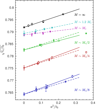
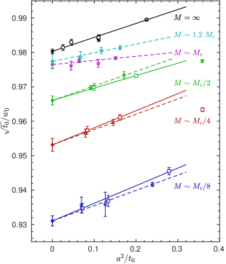
Figure 1: Combined continuum extrapolations. On the left, the ratio $\sqrt{t_{c}/t_{0}}$. On the right $\sqrt{t_{0}}/w_{0}$. We show data from twisted mass (pentagrams), standard Wilson (squares) and quenched (circles) simulations. For the second coarsest quenched lattice we performed a finite volume test and there are two data points overlapping. The lines represent the continuum extrapolations described in the text and the asterisks are the obtained continuum values.

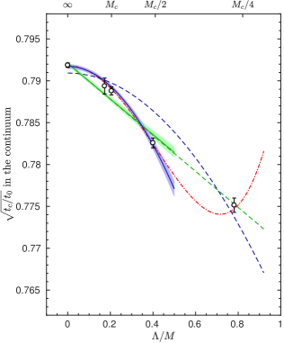
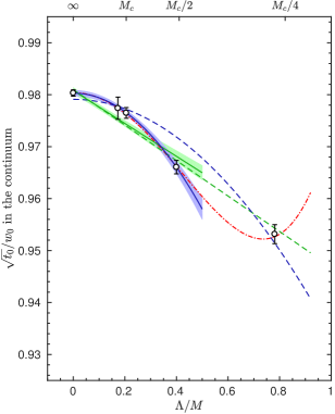
Figure 2: The continuum extrapolated values of $\sqrt{t_{c}/t_{0}}$ (left) and $\sqrt{t_{0}}/w_{0}$ (right) from the fit shown in Fig. 1 plotted against $\Lambda/M$. The line in the blue band is the effective theory prediction eq. (4) fitted through points from $M=\infty$ down to $M/\Lambda=2.5000$. The line in the green band is instead a fit linear in $\Lambda/M$. For comparison the dashed lines represent the quadratic (blue) and linear (green) fit through points from $M=\infty$ down to $M/\Lambda=1.2800$. Also shown by the dashed-dotted red line is a fit in this range adding to eq. (4) a next-to-leading correction term proportional to $\Lambda^{4}/M^{4}$.

To determine the values of the ratios in the continuum limit, we fit our data to $R(a,M/\Lambda,{\rm A})=R^{\rm cont}(M/\Lambda)+\frac{a^{2}}{t_{0}}c(M/\Lambda,{\rm A})$, where A is the action, “W” for Wilson, “tm” for twisted mass and “q” for quenched (pure gauge, $M=\infty$). The functional form is motivated by Symanzik’s effective theory for our actions. For a given mass $M/\Lambda$ we have two fit parameters (continuum value and slope) for cases where the calculation was performed with one action and three parameters (continuum value and two slopes) for cases with two lattice actions. We apply a cut, $a^{2}/t_{0}(M)<0.32$, to the data to be fitted. The data and the fits for $R=\sqrt{t_{c}/t_{0}}$ and $R=\sqrt{t_{0}}/w_{0}$ are shown in Fig. 1. The pentagrams represent the twisted mass data, the squares are the standard Wilson data and the circles are the pure gauge data. The lines represent fits: the dashed lines are the continuum extrapolations of the twisted mass data and the continued lines are the continuum extrapolations of the Wilson and of the quenched data. The asterisks represent the continuum extrapolated values $R^{\rm cont}(M/\Lambda)$. The data is described very well by the fits and the continuum values are very stable under changes in the fitting procedure, such as removing some of the data points, or changes in the cut in $a^{2}/t_{0}(M)$. Moreover, a global fit that models the $M$ dependence of the slopes yields compatible values. Although the global fit has less parameters, we prefer the individual fits since they yield statistically independent continuum values.

$M/\Lambda$	$\infty$	5.7781	4.87	2.50	1.28	0.59
$\sqrt{t_{c}/t_{0}}$	0.7919(3)	0.7894(9)	0.7888(5)	0.7826(6)	0.7751(9)	0.7643(6)
$\sqrt{t_{0}}/w_{0}$	0.9803(6)	0.9774(21)	0.9765(10)	0.9661(13)	0.9532(18)	0.9311(15)
$r_{0}/\sqrt{t_{0}}$	3.013(17)	-	3.022(29)	2.988(35)	3.043(71)	3.050(64)

Table 2: The values of various dimensionless ratios in the continuum limit for several values of the quark mass.

The continuum values $R^{\rm cont}(M/\Lambda)$ obtained from the fit are summarized in Table 2 and are plotted in Fig. 2 against $\Lambda/M$. The relative effect of a single charm quark compared to pure gauge theory can be estimated by $1/2[R^{\rm cont}(M_{\rm c})-R^{\rm cont}(\infty)]/R^{\rm cont}(\infty)$. This effect is very small, it is $-0.00196(37)$ for $R=\sqrt{t_{c}/t_{0}}$ and $-0.00194(59)$ for $R=\sqrt{t_{0}}/w_{0}$. In Fig. 2 the line in the blue band represents the effective theory prediction eq. (4), where the coefficient $k$ of the $(\Lambda/M)^{2}$ term is determined by a fit that includes data down to $M/\Lambda=2.50$. Our data are very well described by eq. (4). A fit to a behavior of the power corrections linear in $M^{-1}$ is shown by the line in the green band. A linear behavior in $1/M$ was observed in the data for masses smaller than half of the charm quark mass [6, 21]. While adding the new data for larger masses cannot exclude the $M^{-1}$ behavior completely, this fit is far worse than the one with $M^{-2}$ corrections. The fitted values of the coefficients $k$ and the $\chi^{2}$ values per degree of freedom of the fits are listed in Table 3 . The second error of $k$ is systematic and is given by the difference between fits where the lowest mass included in the fit is $M_{\rm c}$ or $M_{\rm c}/2$.

$R$	fits down to $M_{\rm c}/2$			fits down to $M_{\rm c}/4$
	$k$	$\chi^{2}_{\rm quad}/{\rm dof}$	$\chi^{2}_{\rm lin}/{\rm dof}$	$\chi^{2}_{\rm quad}/{\rm dof}$	$\chi^{2}_{\rm lin}/{\rm dof}$
$\sqrt{t_{c}/t_{0}}$	-0.058(04)(16)	1.75 / 2	9.55 / 2	65.76 / 3	9.61 / 3
$\sqrt{t_{0}}/w_{0}$	-0.089(09)(03)	0.02 / 2	8.54 / 2	27.31 / 3	9.54 / 3
$r_{0}/\sqrt{t_{0}}$	-0.14(24)(37)	0.25 / 1	0.42 / 1	0.78 / 2	0.79 / 2

Table 3: The $\chi^{2}$ values of the quadratic eq. (4) and linear fits in $\Lambda/M$ for different ratios shown in Figure 2 and on the right plot in Figure 3. We perform two types of fits, the first through the $M=\infty$ and $M_{c}/2$ data points and the second extending down to the $M_{c}/4$ data points. For the first type of fits we list the values of the coefficients $k$ of the $(\Lambda/M)^{2}$ term in eq. (4). The first error is statistical and the second is systematic.

In Fig. 2 we also show the fits to the data down to masses corresponding to $M_{\rm c}/4$. They are represented by the dashed lines, blue for the quadratic and green for the linear fit. While the linear fit is almost unchanged with respect to the linear fit down to $M_{\rm c}/2$, the quadratic fit is clearly excluded. Still the quadratic fit to the points down to $M_{\rm c}/2$ has much better $\chi^{2}$ values per degree of freedom than the linear fit down to $M_{\rm c}/4$, see Table 3 . These results demonstrate that the linear behavior is disfavored only when the data for masses smaller than $M_{\rm c}/2$ are excluded from the fits. The data then begin to show the leading quadratic behavior which is expected from the effective theory for large enough masses. This conclusion is further supported by the dashed-dotted lines shown in Fig. 2. They represent a fit down to $M_{\rm c}/4$ when a next-to-leading correction term $\Lambda^{4}/M^{4}$ (whose coefficient is fitted) is added to the leading behavior of eq. (4). This fit has very good $\chi^{2}$ values per degree of freedom: $0.49/2$ for $R=\sqrt{t_{c}/t_{0}}$ and $0.11/2$ for $R=\sqrt{t_{0}}/w_{0}$. It deviates substantially from the fit to the leading behavior down to $M_{\rm c}/2$ only for masses smaller than $M_{\rm c}/2$.

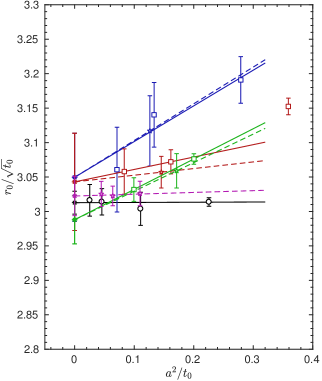
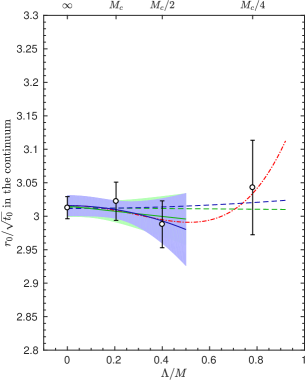
Figure 3: Combined continuum extrapolations of the ratio $r_{0}/\sqrt{t_{0}}$ (left) and the mass dependence of the continuum values (right). The symbols and colors are chosen as in Fig. 1 and Fig. 2.

In order to appreciate the precision that can be reached with flow quantities, we also present the corresponding results for the ratio $R=r_{0}/\sqrt{t_{0}}$ including the Sommer-scale $r_{0}$ [23] extracted from Wilson loops. For the measurements of Wilson loops we use the wloop package which implements the method of [44]. This amounts to firstly smearing all gauge links (for the temporal links this means a choice of the static action) and subsequently measuring the Wilson loops where the initial and final line of gauge links are smeared using up to four levels of spatial HYP smearing [45]. This allows us to extract the static-quark potential $a\,V(r)$ very reliably by solving a generalized eigenvalue problem [46]. The static force $F(r)=V^{\prime}(r)$ can then be used to measure the hadronic scale $r_{0}$ defined implicitly through [23]

$$r_{0}^{2}F(r_{0})=1.65\,.$$ (11)

Even a careful state of the art determination of $r_{0}$ does not yield a precision high enough to resolve the power corrections we are interested in, as can be seen in Fig. 3. We note that the coefficient $k$ of the $(\Lambda/M)^{2}$ term in eq. (4) depends on the observables used to form the ratio.

5 Conclusions

In this work we simulated a model, QCD with two heavy mass-degenerate quarks. At low energies this theory is described by an effective theory which is a pure gauge theory up to power corrections in the inverse heavy quark mass. By comparing ratios of low energy physical quantities computed in both theories and extrapolated to the continuum limit, we could determine the size of the power corrections. They have been found to be very small. We are now confident that the effects of neglecting the charm quark in $N_{\mathrm{f}}=2+1$ simulations is far below a percent in dimensionless low-energy quantities. The power corrections are expected for sufficiently large heavy quark masses to be proportional to the square of the inverse quark mass, see eq. (4). Our data shown in Fig. 2 follow very well this expectation down to masses equal to half of the charm quark mass. A behavior linear in the inverse quark mass, which is possible for masses outside the range of validity of the effective theory, is strongly disfavored by the data.

In order to achieve a stronger conclusion and find the range of quark masses where the linear behavior can be completely excluded, the statistics of our simulations should be increased and larger quark masses up to the bottom quark mass be simulated. The resources needed to carry this out are beyond our computational budget. We emphasize that the computational resources used to produce the data for this article amount to a large scale project already. Simulating with a yet larger statistical precision and heavier quark masses would require a computational effort which is comparable to simulations with light sea quarks and are therefore beyond the scope of this model calculation.

Acknowledgements. The study of decoupling was initiated by Rainer Sommer whom we thank for many useful discussions and for his valuable comments on the manuscript. We also thank Jacob Finkenrath for a check on our measurements. The authors gratefully acknowledge the Gauss Centre for Supercomputing (GCS) for providing computing time for a GCS Large-Scale Project on the GCS share of the supercomputer JUQUEEN at Jülich Supercomputing Centre (JSC). GCS is the alliance of the three national supercomputing centres HLRS (Universität Stuttgart), JSC (Forschungszentrum Jülich), and LRZ (Bayerische Akademie der Wissenschaften), funded by the German Federal Ministry of Education and Research (BMBF) and the German State Ministries for Research of Baden-Württemberg (MWK), Bayern (StMWFK) and Nordrhein-Westfalen (MIWF). GM acknowledges support from the Herchel Smith Fund at the University of Cambridge. This work is supported by the Deutsche Forschungsgemeinschaft in the SFB/TR 55.

References

- [1] S. Weinberg, Effective Gauge Theories, Phys. Lett. B91 (1980) 51–55. doi:10.1016/0370-2693(80)90660-7.
- [2] W. Bernreuther, W. Wetzel, Decoupling of Heavy Quarks in the Minimal Subtraction Scheme, Nucl. Phys. B197 (1982) 228–236, [Erratum: Nucl. Phys.B513,758(1998)]. doi:10.1016/0550-3213(82)90288-7,10.1016/S0550-3213(97)00811-0.
- [3] K. G. Chetyrkin, J. H. Kühn, C. Sturm, QCD decoupling at four loops, Nucl. Phys. B744 (2006) 121–135. arXiv:hep-ph/0512060, doi:10.1016/j.nuclphysb.2006.03.020.
- [4] Y. Schröder, M. Steinhauser, Four-loop decoupling relations for the strong coupling, JHEP 01 (2006) 051. arXiv:hep-ph/0512058, doi:10.1088/1126-6708/2006/01/051.
- [5] M. Bruno, M. Dalla Brida, P. Fritzsch, T. Korzec, A. Ramos, S. Schaefer, H. Simma, S. Sint, R. Sommer, The strong coupling from a nonperturbative determination of the parameter in three-flavor QCD, Phys. Rev. Lett. 119 (2017) 102001. arXiv:1706.03821, doi:10.1103/PhysRevLett.119.102001.
- [6] M. Bruno, J. Finkenrath, F. Knechtli, B. Leder, R. Sommer, Effects of Heavy Sea Quarks at Low Energies, Phys. Rev. Lett. 114 (10) (2015) 102001. arXiv:1410.8374, doi:10.1103/PhysRevLett.114.102001.
- [7] H.-W. Lin, et al., First results from 2+1 dynamical quark flavors on an anisotropic lattice: Light-hadron spectroscopy and setting the strange-quark mass, Phys. Rev. D79 (2009) 034502. arXiv:0810.3588, doi:10.1103/PhysRevD.79.034502.
- [8] S. Aoki, et al., Physical Point Simulation in 2+1 Flavor Lattice QCD, Phys. Rev. D81 (2010) 074503. arXiv:0911.2561, doi:10.1103/PhysRevD.81.074503.
- [9] W. Bietenholz, et al., Tuning the strange quark mass in lattice simulations, Phys. Lett. B690 (2010) 436–441. arXiv:1003.1114, doi:10.1016/j.physletb.2010.05.067.
- [10] R. Arthur, et al., Domain Wall QCD with Near-Physical Pions, Phys. Rev. D87 (2013) 094514. arXiv:1208.4412, doi:10.1103/PhysRevD.87.094514.
- [11] M. Bruno, et al., Simulation of QCD with N 2 1 flavors of non-perturbatively improved Wilson fermions, JHEP 02 (2015) 043. arXiv:1411.3982, doi:10.1007/JHEP02(2015)043.
- [12] G. S. Bali, E. E. Scholz, J. Simeth, W. Söldner, Lattice simulations with improved Wilson fermions at a fixed strange quark mass, Phys. Rev. D94 (7) (2016) 074501. arXiv:1606.09039, doi:10.1103/PhysRevD.94.074501.
- [13] M. Lüscher, S. Sint, R. Sommer, P. Weisz, Chiral symmetry and O(a) improvement in lattice QCD, Nucl. Phys. B478 (1996) 365–400. arXiv:hep-lat/9605038, doi:10.1016/0550-3213(96)00378-1.
- [14] T. Bhattacharya, R. Gupta, W. Lee, S. R. Sharpe, J. M. S. Wu, Improved bilinears in lattice QCD with non-degenerate quarks, Phys. Rev. D73 (2006) 034504. arXiv:hep-lat/0511014, doi:10.1103/PhysRevD.73.034504.
- [15] A. G. Grozin, M. Hoeschele, J. Hoff, M. Steinhauser, M. Hoschele, J. Hoff, M. Steinhauser, Simultaneous decoupling of bottom and charm quarks, JHEP 09 (2011) 066. arXiv:1107.5970, doi:10.1007/JHEP09(2011)066.
- [16] M. F. Atiyah, R. Bott, The Yang-Mills equations over Riemann surfaces, Phil. Trans. Roy. Soc. Lond. A308 (1982) 523–615.
- [17] R. Narayanan, H. Neuberger, Infinite N phase transitions in continuum Wilson loop operators, JHEP 03 (2006) 064. arXiv:hep-th/0601210, doi:10.1088/1126-6708/2006/03/064.
- [18] M. Lüscher, Trivializing maps, the Wilson flow and the HMC algorithm, Commun. Math. Phys. 293 (2010) 899–919. arXiv:0907.5491, doi:10.1007/s00220-009-0953-7.
- [19] R. Lohmayer, H. Neuberger, Continuous smearing of Wilson Loops, PoS LATTICE2011 (2011) 249. arXiv:1110.3522.
- [20] S. Weinberg, Phenomenological lagrangians, Physica A96 (1979) 327.
- [21] A. Athenodorou, M. Bruno, J. Finkenrath, F. Knechtli, B. Leder, M. Marinkovic, R. Sommer, The decoupling of heavy sea quarks, in preparation.
- [22] M. Lüscher, Properties and uses of the Wilson flow in lattice QCD, JHEP 08 (2010) 071, [Erratum: JHEP03,092(2014)]. arXiv:1006.4518, doi:10.1007/JHEP08(2010)071,10.1007/JHEP03(2014)092.
- [23] R. Sommer, A New way to set the energy scale in lattice gauge theories and its applications to the static force and alpha-s in SU(2) Yang-Mills theory, Nucl. Phys. B411 (1994) 839–854. arXiv:hep-lat/9310022, doi:10.1016/0550-3213(94)90473-1.
- [24] F. Knechtli, J. Finkenrath, B. Leder, A. Athenodorou, M. Bruno, R. Sommer, M. Marinkovic, Physical and cut-off effects of heavy sea quarks, PoS LATTICE2014 (2014) 288. arXiv:1411.1239.
- [25] K. G. Wilson, Confinement of Quarks, Phys. Rev. D10 (1974) 2445–2459, [,45(1974)]. doi:10.1103/PhysRevD.10.2445.
- [26] R. Frezzotti, P. A. Grassi, S. Sint, P. Weisz, Lattice QCD with a chirally twisted mass term, JHEP 08 (2001) 058. arXiv:hep-lat/0101001.
- [27] B. Sheikholeslami, R. Wohlert, Improved Continuum Limit Lattice Action for QCD with Wilson Fermions, Nucl. Phys. B259 (1985) 572. doi:10.1016/0550-3213(85)90002-1.
- [28] K. Jansen, R. Sommer, O() improvement of lattice QCD with two flavors of Wilson quarks, Nucl. Phys. B530 (1998) 185–203, [Erratum: Nucl. Phys.B643,517(2002)]. arXiv:hep-lat/9803017, doi:10.1016/S0550-3213(98)00396-4,10.1016/S0550-3213(02)00624-7.
- [29] P. Dimopoulos, H. Simma, A. Vladikas, Quenched B(K)-parameter from Osterwalder-Seiler tmQCD quarks and mass-splitting discretization effects, JHEP 07 (2009) 007. arXiv:0902.1074, doi:10.1088/1126-6708/2009/07/007.
- [30] B. Blossier, M. Della Morte, P. Fritzsch, N. Garron, J. Heitger, H. Simma, R. Sommer, N. Tantalo, Parameters of Heavy Quark Effective Theory from Nf=2 lattice QCD, JHEP 09 (2012) 132. arXiv:1203.6516, doi:10.1007/JHEP09(2012)132.
- [31] P. Fritzsch, F. Knechtli, B. Leder, M. Marinkovic, S. Schaefer, R. Sommer, F. Virotta, The strange quark mass and Lambda parameter of two flavor QCD, Nucl. Phys. B865 (2012) 397–429. arXiv:1205.5380, doi:10.1016/j.nuclphysb.2012.07.026.
- [32] M. Lüscher, S. Schaefer, Lattice QCD without topology barriers, JHEP 1107 (2011) 036. arXiv:1105.4749, doi:10.1007/JHEP07(2011)036.
- [33] http://luscher.web.cern.ch/luscher/openQCD/.
- [34] M. Lüscher, S. Schaefer, Lattice QCD with open boundary conditions and twisted-mass reweighting, Comput.Phys.Commun. 184 (2013) 519–528. arXiv:1206.2809, doi:10.1016/j.cpc.2012.10.003.
- [35] P. Fritzsch, N. Garron, J. Heitger, Non-perturbative tests of continuum HQET through small-volume two-flavour QCD, JHEP 01 (2016) 093. arXiv:1508.06938, doi:10.1007/JHEP01(2016)093.
- [36] M. Della Morte, R. Hoffmann, F. Knechtli, J. Rolf, R. Sommer, I. Wetzorke, U. Wolff, Non-perturbative quark mass renormalization in two-flavor QCD, Nucl. Phys. B729 (2005) 117–134. arXiv:hep-lat/0507035, doi:10.1016/j.nuclphysb.2005.09.028.
- [37] M. Della Morte, R. Frezzotti, J. Heitger, J. Rolf, R. Sommer, U. Wolff, Computation of the strong coupling in QCD with two dynamical flavors, Nucl. Phys. B713 (2005) 378–406. arXiv:hep-lat/0411025, doi:10.1016/j.nuclphysb.2005.02.013.
- [38] J. Heitger, G. M. von Hippel, S. Schaefer, F. Virotta, Charm quark mass and D-meson decay constants from two-flavour lattice QCD, PoS LATTICE2013 (2014) 475. arXiv:1312.7693.
- [39] C. Patrignani, et al., Review of Particle Physics, Chin. Phys. C40 (10) (2016) 100001. doi:10.1088/1674-1137/40/10/100001.
- [40] M. Lüscher, P. Weisz, Perturbative analysis of the gradient flow in non-abelian gauge theories, JHEP 02 (2011) 051. arXiv:1101.0963, doi:10.1007/JHEP02(2011)051.
- [41] S. Borsanyi, S. Dürr, Z. Fodor, C. Hoelbling, S. D. Katz, S. Krieg, T. Kurth, L. Lellouch, T. Lippert, C. McNeile, K. K. Szabo, High-precision scale setting in lattice QCD, JHEP 09 (2012) 010. arXiv:1203.4469, doi:10.1007/JHEP09(2012)010.
- [42] U. Wolff, Monte Carlo errors with less errors, Comput.Phys.Commun. 156 (2004) 143–153. arXiv:hep-lat/0306017, doi:10.1016/S0010-4655(03)00467-3,10.1016/j.cpc.2006.12.001.
- [43] S. Schaefer, R. Sommer, F. Virotta, Critical slowing down and error analysis in lattice QCD simulations, Nucl.Phys. B845 (2011) 93–119. arXiv:1009.5228, doi:10.1016/j.nuclphysb.2010.11.020.
- [44] M. Donnellan, F. Knechtli, B. Leder, R. Sommer, Determination of the Static Potential with Dynamical Fermions, Nucl.Phys. B849 (2011) 45–63. arXiv:1012.3037, doi:10.1016/j.nuclphysb.2011.03.013.
- [45] A. Hasenfratz, F. Knechtli, Flavor symmetry and the static potential with hypercubic blocking, Phys.Rev. D64 (2001) 034504. arXiv:hep-lat/0103029, doi:10.1103/PhysRevD.64.034504.
- [46] B. Blossier, M. Della Morte, G. von Hippel, T. Mendes, R. Sommer, On the generalized eigenvalue method for energies and matrix elements in lattice field theory, JHEP 04 (2009) 094. arXiv:0902.1265, doi:10.1088/1126-6708/2009/04/094.