Probing the shape and internal structure of dark matter halos with the halo-shear-shear three-point correlation function

Abstract

Weak lensing three-point statistics are powerful probes of the structure of dark matter halos. We propose to use the correlation of the positions of galaxies with the shapes of background galaxy pairs, known as the halo-shear-shear correlation (HSSC), to measure the mean halo ellipticity and the abundance of subhalos in a statistical manner. We run high-resolution cosmological $N$-body simulations and use the outputs to measure the HSSC for galaxy halos and cluster halos. Non-spherical halos cause a characteristic azimuthal variation of the HSSC, and massive subhalos in the outer region near the virial radius contribute to $\sim 10\%$ of the HSSC amplitude. Using the HSSC and its covariance estimated from our $N$-body simulations, we make forecast for constraining the internal structure of dark matter halos with future galaxy surveys. With 1000 galaxy groups with mass greater than $10^{13.5}\,h^{-1}M_{\odot}$, the average halo ellipticity can be measured with an accuracy of ten percent. A spherical, smooth mass distribution can be ruled out at a $\sim 5\sigma$ significance level. The existence of subhalos whose masses are in 1-10 percent of the main halo mass can be detected with $\sim 10^{4}$ galaxies/clusters. We conclude that the HSSC provides valuable information on the structure of dark halos and hence on the nature of dark matter.

1 INTRODUCTION

An array of astronomical observations suggest that ordinary matter accounts for only about twenty percent of the mass content of the Universe. The rest consists of some unknown substitute called dark matter. Measurements of temperature anisotropies in the cosmic microwave background (CMB) suggest the existence of dark matter at $\sim 50\sigma$ significance level, and also that dark matter should be non-baryonic (e.g. Planck Collaboration et al., 2016). Although the nature of dark matter is still unknown, currently available astronomical data of large-scale structure of the comoving lengthscale of $\lower 2.15277pt\hbox{$\;\buildrel>\over{\sim}\;$}10\,{\rm Mpc}$ are consistent with a simple model of cold dark matter (CDM) that posits that dark matter is made of stable, collisionless, and non-relativistic particles (e.g. Tegmark et al., 2006).

There appear to exist a few discrepancies between the theoretical prediction of the standard CDM model and observations of galactic-size objects (see, e.g. Weinberg et al., 2015, for a short review). Such a “small-scale crisis” of the CDM model can be resolved by modifying the particle nature of dark matter. For example, in warm dark matter (WDM) models, the primordial density perturbations at small length scales are suppressed owing to free-streaming of dark matter particles (e.g. Dodelson & Widrow, 1994). Self-interacting dark matter (SIDM) model is another alternative. If dark matter is made of collisional particles (e.g. Spergel & Steinhardt, 2000), dark halos are rounder, and typically have a density profile with a constant density “core" that appears to be in agreement with observations of rotation curves of galaxies (e.g. Kaplinghat et al., 2016). A promising way to discriminate the variants of dark matter models is to directly probe the structure of dark matter halos.

Gravitational lensing provides a unique physical method to probe matter distribution in and around galaxies. Although the lensing effect on individual source galaxies is expected to be small, statistical analyses of a large number of sources enable us to reconstruct the matter density distribution in an unbiased way. In particular, cross-correlation of large-scale structure tracers such as galaxies and galaxy clusters with shapes of background galaxies, measured by a stacking method, can be used to infer the average total matter distribution around galaxies (e.g. Brainerd et al., 1996; Hudson et al., 1998; Guzik & Seljak, 2002; Hoekstra et al., 2004; Mandelbaum et al., 2006a) and galaxy clusters (e.g. Mandelbaum et al., 2006c; Johnston et al., 2007; Okabe et al., 2013; Covone et al., 2014). The gravitational lensing effects have been detected and extensively studied also for individual galaxy clusters (e.g. Broadhurst et al., 2005; Oguri et al., 2012; Hoekstra et al., 2012; Applegate et al., 2014; Battaglia et al., 2016). Such measurements play a central role in constraining the spherically averaged density profile, but it is difficult to extract more information about the fine structure of dark matter halos. Numerical simulations predict that dark matter halos are triaxial (e.g. Jing & Suto, 2002) and have abundant substructures (e.g. Tormen et al., 1998). Recent simulations for a variant of dark matter models show that the structure of dark halos are useful to constrain the nature of dark matter (e.g. Peter et al., 2013; Elahi et al., 2014).

The shape of dark matter halos has been investigated with stacked weak lensing analysis so far. There exist various studies to measure the projected ellipticity of surface mass density around galaxy-sized halos (e.g. Hoekstra et al., 2004; Mandelbaum et al., 2006b; Parker et al., 2007; van Uitert et al., 2012; Schrabback et al., 2015), whereas recent galaxy-imaging observations allow us to study the shape of more massive halos, galaxy groups (Clampitt & Jain, 2016; van Uitert et al., 2017) and galaxy clusters (Evans & Bridle, 2009). Most previous lensing measurements of the halo shape require some proxy of orientation of the principal axes in surface mass density around lensing objects. On galaxy scales, it is commonly assumed that a galaxy resides perfectly at the center of the dark halo. For more massive objects, such as galaxy groups and clusters, one may expect that the distribution of member galaxies will follow the mass distribution. However, there also exists some observational evidence that central massive galaxies and their dark halos are not aligned (Okumura et al., 2009) and that there is only weak correlation between the dark mass ellipticity and that of the distribution of the member galaxies (Oguri et al., 2010). Interestingly, recent hydrodynamics simulations show that the light distribution does not follow the underlying mass distribution in halos of galaxies and clusters (e.g. Velliscig et al., 2015; Chisari et al., 2017). It is still difficult to interpret the results of conventional stacked weak lensing analysis appropriately, without knowing the galaxy-halo misalignment a priori.

In this paper, we extend the method of stacked lensing to probe the internal structure of dark matter halos. We consider a three-point correlation defined by the correlation of the shapes of background-galaxy pairs around the positions of lensing galaxies (halos). Throughout this paper, we refer to this three-point correlation as halo-shear-shear correlation (HSSC). A great advantage of using the HSSC is that statistical measurement can be done without relying on the light distribution of central galaxies or on the spatial distribution of the member galaxies. Simon et al. (2012) use an isolated lens model to show that the HSSC, without using luminous tracers, can probe the halo ellipticity. More recently, Adhikari et al. (2015) propose a statistical method to measure the HSSC and to constrain the mean ellipticity of galaxy-size halos without using any information about the halo orientation. The HSSC can be applied to study more massive objects like galaxy groups and clusters, and it will be more successful than galaxy-size halos since the lensing signal is expected to be stronger. Nevertheless, it still remains uncertain if the HSSC can probe the average ellipticity of group and cluster halos in practice. The standard CDM model predicts that numerous dark substructures are expected to exist. They can induce possible anisotropic signals in the HSSC. In addition, projected uncorrelated structures along a line of sight can also affect the observed HSSC. To study these effects on the HSSC simultaneously, we use high-resolution $N$-body simulations as one of the best approaches at present. Observationally, HSSC has been already detected with a high significance by recent weak lensing surveys (e.g. Simon et al., 2008, 2013), but these measurements have still focused on the large-scale three-point correlation. Since ongoing and upcoming galaxy surveys hold promise for measuring the HSSC with a high statistical significance on scales down to virial radii of group- and cluster-sized halos, it is important and timely to develop an accurate theoretical model of the HSSC induced by the internal structures of dark halos. For this purpose, we use realistic halo catalogs from high-resolution N-body simulations to examine the ability of HSSC to detect or measure halo ellipticity. We also study the impact of substructures and projected large-scale structures along a line of sight on the HSSC for the first time. Note that our analysis focuses on the HSSC for massive galaxies and galaxy clusters and hence is complementary to the work of Adhikari et al. (2015).

This paper is organized as follows. In Section 2, we summarize the basics of weak lensing and lensing statistics used in this paper. We explain the details of our lensing simulation and the methodology to estimate lensing statistics in Section 3. In Section 4, we show how the HSSC will be sensitive to halo ellipticity and presence of substructures, and study the projection effect along a line of sight. We then quantify the information content in the HSSC on the internal structure of dark matter halos. Conclusions and discussions are presented in Section 5.

2 HALO-SHEAR-SHEAR CORRELATION

2.1 Weak lensing

We first summarize the basics of gravitational lensing induced by large-scale structure (also see e.g., Bartelmann & Schneider, 2001, for a thorough review). Weak gravitational lensing effect is characterized by the distortion of image of a source object by the following $2\times 2$ matrix:

$$A_{ij}=\frac{\partial x_{\rm true}^{i}}{\partial x_{\rm obs}^{j}}\equiv\left(\begin{array}[]{cc}1-\kappa-\gamma_{1}&-\gamma_{2}-\omega\\ -\gamma_{2}+\omega&1-\kappa+\gamma_{1}\\ \end{array}\right),$$ (3)

where we denote the observed position of a source object as $\mbox{\boldmath$x$}_{\rm obs}$ and the true position as $\mbox{\boldmath$x$}_{\rm true}$. In the above equation, $\kappa$ is the convergence, $\gamma$ is the shear, and $\omega$ is the rotation. For a given surface mass density along a line of sight, convergence $\kappa$ is computed as

$$\kappa({\mbox{\boldmath$\theta$}})=\frac{\Sigma(\mbox{\boldmath$\theta$})}{\Sigma_{\rm crit}},$$ (4)

where $\Sigma(\mbox{\boldmath$\theta$})$ represents the surface mass density, $\theta$ is the impact vector in the lens plane, and $\Sigma_{\rm crit}$ is known as the critical density defined by the following relation

$$\Sigma_{\rm crit}=\frac{c^{2}}{4\pi G}\frac{D_{\rm s}}{D_{\rm l}D_{\rm ls}},$$ (5)

where $D_{\rm s}$, $D_{\rm l}$, and $D_{\rm ls}$ are the angular diameter distance to the source, to the lens, and between the source and the lens, respectively. Throughout this paper, we consider a single source redshift $z_{s}=1$ for lensing calculations.

In optical weak lensing surveys, galaxy shapes are commonly used as an estimator of lensing shear $\gamma$. One can relate $\gamma$ with $\kappa$ by introducing the deflection potential $\psi$:

$$\kappa = \frac{1}{2}\nabla_{c}\nabla_{c}^{*}\psi,$$ (6)

$$\gamma = \frac{1}{2}\nabla_{c}\nabla_{c}\psi,$$ (7)

where $\gamma=\gamma_{1}+{\rm i}\gamma_{2}$ and $\nabla_{c}=\partial/\partial\theta_{x}+{\rm i}\partial/\partial\theta_{y}$. In polar coordinates, the differential operator is written as

$$\nabla_{c}={\rm e}^{{\rm i}\varphi}\left(\frac{\partial}{\partial\theta}+\frac{\rm i}{\theta}\frac{\partial}{\partial\varphi}\right),$$ (8)

where $\theta=|\mbox{\boldmath$\theta$}|$ and $\varphi=\tan^{-1}(\theta_{y}/\theta_{x})$. It is useful to decompose the tangential and cross components of the shear with respect to the lens center as

$$\gamma_{t}+{\rm i}\gamma_{\times}=-{\rm e}^{-2{\rm i}\varphi}\gamma.$$ (9)

With Eqs. (6) – (9), one can find

$$\kappa(\theta,\varphi) = \frac{1}{2}\left(\frac{\partial^{2}\psi}{\partial\theta^{2}}+\frac{1}{\theta}\frac{\partial\psi}{\partial\theta}+\frac{1}{\theta^{2}}\frac{\partial^{2}\psi}{\partial\varphi^{2}}\right),$$ (10)

$$\gamma_{t}(\theta,\varphi) = \frac{1}{2}\left(-\frac{\partial^{2}\psi}{\partial\theta^{2}}+\frac{1}{\theta}\frac{\partial\psi}{\partial\theta}+\frac{1}{\theta^{2}}\frac{\partial^{2}\psi}{\partial\varphi^{2}}\right),$$ (11)

$$\gamma_{\times}(\theta,\varphi) = \frac{1}{\theta^{2}}\frac{\partial\psi}{\partial\varphi}-\frac{1}{\theta}\frac{\partial^{2}\psi}{\partial\theta\partial\varphi}.$$ (12)

2.2 Estimator

The azimuthal average of Eqs (10) and (11) yields (e.g., Miralda-Escude, 1991; Kaiser & Squires, 1993)

$$\gamma_{t,0}(\theta)=\frac{2}{\theta^{2}}\int_{0}^{\theta}\theta^{\prime}\,\kappa_{0}(\theta^{\prime})\,{\rm d}\theta^{\prime}-\kappa_{0}(\theta).$$ (13)

Here, we use subscript 0 such that $F_{0}(\theta)$ represents the averaging operation over azimuthal angle $\varphi$ for a given two-dimensional field $F(\theta,\varphi)$. A common estimator of $\gamma_{t,0}$ is the cross-correlation function between the position of lenses and the tangential ellipticity of sources (e.g., Fischer et al., 2000; Sheldon et al., 2001), which is defined as

$$\xi_{h+}(\theta)=\langle n_{\rm halo}({\mbox{\boldmath$\alpha$}})\epsilon_{t}({\mbox{\boldmath$\alpha$}}+{\mbox{\boldmath$\theta$}})\rangle,$$ (14)

where $n_{\rm halo}$ is the number density of lens halos and $\epsilon_{t}$ is the tangential component of source ellipticity with respect to the position of lenses. We have introduced the vector $\alpha$ to denote a position in the lens plane, and $\theta$ represents the separation angle between the target lens and source.

In this paper, we generalize Eq. (14) to study the statistical properties of surface mass density. A simple extension of Eq. (14) is the three-point correlation function between $n_{\rm halo}$ and $\epsilon_{t}$ given by

$$\zeta_{h++}(\theta_{1},\theta_{2},\phi)=\langle n_{\rm halo}({\mbox{\boldmath$\alpha$}})\epsilon_{t}({\mbox{\boldmath$\alpha$}}+{\mbox{\boldmath$\theta$}}_{1})\epsilon_{t}({\mbox{\boldmath$\alpha$}}+{\mbox{\boldmath$\theta$}}_{2})\rangle$$ (15)

where ${\mbox{\boldmath$\theta$}}_{1}({\mbox{\boldmath$\theta$}}_{2})$ represents the separation angle between the target lens at $\alpha$ and the position of the first (second) source (galaxy). Note that $\theta_{1}=|{\mbox{\boldmath$\theta$}}_{1}|$, $\theta_{2}=|{\mbox{\boldmath$\theta$}}_{2}|$, and $\phi=\cos^{-1}\left({\mbox{\boldmath$\theta$}}_{1}\cdot{\mbox{\boldmath$\theta$}}_{2}/\theta_{1}/\theta_{2}\right)$. The estimator of Eq. (15) is useful to extract the information of asphericity and azimuthal asymmetry of surface mass density at the lens plane (see Appendix A). For comparison, we also consider the three-point correlation function in terms of convergence field $\kappa$, which is defined by

$$\zeta_{h\kappa\kappa}(\theta_{1},\theta_{2},\phi)=\langle n_{\rm halo}({\mbox{\boldmath$\alpha$}})\kappa({\mbox{\boldmath$\alpha$}}+{\mbox{\boldmath$\theta$}}_{1})\kappa({\mbox{\boldmath$\alpha$}}+{\mbox{\boldmath$\theta$}}_{2})\rangle.$$ (16)

Hereafter, we refer to $\zeta_{h\kappa\kappa}$ as halo-kappa-kappa correlation (HKKC).

3 SIMULATION AND ANALYSIS

3.1 $N$-body simulation

We run cosmological $N$-body simulations to generate a set of three-dimensional matter density field. We use the parallel Tree-Particle Mesh code Gadget2 (Springel, 2005). We employ $1024^{3}$ dark matter particles in a volume of $200\,h^{-1}$Mpc on a side. We generate the initial conditions using a parallel code developed by Nishimichi et al. (2009) and Valageas & Nishimichi (2011), which employs the second-order Lagrangian perturbation theory (e.g., Crocce et al., 2006). The initial redshift is set to $z_{\rm init}=49$, where we compute the linear matter transfer function using CAMB (Lewis et al., 2000). Our fiducial cosmology adopts the following parameters: present-day matter density parameter $\Omega_{\rm m0}=0.272$, dark energy density $\Omega_{\Lambda 0}=0.728$, the density fluctuation amplitude $\sigma_{8}=0.809$, the parameter of the equation of state of dark energy $w_{0}=-1$, Hubble parameter $h=0.704$ and the scalar spectral index $n_{s}=0.963$. These parameters are consistent with the WMAP seven-year results (Komatsu et al., 2011). In our simulation, the particle mass is set to be $5.6\times 10^{8}\,h^{-1}M_{\odot}$, and we set the softening length to be $5.85\,h^{-1}$kpc, corresponding to about three percent of the mean separation length of the particles.

In the output of the $N$-body simulations, we locate dark matter halos using the standard friend-of-friend (FOF) algorithm with the linking parameter of $0.2$. We define the mass of each halo by using the spherical overdensity mass with $\Delta=200$ with respect to the mean matter density. We denote this mass $M_{\rm 200m}$. In the following analysis, we use halos with mass greater than $M_{\rm 200m}\geq 10^{13.5}\,h^{-1}M_{\odot}$ at the redshift of 0.32, which is the typical redshift of lens objects in optical weak-lensing surveys. We analyse 597 halos in total. The center of each halo is defined by the position of the particle located at the potential minimum. We then find self-bound, locally overdense regions in FOF groups by SUBFIND (Springel et al., 2001). For the subhalo catalog, the minimum number of particles is set to be 30. This choice corresponds to the minimum subhalo mass of $\sim 10^{10}\ h^{-1}M_{\odot}$. Subhalos with mass $\sim 10^{10}\ h^{-1}M_{\odot}$ can be robustly located in our simulation, but our mass resolution may not be sufficient to estimate the density profile of the smallest subhalos. For stacking analysis, we use all subhalos with 30 particles or more. We expect that our analysis is unaffected by those small subhalos, since the HSSC signal is mostly contributed by most massive substructures with mass of $\sim 10^{12}\ h^{-1}M_{\odot}$ in group and cluster halos (see Section 4.1).

We define the shape of a halo by applying the method of Allgood et al. (2006). We assume that a halo is well described by an ellipsoid. The direction of the major axis and the lengths of the semimajor axes, $a\leq b\leq c$, are estimated with the weighted inertia moment $\tilde{I}_{ij}$:

$$\tilde{I}_{ij} = \sum_{n}\frac{x_{i,n}x_{j,n}}{R_{n}^{2}},$$ (17)

$$R_{n}^{2} = x_{n}^{2}/s^{2}+y_{n}^{2}/q^{2}+z_{n}^{2}$$ (18)

where $s=a/c$, $q=b/c$, and $R_{n}$ is the elliptical distance in the eigenvector coordinate system from the centre to the $n$-th particle. The eigenvalues of $\tilde{I}$ determine the axis ratio and the eigenvectors specify the orientation. We estimate the tensor of $\tilde{I}$ by the iterative approach of Allgood et al. (2006). The analysis begins with a sphere of $R=0.3R_{\rm vir}$ ($R_{\rm vir}$ is the virial radius) and keeps the largest axis fixed at this radius. We remove the member particles of subhalos when we calculate $\tilde{I}$. In summary, a halo catalog contains the information of $M_{200m}$, the weighted inertia tensor $\tilde{I}$, the positions and the masses of subhalos.

3.2 Mock shear maps

We create projected mass density maps of each halo viewed along one axis of the orthogonal coordinate in our $N$-body simulation. We first generate the projected mass density map on $512^{2}$ two-dimensional uniform meshes by projecting the member particles of each halo. The mesh size is comoving $0.025\,h^{-1}{\rm Mpc}$. We then derive the convergence field using Eq. (4). For a given convergence field, we can derive the corresponding shear field through its Fourier-space counterpart

$$\tilde{\gamma}_{1}({\mbox{\boldmath$\ell$}}) = \frac{\ell_{x}^{2}-\ell_{y}^{2}}{\ell^{2}}\tilde{\kappa}({\mbox{\boldmath$\ell$}}),$$ (19)

$$\tilde{\gamma}_{2}({\mbox{\boldmath$\ell$}}) = \frac{2\ell_{x}\ell_{y}}{\ell^{2}}\tilde{\kappa}({\mbox{\boldmath$\ell$}}),$$ (20)

where quantities with tilde symbol denote the Fourier-transformed field, and ${\mbox{\boldmath$\ell$}}=(\ell_{x},\ell_{y})$ is the Fourier vector in the two-dimensional coordinates. Note that the above procedure ignores the two effects associated with (1) the evolution of large-scale structure and (2) the angular size variation with redshift. Incorporting these effects in a direct manner requires high-resolution ray-tracing simulations with costly ray-tracing (e.g., White & Hu, 2000). We expect the effects are unimportant for our study on the local structure of dark matter halos. The effect of projection of foreground large-scale structures is examined in detail in Section 4.2.

We use a few different projected mass maps depending on our respective objective. To generate a realistic lensing map around a halo, we use all the FOF member particle. This projected map is regarded as our fiducial one. To study the impact of the presence of subhalos, we generate another map by using all the particles of the main halo (the smooth component) but removing the member particles of subhalos whose mass $M_{\rm sub}$ is greater than $f_{\rm sub,cut}\times M_{\rm 200m}$ where $M_{200m}$ denotes the total halo mass. We consider four cases with $f_{\rm sub,cut}=0.1,0.05,0.01$ and 0. Note that $f_{\rm sub,cut}=0$ corresponds to the case without subhalos (removing all the subhalo member particles). Table 1 summarizes the projected mass maps used in this paper.

Table 1: Properties of five mass maps.

Map	Subhalo selection	Features
Fiducial	All	Fiducial model of surface mass density
Smooth	None	A smooth, triaxial model of surface mass density
Sub0.01	$M_{\rm sub}/M_{200m}<0.01$	Includes only small subhalos
Sub0.05	$M_{\rm sub}/M_{200m}<0.05$	Includes subhalos with the indicated mass
Sub0.10	$M_{\rm sub}/M_{200m}<0.10$	Includes subhalos with the indicated mass

4 RESULTS

4.1 Dependence of halo properties

We show the results of the HSSC for our simulated halos at $z=0.33$. We measure the three-point correlations $\zeta_{h++}$ and $\zeta_{h\kappa\kappa}$ for each halo with $M_{\rm 200m}\geq 10^{13.5}\,h^{-1}M_{\odot}$. When measuring the three-point correlations, we perform linear binning in $\theta$ between $\theta_{1}$ and $\theta_{2}$ with the bin width of 0.2 times $\theta_{\rm vir}$, where $\theta_{\rm vir}$ is the corresponding angular virial radius for each halo. We also perform linear binning in $\cos\phi$ with the width of 0.1. After measuring the correlations for each halo, we stack the measured signals over a sample of halos. In the following, we consider the two host halo masses with $\log(M_{200m}/h^{-1}M_{\odot})=13.5-14$ and $\log(M_{200m}/h^{-1}M_{\odot})\geq 14$. The former contains 530 halos, while the latter contains 67 halos.

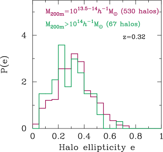
Figure 1: The distribution of halo ellipticity in our simulation. Here we consider two samples: the halos with the mass of $\log(M_{200m}/h^{-1}M_{\odot})=13.5-14$ and $\log(M_{200m}/h^{-1}M_{\odot})>14$.

4.1.1 Halo ellipticity

To examine the dependence of asphericity of halos on the HSSC, we further divide the halo sample into two subsamples with $e\leq\bar{e}$ and $e>\bar{e}$. Here the two-dimensional ellipticity $e$ is defined by $1-q_{2}/q_{1}$ where $q_{1}$ and $q_{2}$ are the major and minor axis lengths, and $\bar{e}$ represents the average ellipticity over the halo sample. We evaluate $q_{1}$ and $q_{2}$ for each halo in the same way as Oguri et al. (2003) by using the three-dimensional information of inertia tensor for each halo. We find $\bar{e}=0.32\pm 0.006$ and $0.29\pm 0.015$ for halo catalogs with $\log(M_{200m}/h^{-1}M_{\odot})=13.5-14$ and $\log(M_{200m}/h^{-1}M_{\odot})\geq 14$, respectively (the uncertainty represents the standard deviation around the mean). For the mass range of $\log(M_{200m}/h^{-1}M_{\odot})=13.5-14$, lower-$e$ and higher-$e$ subsamples have the average ellipticity of $0.21\pm 0.005$ and $0.43\pm 0.006$, respectively. For more massive halos with $\log(M_{200m}/h^{-1}M_{\odot})\geq 14$, the average ellipticities in lower-$e$ and higher-$e$ subsamples are found to be $0.18\pm 0.011$ and $0.40\pm 0.014$. Figure 1 summarizes the distribution of halo ellipticity in our simulated halos.

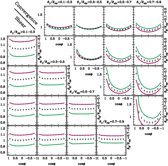
Figure 2: The dependence of the three-point correlation functions on halo ellipticity. We use the halos with the mass of $\log(M_{200m}/h^{-1}M_{\odot})=13.5-14$. The lower-left panels show the HSSC $\zeta_{h++}$ as in Eq. (15), while the upper-right panels show the HKKC, $\zeta_{h\kappa\kappa}$. Note that, in each panel, the three-point correlation function is normalized by the respective two-point correlations. The black points with error bars shows the results for full sample with the average ellipticity of $\bar{e}=0.32$, while the red and green lines are for the subsamples with $\bar{e}=0.21$ and $\bar{e}=0.43$, respectively. The error bars indicate the standard 1-$\sigma$ deviation.

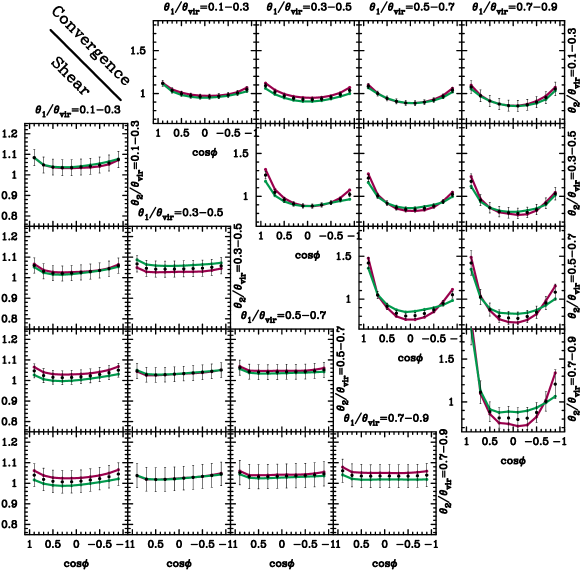
Figure 3: As for Figure 2, but for more massive halos with $\log(M_{200m}/h^{-1}M_{\odot})\geq 14$. The black points with error bars show the results with the average ellipticity of $\bar{e}=0.29$, while the red and green lines are for the subsamples with $\bar{e}=0.18$ and $\bar{e}=0.40$, respectively.

Figures 2 and 3 show the results for the two-halo sample. In each plot, the black points with error bars show the stacked correlations without dividing the sample by halo ellipticity $e$, while the red and green lines are for the subsamples with $e\leq\bar{e}$ and $e>\bar{e}$. In the figures, panels in the lower triangular portion show the correlation of $\zeta_{h++}(\theta_{1},\theta_{2},\phi)$ normalized by $\gamma_{t,0}(\theta_{1})\gamma_{t,0}(\theta_{2})$. The upper triangular portion is for the three-point correlation function in terms of convergence field $\kappa$, $\zeta_{h\kappa\kappa}(\theta_{1},\theta_{2},\phi)$ normalized by $\kappa_{0}(\theta_{1})\kappa_{0}(\theta_{2})$. The black error bars represent the standard deviation of the mean signals. Clearly, the correlation for the lower-mass halos is more sensitive to $e$ (Figure 2). We find that the HKKC at $\theta/\theta_{\rm vir}>0.3$ has a larger amplitude for halos with larger $e$. Furthermore, HKKC tends to show a larger amplitude at $\phi\rightarrow 0$ than $\phi\rightarrow\pi$, because massive subhalos are likely to be detected at outer region of FOF halo. The asymmetry between $\cos\phi=\pm 1$ is also observed in HSSC. We note that the signal at the innermost bin of $\theta$ will be approximated by a simple ellipsoid model presented in Appendix A.

4.1.2 Presence of substructures

We next study how the presence of substructures affects the three-point correlations. In particular, we examine the mass scale of subhalos that give significant contribution, possibly, to HSSC. To this end, we define and use the fractional difference of the three-point correlations as follows:

$$\Delta\zeta(\theta_{1},\theta_{2},\phi;f_{\rm sub,cut})=\frac{\zeta(\theta_{1},\theta_{2},\phi;f_{\rm sub,cut})}{\zeta(\theta_{1},\theta_{2},\phi;{\rm No\,subhalos})}-1,$$ (21)

where $\zeta(\theta_{1},\theta_{2},\phi;{\rm No\,subhalos})$ represents the three-point correlations without substructures and $f_{\rm sub,cut}$ is the threshold as described in Section 3.2. For a given $f_{\rm sub,cut}$, we include only the subhalos whose massese are smaller than $f_{\rm sub,cut}M_{\rm 200m}$.

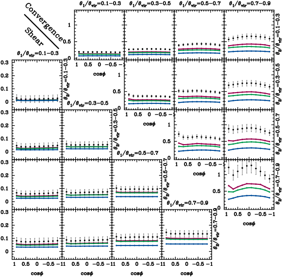
Figure 4: The effect of subhalo abundance on three-point correlation functions. We plot the fractional difference with respect to the result without subhalos (see Eq. [21] for definition). We use halos with $\log(M_{200m}/h^{-1}M_{\odot})=13.5-14$. The black points show the fractional difference between our fiducial case that includes all the subhalos and the result obtained after removing the subhalos. The error bars indicate the standard deviation evaluated in our stacking analysis. Different colored lines represent the results for the projected maps, labeled as SubXXX in Table 1. The red, green and blue correspond to the case of Sub0.10, Sub0.05, and Sub0.01, respectively. Details are found in the text.

Figure 4 shows the result of $\Delta\zeta$ for halos with masses in the range of $\log(M_{200m}/h^{-1}M_{\odot})=13.5-14$. In this figure, the black points show the results with $f_{\rm sub,cut}=1$ (including all the subhalos). The red, green, blue lines represent the result of $f_{\rm sub,cut}=0.1$, 0.05, and 0.01, respectively. The presence of subhalos affects more strongly the HKKC at larger $\theta$, since more massive substructures can survive in high-density regions. On HKKC, the contribution from subhalos with $M_{\rm sub}/M_{200m}\geq 0.1$ can explain a $\sim 50\%$ of amplitude over the wide range of $\theta$. We also find that the presence of substructures increases the overall amplitude of $\zeta$ but does not affect the $\phi$-dependence significantly. A typical difference due to the substructures is found to be $\sim 10\%$ for HSSC and $\sim 100\%$ for HKKC at most. Note that the overall trends in Figure 4 are also found for the halo sample with $\log(M_{200m}/h^{-1}M_{\odot})>14$.

4.2 Projection effect

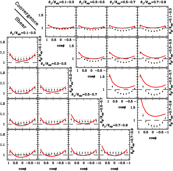
Figure 5: The effect of projected foreground large-scale structure on three-point correlation function. Black points with error bars show the three-point correlation functions for isolated halos. Red lines show the expected correlation signals with projection effects (see also Eq. [22] for detail). We expect that the red line and the black points are close to each other if projection effects are dominated by uncorrelated structure with the target halo. In this figure, we consider the halo sample with $\log(M_{200m}/h^{-1}M_{\odot})=13.5-14$.

So far, we have considered the internal mass distribution of a single halo. In practice, observed lensing signals also contain contribution from the intervening mass distribution along a line of sight. This contamination by uncorrelated large-scale structure is often called a projection effect. It can possibly induce a systematic bias in the correlation analysis. We thus study the projection effect further using our simulations in a direct manner. We generate the projected mass density map by using all the simulations particles in a comoving box with volume of $12.8\times 12.8\times L_{\rm depth}\,(h^{-1}{\rm Mpc})^{3}$, where $L_{\rm depth}$ is the projection depth along the line of sight. We set the projection depth to be $200\,h^{-1}{\rm Mpc}$, the box size of our N-body simulations. Note that we fix the mesh size of comoving $0.025\,h^{-1}{\rm Mpc}$ and the number of meshes ($=512^{2}$) as in Section 3.2.

The projection effect due to uncorrelated structure along a line of sight can be estimated, and hence can be subtracted, by performing the same measurement of the correlation functions around random points. We measure the HSSC and HKKC around random points and construct the following estimator of correlation:

$$\zeta_{\rm est}(\theta_{1},\theta_{2},\phi) = \zeta(\theta_{1},\theta_{2},\phi;{\rm All})-\zeta(\theta_{1},\theta_{2},\phi;{\rm Rand})$$ (22)

$$\,\,\,\,\,\,\,\,\,\,\,\,\,\,\,\,\,\,\,\,\,\,\,\,\,\,\,\,\,\,-\left[\xi(\theta_{1};{\rm All})-\xi(\theta_{1};{\rm Rand})\right]\xi(\theta_{2};{\rm Rand})-\left[\xi(\theta_{2};{\rm All})-\xi(\theta_{2};{\rm Rand})\right]\xi(\theta_{1};{\rm Rand}),$$

where $\zeta({\rm All})$ represents the three-point correlation functions measured including all the simulation particles and with $\zeta({\rm Rand})$ being the measured correlation around random points. Similarly, we define $\xi({\rm All})$ and $\xi({\rm Rand})$ as the two-point correlations around halos and random points, respectively. We have tested and confirmed that the correlation functions around random points converge when the number of random points is set to be ten times as large as the number of halos.

Figure 5 shows the result of $\zeta_{\rm est}$ for the halo catalog with the selection of $\log(M_{200m}/h^{-1}M_{\odot})=13.5-14$. We find that, for HSSC, the signals from the target halos can be recovered after the random contribution is subtracted. On the other hand, the same technique does not work for HKKC. HKKC directly probes the projected mass distribution along a line of sight, and thus the contribution from neighboring (in projection) halos is significant even at small angular scales. The difference between the black points and the red line manifests the projection effect on the HSSC and HKKC; projection of the intervening structure that is physically close to, and hence is correlated with, the lense halo can induce a few percent effects for the HSSC, while it can affect the HKKC by a factor of about $\sim 20\%$. The projection effect is more prominent at large angular scales (large $\theta$), as expected.

4.3 Detectability and implication

In this section, we explore the detectability of HSSC as defined in Eq. (15) and discuss the implication for probing the internal structures of galaxy-group halos and cluster halos.

In the following statistical analysis, we use the HSSC measured with the radial bins of $\theta\,[{\rm arcmin}]=(0.76,2.29)$ and the azimuthal bins of $\cos\phi=(-0.8,-0.4,0,0.4,0.80)$. The bin width of $\theta$ is set to be 16 times $\theta_{\rm mesh}$, where $\theta_{\rm mesh}=0.095\,{\rm arcmin}$ corresponds to the angular size of a mesh in the projected mass map. We use 15 data values of HSSC in total. Note that the binning in radial direction roughly corresponds to $\theta/\theta_{\rm vir}\lower 2.15277pt\hbox{$\;\buildrel<\over{\sim}\;$}0.5$ for the mass-limited sample with $M>10^{14}\,h^{-1}M_{\odot}$ at $z=0.3$. We limit the range of radius as $\theta/\theta_{\rm vir}\lower 2.15277pt\hbox{$\;\buildrel<\over{\sim}\;$}0.5$ because the signals at the outer regions are likely affected by the projection of the neighboring, and hence correlated, structures (see e.g., Figure 5)

4.3.1 Total signal-to-noise ratio

To quantify the detectability of HSSC, we calculate the cumulative signal-to-noise ratio defined as

$$\left(S/N\right)^{2}=\sum_{i,j}\zeta_{h++}(i){\mbox{\boldmath$C$}}^{-1}_{ij}\zeta_{h++}(j),$$ (23)

where indices $i$ and $j$ run over the triangle configurations of interest, $\zeta_{h++}(i)$ denotes the HSSC for the $i$-th triangle configulation, $C$ is the covariance matrix and $C$ is its inverse.

We evaluate the covariance matrix of $C$ on the assumption that the covariance is dominated by the intrinsic ellipticity of sources, the so-called shape noise. We model the shape noise $\epsilon$ by drawing the two-dimensional Gaussian random field on $512^{2}$ mesh points:

$$P(\epsilon)=\frac{1}{\pi\sigma^{2}}\exp\left(-\frac{\epsilon_{1}^{2}+\epsilon_{2}^{2}}{\sigma^{2}}\right),$$ (24)

where $\sigma^{2}=\sigma_{\rm obs}^{2}/n_{\rm gal}\theta_{\rm mesh}^{2}$ with $\theta_{\rm mesh}=0.095$ arcmin, $\sigma_{\rm obs}$ is the rms of observed source ellipticities, and $n_{\rm gal}$ is the number density of sources. In this paper, we assume $\sigma_{\rm obs}=0.4$ and $n_{\rm gal}=30\,{\rm arcmin}^{-2}$, which are expected in a future imaging survey by Large Synoptic Survey Telescope (LSST; LSST Science Collaboration et al., 2009). Note that $\sigma_{\rm obs}$ here includes both galaxy shape noise and measurement uncertainty. Leauthaud et al. (2007) have found that the intrinsic galaxy shape noise was found empirically to be $0.23$ per reduced shear component, while the image simulation for LSST survey indicates that the measurement error in LSST would be of an order of $0.1$ per shear component with r-band limiting magnitude of $\sim 24$ (Bard et al., 2013). Hence, we expect $\sigma_{\rm obs}/\sqrt{2}\sim\sqrt{0.1^{2}+0.23^{2}}=0.25$ per component and this is close to our assumed value of $0.4/\sqrt{2}=0.28$ . We then create 10,000 realizations of noise map and perform the measurements of HSSC in Eq. (15) with respect to the center of map. Using 10,000 HSSCs for the shape noise, we compute the covariance matrix as

$$\bar{\zeta}_{h++,n}(i) = \frac{1}{N_{r}}\sum_{r=1}^{N_{r}}\zeta_{h++,n}(i;r),$$ (25)

$${\mbox{\boldmath$C$}}^{(\rm noise)}_{ij} = \frac{1}{N_{r}-1}\sum_{r=1}^{N_{r}}\left[\zeta_{h++,n}(i;r)-\bar{\zeta}_{h++,n}(i)\right]\left[\zeta_{h++,n}(j;r)-\bar{\zeta}_{h++,n}(j)\right],$$ (26)

where $\zeta_{h++,n}(i;r)$ represents the HSSC for the $i$-th triangle configuration and $r$-th realization of noise map, and $N_{r}=10000$. Since ${\mbox{\boldmath$C$}}^{(\rm noise)}$ corresponds to the statistical uncertainty for individual halos, we derive $C$ by scaling ${\mbox{\boldmath$C$}}^{(\rm noise)}$ with the number of halos $N_{\rm halo}$:

$${\mbox{\boldmath$C$}}=\frac{1}{N_{\rm halo}}{\mbox{\boldmath$C$}}^{(\rm noise)}.$$ (27)

Using Eqs. (23) and (27), we compute the expected $S/N$ for the mass-limited halos at $z=0.33$ as

$$S/N = 1.01\,\sqrt{N_{\rm halo}}\,\,\,\,(M_{200m}\geq 10^{13.5}h^{-1}M_{\odot}),$$ (28)

$$S/N = 2.18\,\sqrt{N_{\rm halo}}\,\,\,\,(M_{200m}\geq 10^{14}h^{-1}M_{\odot}),$$ (29)

where we use the stacked signals for simulated halos in computing of $S/N$. Hence we expect the high-significance measurement of the HSSC using data from future galaxy imaging surveys. We will be able to achieve 5% measurement of HSSCs by using $\sim$400 lenses on galaxy-group scales and $\sim$100 lenses on galaxy-cluster scales.

Table 2: Our model specifications with different properties of the structure of dark matter halos. We perform the subdivision presented in this table for the mass-limited sample with $M_{\rm 200m}\geq 10^{13.5}\,h^{-1}M_{\odot}$ and $10^{14}\,h^{-1}M_{\odot}$.

Model	Halo ellipticity	Subhalo selection	Features
Fiducial	$e=0-1$	All	Our fiducial model with average $e=0.3$
Spherical	$e=0$	None	$\zeta_{h++}(\theta_{1},\theta_{2},\phi)=\xi_{h+}(\theta_{1})\xi_{h+}(\theta_{2})$
Low-$e$	$e=0-0.3$	All	averaged $e=0.2$
Mid-$e$	$e=0.3-0.6$	All	averaged $e=0.4$
High-$e$	$e=0.6-0.9$	All	averaged $e=0.65$
Smooth	$e=0-1$	None	No subhalos
Sub0.05	$e=0-1$	$M_{\rm sub}/M_{200m}<0.05$	Includes only small subhalos
Sub0.10	$e=0-1$	$M_{\rm sub}/M_{200m}<0.10$	Includes massive subhalos

4.3.2 Inferring halo properties

We next examine the ability of the HSSC as a probe of the internal structure of dark matter halos. We define and use the following quantity as a measure of information content:

$$\Delta\chi^{2}=\sum_{ij}\left[\zeta_{h++}(i;{\rm test})-\zeta_{h++}(i;{\rm fid})\right]{\mbox{\boldmath$C$}}_{ij}^{-1}\left[\zeta_{h++}(j;{\rm test})-\zeta_{h++}(j;{\rm fid})\right],$$ (30)

where $\zeta_{h++}(i;{\rm test})$ represents the model HSSC at the $i$-th bin (that we aim at detecting), $\zeta_{h++}(i;{\rm fid})$ is the HSSC of the fiducial model, and $C$ is the covariance defined by Eq. (27). We evaluate the covariance assuming a future imaging survey like LSST. In this section, we define both of $\zeta_{h++}(\rm test)$ and $\zeta_{h++}(\rm fid)$ by using our simulated halos and projected mass density maps. For our fiducial model, we measure the HSSCs for a mass-limited sample with $M_{\rm 200m}\geq M_{\rm thre}$, with two cases of $M_{\rm thre}=10^{13.5}\,h^{-1}M_{\odot}$ and $M_{\rm thre}=10^{14}\,h^{-1}M_{\odot}$. We expect that the former sample corresponds to massive galaxies in Sloan Digital Sky Survey (e.g. Eisenstein et al., 2001), while the latter is for the sample of galaxy clusters identified in optical imaging surveys (e.g. Rykoff et al., 2014).

For a given $M_{\rm thre}$, the simplest reference model assumes spherical halos and no subhalos. Then the expected correlation is expressed as $\zeta_{h++}(\theta_{1},\theta_{2},\phi)=\xi_{h+}(\theta_{1})\xi_{h+}(\theta_{2})$ where $\xi_{h+}$ is defined in Eq (14). Also there is no azimuthal dependence in the correlation. We investigate the sensitivity on halo ellipticity $e$ and the abundance of subhalos. To this end, we divide the mass-limited sample into three subsamples by halo ellipticity or the abundance of subhalos. We use three ellipticity bins: $e=0-0.3,0.3-0.6$, and $0.6-0.9$. Note that we include all the resolved subhalos when calculating the HSSC for these subsamples. Similarly, we consider the dependence of subhalo abundance on the HSSC by using different projected mass maps as in Table 1. We measure the HSSCs by using maps named as “Smooth", “Sub0.05", and “Sub0.10". The first one corresponds to the model in the absence of subhalos, while the last two are for the model including the subhalo with some cutoff of subhalo masses. Table 2 summarizes our subdivision of mass-limited samples.

Table 3: The expected statistical power of the HSSC to constrain the internal structure of dark matter halos. We here present $\Delta\chi^{2}$ defined by Eq. (30). When computing $\Delta\chi^{2}$, we refer the models summarized in Table 2.

$M_{\rm thre}\,[h^{-1}M_{\odot}]$	Spherical	Low-$e$	Mid-$e$	High-$e$	Smooth	Sub0.05	Sub0.10
$10^{13.5}$	$4.14\,(N_{\rm halo}/100)$	$1.72\,(N_{\rm halo}/100)$	$0.816\,(N_{\rm halo}/100)$	$13.6\,(N_{\rm halo}/100)$	$9.83\,(N_{\rm halo}/10^{4})$	$1.78\,(N_{\rm halo}/10^{4})$	$1.21\,(N_{\rm halo}/10^{4})$
$10^{14}$	$25.6\,(N_{\rm halo}/100)$	$0.0938\,(N_{\rm halo}/100)$	$0.251\,(N_{\rm halo}/100)$	$90.7\,(N_{\rm halo}/100)$	$78.7\,(N_{\rm halo}/10^{4})$	$15.4\,(N_{\rm halo}/10^{4})$	$6.01\,(N_{\rm halo}/10^{4})$

We summarize the result of $\Delta\chi^{2}$ for the mass-limited sample with various models of halo ellipticity and subhalo abundance in Table 3. The results in the table are obtained assuming the expected data quality in an LSST-like future imaging survey.

First of all, the HSSC is found to be powerful for examining the simplest model of halo structure as spherical smoothed distribution. For $M_{\rm thre}=10^{14}\,h^{-1}M_{\odot}$, we find $\Delta\chi^{2}\simeq 26$ with 100 halos, showing the spherical halos can be rejected at $\sqrt{26}\simeq 5\sigma$ significance level. Considering massive galaxies with $M_{\rm thre}=10^{13.5}\,h^{-1}M_{\odot}$, we will be able to distinguish between a perfectly spherical and smooth model from our fiducial model at the $5\sigma$ significance level when applying the HSSC analysis to 1000 halos.

Moreover, if we can use 100 halos, we will be able to obtain $\Delta\chi^{2}\simeq 14$ and $90$ for the high-$e$ sample with $M_{\rm thre}=10^{13.5}\,h^{-1}M_{\odot}$ and $M_{\rm thre}=10^{14}\,h^{-1}M_{\odot}$, respectively. Note that the average elliptically $\bar{e}$ is found to be 0.65 for both $M_{\rm thre}$ when we use the high-$e$ sample, while $\bar{e}\simeq 0.3$ is found for our fiducial cases. Hence, using 100 lenses, we can distinguish the model of $\bar{e}\simeq 0.3$ with $\bar{e}=0.65$ with the significance level of $\sqrt{14}\simeq 3.7$ for massive galaxies, while the significance will be $\sqrt{90}\simeq 9.5$ for galaxy clusters. On the other hand, we need a larger number of halos in order to constrain the average halo ellipticity with the level of 0.1. Table 3 shows $\sim 1000$ halos are necessary to detect $3\sigma$ difference between $\bar{e}=0.3$ and $\bar{e}=0.2$ or $0.4$ for $M_{\rm thre}=10^{13.5}\,h^{-1}M_{\odot}$. On the cluster-sized halos, we find the small difference of HSSCs between $\bar{e}=0.3\pm 0.1$, showing much more ($\sim 10,000$) halos are required to improve the constraints of $\bar{e}$. It is worth noting that our definition of $e$ is roughly based on the region within 0.3 times virial radius and the expected constraint of $e$ will depend on its definition.

To infer the abundance of subhalos, we typically require $\sim 10^{4}$ halos to obtain $\Delta\chi^{2}>1$ for either $M_{\rm thre}$. If we consider 10,000 halos with $M_{\rm thre}=10^{13.5}\,h^{-1}M_{\odot}$, we will be able to contain the model in the absence of subhalo with $\sim 3\sigma$ significance, whereas $\sim 10^{5}$ halos are needed to constrain the mass function of subhalos. For the cluster-sized halo, $\sim 1500$ halos are sufficient to reject the model in the absence of subhalo with $\sim 3\sigma$ significance, while we need $\sim 10^{4}$ halos to constrain the subhalo mass function. Therefore, to constrain both of halo ellipticity and subhalo mass function, we require $10^{5}$ objects for massive galaxies and $10^{4}$ objects for clusters. Note that the large number of massive galaxies and clusters are already available in the current galaxy survey (e.g. Anderson et al., 2014; Rykoff et al., 2014), but we need a deeper imaging survey to collect a large number of source galaxies and to measure their shapes.

In the above, we assume that the position of each halo center is precisely known. In real observations, the central position of a cluster-sized halo is assumed to be the position of the brightest cluster galaxy (BCG). Recent observations show that the positions of BCGs are distributed around the the projected halo centers (e.g., Oguri et al., 2010; Zitrin et al., 2012). This off-centering effect has been studied for massive galaxies in Hikage et al. (2013). In the Appendix, we present a simple model of off-centering effect on the three-point correlations. There, we show that the off-centering typically reduces the value of $\Delta\chi^{2}$ in Table 3 by a factor of $\sim 0.5-0.6$. However, the HSSC can still constrain the internal halo structures on a statistical basis.

5 CONCLUSION AND DISCUSSION

We have studied the three-point correlation of the distribution of dark matter halos and the tangential shears of two background sources, referred as to halo-shear-shear correlation (HSSC). We have used the outputs of high-resolution cosmological $N$-body simulations of the standard $\Lambda$CDM model to generate realistic projected density fields around dark halos. Finally, we have studied the information content of HSSCs and quantified the statistical significance of measurement of halo ellipticity and subhalo abundance. Our findings are summarized as follows:

1. HSSC is sensitive to the halo ellipticity $e$ within the virialized region. However, the three-point correlation functions measured for halos in our cosmological simulations are not fully explained by an elliptical halo model. This is because massive subhalos are populated in the outer region of the halo, generating large correlations. HKKC can have an asymmetry between $\phi\rightarrow 0$ and $\phi\rightarrow\pi$ even if all the resolved subhalos are removed. This suggests that even the smooth component of the density field within the halo’s virial radius is different from that of a simple ellipsoid. Halo ellipticity can contribute to the HSSC normalized by its angle average about $\sim 5-10\%$ in the wide range of radii. The sensitivity of the HSSC on $e$ depends on the halo mass.

2. The presence of subhalos can affect the HSSC significantly at larger radii. Subhalos with mass greater than 10% of the host halo mass can give a $\sim 50\%$ contribution to the amplitude of the HKKCs. Also, subhalos do not cause significant azimuthal variation of the three-point correlations. Interestingly, the fractional contribution from subhalos to the HSSC is roughly independent of the host halo mass.

3. We study the detectability of the HSSC assuming the specifics of LSST. When assuming source number density of $30\,{\rm arcmin}^{-2}$, the observed scatter of shape of $0.4$, and source redshift of 1, we expect signal-to-noise (S/N) ratio of the HSSC is $\sim 20$ with $\sim 400$ massive galaxies. A similar S/N can be obtained with $\sim 100$ galaxy clusters. A spherical smoothed mass model can be ruled out with $\sim 5\sigma$ significance level by the HSSC when $100-1000$ halos are observed. For 1000 galaxies with mass greater than $10^{13.5}\,h^{-1}M_{\odot}$, we can distinguish $\bar{e}=0.3$ and $\bar{e}=0.3\pm 0.1$ with a $3\sigma$ significance. On the cluster-sized halos, we need $\sim$10,000 lenses to distinguish $\bar{e}=0.3$ and $\bar{e}=0.3\pm 0.1$ at $3\sigma$ significance. To constrain the mass function of subhalos, we need $\sim 10^{5}$ and $\sim 10^{4}$ halos for massive galaxies and clusters, respectively. Note that observation of such a large number of galaxies and galaxy clusters is indeed possible with the current-generation galaxy surveys (e.g. Anderson et al., 2014; Rykoff et al., 2014), but our proposed statistics require wide and deep imaging data of background galaxies in the future.

Future studies should focus on studying possible systematic effects on the measurement of HSSC. There are likely uncertainties or measurement errors associated with the off-centering effect, the dilution effect by satellite galaxies, the intrinsic alignment of satellite galaxies, and the baryonic effect on the underlying mass distribution (Osato et al., 2015). It is also necessary to develop an accurate theoretical model of the shape and the internal structure of dark matter halos for non-standard dark matter models such as self-interacting dark matter. Future imaging surveys will provide us with rich data that allow us to perform statistical analyses to reveal the nature of dark matter.

Appendix A Toy model

Here we present simple two models of surface mass density at lens plane and use them to derive the three-point correlation of Eq. (15). One assumes the ellipsoid surface mass density and another considers the case of spherical surface mass density in the presence of substructures. Although these simple models will not be suitable for predicting actual HSSC measurements, they are still helpful to understand to what extent the HSSC contains meaningful information of shape and substructures of dark matter halos.

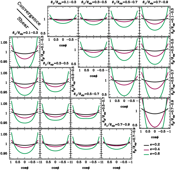
Figure 6: The three-point correlation functions for elliptical NFW halos with $M=10^{14}\,h^{-1}M_{\odot}$, $z=0.3$ and $c_{\rm NFW}=5.6$. Panels in the lower-left portion show the correlation for tangential shear $\zeta_{h++}$ (Eq. [15]), while the upper-right panels show the results for convergence, $\zeta_{h\kappa\kappa}$. Note that the three-point correlation function is normalized by the respective halo-shear or halo-convergence two-point correlations at given $\theta_{1}$ and $\theta_{2}$. The black, red, green, and blue curves in each panel are the results with halo ellipticity $e=0.2$, 0.4, and 0.6, respectively. In each panel, we plot the correlation function measured in the radial bin between $\theta_{1}$ and $\theta_{2}$. The radial coordinate $\theta$ is given in units of the angular virial radius of the halo.

A.1 Elliptical halo

It is well known that the density profile of CDM halos can be approximated as a sequence of the concentric triaxial distribution (e.g. Jing & Suto, 2002). As a reference, we adopt the following mass model:

$$\kappa(\theta,\varphi) = \kappa_{\rm sph}(\vartheta),$$ (31)

$$\vartheta^{2} = \theta^{2}\left[(1-e)^{-1}\cos^{2}\varphi+(1-e)\sin^{2}\varphi\right],$$ (32)

where $\theta$ and $\varphi$ are the radial and azimuthal angles in polar coordinate (the origin is set be the halo centre), $\kappa_{\rm sph}$ represents the radial convergence profile for the spherical NFW profile (e.g. Bartelmann, 1996). The spherical NFW profile can be specified by two parameters, the halo concentration $c_{\rm NFW}$ and mass $M$. Here we define the mass $M=4\pi r^{3}_{\rm vir}\Delta_{\rm vir}(z)\rho_{\rm crit}(z)/3$, where $\rho_{\rm crit}(z)$ is the critical density at cluster redshift $z$, $r_{\rm vir}$ is the virial radius corresponding to the overdensity criterion $\Delta_{\rm vir}(z)$ (as shown in, e.g., Navarro et al. (1997)). In Eq. (31), the halo ellipticity $e$ is defined as $1-q_{2}/q_{1}$ where $q_{1}$ and $q_{2}$ are the major and minor axis lengths of the iso-density contour, respectively. Note that the model of Eq. (31) is consistent with recent observations of galaxy cluster halos (Oguri et al., 2010; Oguri et al., 2012). For the mass model in Eq. (31), we first generate the convergence field in grids, Fourier-transform the convergence field to obtain the Fourier coefficients of the shear field at each grid (see Eqs. (19) and (20)), and then compute the grid-based shear field from the inverse Fourier transform.

Figure 6 shows the HSSC for an elliptical halo. Here we set $M=10^{14}\,h^{-1}M_{\odot}$, $z=0.3$, and $c_{\rm NFW}=5.6$, but vary the halo ellipticity $e$. The lower triangular panels show the correlation of $\zeta_{h++}(\theta_{1},\theta_{2},\phi)$ normalized by $\gamma_{t,0}(\theta_{1})\gamma_{t,0}(\theta_{2})$. Similarly, the upper triangular panels are for the three-point correlation function of $\zeta_{h\kappa\kappa}(\theta_{1},\theta_{2},\phi)$ normalized by $\kappa_{0}(\theta_{1})\kappa_{0}(\theta_{2})$. Figure 6 shows that the normalized three-point functions for an elliptical halo have similar amplitudes at different radii, but stronger azimuthal dependence for larger halo ellipticity. Moreover, the correlation for a squeezed triangle configuration of $\phi\rightarrow 0$ or $\pi$ has larger amplitudes, since the mass density increases along the major axis as in Eq. (31). In general, HSSC shows a smaller azimuthal dependence than HKKC because of the non-local nature of the shear field. In other words, the shear field contains generically information on the surface mass densities over a relatively wide region around the line of sight (e.g., see Eq. [13]). This fact makes it difficult to observe fine features in the local surface mass density with HSSC.

A.2 Spherical halo with substructures

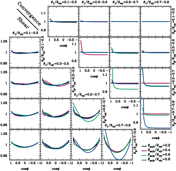
Figure 7: We plot $\zeta_{h++}$ and $\zeta_{h\kappa\kappa}$ as for Figure 6, but with the effect of substructures. Here, we consider a mass model that assumes a spherical NFW main halo with a truncated NFW subhalo. We set the main halo mass to be $M_{\rm host}=10^{14}\,h^{-1}M_{\odot}$, the concentration $c_{\rm NFW,host}=5.6$, and the subshalo mass $M_{\rm sub}=10^{13}\,h^{-1}M_{\odot}$, and the subhalo concentration $c_{\rm sub}=7$. The black, red, green and blue lines in each panel correspond to the model with the subhalo position at $\theta_{\rm sub}/\theta_{\rm vir}=0.2,0.4,0.6$ and 0.8, respectively. We generate 300 realizations for each model, and then calculate the ensemble-averaged three-point functions.

We next consider the presence of substructures in a spherical halo. The standard CDM model predicts that a halo contains abundant substructures (e.g. Tormen et al., 1998; Gao et al., 2004). To examine the effect of substructures in Eqs (15) and (16), we consider the following mass model:

$$\kappa(\theta,\varphi)=\kappa_{\rm sph}(\theta)+\kappa_{\rm sub}(|{\mbox{\boldmath$\theta$}}-{\mbox{\boldmath$\theta$}}_{\rm sub}|),$$ (33)

where we consider the polar coordinate ${\mbox{\boldmath$\theta$}}=(\theta,\varphi)$ and ${\mbox{\boldmath$\theta$}}_{\rm sub}$ located at the center of subhalo with respect to the halo center. In Eq. (33), $\kappa_{\rm sph}$ represents the convergence field for main spherical NFW halo with mass of $M_{\rm host}$ and concentration $c_{\rm NFW,host}$, while $\kappa_{\rm sub}$ expresses the additional contribution from subhalo with mass of $M_{\rm sub}$, concentration $c_{\rm sub}$ and offset radius of $|{\mbox{\boldmath$\theta$}}_{\rm sub}|$. Here we compute $\kappa_{\rm sub}$ by using the mass density profile proposed in Hayashi et al. (2003). Note that our model of $\kappa_{\rm sub}$ includes the truncation of density profile due to tidal stripping (see Section 2.1 in Shirasaki, 2015, for detailed expressions).

To compute the HSSC for the model of Eq. (33), we consider four different subhalo positions, $\theta_{\rm sub}/\theta_{\rm vir}=0.2,0.4,0.6$ and 0.8 and fix the other parameters as follows: $M_{\rm host}=10^{14}\,h^{-1}M_{\odot}$, $c_{\rm NFW,host}=5.6$, $M_{\rm sub}=10^{13}\,h^{-1}M_{\odot}$, $c_{\rm sub}=7$, and the lens redshift of 0.3. For a given set of parameters, we generate 300 independent mass models by randomly setting the azimuthal location of the subhalo, and then compute the shear fields through Fourier transform. We calculate the mean three-point correlations as in Eqs (15) and (16) by averaging over the 300 realizations. Figure 7 shows the model prediction. We find that squeezed triangles with $\phi\rightarrow 0$ give large $\zeta_{h\kappa\kappa}$, while $\zeta_{h\kappa\kappa}$ is small when $\theta_{\rm sub}$ is not in the radial bin between $\theta_{1}$ and $\theta_{2}$. For instance, we find a significant correlation only for $\theta_{1}/\theta_{\rm vir}=\theta_{2}/\theta_{\rm vir}=0.3-0.5$ for $\theta_{\rm sub}/\theta_{\rm vir}=0.4$. This is expected because squeezed triangles with $\theta_{1}\simeq\theta_{2}$ and $\phi\rightarrow 0$ contain lensing signals contributed by the surface mass of substructures. Since our model of $\kappa_{\rm sub}$ predicts a smaller tidal truncation when subhalos are closer to the halo centre, the enhancement in $\zeta_{h\kappa\kappa}$ also becomes smaller at smaller $\theta$ even if the subhalo mass $M_{\rm sub}$ is fixed. The non-local nature of shear field reduce $\zeta_{h++}$ for closed triangles but increase the correlation for more general triangular configurations. Note that the presence of subhalos breaks the azimuthal symmetry in the convergence field, making the angular ($\theta,\varphi$) dependence of the three-point correlation more complicated.

Appendix B Modelling the off-centering effect on halo-shear-shear correlation

In this appendix, we examine the effect of galaxy-halo off-centering on the halo-shear-shear correlation. To perform stacked lensing analyses, it is necessary to determine the central position of the foreground lensing halo. For a galaxy cluster identified in an optical survey, it is often assumed that the brightest cluster galaxy (BCG) is located at the center of its host halo. Recent observations show, however, that BCGs are not always at the center of their host halos, but their positions are distributed with angular offsets from the projected halo centers (e.g., Oguri et al., 2010; Zitrin et al., 2012). Off-centering of massive galaxies have also been studied in Hikage et al. (2013).

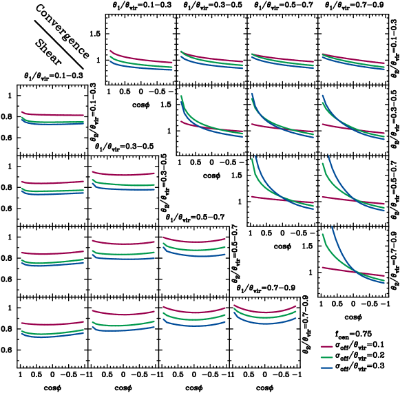
Figure 8: The off-centering effect on the three-point correlations for spherical halos with $M=10^{14}\,h^{-1}M_{\odot}$, $z=0.3$ and $c_{\rm NFW}=5.6$. In this figure, we assume that the off-centering probability is given as in Eq. (34) with $f_{\rm cen}=0.75$. The colored lines show the results with three different off-centering radius, $\sigma_{\rm off}/\theta_{\rm vir}=0.1,0.2$ and 0.3, where $\theta_{\rm vir}$ is the angular virial radius of the halo. The lower triangular panels show the correlation $\zeta_{h++}$, while the upper panels are for $\zeta_{h\kappa\kappa}$. We normalize the three-point correlations by the respective halo-shear or halo-convergence correlation in the absence of off-centering effects. Note that the source redshift is assumed to be 1.

The probability of offset between a reference of halo center and true center in stacked lensing analyses is commonly characterized as

$$p(\theta_{\rm off})=f_{\rm cen}+(1-f_{\rm cen})\frac{\theta_{\rm off}}{\sigma^{2}_{\rm off}}\exp\left(-\frac{\theta^{2}_{\rm off}}{2\sigma^{2}_{\rm off}}\right),$$ (34)

where $\theta_{\rm off}$ represents the offset in angular scale, $f_{\rm cen}$ is the fraction of objects located at true halo center, and $\sigma_{\rm off}$ is the scatter in off-centering probability. To study the impact of possible offsets of the center in stacked analysis, we first consider the simplest case of spherical NFW halos. We generate 300 realizations of spherical NFW halos with mass $M=10^{14}\,h^{-1}M_{\odot}$ and the concentration $c_{\rm NFW}=5.6$ at redshift of 0.3 and then compute projected density in two-dimensional plane assuming the central position of these halos follows the probability as in Eq (34). Using Eqs. (19) and (20), we obtain the corresponding lensing signals for each off-centered halo in two-dimensional image. We then perform stacking analyses of three-point correlation assuming the stacked position is set to be the center of the image.

Figure 8 summarizes the results from stacked analyses of off-centering spherical NFW halos with the source redshift of 1. In this figure, we assume $f_{\rm cen}=0.75$ that is broadly consistent with observations, while varying the scatter of $\sigma_{\rm off}$ as $0.1\theta_{\rm vir}$, $0.2\theta_{\rm vir}$, and $0.3\theta_{\rm vir}$. We find that off-centering effects of a halo-center reference can induce additional correlation signals even if the shape of halo is exactly spherical. The effect on the correlation for convergence can show the significant dependence of azimuthal angle, but it is completely different from the expectation for the elliptical halos (see Figure 6). On the other hand, the off-centering effect can affect the amplitude of halo-shear-shear correlation by a factor of $\sim 0.7$ and the additional azimuthal dependence is found to be relatively small.

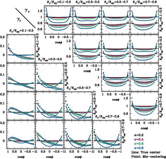
Figure 9: The off-centering effect of three-point correlation for elliptical halos with $M=10^{14}\,h^{-1}M_{\odot}$, $z=0.3$ and $c_{\rm NFW}=5.6$. The upper triangular panels show the correlation for tangential shear $\zeta_{h++}$, while the lower panels show the correlation for cross shear $\zeta_{h\times\times}$. The three-point correlation in each panel is normalized with halo-shear correlation without off-centering effects. In each panel, the colored points represent the case in the presence of off-centering effects, while the lines are for the correlation without off-centering effects. The color differences show the different halo ellipticities of $e=0.2$, 0.4, 0.6, and 0.8. Here we assume $f_{\rm cen}=0.75$ and $\sigma_{\rm off}/\theta_{\rm vir}=0.2$ when including the off-centering effect. Note that the source redshift is assumed to be 1.

Furthermore, we consider the off-centering of elliptical NFW halos as in Eq. (31) assuming $f_{\rm cen}=0.75$ and $\sigma_{\rm off}/\theta_{\rm vir}=0.2$. Similarly to the spherical case, we generate 300 realizations of elliptical NFW halos including the offset of halo positions as in Eq. (34) and derive the lensing quantities through Fourier transformation with Eqs. (19) and (20) in two-dimensional image. We then compute the corresponding stacked lensing signals by setting a reference of halo center to be the center of image. Figure 9 shows the result of our analyses of elliptical NFW halos with possible off-centering effects. The upper triangular panels show the three-point correlation for tangential shear, while the lower panels for cross shear. The lines in this figure correspond to the case of $f_{\rm cen}=1$, while off-centered cases are summarized in the colored points. The difference of colors represents the different halo ellipticities. For the tangential shear, we find that the off-centering effect can mainly change the amplitude of correlation and additional azimuthal dependences will be subdominant. The change of amplitude in $\zeta_{h++}$ can be reasonably approximated as $A_{0}+A_{1}\cos^{2}\phi$, where $A_{0}\simeq 0.6-0.8$ and $A_{1}\sim 0.1$ for $\theta<\theta_{\rm vir}$ and $e\lower 2.15277pt\hbox{$\;\buildrel<\over{\sim}\;$}0.8$. More importantly, the three-point correlation of cross shear is found to be less sensitive to halo ellipticities and they can be used as a proxy of off-centering effects (e.g., see the panel for $\theta_{1}/\theta_{\rm vir}=0.1-0.3$ and $\theta_{2}/\theta_{\rm vir}=0.1-0.3$ in Figure 9).

In a short summary, the off-centering effect of a halo-center reference in stacked analyses can induce additional correlations, but the major effect on $\zeta_{h++}$ can be approximated as the change of amplitude alone. Moreover, the degeneracy between the off-centering effect and underlying correlation induced by halo shapes can be broken when the three-point correlation function for cross shear is properly used. Assuming $f_{\rm cen}=0.75$ and $\sigma_{\rm off}/\theta_{\rm vir}=0.2$, the results in Table 3 will be modified by a factor of $0.7^{2}-0.8^{2}\simeq 0.5-0.6$, while it seems still possible to detect the halo-shear-shear correlation for galaxy clusters and massive galaxies in future imaging surveys.

REFERENCES

- Adhikari et al. (2015) Adhikari S., Chue C. Y. R., Dalal N., 2015, J. Cosmology Astropart. Phys., 1, 009
- Allgood et al. (2006) Allgood B., Flores R. A., Primack J. R., Kravtsov A. V., Wechsler R. H., Faltenbacher A., Bullock J. S., 2006, MNRAS, 367, 1781
- Anderson et al. (2014) Anderson L., et al., 2014, MNRAS, 441, 24
- Applegate et al. (2014) Applegate D. E., et al., 2014, MNRAS, 439, 48
- Bard et al. (2013) Bard D., et al., 2013, ApJ, 774, 49
- Bartelmann (1996) Bartelmann M., 1996, A&A, 313, 697
- Bartelmann & Schneider (2001) Bartelmann M., Schneider P., 2001, Phys.~Rep., 340, 291
- Battaglia et al. (2016) Battaglia N., et al., 2016, J. Cosmology Astropart. Phys., 8, 013
- Brainerd et al. (1996) Brainerd T. G., Blandford R. D., Smail I., 1996, ApJ, 466, 623
- Broadhurst et al. (2005) Broadhurst T., Takada M., Umetsu K., Kong X., Arimoto N., Chiba M., Futamase T., 2005, ApJ, 619, L143
- Chisari et al. (2017) Chisari N. E., et al., 2017, MNRAS, 472, 1163
- Clampitt & Jain (2016) Clampitt J., Jain B., 2016, MNRAS, 457, 4135
- Covone et al. (2014) Covone G., Sereno M., Kilbinger M., Cardone V. F., 2014, ApJ, 784, L25
- Crocce et al. (2006) Crocce M., Pueblas S., Scoccimarro R., 2006, MNRAS, 373, 369
- Dodelson & Widrow (1994) Dodelson S., Widrow L. M., 1994, Physical Review Letters, 72, 17
- Eisenstein et al. (2001) Eisenstein D. J., et al., 2001, AJ, 122, 2267
- Elahi et al. (2014) Elahi P. J., Mahdi H. S., Power C., Lewis G. F., 2014, MNRAS, 444, 2333
- Evans & Bridle (2009) Evans A. K. D., Bridle S., 2009, ApJ, 695, 1446
- Fischer et al. (2000) Fischer P., et al., 2000, AJ, 120, 1198
- Gao et al. (2004) Gao L., White S. D. M., Jenkins A., Stoehr F., Springel V., 2004, MNRAS, 355, 819
- Guzik & Seljak (2002) Guzik J., Seljak U., 2002, MNRAS, 335, 311
- Hayashi et al. (2003) Hayashi E., Navarro J. F., Taylor J. E., Stadel J., Quinn T., 2003, ApJ, 584, 541
- Hikage et al. (2013) Hikage C., Mandelbaum R., Takada M., Spergel D. N., 2013, MNRAS, 435, 2345
- Hoekstra et al. (2004) Hoekstra H., Yee H. K. C., Gladders M. D., 2004, ApJ, 606, 67
- Hoekstra et al. (2012) Hoekstra H., Mahdavi A., Babul A., Bildfell C., 2012, MNRAS, 427, 1298
- Hudson et al. (1998) Hudson M. J., Gwyn S. D. J., Dahle H., Kaiser N., 1998, ApJ, 503, 531
- Jing & Suto (2002) Jing Y. P., Suto Y., 2002, ApJ, 574, 538
- Johnston et al. (2007) Johnston D. E., et al., 2007, preprint, (arXiv:0709.1159)
- Kaiser & Squires (1993) Kaiser N., Squires G., 1993, ApJ, 404, 441
- Kaplinghat et al. (2016) Kaplinghat M., Tulin S., Yu H.-B., 2016, Physical Review Letters, 116, 041302
- Komatsu et al. (2011) Komatsu E., et al., 2011, ApJS, 192, 18
- LSST Science Collaboration et al. (2009) LSST Science Collaboration et al., 2009, preprint, (arXiv:0912.0201)
- Leauthaud et al. (2007) Leauthaud A., et al., 2007, ApJS, 172, 219
- Lewis et al. (2000) Lewis A., Challinor A., Lasenby A., 2000, ApJ, 538, 473
- Mandelbaum et al. (2006a) Mandelbaum R., Seljak U., Kauffmann G., Hirata C. M., Brinkmann J., 2006a, MNRAS, 368, 715
- Mandelbaum et al. (2006b) Mandelbaum R., Hirata C. M., Broderick T., Seljak U., Brinkmann J., 2006b, MNRAS, 370, 1008
- Mandelbaum et al. (2006c) Mandelbaum R., Seljak U., Cool R. J., Blanton M., Hirata C. M., Brinkmann J., 2006c, MNRAS, 372, 758
- Miralda-Escude (1991) Miralda-Escude J., 1991, ApJ, 370, 1
- Navarro et al. (1997) Navarro J. F., Frenk C. S., White S. D. M., 1997, ApJ, 490, 493
- Nishimichi et al. (2009) Nishimichi T., et al., 2009, PASJ, 61, 321
- Oguri et al. (2003) Oguri M., Lee J., Suto Y., 2003, ApJ, 599, 7
- Oguri et al. (2010) Oguri M., Takada M., Okabe N., Smith G. P., 2010, MNRAS, 405, 2215
- Oguri et al. (2012) Oguri M., Bayliss M. B., Dahle H., Sharon K., Gladders M. D., Natarajan P., Hennawi J. F., Koester B. P., 2012, MNRAS, 420, 3213
- Okabe et al. (2013) Okabe N., Smith G. P., Umetsu K., Takada M., Futamase T., 2013, ApJ, 769, L35
- Okumura et al. (2009) Okumura T., Jing Y. P., Li C., 2009, ApJ, 694, 214
- Osato et al. (2015) Osato K., Shirasaki M., Yoshida N., 2015, ApJ, 806, 186
- Parker et al. (2007) Parker L. C., Hoekstra H., Hudson M. J., van Waerbeke L., Mellier Y., 2007, ApJ, 669, 21
- Peter et al. (2013) Peter A. H. G., Rocha M., Bullock J. S., Kaplinghat M., 2013, MNRAS, 430, 105
- Planck Collaboration et al. (2016) Planck Collaboration et al., 2016, A&A, 594, A13
- Rykoff et al. (2014) Rykoff E. S., et al., 2014, ApJ, 785, 104
- Schrabback et al. (2015) Schrabback T., et al., 2015, MNRAS, 454, 1432
- Sheldon et al. (2001) Sheldon E. S., et al., 2001, ApJ, 554, 881
- Shirasaki (2015) Shirasaki M., 2015, ApJ, 799, 188
- Simon et al. (2008) Simon P., Watts P., Schneider P., Hoekstra H., Gladders M. D., Yee H. K. C., Hsieh B. C., Lin H., 2008, A&A, 479, 655
- Simon et al. (2012) Simon P., Schneider P., Kübler D., 2012, A&A, 548, A102
- Simon et al. (2013) Simon P., et al., 2013, MNRAS, 430, 2476
- Spergel & Steinhardt (2000) Spergel D. N., Steinhardt P. J., 2000, Physical Review Letters, 84, 3760
- Springel (2005) Springel V., 2005, MNRAS, 364, 1105
- Springel et al. (2001) Springel V., White S. D. M., Tormen G., Kauffmann G., 2001, MNRAS, 328, 726
- Tegmark et al. (2006) Tegmark M., et al., 2006, Phys. Rev. D, 74, 123507
- Tormen et al. (1998) Tormen G., Diaferio A., Syer D., 1998, MNRAS, 299, 728
- Valageas & Nishimichi (2011) Valageas P., Nishimichi T., 2011, A&A, 527, A87
- Velliscig et al. (2015) Velliscig M., et al., 2015, MNRAS, 453, 721
- Weinberg et al. (2015) Weinberg D. H., Bullock J. S., Governato F., Kuzio de Naray R., Peter A. H. G., 2015, Proceedings of the National Academy of Science, 112, 12249
- White & Hu (2000) White M., Hu W., 2000, ApJ, 537, 1
- Zitrin et al. (2012) Zitrin A., Bartelmann M., Umetsu K., Oguri M., Broadhurst T., 2012, MNRAS, 426, 2944
- van Uitert et al. (2012) van Uitert E., Hoekstra H., Schrabback T., Gilbank D. G., Gladders M. D., Yee H. K. C., 2012, A&A, 545, A71
- van Uitert et al. (2017) van Uitert E., et al., 2017, MNRAS, 467, 4131