Online Strip Packing with Polynomial Migration

Abstract

We consider the relaxed online strip packing problem: Rectangular items arrive online and have to be packed without rotations into a strip of fixed width such that the packing height is minimized. Thereby, repacking of previously packed items is allowed. The amount of repacking is measured by the migration factor, defined as the total size of repacked items divided by the size of the arriving item. First, we show that no algorithm with constant migration factor can produce solutions with asymptotic ratio better than 4/3. Against this background, we allow amortized migration, i. e. to save migration for a later time step. As a main result, we present an AFPTAS with asymptotic ratio $1+\mathcal{O}\left(\epsilon\right)$ for any $\epsilon>0$ and amortized migration factor polynomial in $1/\epsilon$. To our best knowledge, this is the first algorithm for online strip packing considered in a repacking model.

1 Introduction

In the classical strip packing problem we are given a set of two-dimensional items with heights and widths bounded by 1 and a strip of infinite height and width 1. The goal is to find a packing of all items into the strip without rotations such that no items overlap and the height of the packing is minimal. In many practical scenarios the entire input is not known in advance. Therefore, an interesting field of study is the online variant of the problem. Here, items arrive over time and have to be packed immediately without knowing future items. Following the terminology of [11] for the online bin packing problem, in the relaxed online strip packing problem previous items may be repacked when a new item arrives.

There are different ways to measure the amount of repacking in a relaxed online setting. Sanders, Sivadasan, and Skutella introduced the migration model in [24] for online job scheduling on identical parallel machines as follows: When a new job of size $p_{j}$ arrives, jobs of total size $\mu p_{j}$ can be reassigned, where $\mu$ is called the migration factor. In the context of online strip packing the migration factor $\mu$ ensures that the total area of repacked items is at most $\mu$ times the area of the arrived item. We call this the strict migration model.

By a well known relation between strip packing and parallel job scheduling [15], any (online) strip packing algorithm applies to (online) scheduling of parallel jobs. The latter problem is highly relevant e. g. in computer systems [15, 27, 23].

Preliminaries

Since strip packing is NP-hard [1], research focuses on efficient approximation algorithms. Let $A(I)$ denote the packing height of algorithm $A$ on input $I$ and $\operatorname{OPT}(I)$ the minimum packing height. The absolute (approximation) ratio is defined as $\sup_{I}A(I)/\operatorname{OPT}(I)$ while the asymptotic (approximation) ratio as $\lim\sup_{\operatorname{OPT}(I)\rightarrow\infty}\allowbreak A(I)/\operatorname{OPT}(I)$. A family of algorithms $\{A_{\epsilon}\}_{\epsilon>0}$ is called polynomial-time approximation scheme (PTAS), when $A_{\epsilon}$ runs in polynomial-time in the input length and has absolute ratio $1+\epsilon$. If the running time is also polynomial in $1/\epsilon$, we call $\{A_{\epsilon}\}_{\epsilon>0}$ fully polynomial-time approximation scheme (FPTAS). Similarly, the terms APTAS and AFPTAS are defined using the asymptotic ratio.

All ratios of online algorithms in the following are competitive, i. e. online algorithms are compared with an optimal offline algorithm.

1.1 Related Work

Offline

Strip packing is one of the classical packing problems and receives ongoing research interest in the field of combinatorial optimization. Since Baker, Coffman and Rivest [1] gave the first algorithm with asymptotic ratio 3, strip packing was investigated in many studies, considering both asymptotic and absolute approximation ratios. We refer the reader to [6] for a survey. A well-known result is the AFPTAS by Kenyon and Rémila [21]. Concerning the absolute ratio, currently the best known algorithm of ratio $5/3+\epsilon$ for any $\epsilon>0$ is by Harren et al.[14].

An interesting result was given by Han et al.in 2007. In [13], they studied the relation between bin packing and strip packing and developed a framework between both problems. For the offline case it is shown that any bin packing algorithm can be applied to strip packing while maintaining the same asymptotic ratio.

Online

The first algorithm for online strip packing was given by Baker and Schwarz [2] in 1983. Using the concept of shelf algorithms [1], they derived the algorithm First-Fit-Shelf with asymptotic ratio arbitrary close to $1.7$ and absolute ratio 6.99 (where all rectangles have height at most $h_{\max}~{}=~{}1$). Later, Csirik and Woeginger [8] showed a lower bound of $h_{\infty}\approx 1.69$ on the asymptotic ratio of shelf algorithms and gave an improved shelf algorithm with asymptotic ratio $h_{\infty}+\epsilon$ for any $\epsilon>0$.

The framework of Han et al.[13] is applicable in the online setting if the online bin packing algorithm belongs to the class Super Harmonic. Thus, Seiden’s online bin packing algorithm Harmonic++ [25] implies an algorithm for online strip packing with asymptotic ratio 1.58889. In 2007 and 2009, the concept of First-Fit-Shelf by Baker and Schwarz was improved independently by two research groups, Hurink and Paulus [15] and Ye, Han, and Zhang [28]. Both improve the absolute competitive ratio of from 6.99 to 6.6623 without a restriction on $h_{\max}$. Further results on special variants of online strip packing were given by Imeh [17] and Ye, Han, and Zhang [29].

On the negative side, there is no algorithm for online strip packing (without repacking) with an asymptotic ratio better then 1.5404 since the lower bound in [3] for online bin packing is also valid for online strip packing. Regarding the absolute ratio, the first lower bound of 2 from [5] was improved in several studies [19, 16, 22]. Currently, the best known lower bound by Yu, Mao, and Xiao [30] is $(3+\sqrt{2})/2\approx 2.618$.

Related results on the migration model

Since its introduction by Sanders, Sivadasan, and Skutella [24], the migration model became increasingly popular. In the context of online scheduling on identical machines, Sanders, Sivadasan, and Skutella [24] gave a PTAS with migration factor $2^{\mathcal{O}\left((1/\epsilon)\log^{2}(1/\epsilon)\right)}$ for the objective of minimizing the makespan. Thereby, the migration factor in [24] depends only on the approximation ratio $\epsilon$ and not on the input size. Such algorithms are called robust.

Skutella and Verschae [26] studied scheduling on identical machines while maximizing the minimum machine load, called machine covering. They considered the fully dynamic setting in which jobs are also allowed to depart. Skutella and Verschae showed that there is no PTAS for this problem in the migration model, which is due to the presence of very small jobs. Instead, they introduced the reassignment cost model, in which the migration factor is defined amortized. Using the reassignment cost model, they gave a robust PTAS for the problem with amortized migration factor $2^{\mathcal{O}\left((1/\epsilon)\log^{2}(1/\epsilon)\right)}$.

Also online bin packing has been investigated in the migration model in a sequence of papers, inspired by the work of Sanders, Sivadasan, and Skutella [24]: The first robust APTAS for relaxed online bin packing was given in 2009 by Epstein and Levin [10]. They obtained an exponential migration factor $2^{\mathcal{O}\left((1/\epsilon^{2})\log 1/\epsilon\right)}$. In 2013, Jansen and Klein [18] improved this result and gave an AFPTAS with polynomial migration factor $\mathcal{O}\left(\frac{1}{\epsilon^{3}}\log\frac{1}{\epsilon^{4}}\right)$. The development of advanced LP/ILP-techniques made this notable improvement possible. Furthermore, in [4] Berndt, Jansen, and Klein built upon the techniques developed in [18] to give an AFPTAS for fully dynamic bin packing with a similar migration factor.

Recently, Gupta et al.[12] studied fully dynamic bin packing with several repacking measures. In the amortized migration model, they presented an APTAS with amortized migration factor $\mathcal{O}\left(1/\epsilon\right)$. Further, this is shown to be optimal by providing a lower bound of of $\Omega(1/\epsilon)$ for any such algorithm in the amortized migration model.

Our contribution

To the authors knowledge, there exists currently no algorithm for online strip packing in the migration or any other repacking model. Therefore, we present novel ideas to obtain the following results: First, a relatively simple argument shows that in the strict migration model it is not possible to maintain solutions that are close to optimal. We prove the following theorem in Section 1.3:

Theorem 1.1.

In the strict migration model, there is no approximation algorithm for relaxed online strip packing with asymptotic competitive ratio better than $4/3$.

Therefore, it is natural to relax the strict migration model such that amortization is allowed in order to obtain an asymptotic approximation scheme. We say that an algorithm has an amortized migration factor of $\mu$ if for every time step $t$ the total migration (i. e. the total area of repacked items) up to time $t$ is bounded by $\mu\sum_{j=1}^{t}\operatorname{SIZE}(i_{j})$, where $\operatorname{SIZE}(i_{j})$ is the area of item $i_{j}$ arrived at time $j$. Adapted to scheduling problems this corresponds with the reassignment cost model introduced by Skutella and Verschae in [26]. We adapt several offline and online techniques and combine them with our novel approaches to obtain the following main result:

Theorem 1.2.

There is a robust AFPTAS for relaxed online strip packing with an amortized migration factor polynomial in $1/\epsilon$.

1.2 Technical Contribution

A general approach in the design of robust online algorithms is to rethink existing algorithmic strategies that work for the corresponding offline problem in a way that the algorithm can adapt to a changing problem instance. The experiences that were made so far in the design of robust algorithms (see [18, 4, 26]) are to design the algorithm in a way such that the generated solutions fulfill very tight structural properties. Such solutions can then be adapted more easily as new items arrive.

A first approach would certainly be do adapt the well known algorithm for (offline) strip packing by Kenyon and Rémila [21] to the online setting. However, we can argue that the solutions generated by this algorithm do not fulfill sufficient structural properties. In the algorithm by Kenyon and Rémila, the strip is divided vertically into segments, where each segment is configured with a set of items. Thereby, each segment can have a different height. Now consider the online setting, where we are asked for a packing for the enhanced instance that maintains most parts of the existing packing. Obviously, it is not enough to place new items on top of the packing as this would exceed the approximation guarantee. Instead, existing configurations of the segments need to be changed to guarantee a good competitive ratio. However, this seems to be hard to do as the height of a configuration can change. Gaps can occur in the packing as a segment might decrease in height or vice versa a segment might increase in height and therefore does not fit anymore in its current position. Over time this can lead to a very fragmented packing. On the other hand, closing gaps in a fragmented packing can cause a huge amount of repacking.

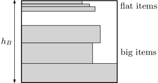
(a) Packing of items in a container

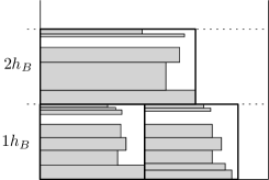
(b) Packing of containers in the strip

Figure 1: Packing structure of our approach. Items are packed into containers of fixed height $h_{B}$, thus the packing of containers results in a bin packing problem.

Containers

In order to maintain packings with a more modular structure, items are batched to larger rectangles of fixed height, called containers (see Figure 1(a)). The width of a container equals the width of the widest item inside. As each container has the same height $h_{B}$, the strip is divided into levels of equal height $h_{B}$ (see Figure 1(b)) and the goal is to fill each level with containers best possible. Thus, finding a container packing is in fact a bin packing problem, where levels correspond with bins and the sizes of the bin packing items are given by the container widths. This approach was studied in the offline setting by Han et al.in [13], while an analysis in a migration setting is more sophisticated.

Thus, the packing of items into the strip is given by two assignments: By the container assignment each item is assigned to a container. Moreover, the level assignment describes which container is placed in which level (corresponds with the bin packing solution). To guarantee solutions with good approximation ratio, both functions have to satisfy certain properties.

Dynamic rounding / Invariant properties

For the container assignment, a natural choice would be to assign the widest items to the first container, the second widest to the second container, and so on [13]. However, in the online setting we can not maintain this strict order while bounding the repacking size. Therefore, we use a relaxed ordering by introducing groups for containers of similar width and requiring the sorting over the groups, rather than over containers. For this purpose, we adapt the dynamic rounding technique developed by Berndt, Jansen, and Klein in [4] to state important invariant properties.

Shift

In order to insert new items, we develop an operation called Shift. The idea is to move items between containers of different groups such that the invariant properties stay fulfilled. When inserting an item $i_{t}$ via Shift into group $g$, items are moved from $g$ to the group $\mathit{left}(g)$, where again items are shifted to the next group, and so on (see Figure 2). Thereby, the total height of the shifted items can increase in each step. However, it is limited such that items that can not be shifted further (at group $g_{0}$ in Figure 2) can be packed into one additional container. This way, we get a new container assignment for the enhanced instance which maintains the approximation guarantee and all desired structural properties.

LP/ILP-techniques

As a consequence of the shift operation, a new container may has to be inserted into the packing. We apply the LP/ILP-techniques developed in [18] to maintain a good level assignment while keeping the migration factor polynomial in $1/\epsilon$.

Packing of small items

Another challenging part regards the handling of items with small area. Without maintaining an advanced structure, small items can fractionate the packing in a difficult way. Such difficulties also arise in related optimization problems, see e.g. [26, 4]. For the case of flat items (small height) we overcome these difficulties by the packing structure shown in Figure 1(a): Flat items are separated from big items in the containers and are sorted by width such that the least wide item is at the top. Narrow items (small width) can be used to fill gaps in the packing when they are grouped to similar height.

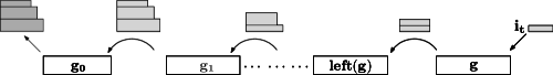
Figure 2: Shift operation moves widest items between groups to insert new item $i_{t}$.

1.3 Lower Bound

In this section we prove Theorem 1.1. We use an adversary to construct an instance $I$ with arbitrary optimal packing height, but $A(I)\geq\frac{4}{3}\operatorname{OPT}(I)$ for any such algorithm $A$.

Proof. Let $A$ be an algorithm for relaxed online strip packing with migration factor $\mu$. We show that for any height $h$ there is an instance $I$ with $\operatorname{OPT}(I)\geq h$ and $A(I)\geq\frac{4}{3}\operatorname{OPT}(I)$. The instance consists of two item types:

A big item has width $\frac{1}{2}-\epsilon$ and height $1$, while a flat item has width $\frac{1}{2}+\epsilon$ and height $\frac{1}{2\left\lceil{\mu}\right\rceil}$ for $\epsilon<1/6$. Note that $A$ can not repack a big item $b$ when a flat item $f$ arrives, as $\operatorname{SIZE}(b)>\mu\operatorname{SIZE}(f)$.

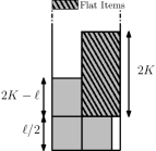
Figure 3: Optimal online packing

First, the adversary sends $2K$ big items, where $K=3\left\lceil{h}\right\rceil$. Let $\ell$ be the number of big items that are packed by $A$ next to another big item. The packing has a height of at least $\frac{\ell}{2}+2K-\ell=2K-\frac{\ell}{2}$ (see Figure 3). Since the optimum packing height for $2K$ big items is $K$, algorithm $A$ has an absolute ratio of at least $2-\frac{\ell}{2K}$. If $\ell\leq\frac{4K}{3}$, the absolute ratio is at least $\frac{4}{3}$ and nothing else is to show.

Now assume $\ell>\frac{4K}{3}$. In this case, the adversary sends $k=4\left\lceil{\mu}\right\rceil K$ flat items of total height $2K$. In the optimal packing of height $2K$ big items and flat items form separate stacks placed in parallel. Note that no two flat items can be packed in parallel. Since $A$ can not repack any big item when a flat item arrives, in the best possible packing achievable by $A$ flat items of total height $2K-\ell$ are packed next to big items (see Figure 3, flat items are packed in the dashed area). Therefore, the packing height is at least $2K+\frac{\ell}{2}$ and hence the absolute ratio is at least $1+\frac{\ell}{4K}\geq\frac{4}{3}$.

In either case, it follows that the asymptotic ratio is at least $4/3$ by considering $h\to\infty$.

1.4 Remainder of the paper

The following section introduces the approach of packing items into containers. We formulate central invariant properties and prove important consequences of this approach. Section 3 presents operations that change the packing in the online setting while maintaining the invariant properties. Up to that section, items of small width were omitted. In Section 4 we show how to integrate them into the container packing. Finally, in Section 5 the amount of migration is analyzed.

Throughout the following sections, let $\epsilon\in(0,1/4]$ be a constant such that $1/\epsilon$ is integer. We denote the height and width of an item $i$ by $h(i)$ and $w(i)$ (both at most 1) and define $\operatorname{SIZE}(i)=w(i)h(i)$. An item $i$ is called big if $h(i)\geq\epsilon$ and $w(i)\geq\epsilon$, flat if $w(i)\geq\epsilon$ and $h(i)<\epsilon$, and narrow if $w(i)<\epsilon$. Accordingly, we partition the instance $I$ into $I_{L}$, the set of big and flat items (having minimum width $\epsilon$), and $I_{N}$, the set of narrow items. If $R$ is a set of items, let $\operatorname{SIZE}(R)=\sum_{i\in R}\operatorname{SIZE}(i)$ and $h(R)=\sum_{i\in R}h(i)$.

2 Container Packing

Let $h_{B}\geq 1$ be the height of a container and let $\mathcal{C}$ denote the set of containers. In the following sequence of definitions we describe the container-packing approach formally. In the first definition, a container $c\in\mathcal{C}$ is an object without geometric interpretation to which items from $I_{L}$ can be assigned to, while satisfying the height capacity:

Definition 2.1 (Container assignment).

A function $\mathit{con}\colon I_{L}\rightarrow\mathcal{C}$ is called a container assignment if $\sum_{i\colon\mathit{con}(i)=c}h(i)\leq h_{B}$ holds for each $c\in\mathcal{C}$.

The next definition shows how to build the container instance, i. e. the strip packing instance which allows to pack $I_{L}$ according to a container assignment.

Definition 2.2 (Container instance).

Let $\mathit{con}\colon I_{L}\rightarrow\mathcal{C}$ be a container assignment. The container instance to $\mathit{con}$, denoted by $C_{\mathit{con}}$, is the strip packing instance defined as follows: For each $c\in\mathcal{C}$ such that there is an $i\in I_{L}$ with $\mathit{con}(i)=c$, define a rectangle $\bar{c}\in C_{\mathit{con}}$ of fixed height $h(\bar{c})=h_{B}$ and width $w(\bar{c})=\max_{i\in I_{L}}\{w(i)\mid\mathit{con}(i)=c\}$.

Since by Definition 2.2 each container $c\in\mathcal{C}$ corresponds with a unique rectangle $\bar{c}\in C_{\mathit{con}}$, in the following we use both notions synonymously.

Like shown in Figure 1(a), big and flat items are placed inside the container differently:

• Big items form a stack starting from the bottom.

• Flat items form a stack starting from the top. Thereby, items in that stack are sorted such that the least wide item is placed at the top edge of the container.

The need for the special structure for flat items will become clear in Section 3.5.3.

In order to solve the container packing problem via a linear program (LP), the number of occurring widths has to be bounded. For this purpose we define a rounding function $R\colon\mathcal{C}\rightarrow G$ that maps containers to groups. The concrete rounding function will be specified later. Using $R$ we obtain the rounded container instance by rounding up each container to the widest in its group.

Definition 2.3 (Rounded container instance).

Let $C_{\mathit{con}}$ be a container instance and $R\colon\mathcal{C}\rightarrow G$ be a rounding function. The rounded container instance $C_{\mathit{con}}^{R}$ is obtained from the container instance $C_{\mathit{con}}$ by setting the width of each container $c$ to a new width $w^{R}(c)\geq w(c)$ with $w^{R}(c):=\max_{c^{\prime}\in\mathcal{C}}\{w(c^{\prime})\mid R(c^{\prime})=R(c)\}$.

2.1 LP Formulation

By Definition 2.3 a rounded container instance has only containers of $\left|{G}\right|$ different widths. Therefore we can use the following LP formulation to find a level assignment. It is commonly used for bin packing problems and was first described by Eisemann [9].

Definition 2.4 (LP($C$)).

Let $C$ be a container instance and assume that items from $C$ have one of $m$ different widths $w_{1},\ldots,w_{m}\geq\epsilon$. Let $P$ be the set of patterns and $n=\left|{P}\right|$. A pattern $P_{i}\in P$ is a multiset of widths $\{a(P_{i},1):n_{1},a(P_{i},2):n_{2},\ldots a(P_{i},m):n_{M}\}$ where $a(P_{i},j)$ for $1\leq i\leq n$ and $1\leq j\leq m$ denotes how often width $w_{j}$ appears in pattern $P_{i}$. Let $b_{j}$ for $1\leq j\leq m$ be the number of containers having width $w_{j}$. LP($C$) is defined as:

$$\min \left\lVert x\right\rVert_{1}$$

s.t. $$\sum_{P_{i}\in P}x_{i}a(P_{i},j)\geq b_{j} \forall 1\leq j\leq m$$

$$x_{i}\geq 0 \forall 1\leq i\leq n$$

The value $\left\lVert x\right\rVert_{1}$ of an optimal solution to the above LP relaxation is denoted by $\operatorname{LIN}(C)$. If $y\in\mathbb{N}^{n}$ is an optimal solution to the LP with integer constraints $x_{i}\in\mathbb{Z}^{+}$, its value is denoted with $\operatorname{OPT}(C)$. Note that $\operatorname{LIN}(C)\leq\operatorname{OPT}(C)$.

Since all containers have width greater or equal $\epsilon$, each level has at most $1/\epsilon$ slots. In each slot, there are $m+1$ possibilities to fill the slot: Either one container of the $m$ different sizes is placed there, or the slot stays empty. Therefore, $n\leq(m+1)^{1/\epsilon}$.

2.2 Grouping

In the next subsection we adapt the dynamic rounding technique developed in [4] for containers. It is based on the one by Karmarkar and Karp [20] for (offline) bin packing, but modified for a dynamic setting.

2.2.1 Basic Definitions

Each container is assigned to a (width) category $l\in\mathbb{N}$, where container $c$ has width category $l$ if $w(c)\in(2^{-(l+1)},2^{-l}]$. Let $W$ denote the set of all non-empty categories, i. e. $W=\{l\in\mathbb{N}\mid\exists c\in\mathcal{C}~{}w(c)\in(2^{-(l+1)},2^{-l}]\}$.

Lemma 2.5.

The set $W$ of categories has at most $\omega:=\left\lfloor{\log\frac{1}{\epsilon}}\right\rfloor+1$ elements.

Proof.

Containers can have any width between $\epsilon$ and 1, just like the width of big and flat items. The widest containers belong to category 0, while containers of minimum width $\epsilon$ are assigned to the category $\left\lfloor{\log\frac{1}{\epsilon}}\right\rfloor$. Thus $\left|{W}\right|\leq\omega$. ∎

Figure 4: Groups of one category $l\in W$ and number of containers $K_{g}$ per group

Furthermore, we build groups within the categories: A group $g\in G$ is a triple $(l,X,r)$, where $l\in W$ is the category, $X\in\{A,B\}$ is the block, and $r\in\mathbb{N}$ is the position in the block. The maximum position of category $l$ at block $X$ that is non-empty is denoted by $q(l,X)$. Figure 4 outlines the groups and the block structure of one category $l\in W$ (the values for $K_{g}$ will become clear in Section 2.2.2).

By the notion of blocks, groups of one category can be partitioned into two types. This becomes helpful to maintain the invariant properties with respect to the growing set of items. More details on that are given in the later Sections 2.2.2 and 3.5.2. For a group $g=(l,X,r)$ we define the group to the left of it as follows:

$$\mathit{left}(g)=\begin{cases}(l,X,r-1)&\mbox{if }r>0\vee X=A\\ (l,A,q(l,A))&\mbox{if }r=0\wedge X=B\\ \end{cases}$$

Analogously, we say $g=\mathit{right}(g^{\prime})$, if $\mathit{left}(g)=g^{\prime}$ holds. We set $\mathit{left}((l,A,0))=(l,A,-1)$ and $\mathit{right}((l,B,q(l,B)))=(l,B,q(l,B)+1)$ as empty groups.

From now on, let a rounding function $R$ and a container assignment $\mathit{con}$ be given. Let $K_{g}=\left|{\{c\in\mathcal{C}\mid R(c)=g\}}\right|$ be the number of containers of group $g$. We say that item $i$ has group $g$ if $R(\mathit{con}(i))=g$, that is, item $i$ is in a container which belongs to group $g$. Let ${I_{L}}^{g}=\{i\in I_{L}\mid R(\mathit{con}(i))=g\}$ be the set of items of group $g$ and define $h(g)=\sum_{i\in{I_{L}}^{g}}h(i)$ as the total height of those items.

2.2.2 Invariant Properties

In Section 1.2 we argued that only solutions with strong structural properties can be adapted appropriately in the online setting while maintaining a good competitive ratio. In Definition 2.6 we state a set of invariant properties, to which we refer with ($\mathcal{I}$1)-($\mathcal{I}$5) in the remainder of this paper.

Definition 2.6 (Invariant properties).

Let $k\in\mathbb{N}$ be a parameter.

1. Width categories
   $2^{-(l+1)}<w(i)\leq 2^{-l}$        for all $i\in{I_{L}}^{g}$ s.t. $g=(l,\cdot,\cdot)$

2. Sorting of items over groups
   $w(i)\geq w(i^{\prime})$        for all $i\in{I_{L}}^{g},i^{\prime}\in{I_{L}}^{g^{\prime}}$ s.t. $g=\mathit{left}(g^{\prime})$

3. Number of containers in block A
   $K_{(l,A,0)}\leq 2^{l}k$,
   $K_{(l,A,r)}=2^{l}k$        for all $l\in W$ and $1\leq r\leq q(l,A)$

4. Number of containers in block B
   $K_{(l,B,q(l,B))}\leq 2^{l}(k-1)$,
   $K_{(l,B,r)}=2^{l}(k-1)$        for all $l\in W$ and $0\leq r<q(l,B)$

5. Total height of items per group
   $(h_{B}-1)(K_{g}-1)\leq h(g)\leq(h_{B}-1)K_{g}$        for all $g\in G$

Property ($\mathcal{I}$1) ensures that each item is assigned to the right category. Note that as a consequence, each container of a group $(l,\cdot,\cdot)$ has a width in $(2^{-(l+1)},2^{-l}]$. By property ($\mathcal{I}$2), all items in a group $g$ have a width greater or equal than items in the group $\mathit{right}(g)$. That is, instead of a strict order over all containers, ($\mathcal{I}$2) ensures an order over groups of containers. The properties ($\mathcal{I}$3) and ($\mathcal{I}$4) set the number of containers to a fixed value, except for special cases (see Figure 4): Groups in block $A$ have more containers than groups in block $B$. Moreover, there are two flexible groups (namely $(l,A,0)$ and $(l,B,q(l,B))$) whose number of containers is only upper bounded. Finally, property ($\mathcal{I}$5) ensures an important relation between items and containers of a group $g$: Since $h(g)\leq K_{g}(h_{B}-1)$, at least one of the $K_{g}$ containers has a filling height of at most $h_{B}-1$ and thus can admit a new item. However, the lower bound $(h_{B}-1)(K_{g}-1)\leq h(g)$ ensures that each container is well filled in an average container assignment.

2.2.3 Number of Groups

One of the important consequences of the invariant properties is the fact that the number of non-empty groups $\left|{G}\right|$ can be bounded from above, assuming that the instance is not too small. Therefore, the parameter $k$ has to be set in a particular way:

Lemma 2.7.

Let $\omega$ be defined like in Lemma 2.5. For $k=\left\lfloor{\frac{\epsilon}{4\omega h_{B}}\operatorname{SIZE}(I_{L})}\right\rfloor$ the number of non-empty groups in $G$ is bounded by $\mathcal{O}\left(\frac{\omega}{\epsilon}\right)$, assuming that $\operatorname{SIZE}(I_{L})\geq\frac{24\omega h_{B}(h_{B}-1)}{\epsilon h_{B}-2\epsilon}$.

Proof.

Let $G_{1}=G\setminus\left(\bigcup_{l\in W}(l,A,0)\cup\bigcup_{l\in W}(l,B,q(l,B))\right)$ and let $g\in G_{1}$. Since by property ($\mathcal{I}$1) every container of group $g$ has width greater than $2^{-(l+1)}$, it follows together with the further invariant properties

$$\operatorname{SIZE}({I_{L}}^{g}) >2^{-(l+1)}(h_{B}-1)(K_{g}-1) \mathcal{I} \mathcal{I}$$ (1), (5)

$$\geq 2^{-(l+1)}(h_{B}-1)(2^{l}(k-1)-1) \mathcal{I} \mathcal{I}$$ (3), (4)

$$=\frac{1}{2}(h_{B}-1)(k-1)-2^{-(l+1)}(h_{B}-1)$$

$$\geq\frac{1}{2}(h_{B}-1)(k-1)-\frac{h_{B}-1}{2}$$

$$=\frac{1}{2}(h_{B}-1)(k-2)\,.$$

Now, let $I_{L}^{(l)}$ be the set of items in $I_{L}$ which belong to containers of category $l$. It holds that $\operatorname{SIZE}(I_{L}^{(l)})\geq\sum_{g=(l,\cdot,\cdot)\in G_{1}}\operatorname{SIZE}({I_{L}}^{g})\geq(q(l,A)+q(l,B))\left(\frac{1}{2}(h_{B}-1)(k-2)\right)$ and resolving leads to

$$q(l,A)+q(l,B)\leq\frac{2\operatorname{SIZE}(I_{L}^{(l)})}{(h_{B}-1)(k-2)}\,.$$ (2.1)

We now show $(h_{B}-1)(k-2)\geq\frac{\epsilon}{8\omega h_{B}}\operatorname{SIZE}(I_{L})$. The assumption on $\operatorname{SIZE}(I_{L})$ is equivalent to $\frac{\epsilon}{4\omega h_{B}}\operatorname{SIZE}(I_{L})-3\geq\frac{\epsilon}{8\omega(h_{B}-1)}\operatorname{SIZE}(I_{L})$. Therefore,

$$k-2=\left\lfloor{\frac{\epsilon}{4\omega h_{B}}\operatorname{SIZE}(I_{L})}\right\rfloor-2\geq\frac{\epsilon}{4\omega h_{B}}\operatorname{SIZE}(I_{L})-3\geq\frac{\epsilon}{8\omega(h_{B}-1)}\operatorname{SIZE}(I_{L})$$

and thus

$$(h_{B}-1)(k-2)\geq\frac{(h_{B}-1)\epsilon}{8\omega(h_{B}-1)}\operatorname{SIZE}(I_{L})=\frac{\epsilon}{8\omega}\operatorname{SIZE}(I_{L})\,.$$

Further, we get

$$\frac{2\operatorname{SIZE}(I_{L})}{(h_{B}-1)(k-2)}\leq\frac{2\operatorname{SIZE}(I_{L})}{\frac{\epsilon}{8\omega}\operatorname{SIZE}(I_{L})}=\frac{16\omega}{\epsilon}\,.$$ (2.2)

As shown in Figure 4, for each category $l$ there are $q(l,A)+q(l,B)+2$ groups. Now, summing over all categories $l\in W$ concludes the proof:

$$~{}~{}~{}\sum_{l\in W}q(l,A)+q(l,B)+2$$

$$\leq\sum_{l\in W}\left(\frac{2\operatorname{SIZE}({I_{L}^{(l)})}}{(h_{B}-1)(k-2)}+2\right)$$ eq. (2.1)

$$=2\left|{W}\right|+\frac{2}{(h_{B}-1)(k-2)}\sum_{l\in W}\operatorname{SIZE}(I_{L}^{(l)})$$

$$=2\left|{W}\right|+\frac{2\operatorname{SIZE}(I_{L})}{(h_{B}-1)(k-2)}$$

$$\leq 2\omega+\frac{16\omega}{\epsilon}$$ eq. (2.2)

∎

2.3 Approximation Guarantee

If the invariant properties of Definition 2.6 are fulfilled, the rounded container instance yields a good approximation to $I_{L}$. Using a proof technique from [13] we are able to prove the following theorem.

Theorem 2.8.

Let $\mathit{con}\colon I_{L}\rightarrow\mathcal{C}$ be a container assignment and $R\colon\mathcal{C}\rightarrow G$ be a rounding function such that invariant properties ($\mathcal{I}$1)-($\mathcal{I}$5) are fulfilled. For the rounded container instance $C_{\mathit{con}}^{R}$ it holds that $\operatorname{OPT}(C_{\mathit{con}}^{R})\leq(1+4\epsilon)\operatorname{OPT}(I_{L})+\mathcal{O}\left(1/\epsilon^{4}\right)$.

Preliminaries

From now on, we suppose that the parameter $k$ of the invariant is $k=\left\lfloor{\frac{\epsilon}{4\omega h_{B}}\operatorname{SIZE}(I_{L})}\right\rfloor$ and the container height is $h_{B}=13/\epsilon^{2}$. Let $\omega=\left\lfloor{\log\frac{1}{\epsilon}}\right\rfloor+1$ (see Lemma 2.5). Furthermore, we assume from now on

$$\operatorname{SIZE}(I_{L})\geq\frac{4\omega h_{B}}{\epsilon}(h_{B}+1)\,.$$ (2.3)

The proof technique from [13] uses the notion of homogenous lists, whose definition is given in the following. For a list of rectangles $R$, let $h(R)=\sum_{r\in R}h(r)$. Furthermore, let $R[j]$ be the list of rectangles from $R$ having width $w_{j}$.

Definition 2.9 (Homogenous lists, [13]).

Let $P$ and $Q$ be two lists of rectangles, where any rectangle takes a width of $q$ distinct numbers $w_{1},w_{2},\ldots,w_{q}$. $P$ is $s$-homogenous to $Q$, where $s\geq 1$, if $h(Q[j])\leq h(P[j])\leq s\cdot h(Q[j])$ for all $j\in\{1,\ldots,q\}$.

The next lemma states an important property of homogenous lists. For the proof we refer the reader to [13] and references therein.

Theorem 2.10 ([13]).

Let $P$ and $Q$ be two lists of rectangles, where each rectangle has maximum height $h_{max}$. If $P$ is $s$-homogenous to $Q$, then for any $\delta>0$:

$$\operatorname{OPT}(P)\leq s\cdot(1+\delta)\operatorname{OPT}(Q)+\mathcal{O}\left(1/\delta^{2}\right)h_{max}$$

Proof idea of Theorem 2.8

Instead of a strict order over containers (like in [13]), we can make use of the fact that containers are rounded to the widest container of the group. Therefore, all items in $\mathit{right}(g)$ have a smaller or equal width than the items in $g$. This observation leads to the definition of two instances, one instance $\hat{I}_{L}$ with rounded-down items and the other $C_{1}$ with all rounded containers except from some border groups of each category. With the notion of homogenous lists (Definition 2.9), in the end Theorem 2.10 can be applied. Let $\mathit{con}$ and $R$ be like in Theorem 2.8 and write $C$ instead of $C_{\mathit{con}}^{R}$ for short.

Definition of $\mathbf{C_{1}}$ and $\mathbf{\hat{I}_{L}}$

For a category $l\in W$, the group $g_{0}(l)$ is defined as $(l,A,0)$ if block $A$ is non-empty and $(l,B,0)$ otherwise. Analogously, define $g_{q}(l)$ as $(l,B,q(l,B))$ if the $B$-block is non-empty and $(l,A,q(l,A))$ otherwise. Let $G_{1}=G\setminus\bigcup_{l\in W}\{g_{0}(l),\mathit{right}(g_{0}(l)),g_{q}(l),\allowbreak\mathit{left}(g_{q}(l))\}\,.$ That is, $G_{1}$ contains all groups except for the two left- and rightmost groups (see Figure 4) which are non-empty. Let $C_{1}=\{c\in C\mid R(c)\in G_{1}\}$ be the set of rounded containers of a group in $G_{1}$.

By rounding down every item from group $g$ to the rounded width of containers from the group $\mathit{right}(g)$, we obtain a rounded instance $\hat{I}_{L}$. Formally, for each item $i\in{I_{L}}^{g}$ with $g\in G_{1}$ define a new item $\hat{i}\in\hat{I}_{L}$ with $h(\hat{i})=h(i)$ and $w(\hat{i})=w^{R}(c)$ for any $c\in C$ with $R(c)=\mathit{right}(g)$. Note that with invariant property ($\mathcal{I}$2), $w(\hat{i})\leq w(i)$ for all $i\in I_{L}$. Together with $h(\hat{i})=h(i)$ we get

$$\operatorname{OPT}(\hat{I}_{L})\leq\operatorname{OPT}(I_{L})\,.$$ (2.4)

Lemma 2.11.

$C_{1}$ is $s$-homogenous to $\hat{I}_{L}$ with $s\leq 1+2\epsilon$.

Proof.

By definition $C_{1}$ is a set of rounded containers, where each container has height $h_{B}$ and the width of the most wide item in its group. Let $w_{1},\ldots,w_{q}$ denote these widths. The set $\hat{I}_{L}$ contains items of unchanged height and rounded-down width.

Let $1\leq j\leq q$. We consider the sets $\hat{I}_{L}[j]$ and $C_{1}[j]$ containing the respective rectangles of width $w_{j}$. Let $G[j]=\{g\in G\mid\exists c\in C_{1}[j]\colon R(c)=g\}$ be the set of groups present in $C_{1}[j]$. For each group $g\in G_{1}[j]$, items in $\hat{I}_{L}$ of the group $g^{\prime}=\mathit{left}(g)$ have width $w_{j}$ as they get rounded down to the width of the rounded containers to the right. Therefore, we can write the property from Definition 2.9 as

$$\sum_{g\in G[j]}h(g^{\prime})\leq\sum_{g\in G[j]}h_{B}K_{g}\leq s\sum_{g\in G[j]}h(g^{\prime})\,.$$ (2.5)

To prove Equation (2.5), we show in the following for any group $g\in G_{1}$ and $g^{\prime}=\mathit{left}(g)$

$$h(g^{\prime})\leq h_{B}K_{g}\leq sh(g^{\prime})\,.$$ (2.6)

Before we can show Equation 2.6 we argue that two properties hold:

1. $K_{g}\leq K_{g^{\prime}}\leq K_{g}+2^{l}$. By construction of $G_{1}$, neither $g$ nor $g^{\prime}$ can be a flexible group. Thus, we have fixed numbers of containers by ($\mathcal{I}$3)-($\mathcal{I}$4). If $g$ and $g^{\prime}$ are in the same block, $K_{g}=K_{g^{\prime}}$. If $g^{\prime}$ is in block $A$ and $g$ in block $B$, we have $K_{g^{\prime}}=2^{l}k$ and $K_{g}=2^{l}(k-1)$.

2. $2^{l}(h_{B}-1)\leq 2^{l}(k-1)\leq K_{g}$. The first inequality holds since $h_{B}\leq k$: The minimum size on $\operatorname{SIZE}(I_{L})$ (Equation 2.3) implies $h_{B}\leq\frac{\epsilon}{4\omega h_{B}}\operatorname{SIZE}(I_{L})-1$ which is not greater than $k$. The second inequality follows from ($\mathcal{I}$3)-($\mathcal{I}$4).

Now, the first inequality of eq. (2.6) can be proven:

$$h(g^{\prime})\overset{\ref{inv:e:heightInterval}}{\leq}(h_{B}-1)K_{g^{\prime}}\overset{\text{(i)}}{\leq}(h_{B}-1)(K_{g}+2^{l})=K_{g}h_{B}-K_{g}+2^{l}(h_{B}-1)\overset{\text{(ii)}}{\leq}K_{g}h_{B}\,.$$

It remains to prove the second inequality of Equation (2.6). Let $K=\max_{g\in G_{1}}\frac{K_{g}}{K_{g}-1}$ and $H=\frac{h_{B}}{h_{B}-1}$. By Lemma 2.12, which we prove later, $HK\leq s$ for $s\leq 1+2\epsilon$ and this gives us

$$h_{B}K_{g}=\frac{h_{B}}{h_{B}-1}\frac{K_{g}}{K_{g}-1}(h_{B}-1)(K_{g}-1)\leq HK(h_{B}-1)(K_{g}-1)\leq s(h_{B}-1)(K_{g}-1)\leq sh(g^{\prime})\,,$$

where the last inequality follows from ($\mathcal{I}$5) and (i). Thus, $C_{1}$ is $s$-homogenous to $\hat{I}_{L}$. ∎

Lemma 2.12.

Let $K=\max_{g\in G_{1}}\frac{K_{g}}{K_{g}-1}$ and $H=\frac{h_{B}}{h_{B}-1}$. It holds that $HK\leq 1+2\epsilon$.

Proof.

To prove the claim we show

1. $H\leq 1+\gamma$ for $\gamma\leq\frac{\epsilon}{1+\epsilon}$ and

2. $K\leq 1+\epsilon$.

For property (i), let $\gamma=\frac{\epsilon^{2}}{13-\epsilon^{2}}\leq\frac{\epsilon}{1+\epsilon}$. By definition of $h_{B}$ it follows $h_{B}=1+\gamma$. To show (ii), let $g\in G_{1}$. The minimum size assumption (Equation 2.3) implies $\frac{\epsilon}{4\omega h_{B}}\operatorname{SIZE}(I_{L})-2\geq\frac{1+\epsilon}{\epsilon}$ and therefore we get

$$K_{g}\geq 2^{l}(k-1)\geq k-1=\left\lfloor{\frac{\epsilon}{4\omega h_{B}}\operatorname{SIZE}(I_{L})}\right\rfloor-1\geq\frac{\epsilon}{4\omega h_{B}}\operatorname{SIZE}(I_{L})-2\geq\frac{1+\epsilon}{\epsilon}\,,$$

where the first inequality is due to ($\mathcal{I}$3)-($\mathcal{I}$4). The above statement is equivalent to $1-\frac{1}{K_{g}}\geq\frac{1}{1+\epsilon}$. Hence, $K=\max_{g\in G_{1}}\frac{K_{g}}{K_{g}-1}=\max_{g\in G_{1}}\frac{1}{1-\frac{1}{K_{g}}}\leq 1+\epsilon$.

∎

With the previous lemmas we are now able to the main theorem of this section.

Proof of Theorem 2.8.

Let $s=1+2\epsilon$. By Lemma 2.11 $C_{1}$ is $s$-homogenous to $\hat{I}_{L}$, so we can apply Theorem 2.10 and get for any $\delta>0$

$$\operatorname{OPT}(C_{1})\leq s(1+\delta)\operatorname{OPT}(\hat{I}_{L})+\mathcal{O}\left(1/\delta^{2}\right)h_{max}\,.$$ (2.7)

By construction of $G_{1}$, for each category $l\in W$ four groups were dropped from $G$ to obtain $G_{1}$. Each of the groups has by ($\mathcal{I}$3)-($\mathcal{I}$4) at most $2^{l}k$ containers. As each container of category $l$ has by ($\mathcal{I}$1) width at most $2^{-l}$ , in one level of the strip $2^{l}$ containers can be placed. Hence, for each $l\in W$ we need at most $4\cdot 2^{l}k\cdot\frac{1}{2^{l}}=4k$ extra levels of height $h_{B}$, causing additional height of $4\left|{W}\right|h_{B}k$. Note that

$$4h_{B}\left|{W}\right|k\leq 4h_{B}\omega k=4h_{B}\omega\left\lfloor{\frac{\epsilon}{4\omega h_{B}}\operatorname{SIZE}(I_{L})}\right\rfloor\leq\epsilon\operatorname{SIZE}(I_{L})\,.$$ (2.8)

Thus any packing of $C_{1}$ can be turned into a packing of $C$, placing the missing containers into extra levels of total height at most $\epsilon\operatorname{SIZE}(I_{L})$ which gives us

$$\operatorname{OPT}(C)\leq\operatorname{OPT}(C_{1})+\epsilon\operatorname{SIZE}(I_{L})\,.$$ (2.9)

Finally, we can bound $\operatorname{OPT}(C)$ as follows:

$$\operatorname{OPT}(C) \leq\operatorname{OPT}(C_{1})+\epsilon\operatorname{SIZE}(I_{L})$$ eq. (2.9)

$$\leq s(1+\delta)\operatorname{OPT}(\hat{I}_{L})+\epsilon\operatorname{SIZE}(I_{L})+\mathcal{O}\left(1/\delta^{2}\right)h_{max}$$ eq. (2.7)

$$\leq s(1+\delta)\operatorname{OPT}(\hat{I}_{L})+\epsilon\operatorname{OPT}(I_{L})+\mathcal{O}\left(1/\delta^{2}\right)h_{max} \operatorname{SIZE}\leq\operatorname{OPT}$$

$$\leq(s(1+\delta)+\epsilon)\operatorname{OPT}(I_{L})+\mathcal{O}\left(1/\delta^{2}\right)h_{max}$$ eq. (2.4)

Setting $\delta=\epsilon/s$ we finally get $s(1+\delta)+\epsilon=1+4\epsilon$ as approximation ratio. As the maximum height $h_{max}$ is the container height $h_{B}$, the additive term is $\mathcal{O}\left(1/\delta^{2}\right)h_{B}=\mathcal{O}\left(1/\epsilon^{4}\right)$. ∎

2.4 Interim Conclusion: Offline Algorithm

So far we described how big and flat items get packed into containers and analyzed the properties of this approach: By Theorem 2.8, the rounded container instance is an approximation to the strip packing problem of asymptotic ratio $1+4\epsilon$. Furthermore, solving the container packing problem can be done via LP 2.4 since by Lemma 2.7 the number of rows is bounded by $\mathcal{O}\left(\frac{\omega}{\epsilon}\right)=\mathcal{O}\left(\frac{1}{\epsilon}\log{\frac{1}{\epsilon}}\right)$.

Therefore, we could handle the offline scenario for big and flat items with the techniques presented so far completely. A container assignment and a rounding function fulfilling the invariant properties can be found as follows: Partition $I_{L}$ into $I_{L}^{l}$ according to categories $l\in W$. For each set $I_{L}^{l}$, assign the widest items of each category $l$ to group $(l,A,0)$, the second widest items to $(l,A,1)$, and so on, using $2^{l}k$ containers for each group (except for the last one). Block $B$ remains empty. For property ($\mathcal{I}$5), ensure that the total height of items per group $h(g)$ is just above the lower bound, i. e. $h(g)\leq(h_{B}-1)(K_{g}-1)+1$.

Moreover, narrow items can be placed with a modified first fit algorithm into gaps of the packing, presented in the later Section 4. An outline of the offline AFPTAS is given in Algorithm 1.

1

2

3

4Find a container assignment $\mathit{con}$ and rounding function $R$ fulfilling the invariant properties.

5

6Solve the container packing problem for $C_{\mathit{con}}^{R}$ via LP 2.4.

7

8Obtain the packing by placing each item accordingly to the container assignment and the internal packing structure of a container (see Figure 1(a)).

9Place narrow items greedily into gaps (see Section 4).

Algorithm 1 Offline AFPTAS

3 Online Operations for Big and Flat Items

In this section we present operations that integrate arriving items into the packing structure such that all invariant properties are maintained. The central operation for this purpose is called Shift and introduced in Section 3.2. While the insertion of big items (Section 3.5.2) is basically a pure Shift, inserting flat items has to be done more carefully like described in Section 3.5.3. From now on, the instance $I_{L}$ at time step $t$ is denoted by $I_{L}(t)$ and the arriving item by $i_{t}$. Nevertheless, we omit the parameter $t$ whenever it is clear from the context.

3.1 Auxiliary Operations

At first we define some auxiliary operations used in the Shift algorithm.

(a) Given packing

(b) Gaps due to absent items

(c) After Sink

(d) After Align

(e) Overlapping item

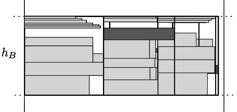
(f) After Stretch

Figure 5: Malformed packings due to inserted or removed items. Operations Sink, Align, and Stretch restore the packing structure.

WidestItems($T,s_{min}$)

returns a set of items $S\subseteq T$ such that $w(i)\geq w(i^{\prime})$ for each $i\in S,i^{\prime}\in T\setminus S$ and $h(S)\in[s_{min},s_{min}+1)$. That is, it picks greedily widest items from $T$ until the total height exceeds $s_{min}$.

Sink($c$)

places big items in container $c$ on a contiguous stack starting from the bottom (gaps due to removed items are closed). See Figures 5(a) to 5(c).

Align($u$)

places the containers of level $u$ according to their actual widths (widest item inside) left-aligned and without gaps. See Figures 5(c) to 5(d). This operation is necessary for the insertion of narrow items treated in the later Section 4.2, but for convenience already presented here.

Stretch($u$)

resolves overlaps occurring when a new item $i$ gets placed into a container $c$ with $w(c)<w(i)\leq w^{R}(c)$. (see Figures  5(f) to 5(e)). Note that the level assignment is according to the LP 2.4 which considers the rounded width $w^{R}(c)$ for a container $c$. The conditions for the insertion of an item (given later in Section 3.2) ensure that only items $i$ with $w(i)\leq w^{R}(c)$ get inserted into a container $c$. Therefore, after Stretch all containers still fit into their level.

Place($g,S$)

packs items in $S$ into appropriate containers of group $g$. Depending on the item type (big or flat), different algorithms are used, which will be present in Sections 3.5.2 and 3.5.3.

InsertContainer (Algorithm 2)

reflects the insertion of the new containers in the LP/ILP-solutions of LP 2.4. To maintain the approximation guarantee, it makes use of the procedure Improve from [18]. Loosely speaking, calling Improve($\alpha$,$x$,$y$) on LP/ILP-solutions $x$, $y$ yields a new solution where the approximation guarantee is maintained and the additive term is reduced by $\alpha$. Further details are given in Section 3.5.4 and Appendix A.

1

2

Input :  $x,y$ fractional and integral solutions to LP($C_{\mathit{con}}^{R}$)

3

4Improve(1,$x$,$y$)

5 Let $P_{i}$ the pattern such that $P_{i}=\{w^{R}(c):1\}$

6 Set $x_{i}:=x_{i}+1$ and $y_{i}:=y_{i}+1$

Algorithm 2 Insertion of a container $c$

3.2 Shift Operation

The insertion of a set of items $S$ into containers of a suitable group $g$ may violate ($\mathcal{I}$5). In this case, the Shift operation modifies the container assignment such that ($\mathcal{I}$1) to ($\mathcal{I}$5) are fulfilled.

The easy case is when $h(g)+h(S)$ does not exceed the upper bound $(h_{B}-1)K_{g}$ from ($\mathcal{I}$5). Then, all items in $S$ can be packed into appropriate containers of $g$. This can be easily seen with the following indirect proof: Assume that item $i\in S$ can not be placed. Then, each of the $K_{g}$ containers is filled with items of total height greater than $h_{B}-1$. Thus, $h(g)+h(S)>K_{g}(h_{B}-1)$, which contradicts ($\mathcal{I}$5).

Now assume that the insertion of items from $S$ exceeds the upper bound by $\Delta>0$ and therefore violates ($\mathcal{I}$5). Basically there are two ways to deal with this situation:

• Except for flexible groups, $K_{g}=2^{l}k$ or $K_{g}=2^{l}(k-1)$. That is, we can not open new containers and thus have to remove items of group $g$ to make room for $S$. When the removed items are the widest of the group $g$, they can be assigned to the group $\mathit{left}(g)$ while maintaining the sorting order ($\mathcal{I}$2).

• The items in $S$ can be placed into new containers if $g$ is flexible and $K_{g}$ not at its upper bound. This procedure is also necessary if there is no group to the left of $g$.

The first of this two shift modes is called left group and the second new container. Further details on both shift modes are given in the following.

Mode: Left group

First, we analyze in which cases we can proceed like that. According to invariant ($\mathcal{I}$3)-($\mathcal{I}$4), there are two flexible groups, namely $(l,A,0)$ and $(l,B,q(l,B))$. In those groups, the shift of items to the left group shall only be performed if a new container can not be opened, i. e. $K_{g}=2^{l}k$ for block $A$ or $K_{g}=2^{l}(k-1)$ for block $B$ ($\mathcal{I}$3)-($\mathcal{I}$4). Furthermore, this shift mode shall also not be used if $g=(l,A,-1)$, that is, $S$ contains items that were shifted out from $(l,A,0)$ in the previous call of shift. Thus the condition for the shift mode left group is:

$$\left(g=(l,A,0)\Rightarrow K_{g}=2^{l}k\right)\wedge\left(g=(l,B,q(l,B))\Rightarrow K_{g}=2^{l}(k-1)\right)\wedge g\neq(l,A,-1)\,.$$

Now, we turn to the changes in the packing. In order to insert the items in $S$, we choose a set of items $S_{out}\subset{I_{L}}^{g}$ and move them to the group $\mathit{left}(g)$. Since the sorting of items over the groups ($\mathcal{I}$2) must be maintained, $S_{out}$ contains widest items of the group $g$. To keep the amount of shifted items small, $S_{out}$ is chosen such that $h(S_{out})$ is minimal but ($\mathcal{I}$5) is fulfilled again. WidestItems$({I_{L}}^{g}\cup S,\Delta)$ (see Section 3.1) is designed exactly for this purpose. Now, we can remove the items $S_{out}$ from the containers and close gaps in the stacks by Sink. Thus there is enough room to place $S$ (note that overlaps are resolved by Stretch, which is part of the Place operation). The shifting process continues with Shift$(\mathit{left}(g),S_{out})$ in order to insert the shifted out items.

Mode: New container

This mode is performed in all remaining cases, i. e. if

$$\left(g=(l,A,0)\wedge K_{g}<2^{l}k\right)\vee\left(g=(l,B,q(l,B))\wedge K_{g}<2^{l}(k-1)\right)\vee~{}g=(l,A,-1)\,.$$

In the first two cases we are allowed to open a new container and therefore have a simple way to maintain ($\mathcal{I}$5) without violating other invariant properties. The last case $g=(l,A,-1)$ results from a shift out of the group $(l,A,0)$ when $K_{(l,A,0)}=2^{l}k$ holds. Then, the newly opened container builds the new leftmost group in block $A$, temporarily called $(l,A,-1)$. In all cases, the residual items are packed into a new container $\bar{c}$ (it will be shown later that one container is enough). The new container gets placed via InsertContainer. Finally, a renaming of groups in block $A$ restores the notation (first group has index $r=0$)

In Algorithm 3, which shows the entire shift algorithm, we require that the group $g$ is suitable for the set of items $S$, according to the following definition:

Definition 3.1 (Suitable group).

For a group $g$, let $w_{min}(g)$ resp. $w_{max}(g)$ denote the width of an item with minimal resp. maximal width in ${I_{L}}^{g}$. Set $w_{min}(\mathit{left}((l,A,0)))=\infty$ and $w_{max}(\mathit{right}((l,B,q(l,B))))=0$. Group $g=(l,X,r)$ is suitable for a new item $i$ if $w(i)\in(2^{-(l+1)},2^{-l}]$, $w_{min}(\mathit{left}(g))\geq w(i)$, and $w_{max}(\mathit{right}(g))<w(i)$.

By the conditions from Definition 3.1, $i$ is inserted into the correct width category ($\mathcal{I}$1) and maintains the sorting over the groups ($\mathcal{I}$2).

1

2

Input : Group $g\in G$

Items $S\subset I_{L}$, where $g$ is suitable for each $i\in S$ (Def. 3.1)

3

4$\Delta=h(g)+h(S)-(h_{B}-1)K_{g}$

5 if $\Delta\leq 0$  then // No violation of invariant ($\mathcal{I}$5)

6       Place($g$,$S$)

7      

8 else

9      

10      if shift mode = left group then

11            

12            $S_{out}$ = WidestItems(${I_{L}}^{g}\cup S$, $\Delta$)

13             Remove $S_{out}$ from $g$

14             Sink($c_{j}$) // For all affected containers $c_{j}$

15             Place($g$,$S$)

16             Shift($\mathit{left}(g),S_{out}$)

17            

18      

19      else if shift mode = new container then

20             Let $\bar{c}$ be new container of $g$

21             Place($g$,$S$)

22             InsertContainer($\bar{c}$)

23            

24            Rename groups in block $A$ // First group gets index 0

25            

26      

27 end if

Algorithm 3 Shift

3.2.1 Sequence of Shift Operations

Figure 6: Shift sequence considered in Lemma 3.2 and Corollary 3.3

According to Algorithm 3 a shift operation can end with a recursive call Shift($\mathit{left}(g),S_{out}$). Note that, due to the procedure WidestItems, $h(S_{out})>h(S)$ can hold. This way a sequence of shift operations can occur, where the height of shifted items grows in each part of the sequence. We consider the shift sequence

$$\textsc{Shift}(g^{0},S^{0}),\textsc{Shift}(g^{1},S^{1}),\ldots,\textsc{Shift}(g^{d-1},S^{d-1}),\textsc{Shift}(g^{d},S^{d})$$

(see Figure 6) and denote the values of $S$, $S_{out}$, and $\Delta$ in the call $\textsc{Shift}(g^{j},S^{j})$ by $S^{j}$, $S_{out}^{j}$, and $\Delta_{j}$. The next lemma states that the total height of the shifted out items $S_{out}^{j}$ grows linearly in $j$, the position in the shift sequence.

Lemma 3.2.

For any $j$ with $0\leq j\leq d$ in the above defined shift sequence, $h(S_{out}^{j})\leq h(S^{0})+j+1\,.$

Proof.

First note that $\Delta_{j}\leq h(S^{j})$ holds for each $j$ by ($\mathcal{I}$5). Further, the function WidestItems($\cdot,\Delta_{j})$ returns a set $S_{out}^{j}$ with $h(S_{out}^{j})<\Delta_{j}+1$. For $j=0$ it holds that $h(S_{out}^{0})<\Delta_{0}+1\leq h(S^{0})+1$. Now suppose $h(S_{out}^{j})\leq h(S^{0})+j+1$ for some $j\geq 0$. Note that $S^{j+1}=S_{out}^{j}$, thus $h(S_{out}^{j+1})<\Delta_{j+1}+1\leq h(S^{j+1})+1=h(S_{out}^{j})+1$. By assumption, $h(S_{out}^{j})\leq h(S^{0})+j+1$ and thus $h(S_{out}^{j+1})\leq h(S^{0})+(j+1)+1$. ∎

Corollary 3.3.

In the shift sequence defined above, it holds that $h(S^{d})\leq h(S^{0})+h_{B}-2$.

Proof.

The maximal total height of $S^{d}$ occurs in the longest possible shift sequence, that is, when $g^{0}=(l,B,q(l,B))$, $g^{d-1}=(l,A,0)$, and $g^{d}=(l,A,-1)$ hold. Note that $S^{d}=S_{out}^{d-1}$.

We have $d=q(l,A)+q(l,B)+2$ for some $l\in W$ and with Lemma 2.7 (Equations (2.1) and (2.2)) $d\leq 16\omega/\epsilon+2\omega$. Lemma 3.2 gives $h(S_{out}^{d-1})\leq h(S^{0})+(d-1)+1\leq h(S^{0})+16\omega/\epsilon+2\omega$. It remains to show $16\omega/\epsilon+2\omega\leq h_{B}$, which follows by definition of $\omega$ and $h_{B}$. ∎

Note that Corollary 3.3 implies that shifting a single item $i_{t}$ into a group, we have $h(S^{d})\leq h(i_{t})+h_{B}-2\leq h_{B}-1$. Therefore, one container is enough to pack all items in $S^{d}$ arriving in $(l,A,-1)$.

3.3 ShiftA

In Section 3.5.1 we need an operation which moves one group from block $B$ to block $A$ within one category $l\in W$. This ShiftA operation, closely related to the dynamic rounding technique adapted from [4], is considered in the following.

The characteristic property of groups in block $B$ is the number of containers $2^{l}(k-1)$, while groups in block $A$ have $2^{l}k$ containers (invariant properties ($\mathcal{I}$3)- ($\mathcal{I}$4), except for flexible groups). ShiftA enlarges the group $(l,B,0)$ by $2^{l}$ additional containers such that it can act as the new $(l,A,q(l,A))$ group. To fulfill ($\mathcal{I}$5), widest items (similar to Shift) are moved from group $(l,B,1)$ to $(l,B,0)$ such that ($\mathcal{I}$5) is fulfilled for the group $(l,B,0)$ with $2^{l}$ additional containers. As items are taken from $(l,B,1)$, widest items from $(l,B,2)$ have to be shifted to $(l,B,1)$ and so on.

It might be the case that the removal of items from the last group $(l,B,q(l,B))$ leads to a violation of ($\mathcal{I}$5) since there are too many containers for the total height of the residual items. Then, some containers have to be emptied and removed. At the extreme, all containers of the group get removed and thus $(l,B,q(l,B)-1)$ becomes the new group $(l,B,q(l,B))$ via renaming.

Note that each of the $2^{l}$ new containers of the new group $(l,A,q(l,A))$ has width at most $2^{-l}$ and thus they can be placed in one level of height $h_{B}$ in the strip. Algorithm 4 shows the steps explained above. Thereby, two auxiliary algorithms for the insertion and removal of containers (Algorithms 5 to 6 ) occur, which are given in the following subsection.

1

2

Input : Width category $l\in W$

3

4Let $g_{i}=(l,B,i)$ for $0\leq i\leq q(l,B)$

5 Let $c_{1},\ldots c_{2^{l}}$ be new containers of group $g_{0}$

6

7for i=0 …q(l,B)-1 do

8       $u=\begin{cases}2^{l}k(h_{B}-1)&\mbox{if }i=0\\ 2^{l}(k-1)(h_{B}-1)&\mbox{if }i>0\end{cases}$

9       $s_{min}=u-h(g_{i})-1$

10      

11      $S$ = WidestItems(${I_{L}}^{g_{i+1}}$, $s_{min}$)

12       Remove $S$ from $g_{i+1}$

13       Sink($c_{j}$) // For all affected containers $c_{j}$

14       Place($S$,$g_{i}$)

15      

16 end for

17Insert containers $c_{1},\ldots c_{2^{l}}$ via Algorithm 5

18 Rename $g_{0}$ to $(l,A,q(l,A)+1)$

19

 // If necessary, remove containers from $(l,B,q(l,B))$

20 $\Delta=(K_{g_{q(l,B)}}-1)(h_{B}-1)-h(g_{q(l,B)})$

21 if $\Delta>0$ then

22       Empty $\left\lceil{\frac{\Delta}{h_{B}-1}}\right\rceil$ containers

23       Remove each of them via Algorithm 6

24      

25

26Renaming

Algorithm 4 ShiftA

The next lemma states how many containers have to be removed from a flexible group when the total height of items falls below the lower bound of ($\mathcal{I}$5). Note that Algorithm 4 behaves exactly accordingly to the lemma in Line 4.

Lemma 3.4.

Assume that $h(g)=(K_{g}-1)(h_{B}-1)-\Delta$ for a group $g$ and $\Delta>0$. Removing $\lceil{\frac{\Delta}{h_{B}-1}}\rceil$ containers restores ($\mathcal{I}$5).

Proof.

Let $\delta=\left\lceil{\frac{\Delta}{h_{B}-1}}\right\rceil$. It is easy to show that $h(g)\geq(K_{g}-\delta-1)(h_{B}-1)$. ∎

3.3.1 Insertion and Deletion of Containers

As a result of the ShiftA procedure, for a category $l$ there are $2^{l}$ containers that have to be inserted into the packing. Instead of using Algorithm 2 for each single container, we rather use a slightly modified algorithm presented below. Since all containers have rounded width $w^{R}(c)\leq 2^{-l}$, they fit into one level of the strip. Hence, one single call of Improve, followed by a change of the LP/ILP-solution, is enough. Algorithm 5 shows the steps for the insertion of $2^{l}$ new containers.

1

2

Input : $x,y$ fractional and integral solutions to LP($C_{\mathit{con}}^{R}$)

3

4Improve(1,$x$,$y$)

5 Let $P_{i}$ the pattern s.t. $P_{i}=\{w^{R}(c_{1}):1,w^{R}(c_{2}):1,\ldots,w^{R}(c_{2^{l}}):1\}$

6 Set $x_{i}:=x_{i}+1$ and $y_{i}:=y_{i}+1$

Algorithm 5 Insertion of containers $c_{1},\ldots,c_{2^{l}}$ for ShiftA

Furthermore, containers of group $(l,B,q(l,B))$ may get deleted at the end of the ShiftA algorithm. Analogously to the insertion of containers, modifications in the LP/ILP-solutions are necessary to reflect the change of the packing. See Algorithm 6.

1

2

Input : $x,y$ fractional and integral solutions to LP($C_{\mathit{con}}^{R}$)

3

4Let $P_{i}$ a pattern containing $w^{R}(c)$

5 Let $P_{j}=P_{i}\setminus w^{R}(c)$ be the pattern without $w^{R}(c)$.

6 Set $x_{i}:=x_{i}-1$ and $y_{i}:=y_{i}-1$

7 Set $x_{j}:=x_{j}+1$ and $y_{j}:=y_{j}+1$

Algorithm 6 Deletion of a container $c$ for ShiftA

3.4 Operations Maintain Properties

In this section we show that the operations Shift and ShiftA maintain all invariant properties (Lemma 3.5). Further, in Lemma 3.6 it is shown that also the LP/ILP-solutions (modified by Algorithms 2, 5, and 6) stay feasible.

Lemma 3.5.

Assume that the ($\mathcal{I}$1)- ($\mathcal{I}$5) are fulfilled by a container assignment $\mathit{con}$ and a rounding function $R$. Applying one of the operations Shift($g$,$S$) for any $g\in G$ and $S$ with $h(S)\leq h_{B}-1$ and $g$ is suitable for all $i\in S$, and ShiftA($l$) for any $l\in W$ maintains ($\mathcal{I}$1)- ($\mathcal{I}$5).

Proof.

Implicitly, the operations modify both functions: The container assignment is changed in the Shift and ShiftA algorithm due to the removal or placing of item sets. The rounding function changes when new containers get assigned.

Shift

Let $g=(l,X,r)$. Each item assigned to group $g$ by Shift is suitable for $g$ or comes from the group $\mathit{right}(g)$. In the first case, ($\mathcal{I}$1)- ($\mathcal{I}$2) hold by Definition 3.1, in the latter case by the fact that only widest items are moved to the left within the same category.

The number of containers only changes in the second shift mode (Lines 3 to 3 ). The preconditions of the respective shift mode ensure that either an additional container does not violate ($\mathcal{I}$3)- ($\mathcal{I}$4) since $g$ is a flexible group, or the new container belongs to group $(l,A,-1)$. After the renaming this group becomes $(l,A,0)$, has only one container, and thus fulfills ($\mathcal{I}$3). In the latter case groups in block $B$ remain unchanged, thus in all cases ($\mathcal{I}$3)- ($\mathcal{I}$4) are maintained.

Finally, the algorithm is designed to maintain property ($\mathcal{I}$5) by shifting items of appropriate height. If $\Delta\leq 0$, then the new total height of items in group $g$ is $h(g)+h(S)=\Delta+(h_{B}-1)K_{g}\leq(h_{B}-1)K_{g}$. On the other hand, $h(g)+h(S)\geq(K_{g}-1)(h_{B}-1)$ holds by the assumption that ($\mathcal{I}$5) is fulfilled beforehand and $h(S)\geq 0$. Now assume $\Delta>0$. We analyze both shift modes separately.

Mode: Left group

We have to show that the total height of items after the removal of $S_{out}$ and insertion of $S$ lies in the interval $[(h_{B}-1)(K_{g}-1),(h_{B}-1)K_{g}]$. Recall $\Delta=h(g)+h(S)-(h_{B}-1)K_{g}$. It holds $h(S_{out})\geq\Delta$ and thus

$$h(g)-h(S_{out})+h(S)\leq h(g)-\Delta+h(S)=(h_{B}-1)K_{g}\,.$$

On the other side, $h(S_{out})<\Delta+1$ and thus

$$h(g)-h(S_{out})+h(S)>h(g)-\Delta-1+h(S)=(h_{B}-1)K_{g}-1\geq(h_{B}-1)(K_{g}-1)\,,$$

where the last inequality follows by $h_{B}\geq 2$. Hence, property ($\mathcal{I}$5) is fulfilled.

Mode: New container

In the case that a new container gets inserted into one of the flexible groups $(l,A,0)$ or $(l,B,q(l,B))$, the number of containers $K_{g}$ is changed to $K_{g}^{\prime}=K_{g}+1$. We have to show that the new total height of items per group $h(g)+h(S)$ lies in the interval $[(K_{g}^{\prime}-1)(h_{B}-1),K_{g}^{\prime}(h_{B}-1)]$. Since $\Delta>0$, it holds that $h(g)+h(S)\geq K_{g}(h_{B}-1)=(K_{g}^{\prime}-1)(h_{B}-1)$. By assumption, $h(g)\leq K_{g}(h_{B}-1)$ and $h(S)\leq h_{B}-1$ hold, and thus $h(g)+h(S)\leq K_{g}(h_{B}-1)+(h_{B}-1)=(K_{g}+1)(h_{B}-1)=K_{g}^{\prime}(h_{B}-1)$.

The remaining case is $g=(l,A,-1)$. Then, we insert a single container into the empty group $g$ and have to show $h(S)\in[(K_{g}^{\prime}-1)(h_{B}-1),K_{g}^{\prime}(h_{B}-1)]$. Since $K_{g}^{\prime}=1$, the lower bound holds obviously for any $h(S)\geq 0$. Again by assumption, $h(S)\leq h_{B}-1=K_{g}^{\prime}(h_{B}-1)$.

ShiftA

Since items are moved between groups of the same category, ($\mathcal{I}$1) can not be violated. Let $g_{i}=(l,B,i)$ for $0\leq i\leq q(l,B)$. Again, widest items are removed from one group $g_{i+1}$ and then assigned to group $g_{i}$, where $g_{i}=\mathit{left}(g_{i+1})$ and therefore ($\mathcal{I}$2) is maintained. The number of containers of group $g_{0}$ is enlarged by $2^{l}$ to $2^{l}(k-1)+2^{l}=2^{l}k$. Hence, $g_{0}$ can be moved to block $A$ afterwards while maintaining ($\mathcal{I}$3). In block $B$, the number of containers per group is not changed, except for $g_{q(l,B)}$, whose number of containers might be decreased. But since $(l,B,q(l,B))$ is a flexible group, ($\mathcal{I}$4) holds anyway.

The crucial part is again to show that ($\mathcal{I}$5) is fulfilled after the ShiftA operation. The new total height of items in group $g_{i}$ is $h^{\prime}(g_{i})=h(g_{i})+h(S)$ and due to the procedure WidestItems we have $h^{\prime}(g_{i})=h(g_{i})+h(S)\leq h(g_{i})+s_{min}+1=u$ and $h^{\prime}(g_{i})=h(g_{i})+h(S)\geq h(g_{i})+s_{min}=u-1$.

In the case $i=0$, we have to show $(2^{l}k-1)(h_{B}-1)\leq h^{\prime}(g_{0})\leq 2^{l}k(h_{B}-1)$ as $g_{0}$ shall act as new $(l,A,q(l,A))$ group. By definition of $u$, it holds that $h^{\prime}(g_{0})\leq u=2^{l}k(h_{B}-1)$ and $h^{\prime}(g_{0})\geq u-1=2^{l}k(h_{B}-1)-1\geq(2^{l}k-1)(h_{B}-1)$, where the last inequality follows by $h_{B}-1\geq 1$.

For $1\leq i<q(l,B)$, the value of $h^{\prime}(g_{i})$ has to be in the interval $[(2^{l}(k-1)-1)(h_{B}-1),2^{l}(k-1)(h_{B}-1)]$. We get similarly $h^{\prime}(g_{i})\leq u=2^{l}(k-1)(h_{B}-1)$ and again with $h_{B}-1\geq 1$ it follows that $h^{\prime}(g_{i})\geq u-1=2^{l}(k-1)(h_{B}-1)-1\geq(2^{l}(k-1)-1)(h_{B}-1)$.

It remains to analyze the case $i=q(l,B)$. Items from group $g_{q(l,B)}$ are shifted to group $g_{q(l,B)-1}$ in order to fulfill ($\mathcal{I}$5) for $g_{q(l,B)-1}$. Therefore, the loss of total height in group $g_{q(l,B)}$ is at most

$$s_{min}+1 =u-h(g_{q(l,B)-1})$$

$$\leq 2^{l}k(h_{B}-1)-h(g_{q(l,B)-1})$$

$$\leq 2^{l}k(h_{B}-1)-(2^{l}(k-1)-1)(h_{B}-1)$$

$$=(2^{l}+1)(h_{B}-1)$$ (3.1)

which can not be compensated by another shift, since $(l,B,q(l,B))$ has no right neighbor. Instead, decreasing the number of containers will repair property ($\mathcal{I}$5). Maybe, the loss of items can be compensated (partially) because the previous total height $h(g)$ was greater than $(K_{g_{q(l,B)}}-1)(h_{B}-1)$, the lower bound of ($\mathcal{I}$5). For this purpose, define the actual amount of height $\Delta$ that is required to fulfill ($\mathcal{I}$5): Let $\Delta=(K_{g_{q(l,B)}}-1)(h_{B}-1)-h^{\prime}(g_{q(l,B)})$. We have

$$h^{\prime}(g_{q(l,B)}) \geq h(g_{q(l,B)})-(s_{min}+1)$$

$$\geq(K_{g_{q(l,B)}}-1)(h_{B}-1)-(2^{l}+1)(h_{B}-1)$$ eq. (3.4)

$$=(K_{g_{q(l,B)}}-2^{l}-2)(h_{B}-1)$$

and therefore

$$\Delta =(K_{g_{q(l,B)}}-1)(h_{B}-1)-h^{\prime}(g_{q(l,B)})$$

$$\leq(K_{g_{q(l,B)}}-1)(h_{B}-1)-(K_{g_{q(l,B)}}-2^{l}-2)(h_{B}-1)$$

$$=(K_{g_{q(l,B)}}-K_{g_{q(l,B)}}+2^{l}+1)(h_{B}-1)$$

$$=(2^{l}+1)(h_{B}-1)\,.$$

Clearly, if $\Delta\leq 0$, nothing has to be done since ($\mathcal{I}$5) is already fulfilled. Assuming $\Delta>0$, by Lemma 3.4 the removal of

$$\left\lceil\frac{\Delta}{h_{B}-1}\right\rceil\leq\left\lceil\frac{(2^{l}+1)(h_{B}-1)}{h_{B}-1}\right\rceil=\left\lceil 2^{l}+1\right\rceil$$ (3.2)

containers is enough. Since Algorithm 4 behaves exactly like this starting from Line 4, we can conclude that ($\mathcal{I}$5) is fulfilled for group $g_{q(l,B)}$ by adjusting the number of containers appropriately. ∎

Lemma 3.6.

Assume that the ($\mathcal{I}$1)- ($\mathcal{I}$5) are fulfilled by a container assignment $\mathit{con}$ and a rounding function $R$. Let $x$ and $y$ be corresponding LP/ILP-solutions. Applying one of the operations Shift, ShiftA defines new functions $\mathit{con}^{\prime}$, $R^{\prime}$ and new solutions $x^{\prime},y^{\prime}$. The solutions $x^{\prime},y^{\prime}$ are feasible for the LP defined on the new rounded container instance $C_{\mathit{con}^{\prime}}^{R^{\prime}}$.

Proof.

Again, we look at each operation separately.

Shift (Mode: Left group)

The conditions from Definition 3.1 ensure that no item that is inserted into a container increases the rounded width of that container. Therefore, each container in $C_{\mathit{con}^{\prime}}^{R^{\prime}}$ has a smaller or equal width than in $C_{\mathit{con}}^{R}$, i. e. $w^{R^{\prime}}(c)\leq w^{R}(c)$.

Since in this case the cardinalities of the rounding groups do not change (no container gets inserted or removed), the right hand side in LP 2.4 does not change. All configurations of $C_{\mathit{con}}^{R}$ can be transformed into feasible configurations of $C_{\mathit{con}^{\prime}}^{R^{\prime}}$.

Shift (Mode: New container)

In this case, a new container $\bar{c}$ is placed in a new level. The algorithm InsertContainer reflects this action in the LP/ILP-solution: For the pattern $P_{i}$ that contains the rounded width of $\bar{c}$ once the corresponding values $x_{i}$ and $y_{i}$ are increased by one.

ShiftA

The ShiftA algorithm can be seen as a series of shift operations where each operation affects two neighboring groups. The new containers get inserted via Algorithm 5, the removal of containers is done by Algorithm 6. Both algorithms are similar to InsertContainer. Therefore, the claim can be shown analogously to Shift. ∎

3.5 Insertion Algorithms

Before we can give the entire algorithms for the insertion of a big or flat item, we have to deal with another problem: Remember that the parameter $k$, which controls the group sizes by ($\mathcal{I}$3)- ($\mathcal{I}$4), depends on $\operatorname{SIZE}(I_{L}(t))$ and thus changes over time. Hence, for this section we use the more precise notation $k(t)=\left\lfloor{\frac{\epsilon}{4\omega h_{B}}\operatorname{SIZE}(I_{L}(t))}\right\rfloor$. Let $\kappa(t)=\frac{\epsilon}{4\omega h_{B}}\operatorname{SIZE}(I_{L}(t))$.

At some point $t+1$, the value of $k(t+1)$ will increase such that $k(t+1)=k(t)+1$. Obviously, we can not rebuild the whole container assignment to fulfill the new group sizes required by ($\mathcal{I}$3)- ($\mathcal{I}$4) according to $k(t+1)$. Instead, the block structure is exactly designed to deal with this situation. By adjusting the ratio of the block sizes of $A$ and $B$, the problem mentioned above can be overcome. This dynamic block balancing technique was developed in [4, Sec. 3.3] and is described in the following section.

3.5.1 Dynamic Block Balancing

All groups of block $A$ that fulfill invariant ($\mathcal{I}$3)- ($\mathcal{I}$4) with parameter $k(t)$ can act as groups of block $B$ with parameter $k(t)+1=k(t+1)$. So assuming that block $B$ is empty, renaming block $A$ into $B$ fulfills the invariant properties. Note that with ShiftA we have an operation that transfers a single group from block $B$ to $A$.

Therefore, we have to ensure that whenever the (integer) value of $k(t)$ is willing to increase (i. e. $\kappa(t)$ has a fractional value close to one), the block $B$ is almost empty. Let the block balance be defined as $bb(t)=\frac{A(t)}{A(t)+B(t)}$, where $A(t)$ and $B(t)$ denote the number of groups in the respective block summing over all categories. Note that $bb(t)$ equals one if and only if the $B$-block is empty.

Let $\mathit{frac}\left({\kappa(t)}\right)\in[0,1)$ be the fractional part of $k(t)$. To adjust the block balance to the value of $\mathit{frac}\left({\kappa(t)}\right)$, we partition the interval $[0,1)$ into smaller intervals $J_{i}$:

$$J_{i}=\left[\frac{i}{A(t)+B(t)},\frac{i+1}{A(t)+B(t)}\right)\hskip 20.0pt\text{for }i=0,\ldots,A(t)+B(t)-1$$

Algorithm 7 shows the block balancing algorithm: A number $d$ of groups is moved from block $B$ to $A$ such that afterwards $bb(t)\in J_{i}\iff\mathit{frac}\left({\kappa(t)}\right)\in J_{i}$. Hence, block $B$ is almost empty when $k(t)$ is willing to increase.

1

2Let $i$ s.t. $\mathit{frac}\left({\kappa(t)}\right)\in J_{i}$

3 Let $j$ s.t. $bb(t)\in J_{j}$

4 Set $d=i-j\bmod A(t)+B(t)$

5 for p=0 …d-1 do

6       if $j+p=A(t)+B(t)$  then // Block $B$ is empty

7             Rename Block $A$ to Block $B$

8            

9       shiftA($l$) // for any suitable category $l$

10      

11 end for

12

Algorithm 7 Block Balancing Algorithm

Lemma 3.7.

Assume that $\mathit{frac}\left({\kappa(t)}\right)\in J_{i}$. At the end of Algorithm 7 it holds that $bb^{*}(t)\in J_{i}$, where $bb^{*}(t)$ is the block balance after shifting $d$ groups from $B$ to $A$.

Proof.

Let $J_{j}$ be the interval containing $bb(t)$, the block balance before the ShiftA operations. We have to show that after performing $d=i-j\bmod A(t)+B(t)$ ShiftA operations, it holds that $bb^{*}(t)\in J_{i}$. Each call of ShiftA moves one group from $B$ to $A$. Let $bb^{\prime}(t)$ be the block balance after one single call of ShiftA. We have

$$bb^{\prime}(t)=bb(t)+\frac{1}{A(t)+B(t)}\geq\frac{j}{A(t)+B(t)}+\frac{1}{A(t)+B(t)}=\frac{j+1}{A(t)+B(t)}$$

and

$$bb^{\prime}(t)=bb(t)+\frac{1}{A(t)+B(t)}<\frac{j+1}{A(t)+B(t)}+\frac{1}{A(t)+B(t)}=\frac{j+2}{A(t)+B(t)}\,.$$

Hence, $bb^{\prime}(t)\in J_{j+1}$, where $j+1$ can be seen as performed modulo $A(t)+B(t)$: When $j+p=A(t)+B(t)$ for $0\leq p\leq d-1$, the algorithm renames block $A$ to $B$. Note that block $B$ is empty at this time since $p$ calls of ShiftA were performed previously. After renaming, the $A$ block is empty and the block balance lies in the interval $J_{0}$. As $bb^{*}(t)$ denotes the block balance after $d$ calls of ShiftA, the interval index of $bb^{*}(t)$ equals $j+d\bmod A(t)+B(t)=j+(i-j\bmod A(t)+B(t))\bmod A(t)+B(t)=i\,.$ ∎

For the migration analysis it is important how many groups are shifted between blocks. The next lemma shows that the total number of groups shifted for the insertion of a set $M$ grows proportional with $\operatorname{SIZE}(M)$.

Lemma 3.8.

Let $t,t^{\prime}$ be two time steps and $M$ the set of items inserted in between, i. e. $I_{L}(t^{\prime})=I_{L}(t)\cup M$. Assume that each item $i\in M$ causes one call of Algorithm 7 and let $d_{i}$ be the parameter $d$ for item $i$. It holds that $\sum_{i\in M}d_{i}\leq\frac{8+\epsilon}{2h_{B}}\operatorname{SIZE}(M)+1$.

Proof.

By definition, $\kappa(t)$ grows linearly in $\operatorname{SIZE}(I_{L}(t))$, thus $\kappa(t^{\prime})-\kappa(t)=\allowbreak\frac{\epsilon}{4\omega h_{B}}\operatorname{SIZE}(M)$. We obtain an upper bound for the difference of the fractional parts: $\mathit{frac}\left({\kappa(t^{\prime})}\right)-\mathit{frac}\left({\kappa(t)}\right)\leq\frac{\epsilon}{4\omega h_{B}}\operatorname{SIZE}(M)$.

By Lemma 2.7, at each time $t$ the total number of groups $A(t)+B(t)$ is at most $\frac{16\omega+2\omega\epsilon}{\epsilon}$. Hence, all intervals $J_{i}$ have the length $\frac{1}{A(t)+B(t)}\geq\frac{\epsilon}{16\omega+2\omega\epsilon}$. From Lemma 3.7 we know that $bb(t)\in J_{i}\iff\mathit{frac}\left({\kappa(t)}\right)\in J_{i}$ after each run of Algorithm 7. The total number of intervals that can lie between $\kappa(t^{\prime})$ and $\kappa(t)$ can thus be bounded as follows:

$$\sum_{i\in M}d_{i}\leq\left\lceil{\frac{\mathit{frac}\left({\kappa(t^{\prime})}\right)-\mathit{frac}\left({\kappa(t)}\right)}{\frac{\epsilon}{16\omega+2\omega\epsilon}}}\right\rceil\leq\left\lceil{\frac{\frac{\epsilon}{4\omega h_{B}}\operatorname{SIZE}(M)}{\frac{\epsilon}{16\omega+2\omega\epsilon}}}\right\rceil\leq\frac{8+\epsilon}{2h_{B}}\operatorname{SIZE}(M)+1$$

∎

3.5.2 Insertion of Big Items

The insertion algorithm for a big item $i_{t}$ given in Algorithm 8 is very simple: Basically, the insertion of item $i_{t}$ is done by the Shift algorithm called with a suitable group. Afterwards, the block balancing presented in Section 3.5.1 is performed.

1

Input : Item $i_{t}\in I_{L}$

2

3Find suitable group $g=(l,X,r)$ according to Definition 3.1

4 Shift($g,\{i_{t}\}$)

5 BlockBalancing

6

Algorithm 8 Insertion of a big item

It remains to give the Place algorithm which is used as a subroutine in Shift. For each item $i$ to be inserted, Algorithm 9 looks for a container where $i$ can be added without overfilling the container, places the item on top of the stack and calls Stretch to resolve overlaps.

1

2

3

Input : Group $g$, set of big items $S$

4

5Let $H(c)=\sum_{i\in I_{L}:\mathit{con}(i)=c}h(i)$

6

7for $i\in S$ do

8       Find container $c$ with $R(c)=g$ and $H(c)\leq h_{B}-h(i)$

9       Place $i$ on top of the stack for big items in $c$

10       Stretch(u), where $u$ is the level of $c$

11      

Algorithm 9 Placing of big items

3.5.3 Insertion of Flat Items

The main difficulty of flat items becomes clear in the following scenario: Imagine that flat items of a group $g$ are elements of $S_{out}=\textsc{WidestItems}(g,\Delta)$ in a shifting process. Remember that generally each container from which items are removed has to be sinked, i. e. at most $\left|{S_{out}}\right|$ containers. In case of big items, due to their minimum height $\epsilon$ we get $\left|{S_{out}}\right|\leq\lfloor{\Delta/\epsilon}\rfloor$. In contrast, flat items can have an arbitrary small height and thus no such bound is possible. But Sink on all $K_{g}$ containers would lead to unbounded migration (since $K_{g}$ depends on $\operatorname{SIZE}(I_{L})$). Therefore, we aim for a special packing structure that avoids the above problem of sinking too many containers.

Like shown in Figure 1(a), flat items build a sorted stack at the top of the container such that the least wide item is placed at the top edge. Thereby, widest items can be removed from the container without leaving a gap. To maintain the sorting, we introduce a buffer for flat items called $F$-buffer. It is located in a rectangular segment of width 1 and height $\omega y$, somewhere in the packing, where $y=\left|{G}\right|\epsilon^{2}+\epsilon$. Note that the additional height for the F-buffer is bounded by $\omega y=\mathcal{O}\left(\epsilon\left(\log 1/\epsilon\right)^{2}\right)$. The internal structure of the F-buffer is shown in Figure 7: For each category $l$ there are $2^{l}$ slots in one level of height $y$. Items can be placed in any slot of their category.

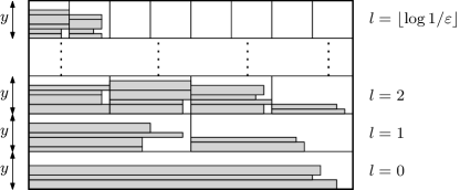
Figure 7: F-buffer contains $2^{l}$ slots of height $y$ for each category $l$.

An incoming flat item may overflow the F-buffer, more precisely, the level of one category in the F-buffer. For this purpose, Algorithm 10 iterates over all groups $g_{q},g_{q-1},\ldots,g_{0}$ of this category, where $g_{q}$ is the rightmost and $g_{0}$ the leftmost group. For each group, the set $S$ contains those items in the F-buffer for which $g$ is a suitable group. The set $S$ is split into smaller subsets of total height at most 1, then each subset gets inserted via a single call of Shift.

1

2

Input : Flat item $i_{t}\in I_{L}$ of category $l$

3

4if $i_{t}$ can be placed in the F-buffer then

5       Place $i_{t}$ in the F-buffer

6      

7 else

8       Let $B(l)$ be the set of items in the buffer slots of category $l$

9       for $j=q(l,A)+q(l,B)+1,\ldots,0$ do

10             Let $g_{j}=\begin{cases}(l,A,j)&j\leq q(l,A)\\ (l,B,j-q(l,A)-1)&j>q(l,A)\end{cases}$

11             Let $S=\{i\in B(l)\mid g_{j}\text{ is suitable for }i\}$

12             Let $S_{1},\ldots,S_{n}$ be partition of $S$ with $h(S_{r})\in(1-\epsilon,1]$ for all $1\leq r\leq n$.

13             for $r=1,\ldots,n$ do

14                   Shift($g_{j}$,$S_{r}$)

15                  

16            Remove $S$ from $B(l)$

17            

18      BlockBalancing

19      

Algorithm 10 Insertion of a flat item

Algorithm 11 shows Place for flat items, required for Shift: The set of flat items $S$ gets partitioned into sets $S_{j}$ each of total height at most 1. Then, each set $S_{j}$ is placed into a container analogously to Algorithm 9. Thereby, the stack of flat items needs to be resorted.

1

2

Input : Group $g$, set of flat items $S$

3

4Let $H(c)=\sum_{i\in I_{L}:\mathit{con}(i)=c}h(i)$

5 Let $S_{1},\ldots,S_{n}$ be partition of $S$ with $h(S_{r})\in(1-\epsilon,1]$ for all $1\leq r\leq n$.

6

7for $j=1,\ldots,n$ do

8       Find container $c$ with $R(c)=g$ and $H(c)\leq h_{B}-h(S_{j})$

9       Add $S_{j}$ to the stack of flat items and resort the stack

10       Stretch(u), where $u$ is the level of $c$

11      

Algorithm 11 Placing of flat items

By choice of $y$, the slot height of the F-buffer, we get the following observation required for a later proof:

Lemma 3.9.

The for-loop in Line 10 of Algorithm 10 iterates at most $\mathcal{O}\left(1/\epsilon\right)$ times.

Proof.

The number of iterations is $n\leq\left\lceil{\frac{h(S)}{1-\epsilon}}\right\rceil$. Thus is is enough to show $h(S)\leq\mathcal{O}\left(1/\epsilon\right)$. Each category $l$ has $2^{l}$ slots of height $y=\left|{G}\right|\epsilon^{2}+\epsilon$. By Lemma 2.7 it follows $\left|{G}\right|\epsilon^{2}\leq 16+2\epsilon$ and thus $y\leq 17$. Further, the maximum slot number is $2^{\left\lfloor{\log 1/\epsilon}\right\rfloor}\leq 1/\epsilon$, therefore $h(S)\leq 17/\epsilon$. ∎

3.5.4 Online-Approximation Guarantee

In Section 3.4 we shows that single Shift- and ShiftA-operations maintain the invariant properties. This holds for Algorithms 8 and 10 as well.

Lemma 3.10.

Algorithms  8 and 10 maintain all invariant properties and the LP/ILP-solutions stay feasible.

Proof.

Both algorithms use the Shift operation to insert new items. In Lemma 3.5 we showed that this operation maintains the invariant properties if applied with a set $S$ of items with $h(S)\leq h_{B}-1$. Thus, the claim follows by Lemma 3.5 if we can show the latter condition.

We show that for the first call $\textsc{Shift}(g^{0},S^{0})$ it holds that $h(S^{0})\leq 1$. Then, $h(S)\leq h_{B}-1$ follows by Lemma 3.2 and Corollary 3.3. In case of big items (Algorithm 8), $S^{0}$ contains a single item, which has maximum height 1. For flat items (Algorithm 10), the partition of the set $S$ ensures that Shift is only called with items of total height 1.

Afterwards both algorithms call the block balancing Algorithm 7. Here, the crucial operation is ShiftA, but Lemma 3.5 already gives the claim. Also by Lemma 3.5, all changes to the LP/ILP-solutions result in new feasible solutions. ∎

However, since the packing height can increase due new containers, also the level assignment gets changed in order to fulfill the approximation guarantee. Here, the crucial operation is Improve called in Algorithms 2, 5, and 6 which we analyze in the following. The next theorem is a modified version of Theorem 3 in [4] and justifies that we can apply Improve on suitable LP/ILP-solutions $x$, $y$ to obtain a solution with reduced additive term. The proof of Theorem 3.11 is moved to Appendix A.

For a vector $x$, let $\mathrm{nnz}(x)$ denote the number of non-zero components. Let $\delta$ be a parameter specified later. By Theorem 2.8, we have $\operatorname{OPT}(C_{\mathit{con}}^{R})\leq(1+\epsilon^{\prime})\operatorname{OPT}(I_{L})+z$ for $\epsilon^{\prime}=4\epsilon$ and $z=\mathcal{O}\left(1/\epsilon^{4}\right)$. Let $\Delta=(1+\epsilon^{\prime})(1+\delta)-1$ and $m$ be the number of constraints in LP 2.4. Since there is exactly one constraint for each occurring width (group), by Lemma 2.7 $m\leq\frac{16\omega}{\epsilon}+2\omega$. Finally, let $D=\Delta\operatorname{OPT}(I_{L})+m+(1+\delta)z$. With the above definitions, we have

$$(1+\epsilon)\operatorname{OPT}(C_{\mathit{con}}^{R})\leq(1+\Delta)\operatorname{OPT}(I_{L})+(1+\epsilon)z\,.$$ (3.3)

Theorem 3.11.

Given a rounded container instance $C_{\mathit{con}}^{R}$ and an LP defined for $C_{\mathit{con}}^{R}$, let $\delta>0$, $\alpha\in\mathbb{N}$, and $x$ be a fractional solution of the LP with

$$\left\lVert x\right\rVert_{1} \leq(1+\Delta)\operatorname{OPT}(I_{L})+(1+\delta)z\,,$$ (3.4)

$$\left\lVert x\right\rVert_{1} \geq 2\alpha\left(\tfrac{1}{\delta}+1\right)\,,$$ (3.5)

$$\left\lVert x\right\rVert_{1} =(1+\delta^{\prime})\operatorname{LIN}(C_{\mathit{con}}^{R})\hskip 12.0pt\text{for }\delta^{\prime}>0\,.$$ (3.6)

Let $$y$$ be an integral solution of the LP with

$$\left\lVert y\right\rVert_{1} \geq(m+2)\left(\tfrac{1}{\delta}+2\right)\,,$$ (3.7)

$$\left\lVert y\right\rVert_{1} \leq(1+2\Delta)\operatorname{OPT}(I_{L})+2(1+\delta)z+m\,.$$ (3.8)

Further, let $\mathrm{nnz}(x)=\mathrm{nnz}(y)\leq D$ and $x_{i}\leq y_{i}$ for all $1\leq i\leq n$.

Then, algorithm Improve($\alpha$) on $x$ and $y$ returns a new fractional solution $x^{\prime}$ with $\left\lVert x^{\prime}\right\rVert_{1}\leq(1+\Delta)\operatorname{OPT}(I_{L})+(1+\delta)z-\alpha$ and also a new integral solution $y^{\prime}$ with $\left\lVert y^{\prime}\right\rVert_{1}\leq(1+2\Delta)\operatorname{OPT}(I_{L})+2(1+\delta)z+m-\alpha$. Further, $\mathrm{nnz}(x^{\prime})=\mathrm{nnz}(y^{\prime})\leq D$, and for each component we have $x^{\prime}_{i}\leq y^{\prime}_{i}$. The number of levels to change in order to obtain the new packing corresponding with $y^{\prime}$ is bounded by $\mathcal{O}\left(m/\delta\right)$.

Theorem 3.12.

Assuming $\operatorname{SIZE}(I_{L}(t))\geq\frac{4\omega h_{B}}{\epsilon}(h_{B}+1)$, Algorithms 8 and 10 are AFPTASs for the insertion of big and flat items with asymptotic ratio $1+2\Delta$ for $\Delta\in\mathcal{O}\left(\epsilon\right)$.

Proof.

Approximation Guarantee

Let $\Delta,\epsilon^{\prime},z,m$ be defined as above and set $\delta=\epsilon$. Then, $\Delta=4\epsilon+\epsilon+\epsilon^{2}=\mathcal{O}\left(\epsilon\right)$. We show by induction that the algorithms maintain a packing of height $h$ with

$$h\leq(1+2\Delta)\operatorname{OPT}(I_{L})+2(1+\epsilon)z+m\,.$$ (3.9)

Suppose that the packing corresponds with $x$ and $y$, which are fractional/integer solutions to $LP(C_{\mathit{con}}^{R})$ such that $\left\lVert x\right\rVert_{1}=(1+\epsilon)\operatorname{LIN}(C_{\mathit{con}}^{R})$ and $\left\lVert y\right\rVert_{1}\leq(1+\epsilon)\operatorname{OPT}(C_{\mathit{con}}^{R})+m$. Further, let $\mathrm{nnz}(x)=\mathrm{nnz}(y)\leq m$ and $x_{i}\leq y_{i}$ for all $i\leq n$. Note that if $x$ is a basic solution for the LP relaxation with accuracy $1+\epsilon$, a solution $y$ with the above properties can be derived by rounding up each non-zero entry of $x$. Since we obtain the container packing by an integral solution $y$ of the LP, the conclusion of Theorem 3.11 implies Equation (3.9). Therefore, the remainder of the proof consists of two parts:

1. We show that Theorem 3.11 is applicable for $x,y$, and $\alpha=1$ (since Improve is applied only with $\alpha=1$).

2. We show that for all algorithms that modify the LP/ILP-solutions (Algorithms 2, 5, and 6) the returned solutions fulfill the prerequisites of Theorem 3.11.

(i)

By condition, $\operatorname{SIZE}(I_{L}(t))\geq\frac{4\omega h_{B}}{\epsilon}(h_{B}+1)$. We show that this implies $\operatorname{SIZE}(I_{L}(t))\geq h_{B}(m+2)(\frac{1}{\delta}+2)$. The following equivalence holds using $\delta=\epsilon$:

$$\frac{4\omega h_{B}}{\epsilon}(h_{B}+1)\geq h_{B}(m+2)\left(\tfrac{1}{\delta}+2\right)\Longleftrightarrow 4\omega(h_{B}+1) \geq(m+2)(1+2\epsilon)$$

The second inequality is true since $4(h_{B}+1)\geq m+2$ and $\omega\geq 1+2\epsilon$ for $\epsilon\leq 0.25$. Further, the following relation between $\operatorname{SIZE}(I_{L})$, $\left\lVert x\right\rVert_{1}$, and $\left\lVert y\right\rVert_{1}$ holds:

$$\operatorname{SIZE}(I_{L})\leq\operatorname{SIZE}(C_{\mathit{con}})\leq\operatorname{SIZE}(C_{\mathit{con}}^{R})\leq h_{B}\left\lVert x\right\rVert_{1}\leq h_{B}\left\lVert y\right\rVert_{1}$$ (3.10)

With $\operatorname{SIZE}(I_{L}(t))\geq h_{B}(m+2)\left(\frac{1}{\delta}+2\right)$ and Equation (3.10), $\left\lVert x\right\rVert_{1}\geq(m+2)\left(\frac{1}{\delta}+2\right)\geq 2\left(\frac{1}{\delta}+2\right)$ and $\left\lVert y\right\rVert_{1}\geq\left\lVert x\right\rVert_{1}\geq(m+2)\left(\frac{1}{\delta}+2\right)$ follow. Hence, conditions (3.5) and (3.7) are fulfilled.

Further, we have properties (3.6) (with $\delta^{\prime}=\epsilon$), (3.8), and (3.4):

$$\left\lVert x\right\rVert_{1} =(1+\epsilon)\operatorname{LIN}(C_{\mathit{con}}^{R})\leq(1+\epsilon)\operatorname{OPT}(C_{\mathit{con}}^{R})\overset{\textup{(\ref{eq:improveOptCrOptIl})}}{\leq}(1+\Delta)\operatorname{OPT}(I_{L})+(1+\epsilon)z$$

$$\left\lVert y\right\rVert_{1} \leq(1+\epsilon)\operatorname{OPT}(C_{\mathit{con}}^{R})+m\overset{\textup{(\ref{eq:improveOptCrOptIl})}}{\leq}(1+\Delta)\operatorname{OPT}(I_{L})+(1+\epsilon)z+m$$

The last two conditions of Theorem 3.11 hold by assumption, thus it is applicable.

(ii)

Since Algorithms 2, 5, and 6 all perform analog modifications on the LP/ILP-solutions, we can consider them at once. Let $x^{\prime}$ and $y^{\prime}$ be the solutions returned by Improve(1,$x$,$y$) before the update of single components. According to Theorem 3.11, $\left\lVert x^{\prime}\right\rVert_{1}\leq(1+\Delta)\operatorname{OPT}(I_{L})+(1+\delta)z-1$ and $\left\lVert y^{\prime}\right\rVert_{1}\leq(1+2\Delta)\operatorname{OPT}(I_{L})+2(1+\delta)z+m-1$. Further, $x^{\prime}$ and $y^{\prime}$ have the same number of non-zero entries and $x_{i}^{\prime}\leq y_{i}^{\prime}$ for each component.

Now, let $x^{\prime\prime}$ and $y^{\prime\prime}$ be the solutions finally returned by the algorithms. We have:

$$\left\lVert x^{\prime\prime}\right\rVert_{1} \leq\left\lVert x^{\prime}\right\rVert_{1}+1\leq(1+\Delta)\operatorname{OPT}(I_{L})+(1+\delta)z\,,$$

$$\left\lVert y^{\prime\prime}\right\rVert_{1} \leq\left\lVert y^{\prime}\right\rVert_{1}+1\leq(1+2\Delta)\operatorname{OPT}(I_{L})+2(1+\delta)z+m\,.$$

Since $x_{i}^{\prime}$ and $y_{i}^{\prime}$ get simultaneously increased or decreased, the properties $x_{i}^{\prime\prime}\leq y_{i}^{\prime\prime}$ and $\mathrm{nnz}(x^{\prime\prime})=\mathrm{nnz}(y^{\prime\prime})\leq D$ hold. Also, since $\left\lVert x^{\prime\prime}\right\rVert_{1}\geq\left\lVert x\right\rVert_{1}$ and $\left\lVert y^{\prime\prime}\right\rVert_{1}\geq\left\lVert y\right\rVert_{1}$, eqs. (3.5) and (3.7) are maintained. Finally, (3.6) holds, even if we have no real control about $\delta^{\prime}$.

Running Time

The running time of the overall algorithm is clearly dominated by the operation Improve. Like in [18] and [4] we apply Improve on a LP with $m=\mathcal{O}\left(\frac{\omega}{\epsilon}\right)=\mathcal{O}\left(\frac{1}{\epsilon}\log\frac{1}{\epsilon}\right)$ many rows, where the number of non-zero-entries is bounded from above by $D$. Therefore, we obtain a running time polynomial in $1/\epsilon$ and $\left|{I(t)}\right|$, see [18] for further details. ∎

4 Narrow Items

For narrow items we use the concept of shelf algorithms introduced by Baker and Schwarz [2]. The main idea is to place items of similar height in a row. For a parameter $\alpha\in(0,1)$ item $i$ belongs to group $r\in\mathbb{N}\setminus\{0\}$ if $h(i)\in[(1-\alpha)^{r},(1-\alpha)^{r-1})$. Narrow items of group $r$ are placed into a shelf of group $r$, which is a rectangle of height $(1-\alpha)^{r-1}$, see Figure 8. Analogously to [2], we say a shelf of width $w$ is dense when it contains items of total width greater than $w-\epsilon$ and sparse otherwise.

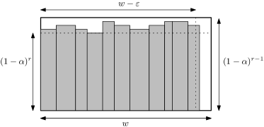
Figure 8: Shelf for narrow items of group $r$ (dense)

When the instance consists of narrow items only, the concept of shelf algorithms yields an online AFPTAS immediately. This is shown next in Section 4.1. However, the goal is to integrate narrow items into the container packing introduced in Section 2. We show in Section 4.2 how to fill gaps in the container packing with shelfs of narrow items. This first-fit-algorithm for narrow items maintains an asymptotic approximation ratio of $1+\mathcal{O}\left(\epsilon\right)$, as finally shown in Lemma 4.7.

4.1 Narrow Items Only

Consider the following first-fit shelf algorithm: Place an item of group $r$ into the first shelf of group $r$ where it fits. If there is no such shelf, open a new shelf of group $r$ on top of the packing.

Lemma 4.1.

The shelf algorithm with parameter $\alpha=\frac{\epsilon^{2}}{1-\epsilon^{2}}$ yields a packing of height at most $(1+\epsilon)\operatorname{OPT}(I_{N})+\mathcal{O}\left(1/\epsilon^{4}\right)$.

Proof.

Let $\beta_{r}$ the number of shelfs of group $r$ in the packing obtained by the shelf algorithm. Further, for a group $r$ let $I_{r}=\{i\in I\mid h(i)\in[(1-\alpha)^{r},(1-\alpha)^{r-1})\}$ . Each dense shelf for group $r$ contains items of size at least $(1-\alpha)^{r}(1-\epsilon)$, see Figure 8. Note that by the first-fit-principle, for each group at most one shelf is sparse. Thus there are at least $\beta_{r}-1$ dense shelfs for each group $r$, hence $\operatorname{SIZE}(I_{r})\geq(\beta_{r}-1)(1-\alpha)^{r}(1-\epsilon)$, or equivalently

$$\beta_{r}\leq\operatorname{SIZE}(I_{r})(1-\alpha)^{-r}(1-\epsilon)^{-1}+1\,.$$ (4.1)

The packing consists of $\beta_{r}$ shelfs of height $(1-\alpha)^{r-1}$ for each group $r$ (set $\beta_{r}=0$ if the group does not exist). Therefore, the packing height is by Equation 4.1

$$\sum_{r=0}^{\infty}\beta_{r}(1-\alpha)^{r-1}\leq\sum_{r=0}^{\infty}\left(\operatorname{SIZE}(I_{r})(1-\alpha)^{-r}(1-\epsilon)^{-1}+1\right)(1-\alpha)^{r-1}\,.$$

By splitting the sum and moving constant factors in front we get that the last term equals

$$\frac{1}{(1-\epsilon)(1-\alpha)}\sum_{r=0}^{\infty}\operatorname{SIZE}(I_{r})+\sum_{r=0}^{\infty}(1-\alpha)^{r-1}\leq(1+\epsilon)\operatorname{SIZE}(I_{N})+\sum_{r=0}^{\infty}(1-\alpha)^{r-1}\,,$$

where the inequality follows by definition of $\alpha$ and $I_{r}$. Since $\operatorname{SIZE}(I_{N})\leq\operatorname{OPT}(I_{N})$, the claim follows if we can show that the additive term is $\mathcal{O}\left(1/\epsilon^{4}\right)$. This follows by the geometric series: $\sum_{r=0}^{\infty}(1-\alpha)^{r-1}=\frac{1}{1-\alpha}\sum_{r=0}^{\infty}(1-\alpha)^{r}=\frac{1}{1-\alpha}\frac{1}{\alpha}=\mathcal{O}\left(1/\epsilon^{4}\right)$. ∎

4.2 Combination with Container Packing

As shown in Section 4.1 shelfs are a good way to pack narrow items efficiently. But before opening a new shelf that increases the packing height, we have to ensure that the existing packing is well-filled. Therefore, the idea is to fill gaps in the container packing with shelfs of narrow items. Thereby, we define a gap is the rectangle of height $h_{B}$ that fills the remaining width of an aligned level.

To simplify the following proofs, we introduce artificial D-containers filling the remaining width of a container level completely and think of placing shelfs inside the D-containers. We say that a D-container is full if shelfs of total height greater than $h_{B}-1$ are placed inside. For this section, we call the containers for big and flat items (introduced in Section 2) C-containers to distinguish them from D-containers that contain shelfs of narrow items.

A level is called well-filled if the total width of containers (including the D-container, if existing) is at least $1-2\epsilon$, and badly-filled otherwise. Figure 9(a) shows a container packing filled with D-containers: All levels are well-filled, assuming that the gray dashed area is of total width less than $2\epsilon$. Note that a badly-filled level can be made well-filled by aligning the C-containers with the Align operation and then define a D-container of the remaining width.

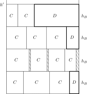
(a) Well-filled container packing

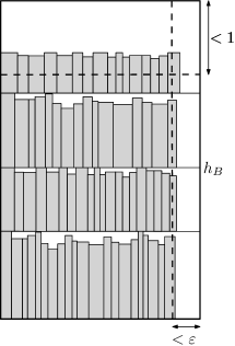
(b) Full D-container

Figure 9: D-containers are introduced to fill gaps in the container packing with shelfs.

Further, we introduce the term load: For a container-rectangle $r$, let $\operatorname{LOAD}(r)$ denote the total size of items that are packed inside the rectangle $r$. Clearly, $\operatorname{LOAD}(r)\leq\operatorname{SIZE}(r)$. For example, see the dense shelf $r$ for group $s$ in Figure 8: Here, $\operatorname{LOAD}(r)\geq(1-\alpha)^{s}(w-\epsilon)$. If $R$ is a set of rectangles, we define $\operatorname{LOAD}(R)=\sum_{r\in R}\operatorname{LOAD}(r)$.

In the following, we use $\alpha=\epsilon$ as shelf parameter and set $\lambda=1/(\epsilon-\epsilon^{2})$. Remember that the total height of sparse shelfs is at most $\sum_{r=0}^{\infty}(1-\epsilon)^{r-1}=1/(\epsilon-\epsilon^{2})=\lambda$ (see Section 4.1).

4.2.1 Insertion Algorithm

Similar to flat items, we need a buffer for narrow items. The N-Buffer is a rectangular segment of height $h_{B}$ and width 1 placed somewhere in the strip. Items inside the N-buffer are organized in shelfs.

First we define an auxiliary algorithm called Shelf-First-Fit. This algorithm tries to find a position for a narrow item without increasing the packing height. It may not use the N-buffer. If no such position exists, the algorithm returns $\mathit{false}$.

1

2

Input : Narrow item $i$ of group $r$

3

4if there is a shelf of group $r$ that can take $i$, place $i$ there

5 else if a new shelf of group $r$ can be opened without increasing the packing height, open it and place $i$ there

6 else return false

Algorithm 12 Shelf-First-Fit

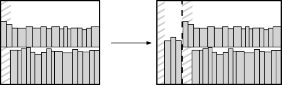
Figure 10: Placing a new shelf into the empty area of an enlarged D-container does not maintain the shelf structure in general.

With Algorithm 12 as a subroutine, we can give the entire algorithm for the insertion of narrow items in Algorithm 13. When an item can not be placed without increasing the packing height, the (full) N-buffer gets flushed: For this purpose, the algorithm tries to find $q$ badly-filled levels, where $q$ will be specified later. Aligning levels increases the area for shelfs, but the following observation is crucial:

Assume that a D-container is filled with shelfs and its width gets increased due to an Align operation. Placing a new shelf inside the new area does not maintain the shelf structure and thus not the lower bound on its load (see Figure 10 for an example). Therefore, when aligning a level, items in the respective D-container get temporarily removed. After aligning $q$ levels, removed items from former D-containers, the buffer items, and the current item get inserted via Shelf-First-Fit. This way, the shelf structure in the enlarged D-containers is maintained.

Finally, if there still remain items (for example, because there were too few badly-filled levels), new shelfs are opened on top of the packing. The next lemma states an important invariant property of Algorithm 13.

1

2

Input : Narrow item $i$

3

4if $i$ can be placed via Shelf-First-Fit or in the N-buffer, place $i$

5 else

      

       // N-Buffer is full. Align badly-filled levels

6       Let $L$ be the set of badly-filled levels

7       for $u\in L$, but at most $q$ times do

8             Align$(u)$

9             Remove items in D-container, if existing

10             Define empty D-container filling the remaining width

11            

12       end for

13      Empty N-buffer

14       Let $S$ be the set of all removed items from Lines 13 and 13, and item $i$

15       Try to reinsert each $j\in S$ via Shelf-First-Fit

16       For remaining items: Open new shelfs of width 1 on top of the packing

17      

Algorithm 13 Insertion of a narrow item

Lemma 4.2.

Algorithm 13 aligns at most $q=\mathcal{O}\left(1/\epsilon\right)$ levels and after repacking, the N-buffer is empty. Further, if it increases the packing height, all levels are well-filled and D-containers are full.

Proof.

For the first claim, note that the total size of $i$ and items from the N-buffer is at most $h_{B}+\epsilon$. We prove afterwards in Lemma 4.3 that $q=\mathcal{O}\left(1/\epsilon\right)$ is an appropriate choice. Afterwards in Line 13, the N-buffer is emptied. The last claim follows immediately from the description of the algorithm. ∎

Lemma 4.3.

In Algorithm 13, aligning $q=\mathcal{O}\left(1/\epsilon^{2}\right)$ levels is enough to (re-)insert items of size at most $h_{B}+\epsilon$.

Proof.

The crucial point is that narrow items of all aligned levels may also have to be reinserted. Let $W(D)$ be the total width of D-containers in $q$ aligned levels before aligning. The load of this D-containers is thus at most $W(D)h_{B}$. Therefore, narrow items of total size at most $h_{B}+\epsilon+W(D)h_{B}$ have to be (re-)inserted.

Next, we analyze the minimum load of a shelf packing in the enlarged D-containers. Let $D^{\prime}$ be the set of D-containers after aligning. We have $\left|{D^{\prime}}\right|=q$. Let $d^{\prime}\in D^{\prime}$ be the enlarged container to $d\in D$. Each D-container gets enlarged in width by at least $2\epsilon$, i. e. $w(d^{\prime})\geq w(d)+2\epsilon$ for all $d^{\prime}\in D$. For the load of a single D-container, we subtract $\epsilon$ from the width and 1 from the height, thus $\operatorname{LOAD}(d^{\prime})\geq(w(d^{\prime})-\epsilon)(1-\epsilon)(h_{B}-1)\geq(w(d)+\epsilon)(1-\epsilon)(h_{B}-1)$. The factor $1-\epsilon$ is due to height differences inside the groups. Thus, the total load of containers in $D^{\prime}$ is

$$\operatorname{LOAD}(D^{\prime})\geq\left(\sum_{d^{\prime}\in D^{\prime}}\operatorname{LOAD}(d^{\prime})\right)-\lambda\geq(1-\epsilon)(h_{B}-1)(W(D)+q\epsilon)-\lambda\,,$$

where the term $\lambda$ is due to sparse shelfs. In the remainder of the proof, we show

$$(1-\epsilon)(h_{B}-1)(W(D)+q\epsilon)-\lambda\geq h_{B}+\epsilon+W(D)h_{B}\,,$$ (4.2)

i. e. all items that have to be reinserted fit into the enlarged D-containers of the $q$ aligned levels. Note that no D-container in an aligned level has a width greater than $1-3\epsilon$, thus $W(D)\leq(1-3\epsilon)q$. Let $z=(1-\epsilon)(h_{B}-1)$ and $y=(1-3\epsilon)(z-h_{B})$. We show

$$(y+z\epsilon)q\geq h_{B}+\epsilon+\lambda\,,$$ (4.3)

which implies Equation (4.2), since Equation (4.2) is equivalent to $W(D)(z-h_{B})+zq\epsilon\geq h_{B}+\epsilon+\lambda$ and we have

$$W(D)(z-h_{B})+zq\epsilon =-W(D)(h_{B}-z)+zq\epsilon$$

$$\geq-(1-3\epsilon)q(h_{B}-z)+zq\epsilon W(D)\leq(1-3\epsilon)q$$

$$=(1-3\epsilon)q(z-h_{B})+zq\epsilon$$

$$=(y+z\epsilon)q$$

$$\geq h_{B}+\epsilon+\lambda eq.~\textup{(\ref{eq:enlargedDContainers2})}\,.$$

It holds that $y+z\epsilon\geq 12$ and with $q=2/\epsilon^{2}$ it follows that $(y+z\epsilon)q\geq 12q=24/\epsilon^{2}\geq 13/\epsilon^{2}+\epsilon+1/\epsilon^{2}\geq h_{B}+\epsilon+\lambda$, thus Equation (4.3) is shown. ∎

4.2.2 Analysis

The goal of this subsection is to show that if Algorithm 13 increases the packing height, the packing up to the previous height is well-filled. As the first step, we analyze the load of C-containers in the following lemma. The ideas in the proof are similar to those used in Section 2.3.

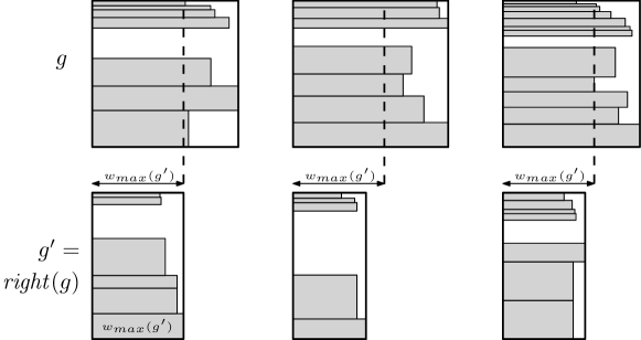
Figure 11: Containers of group $g$ have total load at least $h(g)w_{max}(g^{\prime})$.

Lemma 4.4.

Let $C_{\mathit{con}}$ be a container instance. Then, $\operatorname{LOAD}(C_{\mathit{con}})\geq(1-2\epsilon)\operatorname{SIZE}(C_{\mathit{con}})-\mathcal{O}\left(\omega/\epsilon^{3}\right)$.

Proof.

We write $C$ instead of $C_{\mathit{con}}$ for short. For a category $l\in W$, the group $g_{0}(l)$ is defined as $(l,A,0)$ if block $A$ is non-empty, and otherwise $(l,B,0)$. Let $G_{1}=G\setminus\bigcup_{l\in W}g_{0}(l)$. Further, let $g\in G_{1}$ and $g^{\prime}=\mathit{right}(g)$. With ($\mathcal{I}$3)- ($\mathcal{I}$4) we have $K_{g}\geq K_{g^{\prime}}$ (set $K_{g^{\prime}}=0$, if $g^{\prime}$ is not defined).

First, we consider the load of containers of the group $g$. Let $C(g)=\{c\in C\mid R(c)=g\}$ be the set of such containers. By ($\mathcal{I}$2), each container of group $g$ contains items of width at least $w_{max}(g^{\prime})$ (see Figure 11) and height $h(g)$. We have:

$$\operatorname{LOAD}(C(g)) \geq h(g)w_{max}(g^{\prime})$$ (4.4)

$$\geq(h_{B}-1)(K_{g}-1)w_{max}(g^{\prime}) \mathcal{I}$$ (5)

$$=(h_{B}K_{g}-h_{B}-K_{g}+1)w_{max}(g^{\prime})$$

$$=h_{B}K_{g}w_{max}(g^{\prime})-(h_{B}+K_{g}-1)w_{max}(g^{\prime})$$

$$\geq h_{B}K_{g^{\prime}}w_{max}(g^{\prime})-(h_{B}+K_{g}-1)w_{max}(g^{\prime}) K_{g}\geq K_{g^{\prime}}$$

$$\geq\operatorname{SIZE}(C(g^{\prime}))-(h_{B}+K_{g}-1) w_{max}(g^{\prime})\leq 1$$

Now consider the set of groups $G_{2}=G_{1}\setminus\bigcup_{l\in W}\mathit{right}(g_{0}(l))$ (i. e. we drop also the $(l,X,1)$-groups from $G$). Let $g^{\prime}=\mathit{right}(g)$ for all $g\in G_{1}$. Then, $\{g^{\prime}\mid g\in G_{1}\}=\{\mathit{right}(g)\mid g\in G_{1}\}=G_{2}$. Furthermore, let $C_{1}$, $C_{2}$ be the sets of container rectangles of groups $G_{1}$, $G_{2}$. Summing over each group in $G_{1}$ gives the total load of containers in $C_{1}$:

$$\operatorname{LOAD}(C_{1}) =\sum_{g\in G_{1}}\operatorname{LOAD}(C(g))$$

$$\geq\sum_{g\in G_{1}}\operatorname{SIZE}(C(g^{\prime}))-(h_{B}+K_{g}-1)$$ eq. (4.4)

$$=\sum_{g\in G_{2}}\operatorname{SIZE}(C(g))-\sum_{g\in G_{1}}h_{B}+K_{g}-1$$

$$\geq\operatorname{SIZE}(C_{2})-\left|{G_{1}}\right|(h_{B}+K_{g}^{*}-1)\,,$$

where $K_{g}^{*}=\max_{g\in G_{1}}K_{g}$. As the next step, we show $\left|{G_{1}}\right|(h_{B}+K_{g}^{*}-1)\leq\epsilon\operatorname{SIZE}(I_{L})+\mathcal{O}\left(\omega/\epsilon^{3}\right)$, implying

$$\operatorname{LOAD}(C_{1})\geq\operatorname{SIZE}(C_{2})-\epsilon\operatorname{SIZE}(I_{L})-\mathcal{O}\left(\omega/\epsilon^{3}\right)\,.$$ (4.5)

With ($\mathcal{I}$3)-($\mathcal{I}$4) we get $K_{g}^{*}\leq 2^{l}k\leq\frac{1}{\epsilon}k=\frac{1}{\epsilon}\left\lfloor{\frac{\epsilon}{4\omega h_{B}}\operatorname{SIZE}(I_{L})}\right\rfloor\leq\frac{1}{4\omega h_{B}}\operatorname{SIZE}(I_{L})\,.$ Since $G_{1}$ contains less than $\left|{G}\right|\leq\omega\left(2+\frac{16}{\epsilon}\right)$ groups (by Lemma 2.7), it follows that

$$\left|{G_{1}}\right|K_{g}^{*}\ \leq\omega\left(2+\frac{16}{\epsilon}\right)\frac{1}{4\omega h_{B}}\operatorname{SIZE}(I_{L})=\frac{2\epsilon+16}{4\epsilon h_{B}}\operatorname{SIZE}(I_{L})\leq\epsilon\operatorname{SIZE}(I_{L})\,.$$

Further, the term $\left|{G_{1}}\right|(h_{B}-1)$ is bounded by $\mathcal{O}\left(\omega/\epsilon^{3}\right)$, as $h_{B}\in\mathcal{O}\left(1/\epsilon^{2}\right)$. Thus, Equation (4.5) is shown. Like in the proof of Theorem 2.8 (Equation (2.8)), all containers of $(l,X,0)$-groups can be placed in $k$ levels of height $h_{B}$. Clearly, the same holds for $(l,X,1)$-groups and thus $\operatorname{SIZE}(C_{2})\geq\operatorname{SIZE}(C)-2\omega h_{B}k\geq\operatorname{SIZE}(C)-\epsilon\operatorname{SIZE}(I_{L})$. Using $\operatorname{LOAD}(C)\geq\operatorname{LOAD}(C_{1})$, Equation (4.5), and the last inequality with $\operatorname{SIZE}(I_{L})\leq\operatorname{SIZE}(C)$ completes the proof. ∎

The next lemma shows a similar result for D-containers.

Lemma 4.5.

Let $D$ be the set of all full D-containers in a packing of height $h^{\prime}$ (see Figure 9(a)). Assuming that in each D-container the loss of width is at most $2\epsilon$, it holds that $\operatorname{LOAD}(D)\geq(1-2\epsilon)\operatorname{SIZE}(D)-2\epsilon h^{\prime}-\lambda$.

Proof.

We first consider a single full D-container $d\in D$ like shown in Figure 9(b). The loss in height is at most 1 and the loss of width by assumption at most $2\epsilon$. Further, multiplying the height with factor $1-\epsilon$ regards height differences in the groups, thus:

$$\operatorname{LOAD}(d) \geq(1-\epsilon)(w(d)-2\epsilon)(h_{B}-1)$$

$$=(1-\epsilon)\left(w(d)h_{B}-w(d)-2\epsilon(h_{B}-1)\right)$$

$$\geq(1-\epsilon)w(d)h_{B}-w(d)-2\epsilon(h_{B}-1)\,.$$

Sparse shelfs can waste a total area of at most $\lambda$, therefore

$$\operatorname{LOAD}(D) =\left(\sum_{d\in D}\operatorname{LOAD}(d)\right)-\lambda$$

$$\geq\left(\sum_{d\in D}(1-\epsilon)w(d)h_{B}-w(d)-2\epsilon(h_{B}-1)\right)-\lambda$$

$$=(1-\epsilon)\operatorname{SIZE}(D)-\left(\sum_{d\in D}w(d)\right)-\left|{D}\right|2\epsilon(h_{B}-1)-\lambda$$

and with $$\sum_{d\in D}w(d)=\operatorname{SIZE}(D)\frac{1}{h_{B}}$$ it holds further

$$=\left(1-\epsilon-\frac{1}{h_{B}}\right)\operatorname{SIZE}(D)-2\left|{D}\right|\epsilon(h_{B}-1)-\lambda$$

$$\geq(1-2\epsilon)\operatorname{SIZE}(D)-2\epsilon h^{\prime}-\lambda\,,$$

where the last inequality follows from $1/{h_{B}}\leq\epsilon$ and $\left|{D}\right|\leq h^{\prime}/{h_{B}}$. ∎

The next corollary uses Lemmas 4.4 and 4.5 to bound the total load of a container packing filled with D-containers.

Corollary 4.6.

Let $C$ be a container instance and let a packing of $C$, filled with D-containers, of height $h^{\prime}$ be given. Let $I_{aux}$ be the set of all big, flat, and narrow items in the packing. If all levels are well-filled and all D-containers are full, then $\operatorname{SIZE}(I_{aux})\geq(1-4\epsilon)h^{\prime}-\mathcal{O}\left(\omega/\epsilon^{3}\right)$.

Proof.

According to Lemma 4.4, C-containers are filled with $\operatorname{LOAD}(C)\geq(1-2\epsilon)\operatorname{SIZE}(C)-z$ for $z=\mathcal{O}\left(\omega/\epsilon^{3}\right)$. For the sake of simplicity, we can assume that each level is aligned and that the remainder is filled by a D-container: The load is the same as if the level would be aligned and filled by an empty D-container. An unaligned but well-filled level has gaps of total width at most $2\epsilon$. Hence, the D-container would have a loss of width of at most $2\epsilon$ and we can apply Lemma 4.5.

As $h^{\prime}$ is the packing height and also the total area of the packing (in a strip of width 1), $\operatorname{SIZE}(D)=h^{\prime}-\operatorname{SIZE}(C)$ and it holds further

$$\operatorname{SIZE}(I_{aux}) =\operatorname{LOAD}(C)+\operatorname{LOAD}(D)$$

$$\geq(1-2\epsilon)\operatorname{SIZE}(C)-z+(1-2\epsilon)\operatorname{SIZE}(D)-2\epsilon h^{\prime}-\lambda$$

$$=(1-2\epsilon)\operatorname{SIZE}(C)+(1-2\epsilon)(h^{\prime}-\operatorname{SIZE}(C))-2\epsilon h^{\prime}-z-\lambda$$

$$=(1-4\epsilon)h^{\prime}-z-\lambda\,.$$

Since both terms $z$ and $\lambda$ are dominated by $\mathcal{O}\left(\omega/\epsilon^{3}\right)$, the claim is proven. ∎

Recall that Algorithm 13 only increases the packing height if all levels are well-filled and all D-containers are full, thus we obtain the following result. The main argument and the notation of Lemma 4.7 is similar to [21].

Lemma 4.7.

Let $h^{\prime}$ be the height of the container packing. Algorithm 13 returns a packing of height $h_{\mathit{final}}$, such that $h_{\mathit{final}}\leq\max\left\{h^{\prime},(1+\epsilon^{\prime})\operatorname{SIZE}(I)+\mathcal{O}\left(\omega/\epsilon^{3}\right)\right\}$, where $\epsilon^{\prime}\in\mathcal{O}\left(\epsilon\right)$.

Proof.

If Algorithm 13 does not reach Line 13, $h_{final}=h^{\prime}$ and thus the claim holds trivially. Now suppose that Algorithm 13 opens at least one new shelf in Line 13 placed on top of the packing. By Lemma 4.2, all levels are well-filled and all D-containers are full, and thus we can apply Corollary 4.6. Each horizontal segment in the packing is of one of two types: Either it is a container-level of height $h_{B}$ (containing C- and D-containers) or a shelf of width 1 (containing narrow items). Let $h^{\prime}$ be the total height of container-levels and $h^{\prime\prime}$ the total height of shelfs of width 1. Hence, $h_{final}=h^{\prime}+h^{\prime\prime}$. We partition the set of items $I$ into $I_{aux}$ like in Corollary 4.6 and ${I_{N}}^{\prime}$, the set of narrow items placed in shelfs of width 1. Let $\epsilon^{\prime}=\frac{1}{1-4\epsilon}-1\in\mathcal{O}\left(\epsilon\right)$ and $z=(1+\epsilon^{\prime})\mathcal{O}\left(\omega/\epsilon^{3}\right)$. Then, the conclusion of Corollary 4.6 is equivalent to:

$$h^{\prime}\leq(1+\epsilon^{\prime})\operatorname{SIZE}(I_{aux})+z$$ (4.6)

Further, with Lemma 4.1 we can bound the packing height for the shelfs of width 1. Remember that the N-buffer causes additional height of $h_{B}$. If we see it as part of the shelf packing, we get from the proof of Lemma 4.1 with $\alpha=\epsilon$:

$$h^{\prime\prime}\leq\frac{1}{(1-\epsilon)^{2}}\operatorname{SIZE}({I_{N}}^{\prime})+\lambda+h_{B}$$ (4.7)

The final packing height $h_{final}$ can be bounded as follows:

$$h_{\mathit{final}} =h^{\prime}+h^{\prime\prime}$$

$$\leq(1+\epsilon^{\prime})\operatorname{SIZE}(I_{aux})+z+\frac{1}{(1-\epsilon)^{2}}\operatorname{SIZE}({I_{N}}^{\prime})+\lambda+h_{B}$$ eq. (4.6),(4.7)

$$\leq(1+\epsilon^{\prime})\operatorname{SIZE}(I_{aux})+(1+\epsilon^{\prime})\operatorname{SIZE}({I_{N}}^{\prime})+\lambda+h_{B}+z$$

$$=(1+\epsilon^{\prime})\operatorname{SIZE}(I)+\lambda+h_{B}+z I=I_{aux}\mathbin{\dot{\cup}}{I_{N}}^{\prime}$$

Again, the additive terms $\lambda$, $h_{B}$, and $z$ are bounded by $\mathcal{O}\left(\omega/\epsilon^{3}\right)$. ∎

4.3 Changes in the Container Packing

So far we assumed a static layout of D-containers. But as the width of C-containers may change due to inserted or removed items, D-containers also change in width. Moreover, when the pattern (see LP 2.4) of a level changes, D-containers have to be redefined. In both cases, narrow items may have to be reinserted. This two scenarios are considered in the following.

4.3.1 Stretch Operation and Narrow Items

The Stretch operation (introduced in Section 3.1) changes the position of containers in one level such that no item overlaps with a C-container. When the stretched level includes a D-container, this may overfill a level (see the example in Figure 12). In the worst case, all items from a maximal filled D-container have to repacked, i. e. items of total size $(1-\epsilon)h_{B}$. Lemma 4.3 bounds the repacking size with $qh_{B}$ in this case.

(a) Before Stretch

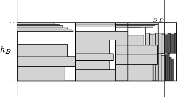
(b) After Stretch

Figure 12: Overlapping items (dark colored) after Stretch operation

4.3.2 Repacking of Levels

Recall that Algorithm 2 makes use of the operation Improve, which changes some components in the LP/ILP-solutions that represent the level configuration. In the packing several levels are repacked, which requires that the D-containers have to be rebuilt. The new set of D-containers may have a lower load since the widths change and thus sparse shelfs can occur. The next lemma bounds the total area of narrow items that may have to be packed outside the new D-containers.

Lemma 4.8.

Assume that the packing of C-containers changes in $p$ levels. Let $D$ be the set of D-containers in this levels before repacking and $D^{\prime}$ the set of new defined D-containers in the repacked and aligned levels. Then, $\operatorname{LOAD}(D)-\operatorname{LOAD}(D^{\prime})\leq\mathcal{O}\left(p/\epsilon\right)+~{}\lambda$.

Proof.

The proof is similar to the one of Lemma 4.3. Let $W(D)$ be the total width of the containers in $D$. Clearly, $\operatorname{LOAD}(D)\leq h_{B}W(D)$. The total area of the new containers in $D^{\prime}$ does not decrease in comparison to $D$, but the new defined shelfs can have a smaller load. An analog argument like in the proof of Lemma 4.3 gives $\operatorname{LOAD}(D^{\prime})\geq(1-\epsilon)(h_{B}-1)(W(D)-p\epsilon)-\lambda$. Since each D-container has width at most $1-\epsilon<1$, it holds that $W(D)<p$. Thus:

$$\operatorname{LOAD}(D)-\operatorname{LOAD}(D^{\prime})$$

$$\leq h_{B}W(D)-(1-\epsilon)(h_{B}-1)(W(D)-p\epsilon)+\lambda$$

$$=h_{B}W(D)-(1-\epsilon)(h_{B}-1)W(D)+(1-\epsilon)(h_{B}-1)p\epsilon+\lambda$$

$$=W(D)(h_{B}-(h_{B}-1-\epsilon h_{B}+\epsilon))+(1-\epsilon)(h_{B}-1)p\epsilon+\lambda$$

$$<W(D)(1+\epsilon h_{B})+p\epsilon+\lambda$$

$$=p(1+\epsilon h_{B}+\epsilon)+\lambda$$

The claim follows by $1+\epsilon h_{B}+\epsilon=\mathcal{O}\left(\epsilon h_{B}\right)=\mathcal{O}\left(1/\epsilon\right)$. ∎

4.4 Overall Algorithm

So far we presented online algorithms for the case where only narrow items are present (Section 4.1) and an algorithm that fills gaps in the container packing with narrow items (Algorithm 13). Recall that the container packing approach requires a minimum size of $I_{L}$.

Therefore, it remains to show how to handle the general setting, where narrow items arrive, while $\operatorname{SIZE}(I_{L}(t))$ is possibly too small for the container packing. For this purpose, the overall Algorithm 14 works in one of two modes: In the semi-online mode, small instances of $I_{L}$ are packed offline and arbitrary large instances of $I_{N}$ online. In contrast, in the online mode, the techniques of Sections 2 to 4 are applied.

Figure 13: Top-level sketch of the packing in the semi-online mode

Semi-online mode

The top-level structure of the packing in the semi-online mode is shown in Figure 13. It is divided into three parts:

• To avoid that flat items cause a huge amount of repacking, we use an F-buffer for flat items like introduced in Section 3.5.3, but with slot height $y=2+\epsilon$.

• When the F-buffer overflows or a new big item arrives, a new packing of $I_{L}(t)$, including all items from the F-buffer, is obtained by the algorithm of Kenyon and Rémila (K&R) [21]. In the strip, we reserve a segment of fixed height $H$ for the changing packings of $I_{L}(t)$, where $H$ is the packing height of a maximum instance of $I_{L}(t)$.

• Narrow items are packed separately on top of the packing via the shelf algorithm described in Section 4.1.

Online mode

As soon as $\operatorname{SIZE}(I_{L}(t))\geq\frac{4\omega h_{B}}{\epsilon}(h_{B}+1)$, we go over to use Algorithms 8, 10, and 13, depending on the item type.

1

2

Input : Item $i_{t}$

3

4if $\operatorname{SIZE}(I_{L}(t))<\frac{4\omega h_{B}}{\epsilon}(h_{B}+1)$ then // Semi-online mode

5       if $i_{t}$ is flat then

6             Place $i_{t}$ in the F-buffer.

7            

8       if $i_{t}$ is big or F-buffer overflows then

9             Pack $I_{L}(t)$ (incl. items in the F-buffer and $i_{t}$) with K&R

10             Replace packing of $I_{L}(t-1)$ with the new packing

11      

12      if $i_{t}$ is narrow then

13             Place $i_{t}$ via shelf packing

14      

15 else  // Online mode

16       Use Algorithms 8, 10 or 13 depending on the type of $i_{t}$.

Algorithm 14 Insertion of an item in the general setting

The following theorem states that the overall Algorithm 14 returns a packing of the desired packing height.

Theorem 4.9.

Let $h$ be the height of the packing returned by Algorithm 14. It holds that $h\leq(1+\mathcal{O}\left(\epsilon\right))\operatorname{OPT}(I)\allowbreak+\mathrm{poly}(1/\epsilon)$.

Proof.

In the semi-online mode, the packing consists of two segments of constant height $\omega y=\mathcal{O}\left(\log\frac{1}{\epsilon}\right)$ and $H=\mathcal{O}\left(\frac{\omega{h_{B}}^{2}}{\epsilon}\right)$ (see Figure 13) and the shelf packing of height $h^{\prime}$. By Lemma 4.1, $h^{\prime}\leq(1+\epsilon)\operatorname{OPT}(I_{N})+\mathcal{O}\left(1/\epsilon^{4}\right)$. Therefore, the total packing height is at most $(1+\epsilon)\operatorname{OPT}(I_{N})+\mathcal{O}\left(1/\epsilon^{4}\right)+\mathcal{O}\left(\log\frac{1}{\epsilon}\right)+\mathcal{O}\left(\frac{\omega{h_{B}}^{2}}{\epsilon}\right)\leq(1+\epsilon)\operatorname{OPT}(I)+\mathrm{poly}(1/\epsilon)$.

In the online mode, Lemma 4.7 bounds the final packing height after insertion of narrow items with $h_{\mathit{final}}\leq\max\left\{h^{\prime},(1+\epsilon^{\prime})\operatorname{SIZE}(I)+\mathcal{O}\left(\omega/\epsilon^{3}\right)\right\}$, where $h^{\prime}$ is the height of the container packing and $\epsilon^{\prime}\in\mathcal{O}\left(\epsilon\right)$. In the case $h_{final}=h^{\prime}$, we need the result from Theorem 3.12. Equation (3.9) states $h^{\prime}\leq(1+2\Delta)\operatorname{OPT}(I_{L})+2(1+\epsilon)z+m$, where $\Delta=\mathcal{O}\left(\epsilon\right)$, $z=\mathcal{O}\left(1/\epsilon^{2}\right)$, and $m=\mathcal{O}\left(\frac{1}{\epsilon}\log\frac{1}{\epsilon}\right)$. With $\operatorname{OPT}(I_{L})\leq\operatorname{OPT}(I)$, the claim follows. In the other case $h_{final}>h^{\prime}$, the claim follows directly by $\operatorname{SIZE}(I)\leq\operatorname{OPT}(I)$ and $\omega=\mathcal{O}\left(\frac{1}{\epsilon}\log\frac{1}{\epsilon}\right)$. ∎

5 Migration Analysis

Let $\mathrm{Repack}(t)$ denote the total size of repacked items at time $t\geq 1$, i. e. at the arrival of item $i_{t}$. Recall out notion of amortized migration: While in [24] for the migration factor $\mu$ holds $\mathrm{Repack}(t)\leq\mu\operatorname{SIZE}(i_{t})$, we say that an algorithm has amortized migration factor $\mu$ if $\sum_{j=1}^{t}\mathrm{Repack}(j)\leq\mu\operatorname{SIZE}(I(t))$, where $I(t)=\{i_{1},\ldots,i_{t}\}$. A useful interpretation of amortized migration is the notion of repacking potential, also used by Skutella and Verschae in [26]. Each arriving item $i_{t}$ charges a global repacking budget with its repacking potential $\mu\operatorname{SIZE}(i_{t})$. Repacking a set of items $R$ costs $\operatorname{SIZE}(R)$ and is paid from the budget.

If we waant to show that $\mu$ is the amortized migration factor, it suffices to show that the budget is non-negative at each time:

Lemma 5.1.

Let $\Phi(t)$ denote the repacking budget at time $t$ and assume $\Phi(0)=0$. If $\Phi(t)\geq 0$ at each time $t\geq 1$, it holds that $\sum_{j=1}^{t}\mathrm{Repack}(j)\leq\mu\operatorname{SIZE}(I(t))$.

The proof of Lemma 5.1 follows by a standard argument for potential functions, see [7, Sec. 17.3].

5.1 Repacking of Operations

As the first step we consider the repacking performed by the two major operations Shift and ShiftA used for the insertion of a big or flat item. In the following analysis we use the values $\omega,d,q,h_{B},p$ as defined in previous chapters. See Table 1 for a summary.

5.1.1 Shift

In general, shifting an item $i_{t}$ into a group is followed by a sequence of shift operations and thus the repacking performed in each shift operation sums up to the total repacking. The maximum amount of repacking occurs in a sequence beginning in group $(l,B,q(l,B))$ and ending in group $(l,A,-1)$. Therefore, we consider the sequence of shift operations

$$\textsc{Shift}(g^{0},S^{0}),\textsc{Shift}(g^{1},S^{1}),\ldots,\textsc{Shift}(g^{d-1},S^{d-1}),\textsc{Shift}(g^{d},S^{d})$$

with $S^{0}=\{i_{t}\}$, $g^{0}=(l,B,q(l,B))$, $g^{d-1}=(l,A,0)$, and $g^{d}=(l,A,-1)$. See Figure 14. Like in Section 3.2.1, let $S^{j}$ and $S_{out}^{j}$ be the sets $S$, $S_{out}$ for the call Shift$(g^{j},S^{j})$. For the maximum amount of repacking we can assume

$$h(S^{j})=h(S_{out}^{j-1})\leq h(S_{out}^{j})\,.$$ (5.1)

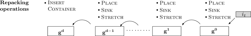
Figure 14: Repacking in a maximum shift sequence

Lemma 5.2.

The total repacking in the above defined shift sequence is at most $\mathcal{O}\left(\frac{qh_{B}d^{2}}{\epsilon}\right)$.

Proof.

Repacking in the Shift operation (Algorithm 3) is performed by the auxiliary operations Sink, Place, Stretch, and InsertContainer. Note that the repacking of the first three operations depends on their position in the shift sequence. An operation is at position $j$ if it is performed as part of Shift$(g^{j},S^{j})$. First we analyze the repacking of the operations Sink, Place, Stretch at position $j$ with $0\leq j\leq d$.

Sink

The Sink operation is necessary for each container that contains a big item from $S_{out}^{j}$. Since each big item has minimum height $\epsilon$, the number of big items in $S_{out}^{j}$ is at most $\left\lfloor{h(S_{out}^{j})/\epsilon}\right\rfloor$. Hence, the same bound holds for the number of affected containers. Flat items in $S_{out}^{j}$ do not cause sinking (see Section 3.5.3). The repacking for each sinked container is at most $h_{B}$, thus we get

$$\mathit{Repack\_Sink}(j)\leq\left\lfloor{\frac{h(S_{out}^{j})}{\epsilon}}\right\rfloor h_{B}\leq h(S_{out}^{j})\frac{h_{B}}{\epsilon}\,.$$ (5.2)

Place (without Stretch)

Remember that the placing differs depending on the item type: Big items get placed via Algorithm 9 without repacking, while placing flat items via Algorithm 11 requires resorting of containers. For a worst-case analysis we assume $S^{j}$ to consist of flat items solely. When placing the set $S^{j}$ with Algorithm 11, the repacking size is at most $nh_{B}$, where $n$ is the size of the partition in Line 10. A partition into at most $\left\lceil{h(S^{j})/(1-\epsilon)}\right\rceil+1$ sets can be found greedily. Using Equation (5.1) gives

$$\mathit{Repack\_Place}(j)\leq\left(\left\lceil{\frac{h(S^{j})}{1-\epsilon}}\right\rceil+1\right)h_{B}\leq h(S_{out}^{j})\frac{h_{B}}{1-\epsilon}+2h_{B}\,.$$ (5.3)

Stretch

First, we bound the number of containers where items from $S^{j}$ could be placed. Let $S^{j}$ be partitioned into $S^{j}_{b}$ and $S^{j}_{f}$, the sets of big and flat items. Items from $S^{j}_{b}$ can be placed in at most $\left\lfloor{h(S^{j}_{b})/\epsilon}\right\rfloor$ containers since each big item as minimum height $\epsilon$. As analyzed in the previous paragraph, flat items get placed in at most $\frac{h(S^{j}_{f})}{1-\epsilon}+2$ containers. With Equation (5.1) we get

$$\left\lfloor{\frac{h(S^{j}_{b})}{\epsilon}}\right\rfloor+\frac{h(S^{j}_{f})}{1-\epsilon}+2\leq\frac{h(S^{j}_{b})}{\epsilon}+\frac{h(S^{j}_{f})}{\epsilon}+2=\frac{h(S^{j})}{\epsilon}+2\leq\frac{h(S_{out}^{j})}{\epsilon}+2$$

as the total number of containers where new items may be placed. Each placing in a container is followed by a Stretch operation, which repacks containers of one level. In addition, a D-container with narrow items has to be repacked. Using the result from Lemma 4.3, the repacking for one stretched level is bounded by $h_{B}+qh_{B}=\mathcal{O}\left(qh_{B}\right)$.

$$\mathit{Repack\_Stretch}(j) \leq\left(\frac{h(S_{out}^{j})}{\epsilon}+2\right)\mathcal{O}\left(qh_{B}\right)=h(S_{out}^{j})\cdot\mathcal{O}\left(\frac{qh_{B}}{\epsilon}\right)+\mathcal{O}\left(qh_{B}\right)$$ (5.4)

InsertContainer

Corollary 3.3 states that the total height of items that have to be packed into new containers is at most $h(S^{0})+h_{B}-2\leq h_{B}-1$. Therefore, exactly one container gets inserted. The insertion of a container via Algorithm 2 makes use of Improve, which repacks $p$ levels. In addition, according to Lemma 4.8, narrow items of maximum size $\mathcal{O}\left(p/\epsilon\right)+\lambda$ have to be reinserted. With Lemma 4.3, at most $\frac{\mathcal{O}\left(p/\epsilon\right)+\lambda}{h_{B}+\epsilon}=\mathcal{O}\left(\frac{p}{\epsilon h_{B}}\right)$ times $q$ levels get aligned. Using $h_{B}=\mathcal{O}\left(q\right)$ gives:

$$\mathit{Repack\_InsCon}\leq ph_{B}+\mathcal{O}\left(\frac{p}{\epsilon h_{B}}\right)qh_{B}=\mathcal{O}\left(pq\right)+\mathcal{O}\left(\frac{pq}{\epsilon}\right)=\mathcal{O}\left(\frac{pq}{\epsilon}\right)$$ (5.5)

Conclusion

Sinking, placing, and stretching occurs in the first $d$ of the $d+1$ shift steps. With Equations (5.2) to (5.4) , this repacking is at most of size:

$$\quad\sum_{j=0}^{d-1}\mathit{Repack\_Sink}(j)+\mathit{Repack\_Place}(j)+\mathit{Repack\_Stretch}(j)$$ (5.6)

$$\leq\sum_{j=0}^{d-1}\left(h(S_{out}^{j})\frac{h_{B}}{\epsilon}\right)+\left(h(S_{out}^{j})\frac{h_{B}}{1-\epsilon}+2h_{B}\right)+\left(h(S_{out}^{j})\cdot\mathcal{O}\left(\frac{qh_{B}}{\epsilon}\right)+\mathcal{O}\left(qh_{B}\right)\right)$$

$$=\left(\frac{h_{B}}{\epsilon}+\frac{h_{B}}{1-\epsilon}+\mathcal{O}\left(\frac{qh_{B}}{\epsilon}\right)\right)\left(\sum_{j=0}^{d-1}h(S_{out}^{j})\right)+d\left(2h_{B}+\mathcal{O}\left(qh_{B}\right)\right)$$

$$=\mathcal{O}\left(\frac{qh_{B}}{\epsilon}\right)\left(\sum_{j=0}^{d-1}h(S_{out}^{j})\right)+d\cdot\mathcal{O}\left(qh_{B}\right)$$

$$\overset{(*)}{=}\mathcal{O}\left(\frac{qh_{B}d^{2}}{\epsilon}\right)+\mathcal{O}\left(dqh_{B}\right)$$

$$=\mathcal{O}\left(\frac{qh_{B}d^{2}}{\epsilon}\right)$$

where ($*$) holds since $h(S_{out}^{j})\leq j+3+\epsilon$ for $h(S^{0})=h(i_{t})\leq 1$ (Lemma 3.2) and with the Gauss sum $\sum_{j=0}^{d-1}h(S_{out}^{j})\leq\sum_{j=0}^{d-1}j+3+\epsilon\leq\sum_{j=0}^{d-1}\mathcal{O}\left(j\right)=\mathcal{O}\left(d^{2}\right)$ follows.

Additionally, the repacking due to InsertContainer is by Equation (5.5) at most $\mathcal{O}\left(\frac{pq}{\epsilon}\right)$. As $p=\mathcal{O}\left(d^{2}\right)$ (see Table 1), the first three operations dominate the total repacking. ∎

Table 1: Variables used for the migration analysis

Symbol	Meaning	Asymptotic bound	Reference
$\omega$	# categories	$\mathcal{O}\left(\log\frac{1}{\epsilon}\right)$	Lemma 2.7
$d$	max. length of shift sequence	$\mathcal{O}\left(\frac{1}{\epsilon}\log\frac{1}{\epsilon}\right)$	Lemma 2.7
$q$	# aligned levels in Algorithm 13	$\mathcal{O}\left(1/\epsilon^{2}\right)$	Lemma 4.3
$h_{B}$	container height	$\mathcal{O}\left(1/\epsilon^{2}\right)$	Section 2.3
$p$	# repacked levels by Improve	$\mathcal{O}\left(\frac{1}{\epsilon^{2}}\log\frac{1}{\epsilon}\right)$	Theorem 3.11

5.1.2 ShiftA

The steps performed in Lines 4-4 of Algorithm 4 (ShiftA) are analog to Lines 3-3 of Algorithm 3 (Shift), except for the height of the shifted items. Therefore, we reduce these parts of ShiftA to Shift, in order to make use of Equations (5.2) to (5.4) .

Lemma 5.3.

The total repacking performed in one call of Algorithm 4 is at most $\mathcal{O}\left(\frac{q{h_{B}}^{2}\omega}{\epsilon^{2}}\right)$.

Proof.

After the for-loop in Algorithm 4, there are three more sources of repacking: First, the $2^{l}$ new containers get inserted with Algorithm 5. Then, some items of group $(l,B,q(l,B))$ might be moved to other containers within the group. Finally, some containers may get deleted by Algorithm 6. First, we consider the steps analog to Shift.

Sink, Place, Stretch

Let $b=q(l,B)$. For each iteration $j\leq b$ of the for-loop in Algorithm 4, let $S^{j}$ be the set $S$ defined in Line 4. Repacking operations are sinking the containers with items from $S^{j}$ (in group $g_{j+1}$), placing $S^{j}$ (in group $g_{j}$) and stretching of levels affected by the placing of $S^{j}$. Therefore, we can apply Equations (5.2) to (5.4) if we set $S_{out}^{j}=S^{j}$. With the definition of $u$ in Line 4 of Algorithm 4 we get

$$h(S^{0})\leq s_{min}+1=u-h(g_{0})\overset{\text{\ref{inv:e:heightInterval}}}{\leq}2^{l}k(h_{B}-1)-((2^{l}(k-1)-1)(h_{B}-1)\\ =(2^{l}+1)(h_{B}-1)$$

and for $1\leq j<b$

$$h(S^{j})\leq s_{min}+1=u-h(g_{0})\overset{\text{\ref{inv:e:heightInterval}}}{\leq}2^{l}(k-1)(h_{B}-1)-((2^{l}(k-1)-1)(h_{B}-1)\\ =h_{B}-1\,.$$

Since $b\leq q(l,A)+q(l,B)=\mathcal{O}\left(\frac{\omega}{\epsilon}\right)$ (by Lemma 2.7), it follows $2^{l}+b=\mathcal{O}\left(\frac{\omega}{\epsilon}\right)$, and thus $\sum_{j=0}^{b-1}h(S^{j})\leq(2^{l}+1)(h_{B}-1)+(b-1)(h_{B}-1)=(2^{l}+b)(h_{B}-1)=\mathcal{O}\left(\frac{\omega h_{B}}{\epsilon}\right)\,.$ Analogously to Lemma 5.2 we get

$$\quad\sum_{j=0}^{b-1}\mathit{Repack\_Sink}(j)+\mathit{Repack\_Place}(j)+\mathit{Repack\_Stretch}(j)$$ (5.7)

$$=\mathcal{O}\left(\frac{qh_{B}}{\epsilon}\right)\left(\sum_{j=0}^{b-1}h(S^{j})\right)+\mathcal{O}\left(bqh_{B}\right)~{}~{}=\mathcal{O}\left(\frac{q{h_{B}}^{2}\omega}{\epsilon^{2}}\right)\,.$$

Repacking of $q(l,B)$

At most $\lceil{\frac{\Delta}{h_{B}-1}}\rceil$ containers have to be emptied and by Equation (3.2) this term is at most $\lceil{2^{l}+1}\rceil$. Therefore,

$$\mathit{Repack\_{EmptyCon}}\leq\left\lceil{2^{l}+1}\right\rceil h_{B}=\mathcal{O}\left(\frac{h_{B}}{\epsilon}\right)\,.$$ (5.8)

Insert / Delete Containers

Algorithm 5 needs one call of Improve, analogously to the proof for Shift (Equation (5.5)) the size of repacking is at most $\mathcal{O}\left(\frac{pq}{\epsilon}\right)$. Before containers get deleted, contained items are repacked into other containers, which is already treated above. There are at most $\lceil{2^{l}+1}\rceil$ containers that may get deleted (see above), each of them requires a single call of Algorithm 6.

$$\mathit{Repack\_InsDelCon}\leq\mathcal{O}\left(\frac{pq}{\epsilon}\right)\left\lceil{2^{l}+1}\right\rceil=\mathcal{O}\left(\frac{pq}{\epsilon^{2}}\right)\,.$$ (5.9)

Conclusion

Using Equations (5.7) to (5.9) , we notice that the operations Sink, Place, and Stretch dominate the overall repacking:

$$\mathcal{O}\left(\frac{q{h_{B}}^{2}\omega}{\epsilon^{2}}\right)+\mathcal{O}\left(\frac{h_{B}}{\epsilon}\right)+\mathcal{O}\left(\frac{pq}{\epsilon^{2}}\right)=\mathcal{O}\left(\frac{q{h_{B}}^{2}\omega}{\epsilon^{2}}\right)\,.$$

∎

5.2 Putting it together

Now we are able to analyze the amortized migration factor of the presented algorithm. Let $i_{t}$ be the item inserted at time $t\geq 1$. For the amortized analysis we use the notion of repacking potential, thus let $\Phi(t)=\Phi(t-1)+\mu\operatorname{SIZE}(i_{t})-\mathrm{Repack}(t)$ be the total budget at time $t$ and assume $\Phi(0)=0$.

5.2.1 Insertion of a Big or Flat Item

Let $\varGamma$ be the maximum total size of repacking in a shift sequence. By Lemma 5.2, $\varGamma=\mathcal{O}\left(\frac{qh_{B}d^{2}}{\epsilon}\right)$. First we need the following result, regarding the amount of repacking caused by the block balancing algorithm:

Lemma 5.4.

The block balancing procedure (Algorithm 7) for a set of items $M$ causes repacking of size at most $\mathcal{O}\left(\frac{q{h_{B}}\omega}{\epsilon^{2}}\right)\operatorname{SIZE}(M)$.

Proof.

Lemma 3.8 states that the total number of moved groups for the insertion of $M$ is at most $\frac{8+\epsilon}{2h_{B}}\operatorname{SIZE}(M)+1$. According to Lemma 5.3, moving one single group via ShiftA causes repacking of size $\mathcal{O}\left(\frac{q{h_{B}}^{2}\omega}{\epsilon^{2}}\right)$. That is, the total repacking is at most $\mathcal{O}\left(\frac{q{h_{B}}^{2}\omega}{\epsilon^{2}}\right)\left(\frac{8+\epsilon}{2h_{B}}\operatorname{SIZE}(M)+1\right)\allowbreak=\mathcal{O}\left(\frac{q{h_{B}}\omega}{\epsilon^{2}}\right)\operatorname{SIZE}(M)$. ∎

Since big items have a minimum size we immediately get the following result even without amortization:

Lemma 5.5.

Inserting a big item via Algorithm 8 has migration factor $\mu=\mathcal{O}\left(\frac{qh_{B}d^{2}}{\epsilon^{3}}\right)$.

Proof.

The first repacking source in Algorithm 8 is Shift, whose repacking size is at most $\varGamma$. Additionally, the block balancing (Algorithm 7) causes repacking. Considering a single big item $i_{t}$, Lemma 5.4 with $M=\{i_{t}\}$ bounds the repacking size with $\mathcal{O}\left(\frac{q{h_{B}}\omega}{\epsilon^{2}}\right)$. Since this term is dominated by $\varGamma$, the total repacking in Algorithm 8 is $\mathcal{O}\left(\varGamma\right)$. Each big item has minimum size $\epsilon^{2}$, thus $\mu=\frac{\mathcal{O}\left(\varGamma\right)}{\epsilon^{2}}=\mathcal{O}\left(\frac{qh_{B}d^{2}}{\epsilon^{3}}\right)$. ∎

The insertion of a flat item is closely related to the procedure for big items. But since flat items get buffered before the Shift operation, here the amortized analysis comes into play.

Lemma 5.6.

Inserting a flat item via Algorithm 10 has amortized migration factor $\mu=\mathcal{O}\left(\frac{qh_{B}d^{2}}{\epsilon^{4}}\right)$.

Proof.

Let $i_{t}$ be the inserted item of category $l$ and let $\mu=\mathcal{O}\left(\frac{1}{\epsilon^{3}}\right)\varGamma$. If $i_{t}$ can be inserted without overflowing the F-buffer, no repacking is performed. Now suppose that an overflow occurs. Then, each of the $2^{l}$ slots contains items of width at least $2^{-(l+1)}$ and total height at least $y-\epsilon=\left|{G}\right|\epsilon^{2}$. Consequently, all slots of category $l$ contain items of total size at least $2^{l}2^{-(l-1)}\left|{G}\right|\epsilon^{2}=\frac{1}{2}\left|{G}\right|\epsilon^{2}$. None of those items used its repacking potential so far, thus $\Phi(t-1)\geq\mu\frac{1}{2}\left|{G}\right|\epsilon^{2}=\mathcal{O}\left(1/\epsilon\right)\left|{G}\right|\varGamma$.

The repacking in Algorithm 10 is due to Shift, which is called $\left|{G(l)}\right|n$ times, where $\left|{G(l)}\right|\leq\left|{G}\right|$ denotes the number of groups of category $l$ and $n$ the size of the partition (see Line 10). By Lemma 3.9, $n\leq\mathcal{O}\left(1/\epsilon\right)$. Like in the case of big items (Lemma 5.5), the repacking of ShiftA is dominated by the repacking for Shift. Hence, $\mathrm{Repack}(t)\leq\mathcal{O}\left(1/\epsilon\right)\left|{G}\right|\varGamma$ and $\Phi(t)\geq 0$.

∎

5.2.2 Insertion of a Narrow Item

Lemma 5.7.

The insertion of a narrow item with Algorithm 13 has amortized migration factor $\mu=\mathcal{O}\left(q\right)=\mathcal{O}\left(1/\epsilon^{2}\right)$.

Proof.

Let $\mu=\frac{(q+1)h_{B}}{(1-\epsilon)^{2}(h_{B}-1-\lambda)}$. If $i_{t}$ can be placed in the N-buffer or via Shelf-First-Fit, no repacking is performed. Now assume that $i_{t}$ can not be placed in the N-buffer. Recall that the N-buffer has width 1 and height $h_{B}$, where sparse shelfs have total height at most $\lambda$. Thus, a full N-buffer contains items of total size at least $(1-\epsilon)^{2}(h_{B}-1-\lambda)$. All buffer items and $i_{t}$ did not use their repacking potential so far, thus $\Phi(t)\geq(1-\epsilon)^{2}(h_{B}-1-\lambda)\mu-\mathrm{Repack}(t)=(q+1)h_{B}-\mathrm{Repack}(t)$.

On a buffer overflow, Algorithm 13 aligns at most $q$ levels of height $h_{B}$. Repacking the items from the buffer into the aligned levels (respectively on top of the packing) causes additional repacking of size at most $h_{B}$. Hence, $\mathrm{Repack}(t)\leq(q+1)h_{B}$ and thus $\Phi(t)\geq 0$. As $\lambda\leq 1/\epsilon^{2}$ and therefore $(h_{B}-1-\lambda)=\Omega(h_{B})$, it holds that $\mu=\mathcal{O}\left(q\right)$. ∎

5.2.3 Migration Factor of the Overall Algorithm

Recall that the overall Algorithm 14 has two modes (semi-online and online). In the following lemma we consider the semi-online mode.

Lemma 5.8.

In the semi-online mode, Algorithm 14 has amortized migration factor $\mu=\mathcal{O}\left(\frac{\omega{h_{B}}^{2}}{\epsilon^{3}}\right)$.

Proof.

Let $\mu=\frac{4\omega h_{B}}{\epsilon^{3}}(h_{B}+1)$. For flat and narrow items we again use the notion of repacking potential.

Case: $\mathbf{i_{t}}$ is big

Since the size of the instance is bounded from above, $\mathrm{Repack}(t)\allowbreak\leq\operatorname{SIZE}(I_{L}(t))\allowbreak\leq\frac{4\omega h_{B}}{\epsilon}(h_{B}+1)$. With the minimum size $\epsilon^{2}$ of big items, the migration factor $\mu=\mathcal{O}\left(\frac{\omega{h_{B}}^{2}}{\epsilon^{3}}\right)$ follows.

Case: $\mathbf{i_{t}}$ is flat

When $i_{t}$ can be placed without buffer overflow, no repacking is performed. Now suppose that $i_{t}$ can not be placed in any buffer segment of category $l$. Then, each of the $2^{l}$ slots of category $l$ is filled with items of width at least $2^{-(l+1)}$ and total height greater than $y-\epsilon=2$, hence there are items of total size at least $2^{l}(2^{-(l+1)}\cdot 2)=1$. None of the items from the buffer used its repacking potential so far, thus $\Phi(t)\geq 1\cdot\mu-\mathrm{Repack}(t)$. We have $\mathrm{Repack}(t)\leq\operatorname{SIZE}(I_{L}(t))\leq\frac{4\omega h_{B}}{\epsilon}(h_{B}+1)\leq\mu$ and thus $\Phi(t)\geq 0$. After the repacking, all slots of each category in the buffer are empty.

Case: $\mathbf{i_{t}}$ is narrow

The narrow item gets placed into an existing shelf or into a new shelf on top of the packing. In both cases, no repacking is performed and thus nothing is to show. ∎

The next theorem restates the main result if this work (Thereom 1.2) in more precise terms.

Theorem 5.9.

Algorithm 14 is a robust AFPTAS for the online strip packing problem with amortized migration factor $\mu=\mathcal{O}\left(\frac{1}{\epsilon^{10}}\left(\log\frac{1}{\epsilon}\right)^{2}\right)\,.$

Proof.

The approximation guarantee is already shown in Theorem 4.9, and the running time is clearly dominated by Improve, see the proof of Theorem 3.12. The migration factor is analyzed in Lemma 5.8 for the semi-online mode and in Lemmas 5.5 to 5.7 for the online mode. Using the asymptotic bounds for the values $\omega,q,d,h_{B}$ given in Table 1 we get the following amortized migration factors:

Semi-online mode	$\displaystyle{\mathcal{O}\left(\frac{1}{\epsilon^{7}}\log\frac{1}{\epsilon}\right)}$	Lemma 5.8
Online mode, big item	$\displaystyle{\mathcal{O}\left(\frac{1}{\epsilon^{9}}\log\left(\frac{1}{\epsilon}\right)^{2}\right)}$	Lemma 5.5
Online mode, flat item	$\displaystyle{\mathcal{O}\left(\frac{1}{\epsilon^{10}}\log\left(\frac{1}{\epsilon}\right)^{2}\right)}$	Lemma 5.6
Online mode, narrow item	$\displaystyle{\mathcal{O}\left(\frac{1}{\epsilon^{2}}\right)}$	Lemma 5.7

Thus, the insertion of a flat item via Algorithm 10 dominates the overall migration factor. ∎

Acknowledgement

We would like to thank Marten Maack for helpful discussions on the lower bound proven in Section 1.3.

Appendix A Proof of Theorem 3.11

In order to proof Theorem 3.11, we need two other results from [18]. For a vector $x$, let $\mathrm{nnz}(x)$ denote the number of non-zero components.

Theorem A.1 (Theorem 8 from [18]).

Let $\delta>0,\alpha\in\mathbb{N}$, and $x$ be a solution of the LP with

$$\left\lVert x\right\rVert_{1} \leq(1+\delta)\operatorname{LIN}\,,$$ (A.1)

$$\left\lVert x\right\rVert_{1} \geq 2\alpha\left(\tfrac{1}{\delta}+1\right)\,.$$ (A.2)

Let $$y D\geq\delta\operatorname{LIN}$$ be an integral solution of the LP and such that

$$\left\lVert y\right\rVert_{1} \leq\operatorname{LIN}+2D\,,$$ (A.3)

$$\left\lVert y\right\rVert_{1} \geq(m+2)\left(\tfrac{1}{\delta}+2\right)\,.$$ (A.4)

Further,

$$\mathrm{nnz}(x) =\mathrm{nnz}(y)\,,$$ (A.5)

$$x_{i} \leq y_{i}\hskip 12.0pt\forall 1\leq i\leq n\,.$$ (A.6)

The algorithm Improve($\alpha$,$x$,$y$) then returns a fractional solution $x^{\prime}$ with $\left\lVert x^{\prime}\right\rVert_{1}\leq(1+\delta)\operatorname{LIN}-\alpha$ and an integral solution $y^{\prime}$ where one of the two properties hold: $\left\lVert y^{\prime}\right\rVert_{1}=\left\lVert y\right\rVert_{1}-\alpha$ or $\left\lVert y^{\prime}\right\rVert_{1}=\left\lVert x^{\prime}\right\rVert_{1}+D$. Further, $\mathrm{nnz}(x^{\prime}),\mathrm{nnz}(y^{\prime})\leq D$, and the distance between $y^{\prime}$ and $y$ is bounded by $\left\lVert y^{\prime}-y\right\rVert_{1}\in\mathcal{O}\left(\frac{m+\alpha}{\delta}\right)$.

Corollary A.2 (Corollary 9 from [18]).

Let $\delta^{\prime}\geq\delta$ and $x$ be a solution of the LP with

$$\left\lVert x\right\rVert_{1} =(1+\delta^{\prime})\operatorname{LIN}\,,$$ (A.7)

$$\left\lVert x\right\rVert_{1} \geq 2\alpha\left(\tfrac{1}{\delta}+1\right)\,.$$ (A.8)

Further, for some $$D\geq\delta^{\prime}\operatorname{LIN}$$ let

$$\left\lVert y\right\rVert_{1} \leq\operatorname{LIN}+2D\,,$$ (A.9)

$$\left\lVert y\right\rVert_{1} \geq(m+2)\left(\tfrac{1}{\delta}+2\right)\,,$$ (A.10)

and it holds that

$$\mathrm{nnz}(x) =\mathrm{nnz}(y)\,,$$ (A.11)

$$x_{i} \leq y_{i}\hskip 12.0pt\forall 1\leq i\leq n\,.$$ (A.12)

Then, algorithm Improve($\alpha$,$x$,$y$) returns a fractional solution $x^{\prime}$ with $\left\lVert x^{\prime}\right\rVert_{1}\leq\left\lVert x\right\rVert_{1}-\alpha=(1+\delta^{\prime})\operatorname{LIN}-\alpha$ and an integral solution $y^{\prime}$ where one of the two properties hold: $\left\lVert y^{\prime}\right\rVert_{1}=\left\lVert y\right\rVert_{1}-\alpha$ or $\left\lVert y^{\prime}\right\rVert_{1}=\left\lVert x\right\rVert_{1}-\alpha+D$. Further, $\mathrm{nnz}(x^{\prime}),\mathrm{nnz}(y^{\prime})\leq D$, and the distance between $y^{\prime}$ and $y$ is bounded by $\left\lVert y^{\prime}-y\right\rVert_{1}\in\mathcal{O}\left(\frac{m+\alpha}{\delta}\right)$.

Proof of Theorem 3.11

Proof.

By Theorem 2.8, we have $\operatorname{OPT}(C_{\mathit{con}}^{R})\leq(1+\epsilon^{\prime})\operatorname{OPT}(I_{L})+z$ for $\epsilon^{\prime}=4\epsilon$ and $z=\mathcal{O}\left(1/\epsilon^{4}\right)$. Let $\Delta=(1+\epsilon^{\prime})(1+\delta)-1$ and $m\leq\frac{16\omega}{\epsilon}+2\omega$ be the number of groups (Lemma 2.7). Finally, let $D=\Delta\operatorname{OPT}(I_{L})+m+(1+\delta)z$. With the above definitions, it holds that

$$(1+\epsilon)\operatorname{OPT}(C_{\mathit{con}}^{R})\leq(1+\Delta)\operatorname{OPT}(I_{L})+(1+\epsilon)z\,.$$ (A.13)

Depending on the case $\delta^{\prime}\leq\delta$ or $\delta^{\prime}>\delta$, we apply Theorem A.1 or Corollary A.2.

Case: $\delta^{\prime}\leq\delta$

At first, we check the prerequisites of Theorem A.1. Properties (A.2) and (A.4) to (A.6) hold by condition. Property (A.1) holds since

$$\left\lVert x\right\rVert_{1}=(1+\delta^{\prime})\operatorname{LIN}(C_{\mathit{con}}^{R})\leq(1+\delta)\operatorname{LIN}(C_{\mathit{con}}^{R})\,.$$

For eq. (A.3), we first show that $D$ can be bounded from below:

$$D =\Delta\operatorname{OPT}(I_{L})+m+(1+\delta)z$$

$$=((1+\delta)(1+\epsilon^{\prime})-1)\operatorname{OPT}(I_{L})+m+(1+\delta)z$$

$$=((1+\delta)(1+\epsilon^{\prime})-1)\left(\frac{\operatorname{OPT}(C_{\mathit{con}}^{R})}{1+\epsilon^{\prime}}-\frac{z}{1+\epsilon^{\prime}}\right)+m+(1+\delta)z$$

$$=(1+\delta)\operatorname{OPT}(C_{\mathit{con}}^{R})-\frac{\operatorname{OPT}(C_{\mathit{con}}^{R})}{1+\epsilon^{\prime}}+\frac{z}{1+\epsilon^{\prime}}+m$$

$$>\delta\operatorname{OPT}(C_{\mathit{con}}^{R})$$

$$\geq\delta\operatorname{LIN}(C_{\mathit{con}}^{R})$$

Now we can show the second part of eq. (A.3):

$$\left\lVert y\right\rVert_{1} \leq(1+2\Delta)\operatorname{OPT}(I_{L})+2(1+\delta)z+m$$

$$\leq 2\Delta\operatorname{OPT}(I_{L})+\operatorname{OPT}(C_{\mathit{con}}^{R})+2(1+\delta)z+m$$

$$\leq 2\Delta\operatorname{OPT}(I_{L})+\operatorname{LIN}(C_{\mathit{con}}^{R})+m+2(1+\delta)z+m$$

$$=2(\Delta\operatorname{OPT}(I_{L})+m)+\operatorname{LIN}(C_{\mathit{con}}^{R})+2(1+\delta)z$$

$$=2D-2(1+\delta)z+\operatorname{LIN}(C_{\mathit{con}}^{R})+2(1+\delta)z$$

$$=\operatorname{LIN}(C_{\mathit{con}}^{R})+2D$$

Hence, Theorem A.1 is applicable. Therefore, Improve($\alpha$,$x$,$y$) returns solutions $x^{\prime}$, $y^{\prime}$ such that

$$\left\lVert x^{\prime}\right\rVert_{1} \leq(1+\delta)\operatorname{LIN}(C_{\mathit{con}}^{R})-\alpha$$

$$\leq(1+\delta)\operatorname{OPT}(C_{\mathit{con}}^{R})-\alpha$$

$$\leq(1+\delta)((1+\epsilon^{\prime})\operatorname{OPT}(I_{L})+z)-\alpha$$

$$=(1+\delta)(1+\epsilon^{\prime})\operatorname{OPT}(I_{L})+(1+\delta)z-\alpha$$

$$=(1+\Delta)\operatorname{OPT}(I_{L})+(1+\delta)z-\alpha\,.$$

Moreover, in the case $\left\lVert y^{\prime}\right\rVert_{1}=\left\lVert x^{\prime}\right\rVert_{1}+D$ it holds that

$$\left\lVert y^{\prime}\right\rVert_{1} =\left\lVert x^{\prime}\right\rVert_{1}+D$$

$$\leq(1+\Delta)\operatorname{OPT}(I_{L})+(1+\delta)z-\alpha+D$$

$$=(1+\Delta)\operatorname{OPT}(I_{L})+(1+\delta)z-\alpha+\Delta\operatorname{OPT}(I_{L})+m+(1+\delta)z$$

$$=(1+2\Delta)\operatorname{OPT}(I_{L})+2(1+\delta)z+m-\alpha\,.$$

In the case $\left\lVert y^{\prime}\right\rVert_{1}=\left\lVert y\right\rVert_{1}-\alpha$, the claim follows immediately by condition (3.8). The remainder of the claim follows by the corresponding implications of Theorem A.1.

Case: $\delta^{\prime}>\delta$

Here, we apply Corollary A.2 and again show the prerequisites first. By condition, Properties (A.7), (A.8), and (A.10) to (A.12) hold and it remains to show eq. (A.9). Note that $\left\lVert y\right\rVert_{1}\leq\operatorname{LIN}(C_{\mathit{con}}^{R})+2D$ holds for the same reason as in the case $\delta^{\prime}\leq\delta$. Therefore, we only have to show $D\geq\delta^{\prime}\operatorname{LIN}(C_{\mathit{con}}^{R})$:

$$\left\lVert x\right\rVert_{1} =(1+\delta^{\prime})\operatorname{LIN}(C_{\mathit{con}}^{R})$$

$$\leq(1+\Delta)\operatorname{OPT}(I_{L})+(1+\delta)z$$

$$=\operatorname{OPT}(I_{L})+\Delta\operatorname{OPT}(I_{L})+(1+\delta)z$$

$$\leq\operatorname{LIN}(I_{L})+m+\Delta\operatorname{OPT}(I_{L})+(1+\delta)z$$

$$\leq\operatorname{LIN}(C_{\mathit{con}}^{R})+m+\Delta\operatorname{OPT}(I_{L})+(1+\delta)z$$

$$=\operatorname{LIN}(C_{\mathit{con}}^{R})+D$$

Hence, $D\geq(1+\delta^{\prime})\operatorname{LIN}(C_{\mathit{con}}^{R})-\operatorname{LIN}(C_{\mathit{con}}^{R})=\delta^{\prime}\operatorname{LIN}(C_{\mathit{con}}^{R})$. Thus, we can apply Corollary A.2. Improve($\alpha$,$x$,$y$) returns solutions $x^{\prime}$, $y^{\prime}$ such that

$$\left\lVert x^{\prime}\right\rVert_{1}\leq\left\lVert x\right\rVert_{1}-\alpha\leq(1+\Delta)\operatorname{OPT}(I_{L})+(1+\delta)z-\alpha\,.$$

For the integral solution $y^{\prime}$, in the case $\left\lVert y^{\prime}\right\rVert_{1}=\left\lVert x\right\rVert_{1}-\alpha+D$ it holds that

$$\left\lVert y^{\prime}\right\rVert_{1} =\left\lVert x\right\rVert_{1}-\alpha+D$$

$$\leq(1+\Delta)\operatorname{OPT}(I_{L})+(1+\delta)z+D-\alpha$$

$$=(1+\Delta)\operatorname{OPT}(I_{L})+(1+\delta)z+\Delta\operatorname{OPT}(I_{L})+m+(1+\delta)z-\alpha$$

$$=(1+2\Delta)\operatorname{OPT}(I_{L})+2(1+\delta)z+m-\alpha\,.$$

And in the case $\left\lVert y^{\prime}\right\rVert_{1}=\left\lVert y\right\rVert_{1}-\alpha$, condition (3.8) gives the claim directly. Again, the remaining properties of the claim follow by the corresponding implications of Corollary A.2. ∎

References

- [1] Brenda S. Baker, Edward G. Coffman, Jr, and Ronald L. Rivest. Orthogonal packings in two dimensions. SIAM Journal on Computing, 9(4):846–855, 1980.
- [2] Brenda S. Baker and Jerald S. Schwarz. Shelf algorithms for two-dimensional packing problems. SIAM Journal on Computing, 12(3):508–525, 1983.
- [3] János Balogh, József Békési, and Gábor Galambos. New lower bounds for certain classes of bin packing algorithms. Theoretical Computer Science, 440:1 – 13, 2012.
- [4] Sebastian Berndt, Klaus Jansen, and Kim-Manuel Klein. Fully dynamic bin packing revisited. In International Workshop on Approximation Algorithms for Combinatorial Optimization Problems (APPROX), pages 135–151, 2015.
- [5] Donna J. Brown, Brenda S. Baker, and Howard P. Katseff. Lower bounds for on-line two-dimensional packing algorithms. Acta Informatica, 18(2):207–225, 1982.
- [6] Henrik I. Christensen, Arindam Khan, Sebastian Pokutta, and Prasad Tetali. Approximation and online algorithms for multidimensional bin packing: A survey. Computer Science Review, 2017.
- [7] Thomas H. Cormen, Charles E. Leiserson, Ronald L. Rivest, and Clifford Stein. Introduction to Algorithms, Third Edition. The MIT Press, 3rd edition, 2009.
- [8] János Csirik and Gerhard J. Woeginger. Shelf algorithms for on-line strip packing. Information Processing Letters, 63(4):171–175, 1997.
- [9] Kurt Eisemann. The trim problem. Management Science, 3(3):279–284, 1957.
- [10] Leah Epstein and Asaf Levin. A robust APTAS for the classical bin packing problem. Mathematical Programming, 119(1):33–49, 2009.
- [11] Giorgio Gambosi, Alberto Postiglione, and Maurizio Talamo. Algorithms for the relaxed online bin-packing model. SIAM Journal on Computing, 30(5):1532–1551, 2000.
- [12] Anupam Gupta, Guru Guruganesh, Amit Kumar, and David Wajc. Fully-dynamic bin packing with limited repacking. CoRR, abs/1711.02078, 2017. URL: http://arxiv.org/abs/1711.02078, arXiv:1711.02078.
- [13] Xin Han, Kazuo Iwama, Deshi Ye, and Guochuan Zhang. Strip packing vs. bin packing. In International Conference on Algorithmic Applications in Management (AAIM), pages 358–367. Springer, 2007.
- [14] Rolf Harren, Klaus Jansen, Lars Prädel, and Rob Van Stee. A (5/3+ )-approximation for strip packing. Computational Geometry, 47(2):248–267, 2014.
- [15] Johann L. Hurink and Jacob J. Paulus. Online algorithm for parallel job scheduling and strip packing. In International Workshop on Approximation and Online Algorithms (WAOA), pages 67–74. Springer, 2007.
- [16] Johann L. Hurink and Jacob J. Paulus. Online scheduling of parallel jobs on two machines is 2-competitive. Operations Research Letters, 36(1):51–56, 2008.
- [17] Csanád Imreh. Online strip packing with modifiable boxes. Operations Research Letters, 29(2):79–85, 2001.
- [18] Klaus Jansen and Kim-Manuel Klein. A robust AFPTAS for online bin packing with polynomial migration. In International Colloquium on Automata, Languages, and Programming (ICALP), pages 589–600. Springer, 2013.
- [19] Berit Johannes. Scheduling parallel jobs to minimize the makespan. Journal of Scheduling, 9(5):433–452, 2006.
- [20] Narendra Karmarkar and Richard M. Karp. An efficient approximation scheme for the one-dimensional bin-packing problem. In Foundations of Computer Science (FOCS), pages 312–320, Nov 1982.
- [21] Claire Kenyon and Eric Rémila. A near-optimal solution to a two-dimensional cutting stock problem. Mathematics of Operations Research, 25(4):645–656, 2000.
- [22] Walter Kern and Jacob J. Paulus. A note on the lower bound for online strip packing. Statistics and Computing, 2009.
- [23] Kirk Pruhs, Jiri Sgall, and Eric Torng. Online scheduling. Handbook of Scheduling: Algorithms, Models, and Performance Analysis, pages 15–1, 2004.
- [24] Peter Sanders, Naveen Sivadasan, and Martin Skutella. Online scheduling with bounded migration. Mathematics of Operations Research, 34(2):481–498, 2009.
- [25] Steven S. Seiden. On the online bin packing problem. Journal of the ACM (JACM), 49(5):640–671, 2002.
- [26] Martin Skutella and José Verschae. Robust polynomial-time approximation schemes for parallel machine scheduling with job arrivals and departures. Mathematics of Operations Research, 41(3):991–1021, 2016.
- [27] Christoph Steiger, Herbert Walder, Marco Platzner, and Lothar Thiele. Online scheduling and placement of real-time tasks to partially reconfigurable devices. In Real-Time Systems Symposium, 2003. RTSS 2003. 24th IEEE, pages 224–225. IEEE, 2003.
- [28] Deshi Ye, Xin Han, and Guochuan Zhang. A note on online strip packing. Journal of Combinatorial Optimization, 17(4):417–423, 2009.
- [29] Deshi Ye, Xin Han, and Guochuan Zhang. Online multiple-strip packing. Theoretical Computer Science, 412(3):233–239, 2011.
- [30] Guosong Yu, Yanling Mao, and Jiaoliao Xiao. A new lower bound for online strip packing. European Journal of Operational Research, 250(3):754–759, 2016.