IPhT-T17/086, CRM-3360

The Geometry of integrable systems from topological recursion.
Tau functions and homology of Spectral curves. Perturbative definition.

B. Eynard

Institut de Physique Théorique de Saclay,

F-91191 Gif-sur-Yvette Cedex, France.

CRM, Centre de recherches mathématiques de Montréal,

Université de Montréal, QC, Canada.

Abstract

We describe a geometric method to construct, from an object called a ”spectral curve”, an integrable system, and in particular its Tau function, Baker-Akhiezer functions and ”current amplitudes”, all having an interpretation as CFT conformal blocks. The construction identifies Hamiltonians with cycles on the curve, and times with periods (integrals of forms over cycles). All the integrable structure is formulated in terms of homology of contours, the phase space is a space of cycles where the symplectic form is the intersection, the Hirota operator is a degree 2 second-kind cycle, a Sato shift is an addition of a 3rd kind cycle. In this setting the Hirota equations can be illustrated as merging 3rd kind cycles (monopoles) yielding a 2nd kind cycle (dipole). This article is also a preparation of a series of 3:

1) here: classical case, perturbative: the spectral curve is a ramified cover of a base Riemann surface – with some additional structure – and the integrable system is defined as a formal power series of a small ”dispersion” parameter $\epsilon$.

2) In [6] we defined the dispersive classical case, non perturbative: the spectral curve is defined not as a ramified cover (which would be a bundle with discrete fiber), but as a vector bundle – whose dispersionless limit consists in chosing a finite set of vectors in each fiber.

3) In preparation, and based on [8, 18]: non-commutative case, and perturbative. The spectral curve is here a ”non-commutative” surface, whose geometry will be defined in lecture III.

4) the full non-commutative dispersionless theory is currently under development.

1 Introduction

Integrable systems are a corner stone in classical mechanics and dynamical systems, for 2 reasons: one is that they are ubiquitous in physics, they are often the simplest toy models, like the hydrogen atom or the motion of a single planet, and also because integrable systems are the dynamical systems that can be solved exactly, in some sense they are the contrary of chaotic systems. An important property, is that up to a ”good” change of variable, they can be brought to linear motion at constant velocity, however, all the complexity is hidden in finding the good change of variables.

Many classical books and lectures exist on integrable systems and we refer to [4]. It has been understood that geometry plays an important role in integrable systems. The Kyoto school constructions (Sato, Hirota, Miwa–Jimbo-Ueno-Takasaki [64, 37, 41, 42, 43]) associate a ”Tau–function” to an integrable system. The Tau function plays the role of a partition function in statistical physics, it encodes most of the properties of the system and a large part of integrable system theory consists in computing the Tau function. Tau functions enjoy many beautiful mathematical properties, they obey Hirota equations, they have some modular and automorphicity properties.

The Lax–pair method [49, 4] allows to encode most of the integrable system property into an operator –the Lax operator– and into its eigenvalues locus – the ”spectral curve”. In the simplest case of ”isospectral” integrable systems, also called finite–gap solution, there is a method to recover the Lax pair and find the Tau–function and all properties of the integrable system, from the spectral curve’s geometry, this is known as the geometric reconstruction method [21, 22, 39, 53, 55, 54].

Here we shall start from a spectral curve. This lecture is largely based on the method presented in [12], with many updates and additions.

To a spectral curve ${\cal S}$ (defined below), we shall associate a ”Tau-function” and a family of ”$n$-points amplitudes”, that we shall denote – mimicking CFT notations:

$${\cal T}({\cal S})=W_{0}({\cal S}) = \left<\mathcal{V}({\cal S})\right>$$ (1-1)

$$\hat{W}_{n}({\cal S};X_{1},\dots,X_{n}) = \left<\mathcal{V}({\cal S})J(X_{1})\dots J(X_{n})\right>.$$ (1-2)

$\bullet$ CFT notations: The right hand side is a mere notation, borrowed from CFT (Conformal Field Theory), the bracket notation $\langle.\rangle$ is named ”amplitude” or ”conformal block amplitude”. $\mathcal{V}({\cal S})$ will be called the ”generalized vertex operator” associated to the spectral curve ${\cal S}$, and $J(X_{i})$ will be called a ”current operator” at point $X_{i}$ of the spectral curve. A point $X_{i}$ of a spectral curve is actually a pair $X_{i}=(x_{i},Y_{k}(x_{i}))$ of a point $x_{i}$ on the base curve, and the $k^{\rm th}$ value $Y_{k}(x_{i})$ of a multivalued function $Y(x)$, meaning that the currents are multivalued functions of $x_{i}$, or monovalued functions of $X_{i}$. $J(X_{i})$ can be seen as a vector with components $J_{k}(x_{i})=J((x_{i},Y_{k}(x_{i})))$ for $k=1,\dots,\text{rk}$ with rk the rank of a vector space to which it belongs (often this will be a Cartan or Lie algebra). We shall show that our definition of currents will agree with Sugawara currents [65] in CFT.

$\bullet$ Integrability: Usually [4] Tau-functions were defined as functions of ”times” ${\cal T}(t_{1},t_{2},t_{3},\dots)$ required to obey some equations with respect to changing the times, either differential equations $\partial_{t_{i}}\log{\cal T}=\dots$, or finite shifts ${\cal T}(t_{k}+u_{k})=\dots$ . The operators $\partial_{t_{i}}$ are associated to Hamiltonians, required to commute. Here ${\cal T}({\cal S})$ will be defined for each spectral curve, point-wise in the moduli space of spectral curves, and deformations equations will arise as consequences, not as definitions.

Times will be viewed as local coordinates in the moduli space of spectral curves, and time deformations $\partial_{t_{k}}$ belong to the tangent space of the moduli space. We shall see that the tangent space is isomorphic to the space of meromorphic differential forms on the spectral curve, and through form-cycle duality it can be identified with the space of cycles (in fact generalized cycles) on the spectral curve: times can thus be seen as coordinates in the homology space (space of cycles). This will allow to re-define the Tau function as a function of cycles, and define $\partial_{\gamma}\log{\cal T}=\dots$ or ${\cal T}({\cal S}+\gamma)=\dots$ where $\gamma$ is a cycle.

This definition using cycles is

- geometric,

- intrinsic: independent of a choice of coordinates (the times),

- since cycles are rigid (like integers), they don’t deform, therefore all deformations are much easier when written in terms of cycles. Somehow all ”complicated” expressions in integrable systems come from a choice of coordinates.

- cycles are equipped with a symplectic structure: the intersection, and by pushforward, this gives a symplectic form on the tangent space, where it then coincides with the Goldman symplectic structure. In fact, there is another symplectic structure emerging from the complex structure of the spectral curve. The interplay between the 2 symplectic structures provides locally an hyperKähler structure on the moduli space of spectral curves.

- There is an integer symplectic lattice in the space of cycles, giving rise to modular properties.

2 Spectral curves

We shall define several notions of spectral curves, classical, quantum, non–commutative… In this article we start with the simplest, based on Riemann surfaces. We refer to classical textbooks on Riemann surfaces in particular [36, 61, 35].

2.1 Classical spectral curves

For an open Riemann surface ${\Sigma}$, we denote $\mathfrak{M}^{1}({\Sigma})$ the $\mathbb{C}$–vector space (infinite dimension) of meromorphic 1-forms on ${\Sigma}$. It is usually decomposed into 3 parts: 1st kind forms have no poles, 3rd kind forms are meromorphic forms with only simple poles, and 2nd kind forms have poles of degree $\geq 2$.

Definition 2.1 (Spectral curve)

A spectral curve data $({\Sigma},{\rm x},{\rm y},B)$ is the data of:

• a differentiable orientable open surface ${\Sigma}$, not necessarily connected, with possible boundaries $\partial{\Sigma}$ = finite union of topological circles.

• a $C^{\infty}$ map ${\rm x}:{\Sigma}\to\overset{\circ}{{\Sigma}}$, from ${\Sigma}$ to a Riemann surface $\overset{\circ}{{\Sigma}}$ (called the base), such that the boundaries of ${\Sigma}$ are mapped to boundaries of $\overset{\circ}{{\Sigma}}$. The pull back of the complex structure of $\overset{\circ}{{\Sigma}}$ induces a complex structure on ${\Sigma}$, and thus in which ${\rm x}$ is analytic, and with which ${\Sigma}$ can be seen as a Riemann surface.

• a locally holomorphic (with respect to the complex structure above) 1-form ${\rm y}$ on ${\Sigma}$ (locally meromorphic means having at most a finite number of poles in any compact subset of ${\Sigma}$. It allows all kinds of essential singularities at the boundary of ${\Sigma}$.) The map $z\mapsto({\rm x}(z),{\rm x}_{*}{\rm y}(z))$ is a locally meromorphic immersion of ${\Sigma}$ into the total cotangent bundle of $\overset{\circ}{{\Sigma}}$:

  $${\Sigma} \hookrightarrow T^{*}\overset{\circ}{{\Sigma}}$$ (2-1)

  $${\rm x}\searrow \downarrow$$ (2-3)

  $$\overset{\circ}{{\Sigma}}$$

• a meromorphic 1-1 symmetric bilinear differential on ${\Sigma}\times{\Sigma}$, having a double pole on the ${\rm x}$-diagonal divisor $\text{Diag}_{\rm x}=\{(p,q)|\ {\rm x}(p)={\rm x}(q)\}\subset{\Sigma}\times{\Sigma}$, and without residue

  $$B\in H_{0}({\Sigma}\times{\Sigma},K_{\Sigma}\boxtimes K_{\Sigma}(2\text{Diag}_{\rm x})^{\rm Sym})$$ (2-4)

  Near $\text{Diag}_{\rm x}$, writting $G_{p}$ the group of permutations of ${\rm x}^{-1}({\rm x}(p))=\sigma(p)$, we require that it locally behaves as

  $$B(p,q)\mathop{\sim}_{q\to\sigma(p)}\left(\frac{\kappa_{\sigma}}{2\ ({\rm x}(p)-{\rm x}(q))^{2}}+O(1)\right)\ d{\rm x}(p)d{\rm x}(q)$$ (2-5)

  where $\sigma\in G_{p}$.

  Cases where $G_{p}$ is a Weil group and $\kappa$ the Cartan matrix are interesting. However, from now on we shall choose – unless stated otherwise –

  $$\kappa_{\sigma}=2\ \delta_{\sigma,{\rm Id}},$$ (2-6)

  so that $B$ has a double pole only on the diagonal of ${\Sigma}$, normalized to 1.

We define the category $\mathbb{S}$, whose objects are spectral curve datas, and whose morphisms are defined as follows:

we say that there is a morphism between two spectral curve datas $({\Sigma},{\rm x},{\rm y},B)$ and $(\tilde{\Sigma},\tilde{\rm x},\tilde{\rm y},\tilde{B})$, if they have the same base curve and there is a $C^{\infty}$ map such that $\phi^{*}\tilde{\rm x}={\rm x}$, $\phi^{*}\tilde{\rm y}={\rm y}$, $\phi^{*}\tilde{B}=B$. Two spectral curve datas are isomorphic if there is a morphism from the 1st to the second, and a morphism from the second to the first, whose composition is the identity morphism.

In particular if two spectral curve datas are isomorphic, this implies that ${\Sigma}$ and $\tilde{\Sigma}$ are isomorphic as topological surfaces and as Riemann surfaces.

Spectral curves are diffeomorphism classes:

$${\cal S}=[({\Sigma},{\rm x},{\rm y},B)].$$ (2-7)

We call ${\mathcal{M}}$ the moduli space of spectral curves, i.e. $\mathbb{S}/\text{isomorphisms}$.

Definition 2.2 ($\mathbb{C}^{*}$ rescaling)

We define a $\mathbb{C}^{*}$ rescaling of spectral curve datas, i.e. multiplication of a spectral curve data ${\cal S}=({\Sigma},{\rm x},{\rm y},B)$ by a non-zero scalar $\lambda\in\mathbb{C}^{*}$ as:

$$\lambda({\Sigma},{\rm x},{\rm y},B)=({\Sigma},{\rm x},\lambda{\rm y},B).$$ (2-8)

This rescaling obviously descends to diffeomorphisms equivalence classes, i.e. to spectral curves.

People often denote the scaling parameter as $1/\lambda=\hbar,\epsilon,t/N,g_{s},\sqrt{-\epsilon_{1}\epsilon_{2}}$… depending on the context. The large $\lambda$ limit is sometimes called the semi-classical limit or the heavy limit. Below, we shall write $1/\lambda=\epsilon$ and call $\epsilon$ the dispersion parameter.

2.1.1 Some geometric properties of spectral curves

• Degree: is the generic number of preimages of a point: $\deg{\rm x}=\#{\rm x}^{-1}(x)$ for a generic $x\in\overset{\circ}{{\Sigma}}$. We shall most often (unless stated) consider spectral curves with finite degree, and with degree $\geq 2$.

• Branchpoints: The points $a$ of ${\Sigma}$ where ${\rm x}$ is not locally invertible are called ramification points, and their images ${\rm x}(a)$ on $\overset{\circ}{{\Sigma}}$ are called branchpoints. If $a$ is a ramification point, then $b_{a}={\rm order}_{a}({\rm x}-{\rm x}(a))-1$ is called the order of the branchpoint. For generic branchpoints, the order is 1. Let $\mathcal{R}=\sum_{a}b_{a}[a]$ be the ramification points divisor.

2.2 The moduli space of spectral curves

Let ${\mathcal{M}}$ denote the moduli space of spectral curves. For the moment we don’t have a topology or any structure on it.

It is sometimes interesting to consider sub-spaces, the most familiar being:

• The space ${\mathcal{M}}_{\text{KP}}$ of algebraic spectral curves, where $\overset{\circ}{{\Sigma}}=\mathbb{C}P^{1}=\bar{\mathbb{C}}$ is the Riemann sphere, ${\Sigma}$ icompact without boundaries, and ${\rm x}$ and ${\rm y}$ meromorphic, so there is a polynomial relationship $P({\rm x},y)=0$ (where $y={\rm y}/d{\rm x}$). This is the space of multicomponent KP (Kadamtsev-Petiashvili) systems – the number of components being the number of poles of ${\rm y}$ and ${\rm x}$.

• The space ${\mathcal{M}}_{\text{KdV}}\subset{\mathcal{M}}_{\text{KP}}$ of hyperelliptical algebraic spectral curves with $\deg{\rm x}=2$, with a quadratic polynomial relationship $y^{2}=P({\rm x})$. This is the space of KdV (Kortweg de Vries) systems.

• The space ${\mathcal{M}}_{\text{Toda}}$ of Toda spectral curves concerns the case where $\overset{\circ}{{\Sigma}}=\bar{\mathbb{C}}$, ${\Sigma}$ is compact and $d{\rm x}$ and $d({\rm y}/d{\rm x})$ are meromorphic 1-forms, this in particular allows ${\rm x}$ and ${\rm y}$ to have logarithmic singularities. It contains KP and KdV.

• The space of spectral curves with a symmetry group. In particular the space ${\mathcal{M}}_{\text{Hitchin}(G)}$ of spectral curves coming from a Hitchin system with Lie group $G$. Given a Lie group $G$ and its Lie algebra ${\mathfrak{g}}$, and a principal $G$ bundle $\mathcal{E}\to\overset{\circ}{{\Sigma}}$ over a compact base Riemann surface $\overset{\circ}{{\Sigma}}$, and a Higgs field: a ${\mathfrak{g}}$-valued 1-form $\Phi\in H^{0}(\overset{\circ}{{\Sigma}},{\rm End}\mathcal{E}\otimes K_{\overset{\circ}{{\Sigma}}})$. The spectral curve is the eigenvalue locus of $\{(x,{\rm y})|\det({\rm y}\text{Id}-\rho(\Phi(x)))=0\}$ (with $\rho$ a faithful representation ${\mathfrak{g}}\to{\mathfrak{g}}l_{n}(\mathbb{C})$), which defines an immersion of ${\Sigma}$ into the total cotangent space of $\overset{\circ}{{\Sigma}}$

  $${\Sigma} \hookrightarrow T^{*}\overset{\circ}{{\Sigma}}$$ (2-9)

  $$\searrow \downarrow$$ (2-11)

  $$\overset{\circ}{{\Sigma}}$$

  The 1-form ${\rm y}$ on ${\Sigma}$ is the Liouville form: the restriction of the tautological form of $T^{*}\overset{\circ}{{\Sigma}}$ to ${\Sigma}$.

• The space ${\mathcal{M}}_{\text{Fuchsian}}$ of Fuchsian spectral curves, same as above, but we allow $\Phi$ to have $N$ simple poles, $z_{1},\dots,z_{N}$. The Liouville 1-form ${\rm y}$ has then $N\times\dim\rho$ simple poles on ${\Sigma}$, whose residues are the eigenvalues of $\rho(\alpha_{i})$ with $\alpha_{i}\in{\mathfrak{h}}/{\mathfrak{w}}$ (Cartan algebra quotiented by Weil group) the radial part of $\mathop{\,\rm Res\,}_{z_{i}}\Phi$, $\alpha_{i}$ is called the ”charge” at $z_{i}$.

• We can then enlarge Hitchin systems to meromorphic $\Phi$ having higher order poles. In some sense, a higher order pole can be reached as a limit (often very singular) of coalescing simple poles.

• Since any Lie group $G$ can be a subgroup of some $GL_{n}(\mathbb{C})$, the $G$ Hitchin systems subspace is a subspace of the $GL_{n}(\mathbb{C})$ Hitchin systems subspace.

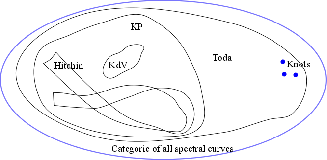
   Figure 1: The space of all spectral curves contains many classical subspaces. Some subspaces can be manifolds or orbifolds with singularities. The winding and self intersecting picture, illustrates the idea that certain subspaces, especially those with symmetry groups, can have a non–trivial topology, singular-points, self–intersections, be non–contractible, and other exotic features. We also illustrate that there is a spectral curve associated to a knot (called its $A$-polynomial), but knot spectral curves are undeformable, they are somehow ”isolated” points.   

The idea is to define our Tau function and amplitudes objectwise, independently of any subspace to which the considered spectral curve may belong, and independently of its possible deformations in a neighbourhood, and independently of any topology or structure of the space: just objectwise.

2.3 Invariants of spectral curves

Without explaining how to compute them, we recall that there is a family of ”invariants” associated to any spectral curve:

Definition 2.3 (EO invariants [32])

One associates to a spectral curve ${\cal S}$, a double sequence $\omega_{g,n}({\cal S})$ indexed by two non–negative integers $g,n$ such that $(g,n)\neq(0,0)$, of symmetric $n-$forms on ${\Sigma}^{n}$. For $n=0$, these are scalar and often denoted $\omega_{g,0}({\cal S})=\mathcal{F}_{g}({\cal S})$. We have a map defined objectwise:

$${\cal S}\mapsto\{\omega_{g,n}({\cal S})\}_{g,n}.$$ (2-12)

For $(g,n)=(0,1)$ and $(0,2)$ these are, by definition:

$$\omega_{0,1}({\cal S})={\rm y}\qquad,\qquad\omega_{0,2}({\cal S})=B.$$ (2-13)

The invariants $\omega_{g,n}({\cal S})$ with $2g-2+n>0$ are called ”stable” and the ones with $2g-2+n<0$ are called ”unstable”. The only unstable ones are $(0,1),(0,2),(1,0)$.

Let us also mention the $(0,3)$ invariant in the case $\overset{\circ}{{\Sigma}}=\mathbb{C}P^{1}$:

$$\omega_{0,3}({\cal S};z_{1},z_{2},z_{3})=\sum_{a\in\mathcal{R}}\mathop{\,\rm Res\,}_{z\to a}\frac{B(z,z_{1})B(z,z_{2})B(z,z_{3})}{d{\rm x}(z)\ d\left(\frac{{\rm y}(z)}{d{\rm x}(z)}\right)}$$ (2-14)

These invariants were defined in [32] initially only for algebraic spectral curves, and only those having only simple ramification points. But in fact the definition extends to the whole space of spectral curves, the case of higher order ramification points being defined in [14], and the algebraicity being needed nowhere in the definitions.

The case of $\mathcal{F}_{0}=\omega_{0,0}$ will be discussed below in section 3.4. We just mention that all stable invariants $\omega_{g,n}({\cal S})$ are defined by a recursion on $2g-2+n$, and involve residues at ramification points, and we refer to [32] for details, and to [50, 2] for a recent algebraic reformulation.

Theorem 2.1 (Homogeneity [32])

If $(g,n)\neq(1,0)$, the invariant $\omega_{g,n}$ is homogeneous of degree $2-2g-n$:

$$\omega_{g,n}(\lambda{\cal S})=\lambda^{2-2g-n}\omega_{g,n}({\cal S}).$$ (2-15)

And

$$\omega_{1,0}(\lambda{\cal S})=\omega_{1,0}({\cal S})+\frac{\deg\mathcal{R}}{24}\ \ln\lambda$$ (2-16)

where $\deg\mathcal{R}$ is the number (with multiplicity) of ramification points.

Theorem 2.2 (Analytic properties [32])

If $n\geq 1$ and $(g,n)\neq(0,1),(0,2)$, then $\omega_{g,n}({\cal S})$:

• is a symmetric tensor of $1$-form on ${\Sigma}^{n}$,

• has poles only at ramification points, and without residue,

$$\omega_{g,n}({\cal S})\in H^{0}({\Sigma}^{n},{\rm{Sym}}(K_{{\Sigma}}(*\mathcal{R})^{\boxtimes n}))$$ (2-17)

where $\mathcal{R}$ is the divisor of ramification points, $K_{{\Sigma}}$ is the cannonical bundle, $\boxtimes$ means a tensor product of 1-forms in each variable, and $*$ means poles of any degree.

More properties of the EO invariants –all proved in [32]– will appear along this text, and shall be introduced when needed.

2.4 Form–cycle dualities

Usually Tau-functions are defined as functions of ”times” [4], and we shall argue that times are local coordinates on $\mathcal{M}$, said otherwise, they are coordinates in the tangent space of $\mathcal{M}$, and we shall argue that they are thus coordinates in the space of meromorphic differential forms $\mathfrak{M}^{1}({\Sigma})$, and using form-cycle dualities, they are coordinates in the space of cycles, so that eventually we shall consider the Tau function as a function on the space of cycles. Let us first study the space of cycles.

2.4.1 Space of cycles

In all this section, ${\cal S}$ is kept fixed, and in particular the base curve $\overset{\circ}{{\Sigma}}$ is kept fixed, and we choose once for all an atlas of charts of $\overset{\circ}{{\Sigma}}$, each chart being an open subset of $\mathbb{C}$, so that locally in each chart there is a well defined local coordinate, in other words we do as if ${\rm x}(z)\in\mathbb{C}$ locally. Also, for each boundary $\overset{\circ}{b}$ of $\overset{\circ}{{\Sigma}}$, oriented so that the surface lies at its right, we define once for all a map $\overset{\circ}{\xi}_{\overset{\circ}{b}}:\overset{\circ}{b}\to S^{1}$ that extends analytically to a neighborhood of $\overset{\circ}{b}$.

   Figure 2: Cycles of 1st kind are usual non-contractible cycles. Cycles of 2nd kind consist of a small circle around a point, weighted by a local meromorphic function, or cycles around a boundary weighted by a local holomorphic function. Cycles of 3rd kind are chains whose boundaries are degree zero divisors. The addition of 3rd kind cycles is not commutative, an order must be choosen, encoded as an oriented graph.   

$\bullet$ 1st kind cycles:

Let $H_{1}({\Sigma},\mathbb{Z})$ (resp. $H_{1}({\Sigma},\mathbb{C})$) the integer (resp. complex) homology space of ${\Sigma}$, i.e. the space of integer (resp. complex) linear combinations of homotopy classes of closed Jordan arcs on ${\Sigma}$.

There is the usual Poincarré pairing between homology cycle $\gamma$ and 1-form $\omega$:

$$<\gamma,\omega>=\oint_{\gamma}\omega,$$ (2-18)

which shows that cycles can be viewed as elements of the dual of holomorphic 1-forms:

$$H_{1}({\Sigma},\mathbb{C})\subset\mathfrak{M}^{1}({\Sigma})^{\vee}.$$ (2-19)

These constitute ”1st kind cycles”, and we keep in mind that the space of 1st kind cycles contains an integer lattice $H_{1}({\Sigma},\mathbb{Z})\subset H_{1}({\Sigma},\mathbb{C})$.

If ${\Sigma}$ is compact and orientable, of some genus ${\mathfrak{g}}$, then $\dim H_{1}({\Sigma},\mathbb{C})=2{\mathfrak{g}}$, otherwise it is often infinite dimensional.

Remark 2.1

Notice that $H_{1}({\Sigma},\mathbb{Z})$ and $H_{1}({\Sigma},\mathbb{C})$ don’t depend on $\overset{\circ}{{\Sigma}}$, ${\rm x}$, ${\rm y}$ or $B$, they depend only on the topology of ${\Sigma}$.

We shall now enlarge the homology space of cycles, by considering a larger subset of $\mathfrak{M}^{1}({\Sigma})^{\vee}$. In section 2.4.3 below we shall provide an intrinsic definition of our space of generalized cycles, as the subset of the dual $\mathfrak{M}^{1}({\Sigma})^{\vee}$ whose pairing with $B$ is a meromorphic 1-form. But for the moment let us construct it explicitly with a basis as follows

$\bullet$ 2nd kind cycles: First we shall consider ”meromorphic currents” around marked points or boundaries, denoted: $\mathcal{C}_{p}.f$ where $\mathcal{C}_{p}$ is a ”small” counterclockwise circle around a point $p$, or around a boundary $p$ of ${\Sigma}$, and $f$ is a function holomorphic in a neighborhood of $\mathcal{C}_{p}$. If $p$ is a point, then $f$ is required to be meromorphic in a neighborhood of $p$ with a possible pole at $p$ (of any degree). $\gamma=[\mathcal{C}_{p}.f]$ is the equivalence class modulo small homotopic deformations of $\mathcal{C}_{p}$ together with analytic continuation of $f$, and we define homology classes as integer (resp. complex) linear combinations of these.

If $\omega$ is a meromorphic 1-form, and $\gamma=\mathcal{C}_{p}.f$, the following pairing is well defined, and denoted

$$<\gamma,\omega>=\oint_{\gamma}\omega=\oint_{\mathcal{C}_{p}.f}\omega=\oint_{\mathcal{C}_{p}}f\omega\qquad(=2\pi{\rm i}\,\mathop{\,\rm Res\,}_{p}f\omega\quad\text{if}\,p\,\,\text{is a point}).$$ (2-20)

These meromorphic currents are called ”2nd kind” cycles, they generate the space of second kind cycles, which is always infinite dimensional, because the degree of poles can be as high as desired.

There is also a lattice in it, indeed, if $p$ is a point, a basis of the functions $f$ meromorphic in a neighbourhood of $p$ is

$$\{\xi_{p}^{k}\}_{k\in\mathbb{Z}}\qquad,\qquad\xi_{p}=({\rm x}-{\rm x}(p))^{1/{\rm order}_{\rm x}(p)}.$$ (2-21)

The set of cycles generated by

$${\cal A}_{p,k}=\mathcal{C}_{p}.\xi_{p}^{k}\ ,\ p\in{\Sigma},\ k\geq 0$$ (2-22)

$${\cal B}_{p,k}=\frac{1}{2\pi{\rm i}\,}\mathcal{C}_{p}.\frac{\xi_{p}^{-k}}{-k}\ ,\ p\in{\Sigma},\ k\geq 1$$ (2-23)

defines a space of second kind cycles, that contains an integer lattice

$$\sum_{p\in{\Sigma}}\sum_{k\geq 0}{\cal A}_{p,k}\mathbb{Z}\oplus\sum_{p\in{\Sigma}}\sum_{k\geq 1}{\cal B}_{p,k}\mathbb{Z}.$$ (2-24)

$\bullet$ boundary 2nd kind cycles:

A boundary $b$ of ${\Sigma}$ – oriented such that the surface lies on its right – is mapped by ${\rm x}$ to a boundary $\overset{\circ}{b}$ of $\overset{\circ}{{\Sigma}}$, with winding $d_{b}\in\mathbb{Z}_{+}$, and there is a map $\xi_{\overset{\circ}{b}}:\overset{\circ}{b}\to S^{1}$ such that a neighborhood of $\overset{\circ}{b}$ is mapped to the exterior of the unit disc. We define the map $\xi_{b}:b\to S^{1}$

$$\xi_{b}(z)=\left(\xi_{\overset{\circ}{b}}({\rm x}(z))\right)^{1/d_{b}}.$$ (2-25)

The following set of cycles generate an integer lattice in the space of second kind cycles:

$${\cal A}_{b,k}=\mathcal{C}_{b}.\xi_{b}^{k}\ ,\ k\geq 0$$ (2-26)

$${\cal B}_{b,k}=\frac{1}{2\pi{\rm i}\,}\mathcal{C}_{b}\frac{\xi_{b}^{-k}}{-k}\ ,\ k\geq 1.$$ (2-27)

Remark 2.2

Notice that all integer 2nd kind cycles depend on a choice of coordinate on $\overset{\circ}{{\Sigma}}$ and on its boundaries. However, the space of complex 2nd kind cycles is independent, indeed a change of local coordinate amounts to linearly combining elements of the basis. Later, we shall consider only deformations at fixed $\overset{\circ}{{\Sigma}}$ so that the integer basis will be kept fixed.

$\bullet$ 3rd kind cycles: Then we shall also consider open chains $\gamma=\gamma_{q\to p}$ with boundary $\partial\gamma=[p]-[q]$ a divisor of degree $0$. We can define the pairing, for meromorphic 1-forms $\omega$ that have no pole at $\partial\gamma$:

$$\oint_{\gamma}\omega=<\gamma,\omega>=\int_{\gamma_{q\to p}}\omega.$$ (2-28)

For 1-forms $\omega$ that have poles at $p$ or $q$, there is a way to ”regularize” the integral of $\omega$ along $\gamma_{q\to p}$ by subtracting the poles. In order to lighten the presentation the precise definition of $\oint_{\gamma}\omega$ is provided in appendix A.

Remark 2.3

The space of 3rd kind cycles is independent of a choice of charts and coordinates in $\overset{\circ}{{\Sigma}}$.

$\bullet$ boundary 3rd kind cycles:

We also define boundary chains as follows, for a boundary $b$, we have a map $\xi_{b}:b\to S^{1}$, and we choose a point $p_{0}\in b$ such that $\xi_{p}(p_{0})=1$, and define:

$${\cal B}_{b,p_{0},0}=\frac{1}{2\pi{\rm i}\,}\gamma_{p_{0}\to p_{0}}.\ln{\xi_{b}}$$ (2-29)

with the log cut on $\mathbb{R}_{+}$. Notice that if $b$ winds $d_{p}$ times around ${\rm x}(b)$, then there exist $d_{p}$ possible choices for $p_{0}$, and if $\tilde{p}_{0}$ is another choice we have

$${\cal B}_{b,\tilde{p}_{0},0}={\cal B}_{b,p_{0},0}+\gamma_{p_{0}\to\tilde{p}_{0}},$$ (2-30)

where $\gamma_{p_{0}\to\tilde{p}_{0}}$ is the oriented boundary arc between the 2 points.

Again, one can consider linear combinations of chains, with either integer, or complex coefficients, so that there is a lattice also in the space of 3rd kind cycles.

Remark 2.4

When we consider 2 chains $\gamma_{q\to p}$ and $\gamma^{\prime}_{q^{\prime}\to p^{\prime}}$, the chain $\gamma^{\prime}_{q^{\prime}\to p^{\prime}}$ is defined in the relative homology of ${\Sigma}-\gamma_{q\to p}$, i.e. we can consider chains $\gamma^{\prime}_{q^{\prime}\to p^{\prime}}$ only relatively to the homology of $\gamma_{q\to p}$. In other words, the addition of 3rd kind cycles is not commutative, we should always tell in what order they are added.

Most of the time this non-commutativity will turn out to be irrelevant, except in multiple integrals that involve integration of forms having poles at coinciding points, in particular for double integrals of $B$ as we shall see later.

Definition 2.4 (Space of (generalized) cyles)

We define $\mathfrak{M}_{1}({\Sigma})$ as the set of linear combinations of 1st, 2nd, 3rd kind cycles. It is a $\mathbb{C}$–vector space of infinite dimension.

At fixed $\overset{\circ}{{\Sigma}}$, it contains an integer lattice $\mathfrak{M}_{1}({\Sigma},\mathbb{Z})$ as the set of integer linear combinations of integer cycles.

Remark 2.5

In section 2.4.3 below we shall see an alternative –more intrinsic– definition for the space of generalized cycles as $\mathfrak{M}_{1}({\Sigma})=\hat{B}^{-1}(\mathfrak{M}^{1}({\Sigma}))$, i.e. the space of elements of the dual $\mathfrak{M}^{1}({\Sigma})^{\vee}$ whose pairing with $B$ is a meromorphic 1-form.

2.4.2 Intersection and symplectic structure

On 1st kind cycles is defined the intersection $\gamma\cap\gamma^{\prime}=-\gamma^{\prime}\cap\gamma$, as the algebraic counting of oriented crossings of transverse Jordan arcs representative of the cycles.

We shall extend it to 2nd kind and 3rd kind cycles in the following way

Definition 2.5 (Intersection)

We define the intersection form as an antisymmetric bilinear form on $\mathfrak{M}_{1}({\Sigma})\times\mathfrak{M}_{1}({\Sigma})\to\mathbb{C}$ (resp. $\mathfrak{M}_{1}({\Sigma},\mathbb{Z})\times\mathfrak{M}_{1}({\Sigma},\mathbb{Z})\to\mathbb{Z}$), as follows.

We define the intersection of 1st kind cycles as the usual crossing number, and also the intersection of 1st kind and 3rd kind as the usual crossing number of a cycle with a chain in the relative homology. For the intersection of two 3rd kind paths with distinct boundaries we define the intersection as the crossing number, and if the boundaries are not distinct the crossing number multiplied by $\frac{1}{2}$, for example if both paths end at $p$

$$\gamma_{q\to p}\cap\gamma^{\prime}_{q^{\prime}\to p}=\pm\ \frac{1}{2}$$ (2-31)

where $\pm 1$ is, like in usual crossing numbers, the respective orientation of the second Jordan arc with respect to the first one.

Then we define the other intersections by the following table (completed by antisymmetry):

kind	1st	3rd	2nd
	$\gamma^{\prime}$	$\gamma^{\prime}_{q^{\prime}\to p^{\prime}}$	$\mathcal{C}^{\prime}_{p^{\prime}}.f^{\prime}$
$\gamma$	$\gamma\cap\gamma^{\prime}$	$\gamma\cap\gamma^{\prime}_{q^{\prime}\to p^{\prime}}$	$\gamma\cap\mathcal{C}_{p^{\prime}}.f^{\prime}=0$
$\gamma_{q\to p}$		$\begin{array}[]{l}\gamma_{q\to p}\cap\gamma^{\prime}_{q^{\prime}\to p^{\prime}}\cr\pm\frac{\delta_{p,p^{\prime}}}{2}\pm\frac{\delta_{q,q^{\prime}}}{2}\cr\pm\frac{\delta_{p,q^{\prime}}}{2}\pm\frac{\delta_{q,p^{\prime}}}{2}\end{array}$	$\gamma_{q\to p}\cap\mathcal{C}_{p^{\prime}}.f^{\prime}=\left\{\begin{array}[]{l}0\,\,\,\,{\rm if}\,\,f^{\prime}(p^{\prime})=\infty\cr(\delta_{q,p^{\prime}}-\delta_{p,p^{\prime}})f^{\prime}(p^{\prime})\end{array}\right.$
$\mathcal{C}_{p}.f$			$\delta_{p,p^{\prime}}\oint_{\mathcal{C}_{p}}f\ df^{\prime}$

Notice that it indeed takes integer values on $\mathfrak{M}_{1}({\Sigma},\mathbb{Z})\times\mathfrak{M}_{1}({\Sigma},\mathbb{Z})$. In particular, with the basis (2-22)

$${\cal A}_{p,k}\cap{\cal B}_{p^{\prime},k^{\prime}}=\delta_{p,p^{\prime}}\delta_{k,k^{\prime}}.$$ (2-32)

Except 3rd kind cycles that can have half–integer intersections. This is illustrated in fig. 3

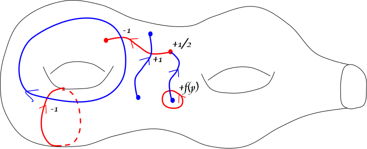
   Figure 3: Intersections of cycles blue $\cap$ red.   

There is an alternative way to define or compute intersections:

Proposition 2.1

We have

$$\oint_{\gamma}\oint_{\gamma^{\prime}}B-\oint_{\gamma^{\prime}}\oint_{\gamma}B=2\pi{\rm i}\,\ \gamma\cap\gamma^{\prime}.$$ (2-33)

As a consequence:

$$\mathcal{Q}(\gamma,\gamma^{\prime})=\frac{1}{2\pi{\rm i}\,}\oint_{\gamma}\oint_{\gamma^{\prime}}B-\frac{1}{2}\ \gamma\cap\gamma^{\prime}$$ (2-34)

is a symmetric bilinear form on $\mathfrak{M}_{1}({\Sigma})\times\mathfrak{M}_{1}({\Sigma})$.

proof:    It is easy to verify that it holds for every pair of cycles in the basis used to define $\mathfrak{M}_{1}({\Sigma})$.

Let us recall the proof for elements of $H_{1}({\Sigma},\mathbb{Z})$. Choose some transversally crossing Jordan arcs representatives. Away from intersection points the order of integrations can be exchanged. In a neighborhood of intersection points, we have the behaviour (2-5), $B(z,z^{\prime})\sim\frac{\kappa}{2}dzdz^{\prime}/(z-z^{\prime})^{2}+\text{analytic}=\frac{\kappa}{2}d_{z}d_{z^{\prime}}\log(z-z^{\prime})+\text{analytic}$ in any local coordinates. The difference of orders of integration yields the discontinuity of the log, namely $\pm\kappa\pi{\rm i}\,$ depending on the orientation. If we choose the behaviour (2-6), we get $2\pi{\rm i}\,\gamma\cap\gamma^{\prime}$. If instead of (2-6), we would choose $\kappa\neq 2\ \text{Id}$, this would define a generalized intersection theory for Cameral covers, that is considered in details in .

2.4.3 Forms $\longleftrightarrow$ cycles

The bilinear differential $B$ allows to define a ”form–cycle duality”:

Definition 2.6 (Map $\hat{B}$: cycles $\longrightarrow$ 1-forms)

The integral –in the 1st projection– of the 2nd kind differential $B$ along a cycle is a meromorphic 1-form of the 2nd projection, of the same kind as the cycle: 1st kind $\to$ no poles, 3rd kind $\to$ simple poles, 2nd kind $\to$ poles of degree $\geq 2$. This defines a linear map from the space of cycles to meromorphic 1-forms on ${\Sigma}$

$$\hat{B}:\mathfrak{M}_{1}({\Sigma}) {\to} \mathfrak{M}^{1}({\Sigma})$$ (2-35)

$$\gamma \mapsto \oint_{\gamma}B.$$ (2-36)

We shall prove below that the map $\hat{B}$ is surjective, which shows that $\mathfrak{M}_{1}({\Sigma})=\hat{B}^{-1}(\mathfrak{M}^{1}({\Sigma}))$ as mentioned in remark 2.5. It is not injective, we shall see that it has a huge kernel.

Now we shall define a map $\hat{C}$: 1-forms $\to$ cycles, playing the role of a right inverse of $\hat{B}$. If we would have a finite basis of cycles $\Gamma_{i}$, with intersection matrix $I_{i,j}=\Gamma_{i}\cap\Gamma_{j}$ we would define the map $\hat{C}$ as

$$\hat{C}(\omega)=\frac{1}{2\pi{\rm i}\,}\sum_{i,j}\Gamma_{i}\ (I^{-1})_{i,j}\ \left(\oint_{\Gamma_{j}}\omega\right)\$$ (2-37)

which is invariant under changes of basis. Unfortunately, expression 2-37 is meaningless because the space $\mathfrak{M}_{1}({\Sigma})$ is infinite dimensional. But given a meromorphic $\omega$, it is possible (this is what the definition of $\hat{C}$ below does) to find a basis well adapted to $\omega$, such that only finitely many terms are not vanishing in the sum, or sums are absolutely convergent (in particular Fourier series at the boundaries), so in practice formula 2-37 can be applied. In a symplectic basis $I_{i,j}={\cal A}_{i}\cap{\cal B}_{j}=\delta_{i,j}$ we would have

$$\hat{C}(\omega)=\sum_{i}t_{i}(\omega){\cal B}_{i}\qquad\text{with}\qquad t_{i}(\omega)=\frac{1}{2\pi{\rm i}\,}\oint_{{\cal A}_{i}}\omega,$$ (2-38)

it is such that

$$\omega=\hat{B}(\hat{C}(\omega))=\sum_{i}t_{i}(\omega)\hat{B}({\cal B}_{i}).$$ (2-39)

Now we give the actual intrinsic definition of the map $\hat{C}$:

Definition 2.7 (Map $\hat{C}$: 1-forms $\longrightarrow$ cycles)

If ${\Sigma}=\cup_{i}{\Sigma}_{i}$ is a union of connected components, choose a generic point $o_{i}\in{\Sigma}_{i}$, and a fundamental domain of ${\Sigma}_{i}-\{o_{i}\}$ i.e. ${\Sigma}_{i}-\Gamma_{i}$ a 1-face cellular graph $\Gamma_{i}$ (for which $o_{i}$ is a 1-valent vertex). The graph $\Gamma=\cup_{i}\Gamma_{i}$ has 2 kinds of edges: internal edges, and boundary edges that lie on $\partial{\Sigma}$. On each internal edge $e$, choose a point $p_{e}$, corresponding to 2 points $p_{e\pm}$ in the fundamental domain, with $p_{e+}$ on the left of $e$ and $p_{e-}$ on the right. Let $e^{\perp}=\gamma_{p_{e-}\to p_{e+}}$ the unique (up to homotopy) arc from $p_{e-}$ to $p_{e+}$ in the fundamental domain. We also identify $e^{\perp}$ with the homology class of a 1st kind cycle on ${\Sigma}$.

Then for a given choice of fundamental domain, define, for every meromorphic 1-form $\omega\in\mathfrak{M}^{1}({\Sigma})$:

• For every pole $p$ of $\omega$, of degree $d_{p}\geq 1$, and every $j\geq 0$:

  $$t_{p,j}=\mathop{\,\rm Res\,}_{p}(\xi_{p})^{j}\ \omega=\frac{1}{2\pi{\rm i}\,}\oint_{{\cal A}_{p,j}}\omega$$ (2-40)

  the $t_{p,j}$s are called the ”KP times” (see def.2.9).

  We assumed the number of poles $p$ finite. Also all times with $j\geq\deg_{p}\omega$ are vanishing, only a finite number of times are non-zero.

• define

  $$\tilde{\omega}=\omega-\sum_{i}\sum_{p=\text{poles of}\ \omega\text{ in }{\Sigma}_{i}}\left(t_{p,0}\hat{B}(\gamma_{o_{i}\to p})+\sum_{j=1}^{\deg_{p}\omega-1}t_{p,j}\hat{B}({\cal B}_{p,j})\right)$$ (2-41)

  $\tilde{\omega}$ is holomorphic on ${\Sigma}$, it has no poles.

• In the fundamental domain of ${\Sigma}_{i}-\{o_{i}\}$, choose some generic points $o^{\prime}_{i}$, and define the holomorphic function

  $$\tilde{f}(z)=\int_{o^{\prime}_{i}}^{z}\tilde{\omega}.$$ (2-42)

• Then define

  $$\begin{array}[]{llll}\hat{C}(\omega)&\overset{\text{def}}{=}&\sum_{i}\sum_{p=\text{poles of}\ \omega\text{ in }{\Sigma}_{i}}t_{p,0}\gamma_{o_{i}\to p}&\quad\to\quad\text{3rd kind}\cr&&-\sum_{p=\text{poles of}\ \omega}\sum_{j=1}^{\deg_{p}\omega-1}\frac{t_{p,j}}{2\pi{\rm i}\,}\ \mathcal{C}_{p}.\frac{\xi_{p}^{-j}}{j}&\quad\to\quad\text{2nd kind}\cr&&+\frac{1}{2\pi{\rm i}\,}\sum_{e=\text{internal edges}}(\oint_{e^{\perp}}\tilde{\omega})e&\quad\to\quad\text{3rd + 1st kind}\cr&&+\frac{1}{2\pi{\rm i}\,}\sum_{e=\text{boundary edges}}e.\tilde{f}&\quad\to\quad\text{2nd kind}.\end{array}$$ (2-43)

  Notice that the 3rd line may yield 1st kind cycles because a sum of open chains can be a closed cycle.

  In the neighborhood of a boundary $b$ with its map $\xi_{b}:b\to S^{1}$, choose $p_{0}$ a boundary edge endpoint on $b$, then $\tilde{f}(z)-\frac{1}{2\pi{\rm i}\,}\left(\oint_{b}\omega\right)\log(\xi_{b}(z)/\xi_{b}(p_{0}))$ – with the log’s cut on $\mathbb{R}_{+}$ – is a periodic function on $b$, that can be decomposed into its Fourier modes:

  $$\tilde{f}(z)=\frac{1}{2\pi{\rm i}\,}\left(\oint_{b}\omega\right)\log(\xi_{b}(z)/\xi_{b}(p_{0}))+\sum_{k\in\mathbb{Z}}t_{b,k}\xi_{b}(z)^{k}.$$ (2-44)

  This shows that $\hat{C}(\omega)$ is a linear combination of all types of cycles introduced in section 2.4.1, therefore

  $$\hat{C}(\omega)\in\mathfrak{M}_{1}({\Sigma}).$$ (2-45)

Lemma 2.1

The map:

$$\hat{C}:\mathfrak{M}^{1}({\Sigma}) \to \mathfrak{M}_{1}({\Sigma})$$ (2-46)

$$\omega \mapsto \hat{C}(\omega)$$ (2-47)

is linear and is independent of a choice of fundamental domain and of the choice of $o^{\prime}_{i}$.

Moreover it satisfies for every $\omega$:

$$\omega=\hat{B}(\hat{C}(\omega)).$$ (2-48)

proof:    In appendix B. The fact that $\omega=\hat{B}(\hat{C}(\omega))$ is in fact the Riemann bilinear identity. $\square$

Corollary 2.1

$$\Pi=\hat{C}\circ\hat{B}\qquad\text{is a projector}\qquad\Pi^{2}=\Pi.$$ (2-49)

$\hat{C}$ is injective. $\hat{B}$ is surjective. We have the exact sequence

$$0\to{\rm Ker\ }\hat{B}\to\mathfrak{M}_{1}({\Sigma}) \overset{\hat{B}}{\to} \mathfrak{M}^{1}({\Sigma})\to 0$$ (2-50)

We have an isomorphism $\mathfrak{M}^{1}({\Sigma})\sim\mathfrak{M}_{1}({\Sigma})/{\rm Ker\ }\hat{B}$.

The map $\Pi=\hat{C}\circ\hat{B}:\mathfrak{M}_{1}({\Sigma})\to\mathfrak{M}_{1}({\Sigma})$ is a projector on ${\rm Im\ }\Pi\sim\mathfrak{M}_{1}({\Sigma})/{\rm Ker\ }\hat{B}$, parallel to ${\rm Ker\ }\hat{B}$. The map $\text{Id}-\Pi$ is the projector on ${\rm Ker\ }\hat{B}$ parallel to ${\rm Im\ }\Pi$.

We have

$$\mathfrak{M}_{1}({\Sigma})={\rm Im\ }\Pi\oplus{\rm Ker\ }\hat{B}.$$ (2-51)

Proposition 2.2

Both ${\rm Ker\ }\hat{B}$ and $\operatorname{Im}\Pi$ are Lagrangian submanifolds of $\mathfrak{M}_{1}({\Sigma})$.

$\mathfrak{M}_{1}({\Sigma})=\operatorname{Im}\Pi\oplus{\rm Ker\ }\hat{B}$ is a Lagrangian decomposition.

proof:    In appendix C. Notice that ${\rm Ker\ }\hat{B}$ Lagrangian is a trivial consequence of prop.2.1. $\square$

Notice that all 2nd kind cycles ${\cal A}_{p,k}$ with $k\geq 0$ are in ${\rm Ker\ }\hat{B}$, whereas the 2nd kind cycles ${\cal B}_{p,k}$ involving negative powers of $\xi_{p}^{-k}$ are not in ${\rm Ker\ }\hat{B}$.

Proposition 2.3 (proved in [32])

If $\gamma\in{\rm Ker\ }\hat{B}$, we have for all $n\geq 1$ and $(g,n)\neq(0,1)$:

$$\int_{z_{1}\in\gamma}\omega_{g,n}(z_{1},z_{2},\dots,z_{n})=0.$$ (2-52)

This holds by definition for $\omega_{0,2}=B$.

The map $\gamma\mapsto\int_{\gamma}\omega_{0,1}$ has a kernel, which usually differs from ${\rm Ker\ }\hat{B}$.

2.4.4 Positivity

We define a complex structure on the space of cycles by complexifying integer cycles:

$$\mathfrak{M}_{1}({\Sigma},\mathbb{C})=\mathfrak{M}_{1}({\Sigma},\mathbb{Z})\otimes\mathbb{C},$$ (2-53)

we define the complex conjugate by acting only on the $\mathbb{C}$ factor. In other words, if $\gamma=\sum_{i}t_{i}\gamma_{i}$, with $\gamma_{i}$ independent integer cycles and $t_{i}\in\mathbb{C}$, we define its complex conjugate as

$$\bar{\gamma}=\sum_{i}\bar{t_{i}}\gamma_{i}.$$ (2-54)

This is independent of a choice of integer decomposition.

Then:

Lemma 2.2

The quadratic form $-2\pi{\rm i}\,\mathcal{Q}$ defined in prop.2.1 is a positive definite Hermitian form on ${\rm Im\ }\Pi$, for $\Pi(\gamma)\neq 0$:

$$-2\pi{\rm i}\,\ \mathcal{Q}(\Pi(\gamma),\overline{\Pi(\gamma)})>0.$$ (2-55)

proof:    In appendix D. This is a generalization of the Riemann bilinear inequality proving that $\Im\tau>0$, it is proved likewise using Riemann bilinear identity and Stokes theorem. $\square$

2.5 Lagrangian submanifolds and Darboux coordinates

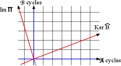
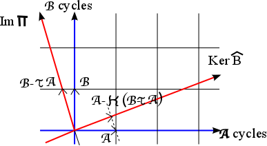
        Figure 4: Consider ${\cal A}$-cycles and ${\cal B}$-cycles forming a symplectic basis of the lattice of integer cycles. ${\rm Ker\ }\hat{B}$ and ${\rm Im\ }\Pi$ are orthogonal Lagrangian submanifolds, and ${\rm Im\ }\Pi$ is never parallel to the lattice. A convenient basis for ${\rm Im\ }\Pi$ is to project ${\cal B}$-cycles parallel to ${\cal A}$, and a basis for ${\rm Ker\ }\hat{B}$ is to project ${\cal A}$-cycles parallel to ${\rm Im\ }\Pi$.   

Definition 2.8 (Darboux basis)

A Darboux decomposition is $\mathfrak{M}_{1}({\Sigma})={\cal A}({\Sigma})\oplus{\cal B}({\Sigma})$, with ${\cal A}({\Sigma})$ and ${\cal B}({\Sigma})$ both Lagrangian. An integer Darboux decomposition is $\mathfrak{M}_{1}({\Sigma},\mathbb{Z})={\cal A}({\Sigma},\mathbb{Z})\oplus{\cal B}({\Sigma},\mathbb{Z})$ with ${\cal A}({\Sigma},\mathbb{Z})$ and ${\cal B}({\Sigma},\mathbb{Z})$ both integer Lagrangian sublattices. Then it is possible (not unique) to choose a Darboux Basis of cycles such that

$${\cal A}_{i}\in{\cal A}({\Sigma})\quad,\quad{\cal B}_{i}\in{\cal B}({\Sigma})$$ (2-56)

$${\cal A}_{i}\cap{\cal A}_{j}=0\quad,\quad{\cal B}_{i}\cap{\cal B}_{j}=0\quad,\quad{\cal A}_{i}\cap{\cal B}_{j}=\delta_{i,j}$$ (2-57)

i.e. the intersection matrix takes the block–form

$$\begin{pmatrix}0&{\rm Id}\cr-{\rm Id}&0\end{pmatrix}.$$

We have several usual decompositions:

1. The decomposition $\mathfrak{M}_{1}({\Sigma})={\rm Im\ }\Pi\oplus{\rm Ker\ }\hat{B}$ is canonical, it is Darboux but not integer. There is no canonical Darboux basis in it. Moreover, ${\rm Ker\ }\hat{B}$ and ${\rm Im\ }\Pi$ both get deformed under deformations of the spectral curve. This Darboux decomposition, although canonical, is not very convenient for defining a connection on the bundle of cycles $\mathfrak{M}_{1}\to\mathcal{M}$.

2. Due to lemma 2.2, $\Im{\rm Im\ }\Pi$ and $\Re{\rm Im\ }\Pi$ are transverse and provide another canonical decomposition:

   $$\mathfrak{M}_{1}({\Sigma})=\Im{\rm Im\ }\Pi\oplus\Re{\rm Im\ }\Pi.$$

   This decomposition is real but is not integer, and there is no canonical Darboux basis in it, and it also gets deformed under deformations of the spectral curve.

3. There exists integer Darboux basis $\mathfrak{M}_{1}({\Sigma},\mathbb{Z})={\cal A}({\Sigma},\mathbb{Z})\oplus{\cal B}({\Sigma},\mathbb{Z})$ (we have constructed one in section 2.4.1). Any such decomposition is rigid but is not canonical. Going from one choice to another is called a modular transformation.

   Due to lemma 2.2, ${\rm Im\ }\Pi$ is always transverse to that decomposition. A basis of ${\rm Im\ }\Pi$ can be obtained by projecting ${\cal B}({\Sigma},\mathbb{Z})$ parallel to ${\cal A}({\Sigma},\mathbb{Z})$, i.e. for each ${\cal B}_{i}$, find a linear combination $\sum_{j}\tau_{i,j}{\cal A}_{j}$ such that

   $${\cal B}^{\prime}_{i}={\cal B}_{i}-\sum_{j}\tau_{i,j}{\cal A}_{j}\in{\rm Im\ }\Pi.$$ (2-58)

   Lemma 2.2 implies that the matrix $\tau_{i,j}$ is symmetric and $\Im\tau>0$. In particular $\tau\neq 0$. We can get a basis of ${\rm Ker\ }\hat{B}$ by projecting ${\cal A}({\Sigma},\mathbb{Z})$ parallel to ${\rm Im\ }\Pi$. Define

   $$\kappa_{i,j}={\cal A}_{i}\cap\Pi({\cal A}_{j}),$$ (2-59)

   then

   $${\cal A}^{\prime}_{i}={\cal A}_{i}-\sum_{j}\kappa_{i,j}{\cal B}^{\prime}_{j}\in{\rm Ker\ }\hat{B}.$$ (2-60)

   The basis

   $$({\cal A}^{\prime}_{i},{\cal B}^{\prime}_{i})$$ (2-61)

   is Darboux, but not integer ($\tau$ can never be integer since $\Im\tau>0$), and it gets deformed under deformations of the spectral curve. In this basis we have

   $$\mathcal{Q}({\cal A}^{\prime}_{i},{\cal A}^{\prime}_{j})=0\qquad,\qquad\mathcal{Q}({\cal A}^{\prime}_{i},{\cal B}^{\prime}_{j})=\frac{1}{2}\ \delta_{i,j}\qquad,\qquad\mathcal{Q}({\cal B}^{\prime}_{i},{\cal B}^{\prime}_{j})=0.$$ (2-62)

   Remark 2.6

   The matrices $\tau$ and $\kappa$ are infinite dimensional. However, it is possible to choose ${\cal A}({\Sigma},\mathbb{Z})$ that differs from ${\rm Ker\ }\hat{B}$ by at most a finite dimension space. For example, it suffices to choose ${\cal A}({\Sigma},\mathbb{Z})$ (resp. ${\cal B}({\Sigma},\mathbb{Z})$) containing all but a finite number of positive (resp. negative) 2nd kind cycles, and completed with a finite number of negative (resp. positive) cycles. In this case the matrices $\tau$ and $\kappa$ have only a finite dimensional non-trivial part.

4. Define ${\cal A}^{\prime\prime}_{i}$ the projection of ${\cal A}_{i}$ onto ${\rm Ker\ }\hat{B}$, parallel to ${\cal B}({\Sigma},\mathbb{Z})$

   $${\cal A}^{\prime\prime}_{i}={\cal A}_{i}-\sum_{j}X_{i,j}{\cal B}_{j}\in{\rm Ker\ }\hat{B}.$$ (2-63)

   The symmetric matrix $X_{i,j}$ is related to the matrices $\tau$ and $\kappa$ above by

   $$X=(1+\kappa\tau)^{-1}\kappa.$$ (2-64)

   Then, the basis

   $$({\cal A}^{\prime\prime}_{i},{\cal B}_{i})$$ (2-65)

   is Darboux, but not necessarily integer. However, we shall see below that it is rigid under ”Rauch” deformations of the spectral curve. We define the projection on ${\cal B}({\Sigma},\mathbb{Z})$ parallel to ${\rm Ker\ }\hat{B}$:

   $$\Pi_{{\cal B}({\Sigma},\mathbb{Z})}({\cal B}_{i})={\cal B}_{i}\qquad,\qquad\Pi_{{\cal B}({\Sigma},\mathbb{Z})}({\cal A}^{\prime\prime}_{i})=0.$$ (2-66)

   In this basis we have

   $$\mathcal{Q}({\cal A}^{\prime\prime}_{i},{\cal A}^{\prime\prime}_{j})=0\qquad,\qquad\mathcal{Q}({\cal A}^{\prime\prime}_{i},{\cal B}_{j})=\frac{1}{2}\ \delta_{i,j}\qquad,\qquad\mathcal{Q}({\cal B}_{i},{\cal B}_{j})=R_{i,j}$$ (2-67)

   with the matrix $R$ defined below.

5. Define the symmetric matrix

   $$R=\tau(1-X\tau)^{-1},$$ (2-68)

   and

   $${\cal B}^{\prime\prime}_{i}={\cal B}_{i}-\sum_{j}R_{i,j}{\cal A}^{\prime\prime}_{j}=(1-\tau X)^{-1}{\cal B}^{\prime}_{i}\in{\rm Im\ }\hat{C}.$$ (2-69)

   The basis

   $$({\cal A}^{\prime\prime}_{i},{\cal B}^{\prime\prime}_{i})$$ (2-70)

   is Darboux, but not integer. It is a Lagrangian decomposition of ${\rm Ker\ }\hat{B}\oplus{\rm Im\ }\Pi$. It is not rigid under Rauch deformations, because $\tau_{i,j}$ is not.

   In this basis we have

   $$\mathcal{Q}({\cal A}^{\prime\prime}_{i},{\cal A}^{\prime\prime}_{j})=0\qquad,\qquad\mathcal{Q}({\cal A}^{\prime\prime}_{i},{\cal B}^{\prime\prime}_{j})=\frac{1}{2}\ \delta_{i,j}\qquad,\qquad\mathcal{Q}({\cal B}^{\prime\prime}_{i},{\cal B}^{\prime\prime}_{j})=0.$$ (2-71)

In each decomposition, choosing a basis, allows to introduce time coordinates parametrizing cycles and forms

Remark 2.7

Observe that, since several of the decompositions introduced here depend on integers or on reals, then going from one decomposition to another, changes the coordinates (the times) in a possibly not analytic way. This is related to the existence of several complex structures in our moduli space. This is the origin of the HyperKähler structure of the moduli space.

2.5.1 Times and periods of Darboux coordinates

Having choosen a Darboux basis of cycles $({\cal A},{\cal B})$,

Definition 2.9

we define the times as the periods of ${\rm y}$ over ${\cal A}$–cycles:

$$t_{i}=\frac{1}{2\pi{\rm i}\,}\oint_{{\cal A}_{i}}{\rm y}.$$ (2-72)

In many known examples, these times are indeed the ”good” times of our system. For example, if ${\rm y}$ is meromorphic with a pole at $p$, and with Laurent series expansion near $p$ as

$${\rm y}(z)\mathop{\sim}_{z\to p}\sum_{k=0}^{\deg_{p}{\rm y}}t_{p,k}\xi_{p}(z)^{-k-1}d\xi_{p}(z)+\text{analytic at }p,$$ (2-73)

the coefficients $t_{p,k}$ are the ${\cal A}_{p,k}$ periods

$$t_{p,k}=\frac{1}{2\pi{\rm i}\,}\oint_{{\cal A}_{p,k}}{\rm y}.$$ (2-74)

These are called the KP times.

2.5.2 Example with compact surfaces

Consider a case where ${\Sigma}$ is compact of genus ${\mathfrak{g}}$, with a symplectic basis of 1st kind cycles $({\cal A}_{i},{\cal B}_{i})_{i=1,\dots,{\mathfrak{g}}}$, and define ${\cal A}^{\prime\prime}_{i}$ as in (2-65). Define $\omega_{i}$ the holomorphic basis of 1-forms such that $\oint_{{\cal A}_{i}}\omega_{j}=\delta_{i,j}$ and define the period matrix $\tau_{i,j}=\oint_{{\cal B}_{i}}\omega_{j}=\tau_{j,i}$, it actually coincides with the one in (2-58). Consider also the case where

$$B(z,z^{\prime})=d_{z}d_{z^{\prime}}\log\theta_{c}(\mathfrak{a}(z)-\mathfrak{a}(z^{\prime});\tau)+2\pi{\rm i}\,\sum_{i,j=1}^{{\mathfrak{g}}}\kappa_{i,j}\omega_{i}(z)\omega_{j}(z^{\prime})$$ (2-75)

with $\mathfrak{a}=(\mathfrak{a}_{1},\dots,\mathfrak{a}_{\mathfrak{g}})$ the Abel map (defined by $d\mathfrak{a}_{i}=\omega_{i}$) and $c$ a regular odd characteristic, and $\theta$ the Siegel Theta function. The symmetric ${\mathfrak{g}}\times{\mathfrak{g}}$ matrix $\kappa_{i,j}$ coincides with the one introduced in (2-60).

We have:

$$\hat{B}({\cal A}^{\prime}_{i})=\hat{B}({\cal A}^{\prime\prime}_{i})=0$$ (2-76)

$$\hat{B}({\cal B}^{\prime}_{i})=2\pi{\rm i}\,\omega_{i}\qquad,\quad\hat{B}({\cal B}_{i})=\hat{B}({\cal B}^{\prime\prime}_{i})=2\pi{\rm i}\,\sum_{j}(1+\tau\kappa)_{i,j}\omega_{j}.$$ (2-77)

Writing the Taylor expansion of $B$ near a point $p\in{\Sigma}$ as

$$B(z,z^{\prime})-\frac{d\xi_{p}(z)d\xi_{p}(z^{\prime})}{(\xi_{p}(z)-\xi_{p}(z^{\prime}))^{2}}\sim\sum_{k,l=1}^{\infty}kl\ \tau_{p,k;p,l}\xi_{p}(z)^{k-1}\xi_{p}(z^{\prime})^{l-1}\,d\xi_{p}(z)d\xi_{p}(z^{\prime})$$ (2-78)

we get

$$\hat{B}({\cal A}_{p,k})=0\qquad,\qquad\hat{B}({\cal B}_{p,k})=\left(\xi_{p}^{-k-1}+\sum_{l=1}^{\infty}l\tau_{p,k;p,l}\ \xi_{p}^{l-1}\right)d\xi_{p}\quad\text{near }p.$$ (2-79)

$$\hat{B}(\gamma_{q\to p})=\int_{q}^{p}B=\left(\xi_{p}^{-1}+\sum_{l=1}^{\infty}l\tau_{p,0;p,l}\ \xi_{p}^{l-1}\right)d\xi_{p}\quad\text{near }p.$$ (2-80)

In both cases near another point $p^{\prime}\neq p$, these forms are analytic and have a regular Taylor expansion that we write

$$\hat{B}({\cal B}_{p,k})=\sum_{l=1}^{\infty}l\tau_{p,k;p^{\prime},l}\ \xi_{p^{\prime}}^{l-1}d\xi_{p^{\prime}}\quad\text{near }p^{\prime},$$ (2-81)

where the matrix $\tau$ coincides with that of (2-58).

In the Darboux basis (2-65) we have:

$$\mathcal{Q}({\cal A}^{\prime\prime}_{i},{\cal A}^{\prime\prime}_{j})=0\quad,\quad\mathcal{Q}({\cal A}^{\prime\prime}_{i},{\cal B}_{j})=\frac{1}{2}\ \delta_{i,j}\quad,\quad\mathcal{Q}({\cal B}_{i},{\cal B}_{j})=R_{i,j}$$ (2-82)

For 3rd kind cycles, introducing the prime form (see [36]) we have:

$$2\pi{\rm i}\,\mathcal{Q}(\gamma_{q\to p},\gamma^{\prime}_{q^{\prime}\to p^{\prime}})=\ln{\frac{E(p,p^{\prime})E(q,q^{\prime})}{E(q,p^{\prime})E(p,q^{\prime})}}$$ (2-83)

$$2\pi{\rm i}\,\mathcal{Q}(\gamma_{q\to p},\gamma^{\prime}_{q^{\prime}\to p})=\ln{\frac{E(q,q^{\prime})}{E(q,p)E(p,q^{\prime})d\xi_{p}(p)}}$$ (2-84)

$$2\pi{\rm i}\,\mathcal{Q}(\gamma_{q\to p},\gamma_{q\to p})=\ln{\frac{-1}{E(q,p)^{2}d\xi_{p}(p)d\xi_{q}(q)}}$$ (2-85)

$$2\pi{\rm i}\,\mathcal{Q}(\sum_{i=1}^{k}\alpha_{i}\gamma_{q_{i}\to p_{i}},\sum_{i=1}^{k}\alpha_{i}\gamma_{q_{i}\to p_{i}})=\ln{\frac{\prod_{i<j}E(p_{i},p_{j})^{\alpha_{i}\alpha_{j}}\prod_{i<j}E(q_{i},q_{j})^{\alpha_{i}\alpha_{j}}}{\prod_{i,j}E(p_{i},q_{j})^{\alpha_{i}\alpha_{j}}\prod_{i}d\xi_{p_{i}}(p_{i})^{\alpha_{i}^{2}}d\xi_{q_{i}}(q_{i})^{\alpha_{i}^{2}}}}$$ (2-86)

We see here that indeed the result depends on an ordering $i<j$, echoing remark 2.4. A different choice of ordering changes the result by $\pi{\rm i}\,$ times an integer quadratic polynomials of the $\alpha_{i}$s. In particular if the $\alpha_{i}$s are integer, a change of ordering just changes the result modulo $\pi{\rm i}\,\mathbb{Z}$, i.e. a sign inside the log.

3 Deformations of spectral curves

We shall consider deformations of spectral curves at fixed ${\Sigma}$ (as a topological surface) and fixed base $\overset{\circ}{{\Sigma}}$. We can therefore deform ${\rm x}$, ${\rm y}$ or $B$. The deformation of ${\rm x}$ induces a deformation of the complex structure of ${\Sigma}$ as a Riemann surface whose complex structure is the pullback by ${\rm x}$ of $\overset{\circ}{{\Sigma}}$.

The idea developed below, is that deformations –here we mean tangent vectors– of ${\rm y}$ are 1-forms (resp. deformations of $B$ are $1\boxtimes 1$–forms) and are dual to cycles (resp. dual to tensor products of cycles). This will allow to identify the tangent space $T_{{\cal S}}{\mathcal{M}}$ with a subspace of cycles $\mathfrak{M}_{1}({\Sigma},\mathbb{Z})\otimes\mathbb{C}$ (resp. pairs of cycles). Moreover, since at fixed base $\overset{\circ}{{\Sigma}}$, integer cycles form a lattice, they are rigid and don’t deform, this will induce a trivial connexion on the cycles bundle.

3.1 Meromorphic tangent space

The space $\mathcal{M}$ of all spectral curves is too large and is not a manifold, in particular it doesn’t always have a tangent space at a point. However, given a spectral curve, we shall consider a subspace, that is locally a manifold and has a tangent space. In this purpose we shall restrict to only a subset of possible deformations, those locally meromorphic.

Definition 3.1 (Subspace of Meromorphic shifts of a spectral curve.)

Given a spectral curve ${\cal S}$ represented by the data $({\Sigma},{\rm x},{\rm y},B)$, consider the subspace ${\mathcal{M}}_{{{\cal S}}+\text{mero}}$ whose objects are spectral curves $\tilde{\cal S}=[({\Sigma},\tilde{\rm x},\tilde{\rm y},\tilde{B})]$ with the same topological surface ${\Sigma}$, with the same base Riemann surface $\overset{\circ}{{\Sigma}}$ for ${\rm x}$ and $\tilde{\rm x}$, and such that $\tilde{\rm x}-{\rm x}$, $\tilde{\rm y}-{\rm y}$, $\tilde{B}-B$ are $C^{\infty}$ plus at most a finite number of singularities, and such that at points where ${\rm x}$ and $\tilde{\rm x}$ are locally invertible, ${\rm y}\circ{\rm x}^{-1}-\tilde{\rm y}\circ\tilde{\rm x}^{-1}$ is locally meromorphic on $\overset{\circ}{{\Sigma}}$, and similarly ${\rm x}_{*}B-\tilde{\rm x}_{*}\tilde{B}$ is locally a bi-holomorphic differential on $\overset{\circ}{{\Sigma}}\times\overset{\circ}{{\Sigma}}$ (these are in general not holomorphic at branchpoints of ${\rm x}$ or $\tilde{\rm x}$).

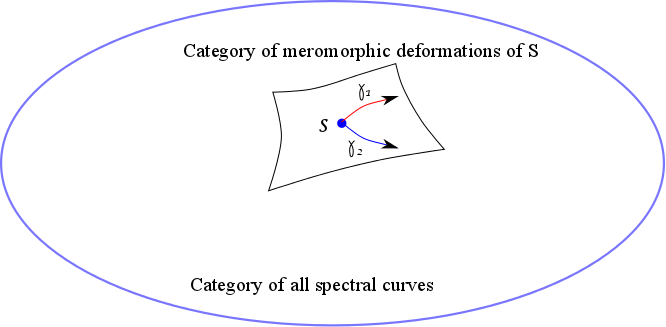
   Figure 5: The subspace of meromorphic deformations of a spectral curve. Tangent vectors are cycles, and thus cycles generate flows.   

This subspace is a quotient (mod diffeomorphisms) of an affine bundle ${\cal S}+\mathfrak{M}^{1}({\Sigma})\oplus\mathfrak{M}^{1}({\Sigma})^{\boxtimes 2\,\text{sym}}\to C^{\infty}({\Sigma},\overset{\circ}{{\Sigma}})$, it is thus a differentiable manifold, having a tangent space at ${\cal S}$. tangent vectors in the total affine bundle are triplets $(\delta{\rm x},\delta{\rm y},\delta B)\in C^{\infty}({\Sigma},\overset{\circ}{{\Sigma}})\oplus\mathfrak{M}^{1}({\Sigma})\oplus\mathfrak{M}^{1}({\Sigma})^{\boxtimes 2\,\text{sym}}$.

The quotient by diffeomorphisms, identifies $({\rm x},{\rm y},B)\equiv(\phi^{*}{\rm x},\phi^{*}{\rm y},\phi^{*}B)$, and for tangent vectors

$$(\delta{\rm x},\delta{\rm y},\delta B) \equiv (\delta{\rm x}+d{\rm x}.\delta\phi,\delta{\rm y}+d{\rm y}.\delta\phi,\delta B+dB.\delta\phi\boxtimes\delta\phi)$$ (3-1)

$$\equiv (0,\delta{\rm y}-\delta{\rm x}\,d({\rm y}/d{\rm x}),\delta B-d_{1}(B/d{\rm x}_{1})\delta{\rm x}_{1}-d_{2}(B/d{\rm x}_{2})\delta{\rm x}_{2})$$ (3-2)

indeed we may locally choose $\phi$ such that $d{\rm x}.\delta\phi=-\delta{\rm x}$, or equivalently we may choose $\phi$ so that $\delta{\rm x}=0$ locally. In other words, away from branchpoints, we may consider deformations of ${\rm y}$ and $B$ at constant projection by ${\rm x}$.

By abuse of language we shall from now on call $(0,\delta{\rm y},\delta B)$ the representative of the tangent vector for which $\delta{\rm x}=0$ locally. The fact that we can choose such a representative only locally away from branchpoints, means that $\delta{\rm y}$ and $\delta B$ can have poles at branchpoints (indeed there is a ratio by $d{\rm x}$ in (3-1)).

The tangent space at ${\cal S}$ is thus

$$T_{\cal S}{\mathcal{M}}_{{{\cal S}}+\text{mero}}\sim\mathfrak{M}^{1}({\Sigma})\oplus(\mathfrak{M}^{1}({\Sigma})\boxtimes\mathfrak{M}^{1}({\Sigma}))^{\rm sym}.$$ (3-3)

where $\delta{\rm y}$ is a meromorphic 1-form and $\delta B$ a meromorphic symmetric bilinear differential, and both can have poles at the branchpoints of ${\rm x}$.

Deformations are thus made of 2 parts: one that deforms the 1-form ${\rm y}$ and one that deforms the bilinear form $B$. We shall decompose the $B$-deformation into two pieces: a piece related to the deformation of ${\rm y}$, and a piece not related.

Theorem 3.1 (Cycles $\longrightarrow$ tangent vectors)

We have a surjective map from the space of cycles or pairs of cycles into the tangent space

$$\mathfrak{M}_{1}({\Sigma})\oplus(\mathfrak{M}_{1}({\Sigma})\otimes\mathfrak{M}_{1}({\Sigma}))^{\text{sym}}\to T_{{\cal S}}{\mathcal{M}}_{{{\cal S}}+\text{mero}},$$ (3-4)

that, to $\gamma\in\mathfrak{M}_{1}({\Sigma})$ associates the tangent vector $\partial_{\gamma}$ such that

$$\partial_{\gamma}{\rm y} = \int_{\gamma}B=\hat{B}(\gamma)$$ (3-5)

$$\partial_{\gamma}B = \int_{\gamma}\omega_{0,3}$$ (3-6)

and that, to a pair $(\gamma_{1},\gamma_{2})\in\mathfrak{M}_{1}({\Sigma})\times\mathfrak{M}_{1}({\Sigma})$ associates the tangent vector $\partial_{\gamma_{1}\otimes\gamma_{2}}$ such that

$$\partial_{\gamma_{1}\otimes\gamma_{2}}{\rm y} = 0$$ (3-7)

$$\partial_{\gamma_{1}\otimes\gamma_{2}}B = \frac{1}{2}\ \left(\hat{B}(\gamma_{1})\boxtimes\hat{B}(\gamma_{2})+\hat{B}(\gamma_{2})\boxtimes\hat{B}(\gamma_{1})\right).$$ (3-8)

The 1-cycle part $\partial_{\gamma}$ is called the Rauch part. The 2-cycles part $\partial_{\gamma_{1}\otimes\gamma_{2}}$ can be called the BCOV-like part, for a reason that we shall see later on.

proof:    We need to prove that it is surjective. Consider a tangent vector $(0,\delta{\rm y},\delta B)$. Define $\gamma=\hat{C}(\delta{\rm y})$, and consider

$$\tilde{\delta}B=\delta B-\int_{\gamma}\omega_{0,3}.$$ (3-9)

By definition [32] of $\omega_{0,3}$, $\tilde{\delta}B$ has no poles at branchpoints (this is Rauch variational formula), neither at coinciding points, therefore it is a tensor product of meromorphic forms. Define $\tilde{\Gamma}=(\hat{C}\boxtimes\hat{C})(\tilde{\delta}B)$. Then we have

$$\delta=\partial_{\gamma}+\partial_{\tilde{\Gamma}}.$$ (3-10)

$\square$

Remark 3.1

Notice that this map has an infinite dimensional kernel, namely ${\rm Ker\ }\hat{B}\oplus({\rm Ker\ }\hat{B}\otimes T_{{\cal S}}{\mathcal{M}})^{\text{s}ym}$. It is thus not injective.

Remark 3.2

[Rauch variational formula] Consider a family of spectral curves, ${\cal S}=({\Sigma},{\rm x},{\rm y},B)$ where ${\Sigma}$ is a compact connected surface, and where $B$ is choosen to be the fundamental 2nd kind differential [36, 61] on the curve ${\Sigma}$ equipped with a Torelli marking – this $B$ is sometimes called the Bergman or Bergman-Schiffer kernel [9] –. In other words, $B$ is determined by $({\Sigma}_{\text{marked}},{\rm x},{\rm y})$, and thus gets deformed under deformations of $({\Sigma}_{\text{marked}},{\rm x},{\rm y})$, at fixed marking.

Consider a deformation $\delta$ i.e. a tangent vector to that family. It induces a deformation $\delta{\rm y}=\Omega$ with $\Omega$ a meromorphic 1-form, and choosing $\gamma=\hat{C}(\Omega)$, we have

$$\delta{\rm y}=\Omega=\int_{\hat{C}(\Omega)}B.$$ (3-11)

Then, Rauch’s variational formula [63] implies that

$$\delta B=\int_{\hat{C}(\Omega)}\omega_{0,3}.$$ (3-12)

In other words, $\partial_{\gamma}$ are tangent deformations that conserve the fundamental 2nd kind differential.

Proposition 3.1 (Curvature)

The Lie derivatives satisfy the following Lie algebra:

$$[\partial_{\gamma_{1}},\partial_{\gamma_{2}}]=0.$$ (3-13)

$$[\partial_{\gamma_{1}\otimes\gamma_{2}},\partial_{\gamma_{3}\otimes\gamma_{4}}] = \pi{\rm i}\,\ \Big{(}\gamma_{3}\cap\gamma_{1}\ \partial_{\gamma_{2}\otimes\gamma_{4}}+\gamma_{3}\cap\gamma_{2}\ \partial_{\gamma_{1}\otimes\gamma_{4}}$$ (3-15)

$$\qquad+\gamma_{4}\cap\gamma_{1}\ \partial_{\gamma_{2}\otimes\gamma_{3}}+\gamma_{4}\cap\gamma_{2}\ \partial_{\gamma_{1}\otimes\gamma_{3}}\Big{)}$$

$$[\partial_{\gamma_{2}\otimes\gamma_{3}},\partial_{\gamma_{1}}]=\pi{\rm i}\,\left((\gamma_{1}\cap\Pi(\gamma_{2}))\ \partial_{\gamma_{3}}+(\gamma_{1}\cap\Pi(\gamma_{3}))\ \partial_{\gamma_{2}}\right).$$ (3-16)

proof:    easy computation. $\square$

The tangent space is isomorphic to the quotient of the space of cycles by ${\rm Ker\ }\hat{B}\oplus({\rm Ker\ }\hat{B}\otimes T_{{\cal S}}{\mathcal{M}})^{\text{s}ym}$, and thus the space of cycles is ”twice larger” than the tangent space. Only a Lagragian submanifold of the space of cycles should actually be indentified to the tangent space. And indeed, restricted to a Lagrangian space of cycles, the curvature (3-16) vanishes.

Theorem 3.2 (proved in [32])

The invariants $\omega_{g,n}$ for $(g,n)\neq(0,0)$ are deformed as

$$\partial_{\gamma}\omega_{g,n}=\int_{\gamma}\omega_{g,n+1}.$$ (3-17)

$$\partial_{\gamma_{1}\otimes\gamma_{2}}\omega_{g,n}(z_{1},\dots,z_{n})=\frac{1}{2}\int_{z\in\gamma_{1}}\int_{z^{\prime}\in\gamma_{2}}\Big{(}\omega_{g-1,n+2}(z,z^{\prime},z_{1},\dots,z_{n})\\ +\sum^{\prime}_{\overset{h+h^{\prime}=g}{I\uplus I^{\prime}=\{z_{1},\dots,z_{n}\}}}\omega_{h,1+\#I}(z,I)\omega_{h^{\prime},1+\#I^{\prime}}(z^{\prime},I^{\prime})\Big{)}.$$ (3-18)

where $\sum^{\prime}$ in the last line means excluding the 2 terms $(h,I)=(0,\emptyset)$ and $(h^{\prime},I^{\prime})=(0,\emptyset)$.

For the $F_{g}$s we have

$$g=1:\quad\partial_{\gamma_{1}\otimes\gamma_{2}}F_{1}=\frac{1}{2}\left(\oint_{\gamma_{1}}\oint_{\gamma_{2}}B+\oint_{\gamma_{2}}\oint_{\gamma_{1}}B\right)=2\pi{\rm i}\,\mathcal{Q}(\gamma_{1},\gamma_{2}),$$ (3-19)

$$g>1:\quad\partial_{\gamma_{1}\otimes\gamma_{2}}F_{g} = \partial_{\gamma_{1}}\partial_{\gamma_{2}}F_{g-1}+\sum_{h=1}^{g-1}\partial_{\gamma_{1}}F_{h}\partial_{\gamma_{2}}F_{g-h}$$ (3-20)

Remark 3.3

It would be tempting to define $F_{0}=\omega_{0,0}$ in such a way that $\partial_{\gamma}F_{0}=\oint_{\gamma}\omega_{0,1}=\oint_{\gamma}{\rm y}$. The problem is that

$$\partial_{\gamma_{i}}\oint_{\gamma_{j}}{\rm y}-\partial_{\gamma_{j}}\oint_{\gamma_{i}}{\rm y}=\oint_{\gamma_{j}}\oint_{\gamma_{i}}B-\oint_{\gamma_{i}}\oint_{\gamma_{j}}B=2\pi{\rm i}\,\ \gamma_{j}\cap\gamma_{i}$$ (3-22)

which can be $\neq 0$. However, it vanishes on any Lagrangian sub-manifold.

Recall that the space of cycles is in some sense twice larger than the tangent space, only a Lagragian submanifold of the space of cycles should actually be indentified to the tangent space. In other words, we could define $F_{0}$ such that $\partial_{\gamma}F_{0}=\int_{\gamma}\omega_{0,1}$ only for $\gamma$ in a certain Lagrangian submanifold. We shall do it in section 3.4 below.

3.2 Hirota derivatives of spectral curves

We define

Definition 3.2 (Hirota derivative)

We define, for any generic smooth $z\in{\Sigma}$:

$$\Delta_{z}=d{\rm x}(z)\ \partial_{{\cal B}_{z,1}}$$ (3-23)

where ${\cal B}_{z,1}\in\mathfrak{M}_{1}({\Sigma},\mathbb{Z})$ is the 2nd kind cycle defined in (2-22) with $p=z$ and $k=1$

$${\cal B}_{z,1}=\frac{1}{2\pi{\rm i}\,}\mathcal{C}_{z}.\left(z^{\prime}\mapsto({\rm x}(z^{\prime})-{\rm x}(z))^{-1}\right).$$ (3-24)

Theorem 3.3 ([32])

We have

$$\Delta_{z_{2}}{\rm y}(z_{1})=B(z_{1},z_{2}).$$ (3-25)

And more generally, the Hirota derivative acts on the invariants by shifting $n\to n+1$, i.e. we have, $\forall\,(g,n)\neq(0,0)$:

$$\Delta_{z}\ \omega_{g,n}({\cal S};z_{1},\dots,z_{n})=\omega_{g,n+1}({\cal S};z_{1},\dots,z_{n},z).$$ (3-26)

In other words

$$\partial_{\gamma}\omega_{g,n}=<\gamma,\Delta_{z}\ \omega_{g,n}>=\int_{\gamma}\Delta_{z}\omega_{g,n}.$$ (3-27)

We shall sometimes denote it:

$$\partial_{\gamma}=<\gamma,\Delta_{z}>=\int_{\gamma}\Delta_{z}.$$ (3-28)

proof:    (3-25) is immediate from the definition. For all invariants it is proved in [32]. $\square$

Remark 3.4

In the random–matrix model literature $\Delta_{z}$ was named the ”insertion operator”.

Remark 3.5

Link to the usual Sato–Hirota notation

Consider a meromorphic 1-form ${\rm y}$ written in a neighborhood of a pole $p$, in a local coordinate $\xi_{p}(z)=({\rm x}(z)-{\rm x}(p))^{1/{{\rm order}_{p}({\rm x})}}$, as

$${\rm y}=\sum_{k=0}^{d_{p}}t_{p,k}\xi_{p}^{-k-1}d\xi_{p}+{\rm analytic\,at}\,p$$ (3-29)

whose coefficients $t_{p,k}=\frac{1}{2\pi{\rm i}\,}\oint_{{\cal A}_{p,k}}{\rm y}$ are called the KP times.

If $z$ is near the pole $p$, the shift by $\epsilon{\cal B}_{z,1}$ amounts to

$${\rm y}(z^{\prime}) \to {\rm y}(z^{\prime})+\epsilon d\xi_{p}(z)\hat{B}({\cal B}_{z,1})(z^{\prime})$$ (3-30)

$$= {\rm y}(z^{\prime})+\epsilon\frac{1}{(\xi_{p}(z)-\xi_{p}(z^{\prime}))^{2}}\ d\xi_{p}(z)d\xi_{p}(z^{\prime})+\text{analytic at}\,z^{\prime}\to p$$ (3-31)

$$\sim {\rm y}(z^{\prime})+\epsilon\sum_{k=1}^{\infty}k\xi_{p}(z)^{k-1}\xi_{p}(z^{\prime})^{-k-1}d\xi_{p}(z)d\xi_{p}(z^{\prime})$$ (3-32)

and thus, locally near $p$, the Taylor expansion of the Hirota derivation operator is (locally, not globally) the familiar infinite sum of time derivatives

$$\Delta_{z}\sim\sum_{k=1}^{\infty}k\xi_{p}(z)^{k-1}d\xi_{p}(z)\frac{\partial}{\partial t_{p,k}}.$$ (3-34)

However, we should keep in mind that this is only a Taylor expansion near $p$ and this has no meaning far away from $p$.

3.3 Loop equations and $\mathfrak{W}$ operators

We denote $A\subset_{k}B$ if $A\subset B$ and $\#A=k$. From now on we assume that $\deg{\rm x}$ is finite. We define

Definition 3.3 ($\mathfrak{W}$ operators)

For $x\in\overset{\circ}{{\Sigma}}$ we define the operators $\mathfrak{W}_{0}={\rm Id}$ and for $k\geq 1$:

$$\mathfrak{W}_{k}(x)={\rm x}_{*}\sum_{I\subset_{k}{\rm x}^{-1}(x)}\prod_{z^{\prime}\in I}\Delta_{z^{\prime}},$$ (3-35)

and for $(x,y)$ a point in the total cotangent bundle of $\overset{\circ}{{\Sigma}}$, i.e. $x\in\overset{\circ}{{\Sigma}}$ and $y\in T^{*}_{x}\overset{\circ}{{\Sigma}}$, we define the operator

$$\mathfrak{W}(x,y)=\sum_{k=0}^{\deg{\rm x}}(-1)^{k}y^{\deg{\rm x}-k}\mathfrak{W}_{k}(x)=\prod_{z\in{\rm x}^{-1}(x)}(y-{\rm x}_{*}\Delta_{z}).$$ (3-36)

Notice that $\mathfrak{W}_{k}=0$ if $k>\deg{\rm x}$.

Denote also:

$$P_{k}({\cal S};x)={\rm x}_{*}\sum_{\{z_{1},\dots,z_{k}\}\subset_{k}{\rm x}^{-1}(x)}{\rm y}(z_{1})\dots\rm y(z_{k}),$$ (3-37)

it is a $k^{\rm th}$-order differential on the base $x\in\overset{\circ}{{\Sigma}}$, it has singularities at the projections of the singularities of ${\rm y}$.

Remark 3.6

[Hitchin map] Condider the case where the spectral curve is the eigenvalues locus of a Higgs pair $(\mathcal{E},\Phi)$, i.e. the locus of solutions of $\det_{\rho}(y-\Phi(x))=0$ (with $\rho$ a faithful representation of a Lie group $G$ into $GL(r,\mathbb{C})$, and thus $r=\dim\rho=\deg{\rm x}$). The map $\Phi\mapsto(P_{1},P_{2},\dots,P_{r})\in\oplus_{k=1}^{r}H^{0}(\overset{\circ}{{\Sigma}},(K_{\overset{\circ}{{\Sigma}}})^{k})$ is the Hitchin map, it maps a Higgs field to its invariants.

Definition 3.4

We define, for $y\in T^{*}_{x}\overset{\circ}{{\Sigma}}$:

$$P({\cal S};x,y)=\sum_{k=0}^{\deg x}(-1)^{k}y^{\deg{\rm x}-k}P_{k}({\cal S},x)=\prod_{z\in{\rm x}^{-1}(x)}^{\deg x}(y-{\rm x}_{*}{\rm y}(z)).$$ (3-38)

and

$$P_{y}({\cal S};x,y)=\sum_{k=0}^{\deg x-1}(-1)^{k}(\deg{\rm x}-k)\,y^{\deg{\rm x}-k-1}P_{k}({\cal S},x).$$ (3-39)

$$P^{\prime}({\cal S};z) = P_{y}({\cal S};x,y)_{x={\rm x}(z),\ y={\rm y}(z)}$$ (3-40)

$$= \sum_{k=0}^{\deg x-1}(-1)^{k}(\deg{\rm x}-k)\,{\rm y}(z)^{\deg{\rm x}-k-1}P_{k}({\cal S},{\rm x}(z))=P_{y}({\cal S};{\rm x}(z),{\rm y}(z)).$$ (3-41)

Remark that $P^{\prime}({\cal S};z)$ vanishes whenever 2 or more branches meet, in particular it vanishes at all ramification points. It vanishes also at double points, i.e. where 2 branches cross, these can also be seen as nodal points, or as cycles that have been pinched.

In order to take double points into account, we need to slightly enlarge $H_{1}({\Sigma},\mathbb{Z})$ (the space of 1st kind cycles) to include all possible $\Omega$ that will arise in def.3.6 below, that is:

Definition 3.5

Let $H^{1^{\prime}}({\Sigma},\mathbb{C})$ be the space of 1-forms that have no poles at ramification points, and whose product with $P^{\prime}({\cal S};z)$ has no pole at the zeros of $P^{\prime}({\cal S};z)$.

Let $H_{1}^{\prime}({\Sigma},\mathbb{C})$ be the space generated by 1st kind cycles, and by 3rd kind cycles with boundary at self–intersection points, and 2nd kind cycles surrounding self-intersection points, with degree lower than that of $P^{\prime}({\cal S};z)$.

$H^{1^{\prime}}({\Sigma},\mathbb{C})$ is the image by $\hat{B}$ of $H_{1}^{\prime}({\Sigma},\mathbb{C})$.

In the case where the spectral curve is a Lagrangian embedding ${\Sigma}\to T^{*}\overset{\circ}{{\Sigma}}\ ,\ z\mapsto({\rm x}(z),{\rm y}(z))$ into the cotangent space of $\overset{\circ}{{\Sigma}}$, there is no double point, all zeros of $P^{\prime}({\cal S};z)$ are ramification points, and then

$$H^{\prime 1}({\Sigma})=H^{1}({\Sigma})\qquad,\qquad H^{\prime}_{1}({\Sigma})=H_{1}({\Sigma}).$$ (3-43)

Otherwise, the zeros of $P^{\prime}({\cal S};z)$ that are not ramification points, are self–intersections of the immersion of ${\Sigma}\hookrightarrow T^{*}\overset{\circ}{{\Sigma}}$, they are in some sense pinched cycles, and it is natural to enlarge the space of holomorphic forms to include the forms duals to pinched cycles as well. $H_{1}^{\prime}({\Sigma},\mathbb{Z})$ is thus the space of non-contractible cycles together with pinched cycles, in other words, $H_{1}^{\prime}({\Sigma},\mathbb{C})$ is the $H_{1}({\Sigma},\mathbb{C})$ after desingularization. The dimension of $H^{1^{\prime}}({\Sigma},\mathbb{C})$ is the number of integer points of the Newton’s polygon of $P({\cal S};x,y)$, i.e. is the genus of the unpinched surface.

For example, if all zeros of $P^{\prime}({\cal S};z)$ are simple zeros, then $H_{1}^{\prime}({\Sigma},\mathbb{C})$ includes the small circles ${\cal A}_{p,0}$ around these zeros, and the 3rd kind paths $\gamma_{p_{-}\to p_{+}}$ going from one side of the pinched cycle to the other.

Equipped with these notations we define the notion of ”loop equations”:

Definition 3.6 (Loop equations)

A local section $f$ of a line bundle over the subspace ${\mathcal{M}}_{{{\cal S}}+\text{mero}}$ is said to be solution of loop equations iff:

• $$\forall\,1\leq k\leq\deg{\rm x}\quad,\qquad\mathfrak{W}_{k}(x).f({\cal S})$$ (3-44)

  is a holomorphic $k^{\rm th}$-order differential on the base $\overset{\circ}{{\Sigma}}$, that has no poles at branchpoints.

• The 1-form

  $$\Omega({\cal S};z)(f)=\left.\frac{1}{P^{\prime}({\cal S};z)}\ \mathfrak{W}(x,y).f({\cal S})\right|_{x={\rm x}(z),\,y={\rm x}_{*}{\rm y}(z)}$$ (3-45)

  belongs to $H^{\prime 1}({\Sigma})$.

Very often in the CFT literature the first condition, saying that the operator $\mathfrak{W}_{k}$ is holomorphic on the base $\overset{\circ}{{\Sigma}}$, is written as

$$\bar{\partial}\ \mathfrak{W}_{k}=0,$$ (3-46)

and is called ”Ward identity”. This is in some sense equivalent to ”Virasoro” constraints ($k=2$) and $\mathfrak{W}$–algebra constraints.

We have the obvious lemma

Lemma 3.1

Loop equations are $\mathbb{C}$–linear, i.e. if 2 sections $f$ and $\tilde{f}$ satisfy loop equations, then so does $af+b\tilde{f}$ (with $a$ and $b$ fixed complex numbers, not sections).

Below, we shall define some ”partition functions” and ”Tau functions” that are solutions of loop equations.

3.3.1 $\mathfrak{W}^{\prime}$ operators

It is also very useful to define the following operators (contrarily to the $\mathfrak{W}_{k}(x)$ that live on the base curve $x\in\overset{\circ}{{\Sigma}}$, these live on the curve ${\Sigma}$):

Definition 3.7 ($\mathfrak{W}^{\prime}$ operators)

For $z\in{\Sigma}$ we define the operators $\mathfrak{W}^{\prime}_{0}(z)=0$ and when $k\geq 1$:

$$\mathfrak{W}^{\prime}_{k}(z)=\sum_{I\subset_{k}{\rm x}^{-1}({\rm x}(z))-\{z\}}\prod_{z^{\prime}\in I}\Delta_{z^{\prime}},$$ (3-47)

and the operator

$$\mathfrak{W}^{\prime}(z)=\sum_{k=0}^{\deg{\rm x}-1}(-1)^{k}{\rm y}(z)^{\deg{\rm x}-k}\mathfrak{W}^{\prime}_{k}(z)=\left(\prod_{z\in{\rm x}^{-1}({\rm x}(z))-\{z\}}(y-\Delta_{z^{\prime}})\right)_{y={\rm y}(z)}.$$ (3-48)

Proposition 3.2

We have

$$\mathfrak{W}_{k}({\rm x}(z))=\mathfrak{W}^{\prime}_{k}(z)+\mathfrak{W}^{\prime}_{k-1}(z)\Delta_{z},$$ (3-49)

or equivalently

$$\mathfrak{W}({\rm x}(z),{\rm y}(z))=:({\rm y}(z)-\Delta_{z})\mathfrak{W}^{\prime}(z):,$$ (3-50)

where the ”:( . ):” notation means that the $\Delta$ do not act on ${\rm y}(z)$, in fact this means $\mathfrak{W}({\rm x}(z),{\rm y}(z))={\rm y}(z)\mathfrak{W}^{\prime}(z)-\mathfrak{W}^{\prime}(z)\Delta_{z}$.

The proof is obvious.

3.4 Prepotential $\mathcal{F}_{0}$

The idea would be to define $\mathcal{F}_{0}$ so that it satisfies prop. 3.3. There exists some $\mathcal{F}_{0}$ that satisfies $\Delta_{z}\mathcal{F}_{0}({\cal S})=\omega_{0,1}({\cal S};z)$ because $\Delta_{z^{\prime}}\omega_{0,1}({\cal S};z)=B(z,z^{\prime})=\Delta_{z}\omega_{0,1}({\cal S};z^{\prime})$ is symmetric. The problem is thus not the existence of $\mathcal{F}_{0}$, but uniqueness, because $\Delta$ might have a kernel. This is also related to remark 3.3. As we mentioned there, a definition of $\mathcal{F}_{0}$ needs to choose a Lagrangian submanifold.

Let us choose arbitrarily ${\cal A}({\Sigma},\mathbb{Z})\oplus{\cal B}({\Sigma},\mathbb{Z})=\mathfrak{M}_{1}({\Sigma},\mathbb{Z})$ an integer Darboux decomposition with an integer Darboux symplectic basis, and consider the basis $({\cal A}^{\prime\prime}_{i},{\cal B}_{i})$ of (2-65).

$${\cal A}^{\prime\prime}_{i}={\cal A}_{i}-\sum_{j}X_{i,j}{\cal B}_{j}.$$ (3-51)

From these, we define the times

$$t_{i}=\frac{1}{2\pi{\rm i}\,}\oint_{{\cal A}^{\prime\prime}_{i}}{\rm y}.$$ (3-52)

Lemma 3.2

We have

$$\Delta_{z}X=0\qquad,\qquad\partial_{\gamma}X=0.$$ (3-53)

$$\Delta_{z}t_{i}=0\quad\text{if}\ i\neq(z,1)\qquad,\qquad\Delta_{z}t_{z,1}=d{\rm x}\qquad,\qquad\partial_{\gamma}t_{i}={\cal A}^{\prime\prime}_{i}\cap\gamma.$$ (3-54)

$$\partial_{\gamma_{1}\otimes\gamma_{2}}X_{i,j}=\frac{1}{2}\left({\cal A}^{\prime\prime}_{i}\cap\gamma_{1}\ .\ {\cal A}^{\prime\prime}_{j}\cap\gamma_{2}+{\cal A}^{\prime\prime}_{i}\cap\gamma_{2}\ .\ {\cal A}^{\prime\prime}_{j}\cap\gamma_{1}\right).$$ (3-55)

$$\partial_{\gamma_{1}\otimes\gamma_{2}}{\cal A}^{\prime\prime}_{i}=-\ \frac{1}{2}\left({\cal A}^{\prime\prime}_{i}\cap\gamma_{1}\ .\Pi_{{\cal B}({\Sigma},\mathbb{Z})}(\gamma_{2})+{\cal A}^{\prime\prime}_{i}\cap\gamma_{2}\ .\ \Pi_{{\cal B}({\Sigma},\mathbb{Z})}(\gamma_{1})\right).$$ (3-56)

$$\partial_{\gamma_{1}\otimes\gamma_{2}}{\cal B}^{\prime}_{i}=0\qquad,\qquad\partial_{\gamma_{1}\otimes\gamma_{2}}\tau_{i,j}=0.$$ (3-57)

$$\partial_{\gamma_{1}\otimes\gamma_{2}}{\cal A}^{\prime}_{i}=-\frac{1}{2}\left({\cal A}^{\prime}_{i}\cap\gamma_{1}\ \Pi(\gamma_{2})+{\cal A}^{\prime}_{i}\cap\gamma_{2}\ \Pi(\gamma_{1})\right).$$ (3-58)

proof:    In appendix E. $\square$

The key point for us is that $X$ and the times $t_{i}$s are undeformed by Rauch deformations.

Definition 3.8

Define the prepotential, polarized along ${{\cal B}({\Sigma},\mathbb{Z})}$ as

$${\mathcal{F}}_{0,[{\cal B}({\Sigma},\mathbb{Z})]}({\cal S}) = \pi{\rm i}\,\ (\Pi_{{\cal B}({\Sigma},\mathbb{Z})}(\hat{C}({\rm y})))\cap\hat{C}({\rm y})$$ (3-59)

$$= \frac{1}{4\pi{\rm i}\,}\sum_{i}\oint_{{\cal A}^{\prime\prime}_{i}}{\rm y}\oint_{{\cal B}_{i}}{\rm y}$$ (3-60)

$$= \frac{1}{2}\sum_{i}t_{i}\oint_{{\cal B}_{i}}{\rm y}$$ (3-61)

$$= \pi{\rm i}\,\mathcal{Q}(\Pi_{{\cal B}({\Sigma},\mathbb{Z})}(\hat{C}({\rm y}))),\Pi_{{\cal B}({\Sigma},\mathbb{Z})}(\hat{C}({\rm y})))).$$ (3-62)

Proposition 3.3

$$\Delta_{z}{\mathcal{F}}_{0,[{\cal B}({\Sigma},\mathbb{Z})]}({\cal S})={\rm y}(z),$$ (3-63)

$$\partial_{\gamma}{\mathcal{F}}_{0,[{\cal B}({\Sigma},\mathbb{Z})]}({\cal S})=\oint_{\Pi_{{\cal B}({\Sigma},\mathbb{Z})}(\gamma)}{\rm y},$$ (3-64)

i.e.

$$\partial_{{\cal A}^{\prime\prime}_{i}}{\mathcal{F}}_{0,[{\cal B}({\Sigma},\mathbb{Z})]}({\cal S})=0\qquad,\qquad\partial_{{\cal B}_{i}}{\mathcal{F}}_{0,[{\cal B}({\Sigma},\mathbb{Z})]}({\cal S})=\int_{{\cal B}_{i}}{\rm y}.$$ (3-65)

and

$$\partial_{\gamma_{1}\otimes\gamma_{2}}{\mathcal{F}}_{0,[{\cal B}({\Sigma},\mathbb{Z})]}({\cal S})=\oint_{\Pi_{{\cal B}({\Sigma},\mathbb{Z})}(\gamma_{1})}{\rm y}\oint_{\Pi_{{\cal B}({\Sigma},\mathbb{Z})}(\gamma_{2})}{\rm y}$$ (3-66)

proof:    Let $t_{i}=\frac{1}{2\pi{\rm i}\,}\oint_{{\cal A}^{\prime\prime}_{i}}{\rm y}$ and $\eta_{i}=\oint_{{\cal B}_{i}}{\rm y}$. We have

$$2\Delta_{z}\mathcal{F}_{0}=\sum_{i}\eta_{i}\Delta_{z}t_{i}+\sum_{i}t_{i}\Delta_{z}\eta_{i}.$$ (3-67)

If $i\neq(z,1)$ we have $\Delta_{z}t_{i}=0$, and if $i=(z,1)$ we have $\Delta_{z}t_{z,1}=d{\rm x}$, and $\eta_{z,1}={\rm y}(z)/d{\rm x}(z)$, therefore

$$\sum_{i}\eta_{i}\Delta_{z}t_{i}=\eta_{z,1}\Delta_{z}t_{z,1}={\rm y}(z).$$ (3-68)

Then compute

$$\sum_{i}t_{i}\Delta_{z}\eta_{i}=\oint_{\sum_{i}t_{i}{\cal B}_{i}}B=\oint_{\sum_{i}t_{i}{\cal B}_{i}-\eta_{i}{\cal A}^{\prime\prime}_{i}}B=\oint_{\hat{C}({\rm y})}B={\rm y},$$ (3-69)

which completes the proof that

$$\Delta_{z}\mathcal{F}_{0}={\rm y}.$$ (3-70)

It is obvious that

$$\partial_{{\cal A}^{\prime\prime}_{i}}\mathcal{F}_{0}=0.$$ (3-71)

Then we have

$$\partial_{{\cal B}_{i}}t_{j}=\frac{1}{2\pi{\rm i}\,}\oint_{{\cal A}^{\prime\prime}_{j}}\oint_{{\cal B}_{i}}B={\cal A}^{\prime\prime}_{j}\cap{\cal B}_{i}=\delta_{i,j},$$ (3-72)

and ${\cal B}_{j}\cap{\cal B}_{i}=0$ implies that

$$\partial_{{\cal B}_{i}}\eta_{j}=\oint_{{\cal B}_{j}}\oint_{{\cal B}_{i}}B=2\pi{\rm i}\,{\cal B}_{j}\cap{\cal B}_{i}+\oint_{{\cal B}_{i}}\oint_{{\cal B}_{j}}B=\oint_{{\cal B}_{i}}\oint_{{\cal B}_{j}}B.$$ (3-73)

This shows that

$$\sum_{j}t_{j}\partial_{{\cal B}_{i}}\eta_{j}=\oint_{{\cal B}_{i}}\oint_{\sum_{j}t_{j}{\cal B}_{j}}B=\oint_{{\cal B}_{i}}\oint_{\sum_{j}t_{j}{\cal B}_{j}-\eta_{j}{\cal A}^{\prime\prime}_{j}}B=2\pi{\rm i}\,\oint_{{\cal B}_{i}}\oint_{\hat{C}({\rm y})}B=2\pi{\rm i}\,\oint_{{\cal B}_{i}}{\rm y}=2\pi{\rm i}\,\eta_{i}.$$ (3-74)

It follows that

$$\partial_{{\cal B}_{i}}\mathcal{F}_{0}=\oint_{{\cal B}_{i}}{\rm y}.$$ (3-75)

$\square$

Proposition 3.4 (Modular transformations)

Under a change of integer symplectic basis

$$\begin{pmatrix}\tilde{\cal B}\cr\tilde{\cal A}\end{pmatrix}=\begin{pmatrix}\alpha&\beta\cr\gamma&\delta\end{pmatrix}\ .\ \begin{pmatrix}{\cal B}\cr{\cal A}\end{pmatrix}\qquad\text{with}\quad\begin{pmatrix}\delta^{T}&-\beta^{T}\cr-\gamma^{T}&\alpha^{T}\end{pmatrix}.\begin{pmatrix}\alpha&\beta\cr\gamma&\delta\end{pmatrix}=\text{Id},$$ (3-76)

we have

$$\tau^{-1}=-(\delta-\tilde{\tau}^{-1}\beta)^{-1}(\gamma-\tilde{\tau}^{-1}\alpha),$$ (3-77)

$$X=-(\delta-\tilde{X}\beta)^{-1}(\gamma-\tilde{X}\alpha),$$ (3-78)

$$R=(\delta-\tilde{X}\beta)^{T}\tilde{R}(\delta-\tilde{X}\beta)-(\delta-\tilde{X}\beta)^{T}\beta$$ (3-79)

$$\tilde{\cal A}^{\prime\prime}_{i}=\sum_{j}(\delta-\tilde{X}\beta)_{i,j}{\cal A}^{\prime\prime}_{j}.$$ (3-80)

$$\tilde{\cal B}^{\prime\prime}_{i}=\sum_{j}(\alpha+\beta X)_{i,j}{\cal B}^{\prime\prime}_{j}.\qquad,\qquad{\cal B}^{\prime\prime}_{i}=\sum_{j}(\delta-\tilde{X}\beta)_{j,i}\tilde{\cal B}^{\prime\prime}_{j}.$$ (3-81)

$${\mathcal{F}}_{0,[\tilde{\cal B}({\Sigma},\mathbb{Z})]}={\mathcal{F}}_{0,[{\cal B}({\Sigma},\mathbb{Z})]}+\pi{\rm i}\,\Pi_{\tilde{\mathcal{L}}}(\hat{C}({\rm y}))\cap\Pi_{{\mathcal{L}}}(\hat{C}({\rm y}))={\mathcal{F}}_{0,[{\cal B}({\Sigma},\mathbb{Z})]}+\pi{\rm i}\,\sum_{i,j}\tilde{t}_{i}\beta_{i,j}t_{j}.$$ (3-82)

This implies

Corollary 3.1

$\mathcal{F}_{0}$ depends only on the choice of the Lagrangian submanifold ${\cal B}({\Sigma},\mathbb{Z})$, it is independent of the choice of its symplectic complement ${\cal A}({\Sigma},\mathbb{Z})$, and it is independent of a choice of basis of ${\cal B}({\Sigma},\mathbb{Z})$.

proof:    Indeed, changing ${\cal A}({\Sigma},\mathbb{Z})$ with fixed ${\cal B}({\Sigma},\mathbb{Z})$ is done by $\alpha=\delta=\text{Id}$, $\beta=0$. And changing the basis of ${\cal B}({\Sigma},\mathbb{Z})$ with fixed ${\cal A}({\Sigma},\mathbb{Z})$ is done with $\beta=0$ and $\alpha$ arbitrary with $\delta=(\alpha^{T})^{-1}$. Both have $\beta=0$ so that $\mathcal{F}_{0}$ is unchanged. $\square$

Remark 3.7

The $\mathcal{F}_{0}$ as defined in [32] is only a special case of this construction, i.e. a particular choice of Darboux decomposition. Indeed in [32], the spectral curve was assumed algebraic, with ${\Sigma}$ compact and equipped with a Torelli marking: a choice of symplectic basis ${\cal A}_{i},{\cal B}_{i}$ of $H_{1}({\Sigma},\mathbb{Z})$. $B$ was choosen as the ”Bergman” kernel, the fundamental 2nd kind differential normalized on ${\cal A}$-cycles. The Lagrangian corresponding to the definition of [32] is the one generated by all ${\cal B}$-cycles of 1st, 2nd and 3rd kind.

3.5 Shifted spectral curve

At each spectral curve we have defined a ”tangent” space. We now want to define tangent vector fields (and not only tangent vectors pointwise), we need to compare tangent vectors of different spectral curves, we thus need a connexion on the tangent bundle. In our case the tangent bundle is realized from the bundle of cycles $\mathfrak{M}_{1}({\Sigma},\mathbb{Z})$, which is a rigid lattice, thus not deformable, with a trivial connexion. This uniquely defines how to transport an integer cycle, and extend a tangent vector to a tangent vector field in a neighborhood of ${\cal S}$. This allows to integrate flows.

Let us do it in details as the following proposition

Proposition 3.5

Let ${\cal S}=[({\Sigma},{\rm x},{\rm y},B)]$ be a spectral curve, and $\gamma\in\mathfrak{M}_{1}({\Sigma},\mathbb{Z})$ an integer cycle.

There exists a radius $R>0$, such that, there exists a unique 1-parameter family of spectral curves holomorphic on the disc $t\in\mathcal{D}_{0,R}=\{|t|<R\}$, with constant base $\overset{\circ}{{\Sigma}}_{t}=\overset{\circ}{{\Sigma}}$, and such that

$${\cal S}_{0} = {\cal S}$$ (3-83)

$${\cal S}_{t} = ({\Sigma}_{t},{\rm x}_{t},{\rm y}_{t},B_{t})$$ (3-84)

$$\frac{d{\rm y}_{t}}{dt} = \oint_{\gamma}B_{t}$$ (3-85)

$$\frac{dB_{t}}{dt} = \oint_{\gamma}\omega_{0,3}({\cal S}_{t}).$$ (3-86)

In other words $d/dt=\partial_{\gamma}$.

We denote it:

$${\cal S}_{t}={\cal S}+t\gamma,$$ (3-87)

or also

$${\cal S}_{t}=e^{t\partial_{\gamma}}{\cal S}.$$ (3-88)

proof:    As mentioned at the beginning of section 3, there is a subspace ${\mathcal{M}}_{{{\cal S}}+\text{mero}}$ of spectral curves with the same base as $\overset{\circ}{{\Sigma}}$, which is a differentiable analytic manifold.

Let $\gamma$ denote a representative of the integer cycle $\gamma$ on ${\Sigma}$, and let ${\rm x}(\gamma)$ be its image by ${\rm x}$ in a universal cover of the base $\overset{\circ}{{\Sigma}}$ with cuts at the branchpoints.

If ${\cal S}$ and $\tilde{\cal S}$ are two spectral curves in ${\mathcal{M}}_{{{\cal S}}+\text{mero}}$, whose branchpoints and poles are not on ${\rm x}(\gamma)$, then one uniquely defines a cycle $\in\mathfrak{M}_{1}(\tilde{\cal S})$, also denoted $\gamma$, by

$$\gamma={\tilde{\rm x}}^{*}({\rm x}(\gamma)),$$ (3-89)

by first pushing the representative of $\gamma$ to the universal cover of the base $\overset{\circ}{{\Sigma}}$, and pull it back to $\tilde{\Sigma}$. There is a neighborhood of ${\cal S}$ such that the branchpoints and poles are never on ${\rm x}(\gamma)$.

In it, one can define the tangent vector field $d/dt=\partial_{\gamma}$, such that $d{\rm y}/dt=\hat{B}(\gamma)=\oint_{\gamma}B$. The spectral curve ${\cal S}_{t}$ is obtained by flowing ${\cal S}$ along that tangent vector field.

A radius of convergence is reached typically when a branchpoint, moving with the flow, has to cross ${\rm x}(\gamma)$. Explicit examples will be given in section 7.

$\square$

Also, remark that the flows commute ($\partial_{\gamma}\partial_{\gamma^{\prime}}{\cal S}-\partial_{\gamma^{\prime}}\partial_{\gamma}{\cal S}=0$) and thus

$$({\cal S}+t\gamma)+t^{\prime}\gamma^{\prime}=({\cal S}+t^{\prime}\gamma^{\prime})+t\gamma={\cal S}+(t\gamma+t^{\prime}\gamma^{\prime}),$$ (3-90)

except for 3rd kind cycles because these don’t commute, we shall study the case of 3rd kind cycles in greater details below in section 3.5.1

Proposition 3.6 (Shifted spectral curve)

For an integer cycle $\gamma\in\mathfrak{M}_{1}({\Sigma},\mathbb{Z})$ we have

$$\omega_{g,n}({\cal S}+\alpha\gamma)=\omega_{g,n}({\cal S})+\sum_{m=1}^{\infty}\frac{\alpha^{m}}{m!}\overbrace{\int_{\gamma}\dots\int_{\gamma}}^{m\,{\rm integrations}}\omega_{g,n+m}({\cal S})\ .$$ (3-91)

The series is absolutely convergent in a disc $|\alpha|<R$ with some $R>0$.

This can formally be written:

$$e^{\alpha\partial_{\gamma}}=e^{\alpha\int_{z\in\gamma}\Delta_{z}}$$ (3-92)

(again a special care is needed for 3rd kind cycles, see section 3.5.1.)

proof:    This is just Taylor expansion. $\square$

3.5.1 Sato shifted spectral curve

For 3rd kind cycles we define:

Definition 3.9 (Sato shift)

Let $\gamma_{p_{2}\to p_{1}}$ be an integer 3rd kind cycle with boundary divisor $[p_{1}]-[p_{2}]$. For $t$ small enough we have defined the Sato-shifted spectral curve

$${\cal S}+t\gamma_{p_{2}\to p_{1}}.$$ (3-93)

More generally, let $D\in{\rm Div}_{0}({\Sigma})$ be a divisor $D=\sum_{i=1}^{k}\alpha_{i}p_{i}$ on ${\Sigma}$, of degree $\deg D=\sum_{i}\alpha_{i}=0$. We also introduce a norm $||D||^{2}=\sum_{i}|\alpha_{i}|^{2}$.

Let us choose a (non-unique) complex linear combination (non commutative and non associative) of integer chains $\gamma_{1},\dots,\gamma_{k}$ with boundary $D$:

$$\gamma_{D}=t_{1}\gamma_{1}+(t_{2}\gamma_{2}+(t_{3}\gamma_{3}+\dots+t_{k}\gamma_{k})\dots))\qquad\,\qquad\partial\gamma_{D}=\sum_{i=1}^{k}t_{i}\partial\gamma_{i}=D.$$ (3-94)

Thus one may construct, for $||D||$ small enough

$${\cal S}+\gamma_{D}=(\dots(({\cal S}+t_{1}\gamma_{1})+t_{2}\gamma_{2})+\dots)+t_{k}\gamma_{k}.$$ (3-95)

One should keep in mind that the sum is not associative nor commutative and thus depends on the order of summation.

Remark 3.8

A typical way of choosing such a set of chains, is called a ”channel” in CFT: an oriented trivalent tree ending at the $p_{i}$s and with vertices $v_{i}$s, the chains being the edges, ordered by following the tree from root to leaves.

Remark 3.9

As we shall illustrate below, the shifted spectral curve ${\cal S}+t\gamma_{p_{2}\to p_{1}}$ is often not in the same subspace as ${\cal S}$, typically the shift breaks the symmetries. If ${\cal S}$ is a Hitchin system’s spectral curve for a group $G$, then most often ${\cal S}+\gamma$ will be a Hitchin system’s spectral curve for a larger group containing $G$. For example if $G=SL(2,\mathbb{C})$, we have ${\rm y}^{2}=\frac{1}{2}{\rm Tr}\,\Phi(x)^{2}$ and ${\rm Tr}\,\Phi(x)=0$, there is a symmetry ${\rm y}\to-{\rm y}$, while $\tilde{\rm y}=e^{t\gamma_{p_{2}\to p_{1}}}{\rm y}$ will not have the same symmetry, it will satisfy an equation $\tilde{\rm y}^{2}+A(x)\tilde{y}+B(x)=0$ with $A(x)\neq 0$. In other words $\tilde{y}$ is the spectral curve of a $G=GL(2,\mathbb{C})$ rather than $G=SL(2,\mathbb{C})$ Hitchin system. And of course the shift adds new poles, that are simple poles, so generically it changes the cohomology class of ${\rm y}$.

In other words, trying to work in a restricted subspace of spectral curves (for instance Hitchin systems $\det({\rm y}-\Phi(x))=0$ with $\Phi(x)\in H^{0}(\overset{\circ}{{\Sigma}},\text{End}\mathcal{E}\otimes K)$ with fixed group $G$ and fixed pole divisors for $\Phi$) prevents from performing Sato shifts, and is often damaging regarding the powerful Sato’s formalism that we will see below.

Remark 3.10

Link to the usual Sato notation: Like in remark 3.5, write ${\rm y}$ in a neighborhood of a pole $p$, in a local coordinate $\xi_{p}(z)=({\rm x}(z)-{\rm x}(p))^{1/{{\rm order}_{p}({\rm x})}}$, as

$${\rm y}=\sum_{k=0}^{d_{p}}t_{p,k}\xi_{p}^{-k-1}d\xi_{p}+{\rm analytic\,at}\,p$$ (3-96)

with $t_{p,k}$ the KP times. Then if one considers a 3rd kind cycle $\gamma_{p_{2}\to p_{1}}$ with boundary $\partial\gamma_{p_{2}\to p_{1}}=[p_{1}]-[p_{2}]=\sum_{i}\alpha_{i}[p_{i}]$ at $p_{1},p_{2}$ with $\alpha_{1}=1=-\alpha_{2}$, and if some at $p_{i}$, $i=1,2$ is close to $p$, with local coordinates $z_{i}=\xi_{p}(p_{i})$, we have, as power series of $z_{i}$:

$$\int_{\gamma_{p_{2}\to p_{1}}}B \sim \sum_{i}\alpha_{i}\frac{d\xi_{p}}{\xi_{p}-z_{i}}+{\rm analytic\,at}\,p$$ (3-97)

$$\sim \sum_{i}\alpha_{i}\sum_{k=0}^{\infty}z_{i}^{k}\xi_{p}^{-k-1}d\xi_{p}+{\rm analytic\,at}\,p$$ (3-98)

In other words the Sato shift locally (but in general not globally) amounts to

$$t_{p,k}\to t_{p,k}+\sum_{i}\alpha_{i}z_{i}^{k}.$$ (3-100)

This is usually denoted

$$t_{p}\to t_{p}\pm[z_{i}]\qquad,\qquad[z_{i}]=(1,z_{1},z_{1}^{2},z_{1}^{3},z_{1}^{4},\dots)\qquad,\qquad\pm=\alpha_{i}=\pm 1.$$ (3-101)

Corollary 3.2 (Sato shift)

Let $\gamma_{D}$ a third kind cycle with boundary divisor $D$, written as a non-commutative complex linear combination of integer chains

$$\gamma_{D}=\sum_{i}t_{i}\gamma_{q_{i}\to p_{i}}.$$ (3-102)

we have

$$\omega_{g,n}({\cal S}+\alpha\gamma_{D})=\omega_{g,n}({\cal S})+\sum_{m=1}^{\infty}\frac{\alpha^{m}}{m!}\overbrace{\int_{\gamma_{D}}\dots\int_{\gamma_{D}}}^{m\,{\rm times}}\omega_{g,n+m}({\cal S})\ .$$ (3-103)

The series is absolutely convergent in a disc $|\alpha|<R$ for some $R>0$.

Notice that if $(g,n+m)\neq(0,2)$, the integrals are independent of the order of integration because $\omega_{g,n+m}$ has no pole at coinciding point, and thus independent of the order in which the relative homologies are defined in $\gamma_{D}$, i.e. we can ignore the non–associativity and non–commutativity of $\gamma_{D}$.

In the case $(0,2)$ however, we need to order the points of the divisor $D=\sum_{i=1}^{k}\alpha_{i}[p_{i}]$ and write, in this order

$$\gamma_{D}=\sum_{j=1}^{k-1}\alpha_{j}\gamma_{p_{k}\to p_{j}},$$ (3-104)

and we have (we use the regularized integration along 3rd kind cycles, given in appendix A)

$$e^{\frac{1}{2}\int_{\gamma_{D}}\int_{\gamma_{D}}\omega_{0,2}}=\prod_{j=1}^{k-1}\prod_{i=j+1}^{k}E(\gamma_{p_{j}\to p_{k}}-\gamma_{p_{i}\to p_{k}})^{\alpha_{i}\alpha_{j}}\prod_{i=1}^{k}({\rm i}\,d{\rm x}(p_{i}))^{-\frac{1}{2}\alpha_{i}^{2}}$$ (3-105)

where $E$ is the prime form on ${\Sigma}$ (see [36]). For example for a single chain $\alpha\gamma_{p_{2}\to p_{1}}$, with boundary $D=\alpha[p_{1}]-\alpha[p_{2}]$

$$e^{\frac{1}{2}\int_{\gamma_{D}}\int_{\gamma_{D}}\omega_{0,2}}=\frac{1}{\left(E(\gamma_{p_{1}\to p_{2}})\sqrt{-d{\rm x}(p_{1})d{\rm x}(p_{2})}\right)^{\alpha^{2}}}\ .$$ (3-106)

If the divisor is integer, i.e. all $\alpha_{i}\in\mathbb{Z}$, since $\sum_{i}\alpha_{i}=0$ we see that $\sum_{i}\alpha_{i}^{2}\in 2\mathbb{Z}$ is even, and we have

$$\prod_{i}d{\rm x}(p_{i})^{\alpha_{i}^{2}/2}\ e^{\frac{1}{2}\int_{\gamma_{D}}\int_{\gamma_{D}}\omega_{0,2}}=\frac{(-1)^{\frac{1}{2}\sum_{i}\alpha_{i}^{2}}}{\prod_{i<j}E(\gamma_{p_{i}\to p_{j}})^{-\alpha_{i}\alpha_{j}}},$$ (3-107)

which is a spinor form.

3.6 Hirota equations

Definition 3.10

A functional $f$ on the (local meromorphic subspace) space of spectral curves, is said to satisfy Hirota equations iff at all branchpoints $a$, and for every generic $p,p^{\prime}q,q^{\prime}$, one has

$$\mathop{\,\rm Res\,}_{z\to a}f({\cal S}+\gamma_{q\to z}+\gamma_{q^{\prime}\to p})\ f({\cal S}+\gamma_{z\to p^{\prime}})=0$$ (3-108)

remember that with (3-107), the shift by a 3rd kind cycle is a spinor $1/2$-form, and thus the product is a 1-form.

If we write locally ${\cal S}+\gamma_{q\to z}+\gamma_{q^{\prime}\to p}=\tilde{{\cal S}}+[z]+[u]$ and ${\cal S}+\gamma_{z\to p^{\prime}}=\tilde{{\cal S}}-[z]-[u]$, this would read in the more familiar way:

$$\mathop{\,\rm Res\,}_{z\to a}f(\tilde{{\cal S}}+[z]+[u])\ f(\tilde{{\cal S}}-[z]-[u])=0$$ (3-109)

Our goal from now on, will be to try to find a solution to these Hirota equations.

4 Perturbative definition of the Tau function

The idea is that we would like to define a ”Tau function” – for the moment we shall call it ”partition function” – as:

$$\mathcal{Z}({\cal S})=e^{\sum_{g=0}^{\infty}\mathcal{F}_{g}({\cal S})},$$ (4-1)

but of course we have to give a meaning to the infinite sum.

Using the homogeneity of $\mathcal{F}_{g}$, we may rescale the spectral curve and write

$$\mathcal{Z}(\epsilon^{-1}{\cal S})=e^{\sum_{g=0}^{\infty}\mathcal{F}_{g}(\epsilon^{-1}{\cal S})}=e^{\sum_{g=0}^{\infty}\epsilon^{2g-2}\mathcal{F}_{g}({\cal S})}.$$ (4-2)

In other words, we shall consider the limit of ”Large spectral curves” – by rescaling with $\epsilon^{-1}$ for a small $\epsilon$ –, and write the Tau function and amplitudes as formal series in power of $\epsilon$. In the context of integrable systems like KdV or KP, $\epsilon$ is called the ”dispersion” parameter, in the context of matrix model it is the inverse size of the matrix $\epsilon=1/N$, in the context of topological strings, it is the string coupling constant $\epsilon=g_{s}$. In the context of CFTs, the large spectral curve limit is called the ”heavy limit”.

Therefore we shall here define all our amplitudes as formal series of some formal variable $\epsilon$. We proposed in [6] a way to proceed for finite $\epsilon$.

4.1 Definition of the perturbative partition function

All definitions, theorems, propositions in this section are valid only in $\mathbb{C}[[\epsilon]]$, i.e. coefficientwise in the $\epsilon$ expansion (possibly multiplied by an exponential term in some expressions).

Definition 4.1 (Perturbative partition function)

$$\mathcal{Z}_{[\mathcal{L}]}(\epsilon^{-1}{\cal S})=\epsilon^{\frac{1}{12}\deg{\rm x}}\ \exp{\left(\epsilon^{-2}\mathcal{F}_{0,\mathcal{L}}({\cal S})+\mathcal{F}_{1}({\cal S})+\sum_{g=2}^{\infty}\epsilon^{2g-2}\mathcal{F}_{g}({\cal S})\right)}.$$ (4-3)

In other words $\epsilon^{2}\log\mathcal{Z}_{[\mathcal{L}]}$ is defined as a formal series. Recall that $\mathcal{F}_{0,\mathcal{L}}$ is defined with a choice of integer Lagrangian submanifold $\mathcal{L}$ of $\mathfrak{M}_{1}({\Sigma},\mathbb{Z})$. From (3-82), under a change $\mathcal{L}\to\tilde{\mathcal{L}}$ we have

$$\frac{\mathcal{Z}_{[\tilde{\mathcal{L}}]}(\epsilon^{-1}{\cal S})}{\mathcal{Z}_{[\mathcal{L}]}(\epsilon^{-1}{\cal S})}=e^{\pi{\rm i}\,\Pi_{\tilde{\mathcal{L}}}(\hat{C}({\rm y}))\cap\Pi_{{\mathcal{L}}}(\hat{C}({\rm y}))}.$$ (4-4)

As an immediate consequence of theorem 3.2 we have

Proposition 4.1

(Deformations) The partition function satisfies

$$\epsilon\ \Delta_{z}\log\mathcal{Z}_{[\mathcal{L}]}(\epsilon^{-1}{\cal S})=\sum_{g=0}^{\infty}\epsilon^{2g-1}\omega_{g,1}(\epsilon^{-1}{\cal S},z),$$ (4-5)

and

$$\epsilon\ \partial_{\gamma}\log\mathcal{Z}_{[\mathcal{L}]}(\epsilon^{-1}{\cal S})=\int_{\Pi_{\mathcal{L}}(\gamma)}\sum_{g=0}^{\infty}\epsilon^{2g-1}\omega_{g,1}(\epsilon^{-1}{\cal S},z).$$ (4-6)

This coincides with Seiberg-Witten relations for 1st kind deformations, with Miwa-Jimbo for 2nd kind deformations (see section 5.4), and with the perturbative version of Malgrange-Bertola [11] for general deformations. For example, 2nd kind deformations of poles in a Fuchsian $\mathfrak{sl}_{n}(\mathbb{C})$ system coincide with Schlessinger equations.

Proposition 4.2 (Heat kernel equation, proved in [32])

If $\gamma_{1}$ and $\gamma_{2}$ are in $\mathcal{L}$, the partition function satisfies

$$\left(\partial_{\gamma_{1}\otimes\gamma_{2}}\mathcal{Z}_{[\mathcal{L}]}(\epsilon^{-1}{\cal S})=\left.(\epsilon\partial_{\gamma_{1}}-\eta_{1})(\epsilon\partial_{\gamma_{2}}-\eta_{2})\right)\mathcal{Z}_{[\mathcal{L}]}(\epsilon^{-1}{\cal S})\right|_{\eta_{i}=\oint_{\Pi_{\mathcal{L}}(\gamma_{i})}{\rm y}}\ .$$ (4-7)

proof:    Done in [32] $\square$

These are also equivalent to BCOV equations [10].

Proposition 4.3 (Dilaton equation, proved in [32])

The partition function satisfies

$$\epsilon\frac{dZ_{[\mathcal{L}]}(\epsilon^{-1}{\cal S})}{d\epsilon}=\sum_{a}\mathop{\,\rm Res\,}_{z\to a}F_{0,1}(z)\,\Delta_{z}\mathcal{Z}_{[\mathcal{L}]}(\epsilon^{-1}{\cal S})$$ (4-8)

where $dF_{0,1}=\omega_{0,1}={\rm y}$.

Proposition 4.4

For any $\gamma\in\mathfrak{M}_{1}({\Sigma},\mathbb{Z})$,

$$\tilde{\psi}(\epsilon^{-1}{\cal S},\gamma)\overset{\text{def}}{=}\frac{\mathcal{Z}_{[\mathcal{L}]}(\epsilon^{-1}{\cal S}+\gamma)}{\mathcal{Z}_{[\mathcal{L}]}(\epsilon^{-1}{\cal S})}=e^{\sum_{n\geq 1}\sum_{g=0}^{\infty}\frac{\epsilon^{2g-2+n}}{n!}\int_{\gamma}\dots\int_{\gamma}\omega_{g,n}({\cal S})}$$ (4-9)

is independent of $\mathcal{L}$.

4.1.1 Monodromies

Let $\gamma_{1},\gamma_{2}$ be 2 integer cycles. Since

$$(\partial_{\gamma_{1}}\partial_{\gamma_{2}}-\partial_{\gamma_{2}}\partial_{\gamma_{1}})\log\mathcal{Z}_{[\mathcal{L}]}(\epsilon^{-1}{\cal S})=2\pi{\rm i}\,\ \gamma_{2}\cap\gamma_{1}$$ (4-10)

the parallel transport along $\gamma_{1}$ and along $\gamma_{2}$ don’t commute, there is a curvature. Since the curvature is constant, the monodromy of $\log\mathcal{Z}$ is the integral of the curvature

$$\frac{\mathcal{Z}_{[\mathcal{L}]}(\epsilon^{-1}{\cal S}+t_{1}\gamma_{1}+t_{2}\gamma_{2}-t_{1}\gamma_{1}-t_{2}\gamma_{2})}{\mathcal{Z}_{[\mathcal{L}]}(\epsilon^{-1}{\cal S})}=e^{2\pi{\rm i}\,\ t_{1}t_{2}\ \gamma_{2}\cap\gamma_{1}}$$ (4-11)

If $t_{1}=t_{2}=1$, since intersections of integer cycles are integers, then there is no monodromy. This shows that for integer cycles

$$\mathcal{Z}_{[\mathcal{L}]}(\epsilon^{-1}{\cal S}+\gamma_{1}+\gamma_{2})=\mathcal{Z}_{[\mathcal{L}]}(\epsilon^{-1}{\cal S}+\gamma_{2}+\gamma_{1}),$$ (4-12)

except for 3rd kind cycles, whose intersections can be half–integer, and for 3rd kind integer cycles one may have a sign $\pm$, in agreement with the fact that it is a spinor (see (3-107)):

$$\mathcal{Z}_{[\mathcal{L}]}(\epsilon^{-1}{\cal S}+\gamma_{1}+\gamma_{2})=\pm\mathcal{Z}_{[\mathcal{L}]}(\epsilon^{-1}{\cal S}+\gamma_{2}+\gamma_{1}).$$ (4-13)

4.2 Loop equations

Theorem 4.1 (Loop equations)

(proved in [32] and [5])
$\mathcal{Z}_{[\mathcal{L}]}(\epsilon^{-1}{\cal S})$ is solution of loop equations:

$$\mathfrak{W}_{k}({\rm x}(z)).\mathcal{Z}_{[\mathcal{L}]}(\epsilon^{-1}{\cal S})$$ (4-14)

has no pole at branchpoints, and

$$\Omega(z)=\frac{1}{P^{\prime}({\cal S};z)}\left(\mathfrak{W}({\rm x}(z),y).\mathcal{Z}_{[\mathcal{L}]}(\epsilon^{-1}{\cal S})\right)_{y={\rm y}(z)}\quad\in H^{\prime 1}({\Sigma}).$$ (4-15)

Proposition 4.5

If $\gamma\in H^{\prime}_{1}({\Sigma},\mathbb{Z})$ is a 1st kind cycle (with possibly pinched cycles) and $t\in\mathbb{C}$, then $f_{t\gamma}(\epsilon^{-1}{\cal S})=\mathcal{Z}_{[\mathcal{L}]}(\epsilon^{-1}({\cal S}+t\gamma))$ is solution of loop equations. More generally, if $\gamma\in H^{\prime}_{1}({\Sigma},\mathbb{Z})\otimes\mathbb{C}[[\epsilon]]$, then $f_{\gamma}(\epsilon^{-1}{\cal S})=\mathcal{Z}_{[\mathcal{L}]}(\epsilon^{-1}{\cal S}+\gamma)$ is solution of loop equations.

proof:   

$$\left.\mathfrak{W}(x,\epsilon^{-1}y).f(\epsilon^{-1}{\cal S}+t\gamma)\right|_{x={\rm x}(z),\,y={\rm y}(z)}$$ (4-16)

can’t have poles at branchpoints. It could have poles at the poles of ${\rm y}$ or at poles of $\hat{B}(\gamma)$. If we assume $\gamma$ to be of 1st kind, then $\hat{B}(\gamma)$ has no poles. The only remaining possible poles are those of ${\rm y}$, and are the same as those without shifting by $\gamma$.

$\square$

4.3 Definition of the Tau function

4.3.1 Motivation for the definition

However, $\mathcal{Z}_{[\mathcal{L}]}(\epsilon^{-1}{\cal S})$ is not yet our Tau function, for 3 reasons:

1. it has bad modular properties,

2. the would-be Baker-Akhiezer function $\mathcal{Z}_{[\mathcal{L}]}(\epsilon^{-1}{\cal S}+\gamma_{z_{2}\to z_{1}})$ depends on the homotopy class of path $\gamma_{z_{2}\to z_{1}}$, and not just on the 2 boundary points, the divisor $\partial\gamma_{z_{2}\to z_{1}}=[z_{1}]-[z_{2}]$.

3. for many spectral curves, it does not satisfy Hirota equations. Hirota equations are in fact equivalent to the existence of a quantum curve as we shall see below.

To cure the second point, notice that the space of integer chains with boundary $[z_{1}]-[z_{2}]$ is an affine lattice

$$\gamma_{z_{2}\to z_{1}}+H_{1}({\Sigma},\mathbb{Z}).$$ (4-17)

The idea would be to consider

$$\hat{\mathcal{Z}}(\epsilon^{-1}{\cal S})=\sum_{\mathbf{n}\in H_{1}({\Sigma},\mathbb{Z})}\mathcal{Z}_{[\mathcal{L}]}(\epsilon^{-1}{\cal S}+\mathbf{n})$$ (4-18)

but remember that cycles modulo ${\rm Ker\ }\hat{B}$ are redundant and the sum would diverge. Therefore we want to sum only over a sublattice $\Lambda\in H_{1}({\Sigma},\mathbb{Z})$ that is a representent of $H_{1}({\Sigma},\mathbb{Z})$ modulo ${\rm Ker\ }\hat{B}$. So instead we would like to define

$$\hat{\mathcal{Z}}(\epsilon^{-1}{\cal S})=\sum_{\mathbf{n}\in\Lambda}\mathcal{Z}_{[\mathcal{L}]}(\epsilon^{-1}{\cal S}+\mathbf{n}).$$ (4-19)

This partition function would be quasi–periodic both modulo $\Lambda$ and ${\rm Ker\ }\hat{B}$, and its Sato shifted function would depend only on the boundary divisors of the 3rd kind cycle. Moreover we shall see that under a good choice, it would also solve Hirota equations, and it would have nice modular properties.

4.3.2 Choice of a Lagrangian decomposition

We have 2 situations:

• $\Lambda^{\perp}=H^{\prime}_{1}({\Sigma},\mathbb{Z})\cap{\rm Ker\ }\hat{B}$ is a lattice, we say that $B$ is rational.

• $H^{\prime}_{1}({\Sigma},\mathbb{Z})\cap{\rm Ker\ }\hat{B}$ is not a lattice, we say that $B$ is irrational. By shifting along tangent vectors of type $\partial_{\gamma_{1}\otimes\gamma_{2}}$, we can shift ${\rm Ker\ }\hat{B}$, and eventually, we may assume that we have choosen a spectral curve whose $B$ is rational.

The property of being rational or not is unaffected by Rauch deformations. On the contrary it is changed under $\partial_{\gamma_{1}\otimes\gamma_{2}}$ deformations.

From now on, assume that ${\cal S}$ is choosen so that $B$ is rational.

This means that

$$H^{\prime}_{1}({\Sigma},\mathbb{Z})=\Lambda\oplus\Lambda^{\perp}\qquad,\qquad\Lambda^{\perp}\subset{\rm Ker\ }\hat{B},$$ (4-20)

where $\Lambda$ and $\Lambda^{\perp}$ are Lagrangian integer sublattices.

Definition 4.2

A characteristic is a pair $\chi=(\Lambda,\nu)$ where $\Lambda$ is an integer Lagrangian sublattice with a complementary $\Lambda^{\perp}\subset{\rm Ker\ }\hat{B}$, and $\nu\in\Lambda^{\perp}$.

4.3.3 Definition of the Tau function

Having choosen a spectral curve with a rational $B$ and having choosen an integer Lagrangian decomposition, we define the Tau function as

Definition 4.3 (Tau function)

Given a characteristic $\chi=(\Lambda,\nu)$, we define the Tau function

$${\cal T}_{\chi}(\epsilon^{-1}{\cal S})=\sum_{\mathbf{n}\in\Lambda}e^{\pi{\rm i}\,\ \mathbf{n}\cap\nu}\ \mathcal{Z}_{\Lambda}(\epsilon^{-1}{\cal S}+\mathbf{n}).$$ (4-21)

We obviously have

Proposition 4.6

It is $H^{\prime}_{1}({\Sigma},\mathbb{Z})$ periodic – up to a sign:

$$\forall\,\gamma\in H^{\prime}_{1}({\Sigma},\mathbb{Z})\,,\qquad{\cal T}_{\chi}(\epsilon^{-1}{\cal S}+\gamma)=e^{\pi{\rm i}\,\ \gamma\cap\nu}\ {\cal T}_{\chi}(\epsilon^{-1}{\cal S})=\pm\ {\cal T}_{\chi}(\epsilon^{-1}{\cal S}).$$ (4-22)

The Tau function can be written as a formal $\epsilon$ power series, whose coefficients are Theta functions, so let us define

Definition 4.4 (Theta function)

Let $\chi=(\Lambda,\nu)$ a characteristic, we define the Theta function

$$\Theta_{\chi}(u,Q)=\sum_{\mathbf{n}\in\Lambda}e^{\pi{\rm i}\,\ \mathbf{n}\cap\nu}\ e^{\int_{\mathbf{n}}u}\ e^{\pi{\rm i}\,Q(\mathbf{n},\mathbf{n})}=\sum_{\mathbf{n}\in\Lambda}e^{\pi{\rm i}\,\ \mathbf{n}\cap\nu}\ e^{\int_{\mathbf{n}}u}\ e^{\frac{1}{2}\int_{\mathbf{n}}\int_{\mathbf{n}}B},$$ (4-23)

where $u\in\mathfrak{M}^{1}({\Sigma})$ is a meromorphic 1-form, and where $Q$ is a quadratic form, whose imaginary part is positive definite, so that the series is absolutely convergent for any $u\in\mathfrak{M}^{1}({\Sigma})$. We also define the Theta derivatives

$$\Theta_{\chi}^{(k)}(u,Q)=\sum_{\mathbf{n}\in\Lambda}e^{\pi{\rm i}\,\ \mathbf{n}\cap\nu}\ e^{\int_{\mathbf{n}}u}\ e^{\pi{\rm i}\,Q(\mathbf{n},\mathbf{n})}\,\ \overbrace{\mathbf{n}\otimes\mathbf{n}\otimes\dots\otimes\mathbf{n}}^{k}\quad\in\mathfrak{M}_{1}({\Sigma})^{\otimes k}.$$ (4-24)

An order $k$ Theta derivative can be contracted –with the Poincarré integration pairing– with a $k$-form on ${\Sigma}^{k}$, typically with some $\omega_{g,k}$. For short we denote $\Theta^{(1)}=\Theta^{\prime}$, $\Theta^{(2)}=\Theta^{\prime\prime}$, $\Theta^{(3)}=\Theta^{\prime\prime\prime}\dots$

Proposition 4.7

Expanding into powers of $\epsilon$, we have, as a formal series of $\epsilon$ whose coefficients are Theta derivatives:

$${\cal T}_{\chi}(\epsilon^{-1}{\cal S}) = \mathcal{Z}_{\Lambda}(\epsilon^{-1}{\cal S})\,\Big{(}\Theta_{\chi}(\epsilon^{-1}{\rm y},\mathcal{Q})+\sum_{k=1}^{\infty}\sum_{2g_{i}-2+n_{i}>0,n_{i}>0}\frac{\epsilon^{\sum_{i}(2g_{i}-2+n_{i})}}{k!\,\prod_{i}n_{i}!}$$ (4-26)

$$\qquad\left<\Theta_{\chi}^{(\sum_{i}n_{i})}(\epsilon^{-1}{\rm y},\mathcal{Q}),\prod_{i=1}^{k}\omega_{g_{i},n_{i}}(\epsilon^{-1}{\cal S})\right>\ \Big{)}.$$

To the first few orders:

$${\cal T}_{\chi}(\epsilon^{-1}{\cal S}) = \mathcal{Z}_{\Lambda}(\epsilon^{-1}{\cal S})\,\Big{(}\Theta_{\chi}(\epsilon^{-1}{\rm y},\mathcal{Q})$$ (4-31)

$$+\epsilon\Big{(}\left<\Theta_{\chi}^{\prime},\omega_{1,1}\right>+\frac{1}{6}\left<\Theta^{\prime\prime\prime}_{\chi},\omega_{0,3}\right>\ \Big{)}$$

$$+\epsilon^{2}\Big{(}F_{2}\Theta_{\chi}+\frac{1}{2}\left<\Theta_{\chi}^{\prime\prime},\omega_{1,1}\omega_{1,1}\right>+\frac{1}{72}\left<\Theta^{(6)}_{\chi},\omega_{0,3}\omega_{0,3}\right>+\frac{1}{6}\left<\Theta^{(4)}_{\chi},\omega_{1,1}\omega_{0,3}\right>$$

$$+\frac{1}{2}\left<\Theta^{{}^{\prime\prime}}_{\chi},\omega_{1,2}\right>+\frac{1}{24}\left<\Theta^{{}^{\prime\prime\prime\prime}}_{\chi},\omega_{0,4}\right>\Big{)}$$

$$+O(\epsilon^{3})\Big{)}.$$

This expression was first introduced in [31, 29]. Nice diagrammatic representations of the terms in this series are provided in [29], as well as [13].

4.4 Some properties

4.4.1 Loop equations

Since ${\cal T}$ is a linear combination of partition functions, as a corollary of theorem 4.1 and prop 4.5

Theorem 4.2

${\cal T}(\epsilon^{-1}{\cal S})$ is solution of loop equations, and so is ${\cal T}(\epsilon^{-1}{\cal S}+\Gamma)$ for every $\Gamma\in H^{\prime}_{1}({\Sigma})$.

4.4.2 Modular transformations

Consider a change of Lagrangian decomposition that doesn’t change ${\rm Ker\ }\hat{B}$:

$$\Lambda\to\Lambda^{\prime}=\alpha\Lambda+\beta\Lambda^{\perp},$$ (4-32)

$$\Lambda^{\perp}\to\Lambda^{\perp^{\prime}}=\gamma\Lambda^{\perp},$$ (4-33)

where $\alpha,\beta,\gamma$ are integer linear maps such that $\alpha^{T}\gamma=\rm{Id}$ and $\alpha\beta^{T}=\beta\alpha^{T}$ is symmetric.

Proposition 4.8 (Proved in [29])

$${\cal T}_{(\Lambda^{\prime},\nu^{\prime})}(\epsilon^{-1}{\cal S})=\rho\ {\cal T}_{(\Lambda,\nu)}(\epsilon^{-1}{\cal S})\ e^{-\pi{\rm i}\,t^{T}\beta t^{\prime}}$$ (4-34)

where, in a basis

$$\nu^{\prime}=\nu+\sum_{i}(\alpha\beta^{T})_{ii}\Lambda^{\perp^{\prime}}_{i}\quad\text{mod}\ 2\Lambda^{\perp}$$ (4-35)

and $\rho$ is an 8th root of unity.

4.4.3 The Baker-Akhiezer function

Definition 4.5

Given $D$ an integer divisor of degree 0, we define the Baker-Akhiezer function, as the Sato shifted Tau-function

$$\check{\psi}_{\chi}(\epsilon^{-1}{\cal S};D)=\frac{{\cal T}_{\chi}(\epsilon^{-1}{\cal S}+\gamma_{D})}{{\cal T}_{\chi}(\epsilon^{-1}{\cal S})}.$$ (4-36)

It depends only on $D=\partial\gamma_{D}$, not on the homology class of the 3rd kind cycle $\gamma_{D}$, thanks to prop. 4.6. It is a spinor form, if $D=\sum_{i=1}^{k}\alpha_{i}[z_{i}]$, we have

$$\check{\psi}_{\chi}(\epsilon^{-1}{\cal S};\sum_{i}\alpha_{i}[z_{i}])\in H^{0}({\Sigma}^{k},\boxtimes_{i}K_{\Sigma}^{\alpha_{i}^{2}/2}).$$ (4-37)

It has poles at $z_{i}=z_{j}$ of degree $-\alpha_{i}\alpha_{j}$.

In the formal $\epsilon$ expansion, the first orders coincide with the twisted Szegö kernel:

$$\check{\psi}_{\chi}(\epsilon^{-1}{\cal S};D) = \frac{e^{\frac{1}{\hbar}\int_{\gamma_{D}}{\rm y}}\ e^{-\gamma_{D}\cap\Pi_{\Lambda}(\hat{C}({\rm y})))}}{E(D)}\ \frac{\Theta_{\chi}(\epsilon^{-1}{\rm y}+\hat{B}(\gamma_{D}),\mathcal{Q})}{\Theta_{\chi}(\epsilon^{-1}{\rm y},\mathcal{Q})}\ \Big{(}1+O(\epsilon)\Big{)}$$ (4-38)

where we recall that

$$E(\sum_{i}\alpha_{i}[z_{i}])=\prod_{i<j}E(z_{i},z_{j})^{-\alpha_{i}\alpha_{j}}=e^{-\frac{1}{2}\int_{\gamma_{D}}\int_{\gamma_{D}}B}.$$ (4-39)

5 Quantum curve, KZ and Hirota

Our goal is to show that, appropriately shifted, the Tau function satisfies the Hirota equation. We do it by first deriving a ”quantum curve”, a quantization of the spectral curve into a differential operator, annihilating the Sato shifted Tau function (the Baker-Akhiezer function).

5.1 Preliminaries: Loop equations for $\mathcal{Z}$

We notice that a 1st kind deformation $\partial_{\Gamma}$ of the spectral curve, deforms $P(x,y)$ ((3-37) in def 3.3) only through terms inside its Newton’s polygon, i.e. the 1-form $\left.\partial_{\Gamma}P(x,y)/P_{y}(x,y)\right|_{x={\rm x}(z),y={\rm y}(z)}$ is a 1st kind form $\in H^{\prime}_{1}({\Sigma})$. This defines a (non–linear) bijection between 1st kind forms and 1st kind cycles. We state it as the lemma

Lemma 5.1

The map $\hat{\Omega}$:

$$\hat{\Omega}:\qquad H^{\prime}_{1}({\Sigma},\mathbb{Z})\otimes\mathbb{C}/{\rm Ker\ }\hat{B} \to H^{\prime 1}({\Sigma},\mathbb{C})$$ (5-1)

$$\Gamma \mapsto \left.\frac{P({\cal S}-\Gamma;x,y)}{P_{y}({\cal S};x,y)}\right|_{x={\rm x}(z),\ y={\rm y}(z)}=\hat{\Omega}(\Gamma;z)$$ (5-2)

is well defined and invertible in a neighborhood of zero.

proof:    First observe that adding an element of ${\rm Ker\ }\hat{B}$ to $\Gamma$ doesn’t change the right hand side, so the map indeed descends to the quotient by ${\rm Ker\ }\hat{B}$.

We have

$$\hat{\Omega}(\Gamma+t\gamma)=\hat{\Omega}(\Gamma)+t\hat{B}({\cal S}-\Gamma,\gamma)+O(t^{2})$$ (5-4)

so the differential is $d\hat{\Omega}=\hat{B}_{{\cal S}-\Gamma}$, which is invertible with inverse $d\hat{\Omega}^{-1}=\hat{C}_{{\cal S}-\Gamma}$. Therefore, there is a non-empty neighborhood of zero in which the map is invertible.

Loosely speaking, it is solution of the ODE $d\hat{\Omega}/d\Gamma=\hat{B}$ or $d\Gamma/d\hat{\Omega}=\hat{C}$. $\square$

From theorem 4.1, we know that the polynomial $\mathfrak{W}(x,y).\mathcal{Z}_{\Lambda}(\epsilon^{-1}{\cal S})$ differs also from the classical spectral curve by a 1st kind deformation in $H^{\prime}_{1}({\Sigma})$, this leads to

Corollary 5.1

For every spectral curve ${\cal S}$, there exists $\Gamma_{{\cal S}}\in H^{\prime}_{1}({\Sigma})$ such that

$$\frac{1}{\mathcal{Z}_{\Lambda}(\epsilon^{-1}{\cal S})}\mathfrak{W}(x,y).\mathcal{Z}_{\Lambda}(\epsilon^{-1}{\cal S})=P(\epsilon^{-1}{\cal S}-\Gamma_{\epsilon^{-1}{\cal S}};x,y)$$ (5-5)

To leading order in $\epsilon$ we have

$$\Gamma_{\cal S}=\epsilon\ \hat{C}\left(\omega_{1,1}({\cal S};z)-\sum_{z^{\prime}\in{\rm x}^{-1}({\rm x}(z))-\{z\}}\frac{\omega_{0,2}({\cal S};z,z^{\prime})}{{\rm y}(z)-{\rm y}(z^{\prime})}\right)+O(\epsilon^{3})$$ (5-6)

One can easily check that indeed the 1-form in the brackets has no pole at branchpoints and belongs to $H^{\prime 1}({\Sigma},\mathbb{C})$.

What we have seen is that in general $\Gamma_{{\cal S}}\neq 0$, and thus

$$\frac{1}{\mathcal{Z}_{\Lambda}(\epsilon^{-1}{\cal S})}\mathfrak{W}(x,y).\mathcal{Z}_{\Lambda}(\epsilon^{-1}{\cal S})\neq P(\epsilon^{-1}{\cal S};x,y).$$ (5-7)

However, in almost all cases where quantum curves could be derived in the litterature [7, 24, 60, 40, 15, 5, 62], the 2 polynomials were in fact equal.

Therefore we shall look for a small (of order $O(\epsilon)$) shift that makes them equal.

5.2 Shift of the spectral curve

Having choosen an integer Lagrangian decomposition

$$H^{\prime}_{1}({\Sigma},\mathbb{Z})=\Lambda\oplus\Lambda^{\perp}\qquad,\quad\Lambda^{\perp}\subset{\rm Ker\ }\hat{B},$$ (5-8)

notice that

$$H^{\prime}_{1}({\Sigma},\mathbb{C})/(\Lambda\oplus\Lambda^{\perp})$$ (5-9)

is compact, it is a torus.

Lemma 5.2

For every spectral curve ${\cal S}$, there exists $\tilde{\Gamma}_{{\cal S}}\in H^{\prime}_{1}({\Sigma},\mathbb{C})/\Lambda^{\perp}$ such that

$$\frac{1}{{\cal T}_{\chi}(\epsilon^{-1}{\cal S})}\mathfrak{W}(x,y).{\cal T}_{\chi}(\epsilon^{-1}{\cal S})=P(\epsilon^{-1}{\cal S}-\tilde{\Gamma}_{\epsilon^{-1}{\cal S}};x,y).$$ (5-10)

and

$$\tilde{\Gamma}_{\epsilon^{-1}{\cal S}+\mathbf{n}}=\tilde{\Gamma}_{\epsilon^{-1}{\cal S}}+\mathbf{n}\qquad\forall\ \mathbf{n}\in\Lambda.$$ (5-11)

To leading order we have

$$\tilde{\Gamma}_{\epsilon^{-1}{\cal S}}=\frac{\Theta^{\prime}_{\chi}(\epsilon^{-1}{\rm y},\mathcal{Q})}{\Theta_{\chi}(\epsilon^{-1}{\rm y},\mathcal{Q})}+O(\epsilon)$$ (5-12)

proof:    We write

$$\frac{1}{{\cal T}_{\chi}(\epsilon^{-1}{\cal S})}\mathfrak{W}(x,y).{\cal T}_{\chi}(\epsilon^{-1}{\cal S})$$ (5-13)

$$= \frac{1}{{\cal T}_{\chi}(\epsilon^{-1}{\cal S})}\sum_{\mathbf{n}\in\Lambda}\mathfrak{W}(x,y).\mathcal{Z}_{\Lambda}(\epsilon^{-1}{\cal S}+\mathbf{n})$$ (5-14)

$$= \frac{1}{{\cal T}_{\chi}(\epsilon^{-1}{\cal S})}\sum_{\mathbf{n}\in\Lambda}\mathcal{Z}_{\Lambda}(\epsilon^{-1}{\cal S}+\mathbf{n})P(\epsilon^{-1}{\cal S}+\mathbf{n}-\Gamma_{\epsilon^{-1}{\cal S}+\mathbf{n}};x,y)$$ (5-15)

$$= \sum_{\mathbf{n}\in\Lambda}\frac{\mathcal{Z}_{\Lambda}(\epsilon^{-1}{\cal S}+\mathbf{n})}{{\cal T}_{\chi}(\epsilon^{-1}{\cal S})}\ P(\epsilon^{-1}{\cal S}+\mathbf{n}-\Gamma_{\epsilon^{-1}{\cal S}+\mathbf{n}};x,y)$$ (5-16)

$$= Q(x,y)$$ (5-17)

where $Q$ is such that

$$\frac{Q({\rm x}(z),{\rm y}(z))}{P_{y}(\epsilon^{-1}{\cal S};{\rm x}(z),{\rm y}(z))}\in H^{\prime 1}({\Sigma},\mathbb{C})$$ (5-19)

so that we can use lemma 5.1, and deduce the existence of $\tilde{\Gamma}_{{\cal S}}$. $Q$ is invariant under a shift $\epsilon^{-1}{\cal S}\to\epsilon^{-1}{\cal S}+\mathbf{n}$ for $\mathbf{n}\in\Lambda$, therefore

$$\epsilon^{-1}{\cal S}-\tilde{\Gamma}_{\epsilon^{-1}{\cal S}}=\epsilon^{-1}{\cal S}+\mathbf{n}-\tilde{\Gamma}_{\epsilon^{-1}{\cal S}+\mathbf{n}},$$ (5-20)

which implies that

$$\tilde{\Gamma}_{\epsilon^{-1}{\cal S}+\mathbf{n}}=\tilde{\Gamma}_{\epsilon^{-1}{\cal S}}+\mathbf{n}.$$ (5-21)

$\square$

Lemma 5.3

The map $\gamma\mapsto\gamma+\tilde{\Gamma}_{\epsilon^{-1}{\cal S}-\gamma}\mod\Lambda$ must have a fixed point that we shall denote $<\epsilon^{-1}{\cal S}>$, such that

$$\tilde{\Gamma}_{\epsilon^{-1}{\cal S}-<\epsilon^{-1}{\cal S}>}\in\Lambda.$$ (5-22)

To leading orders we have

$$<\epsilon^{-1}{\cal S}> = \epsilon\hat{C}\Big{(}-\omega_{1,1}(z)+\frac{1}{2}\sum_{z^{\prime}\in{\rm x}^{-1}({\rm x}(z))-\{z\}}\frac{B(z,z^{\prime})}{{\rm y}(z)-{\rm y}(z^{\prime})}\Big{)}$$ (5-25)

$$+\frac{\epsilon}{2}\hat{C}\left(\sum_{z^{\prime}\in{\rm x}^{-1}({\rm x}(z))-\{z\}}\frac{1}{{\rm y}(z)-{\rm y}(z^{\prime})}\ \hat{B}\boxtimes\hat{B}(\frac{\Theta^{\prime\prime}}{\Theta}-\frac{\Theta^{\prime}}{\Theta}\otimes\frac{\Theta^{\prime}}{\Theta},z,z^{\prime})\right)$$

$$+O(\epsilon^{2}).$$

proof:    Starting from $\gamma_{1}=0$, define recursively

$$\gamma_{n+1}=\gamma_{n}+\tilde{\Gamma}_{\epsilon^{-1}{\cal S}-\gamma_{n}}\mod\Lambda.$$ (5-26)

This defines an infinite sequence in the compact torus $H^{\prime}_{1}({\Sigma},\mathbb{C})/(\Lambda\oplus\Lambda^{\perp})$, and compactness implies that this sequence must have at least one accumulation point. The accumulation point must be a fixed point. $\square$

As an immediate corollary we get (we call it theorem rather than corollary because it is the main result)

Theorem 5.1

We have

$$\frac{1}{{\cal T}_{\chi}(\epsilon^{-1}{\cal S}-<\epsilon^{-1}{\cal S}>)}\mathfrak{W}(x,y).{\cal T}_{\chi}(\epsilon^{-1}{\cal S}-<\epsilon^{-1}{\cal S}>))=P(\epsilon^{-1}{\cal S}-<\epsilon^{-1}{\cal S}>;x,y).$$ (5-27)

In other words, we have shifted the spectral curve ${\cal S}\to{\cal S}-\epsilon<\epsilon^{-1}{\cal S}>$ in such a way that the loop equations polynomial coincides with the classical spectral curve. The set of spectral curves for which $<\epsilon^{-1}{\cal S}>=0\mod H_{1}({\Sigma},\mathbb{Z})$ is a discrete subset. We call these the ”integral” spectral curves. We shall denote

$$\lfloor\epsilon^{-1}{\cal S}\rfloor=\epsilon^{-1}{\cal S}-<\epsilon^{-1}{\cal S}>$$ (5-28)

and call it the ”integer part” of $\epsilon^{-1}{\cal S}$. $<\epsilon^{-1}{\cal S}>$ is called the ”fractional part” of $\epsilon^{-1}{\cal S}$. To summarize, any spectral curve is at distance $O(\epsilon)$ from an integral spectral curve, and we are going to find a quantum curve, for integral spectral curves.

5.2.1 The Baker-Akhiezer function

Definition 5.1

Given $D$ an integer divisor of degree 0, we define the Baker-Akhiezer function, as the Sato shifted Tau-function

$$\psi_{\chi}(\epsilon^{-1}{\cal S};D)=\check{\psi}_{\chi}(\lfloor\epsilon^{-1}{\cal S}\rfloor;D)=\frac{{\cal T}_{\chi}(\lfloor\epsilon^{-1}{\cal S}\rfloor+\gamma_{D})}{{\cal T}_{\chi}(\lfloor\epsilon^{-1}{\cal S}\rfloor)}.$$ (5-29)

It depends only on $D=\partial\gamma_{D}$, not on the homology class of the 3rd kind cycle $\gamma_{D}$.

Since we shall now work at fixed spectral curve and fixed characteristic, we shall write for short

$$\psi(D)=\psi_{\chi}(\epsilon^{-1}{\cal S};D).$$ (5-30)

5.3 Quantum curve and KZ equations

Let $D=\sum_{i=1}^{\ell}\alpha_{i}[z_{i}]$ be a divisor of degree 0. Here we assume that $\overset{\circ}{{\Sigma}}=\bar{\mathbb{C}}$ the Riemann sphere.

Definition 5.2

For $i=1,\dots,\ell$, we define

$$\psi_{k,\alpha_{i}}(z_{i};D)=\frac{1}{{\cal T}_{\chi}(\lfloor\epsilon^{-1}{\cal S}\rfloor+\gamma_{0})}\mathfrak{W}^{\prime}_{k}(z_{i}).{\cal T}_{\chi}(\lfloor\epsilon^{-1}{\cal S}\rfloor+\gamma_{0}+\gamma_{D})$$ (5-31)

and when $k=0$ we denote

$$\psi_{0,\alpha_{i}}(z_{i};D)=\psi(D).$$ (5-32)

$\frac{\psi_{k,\alpha_{i}}(z_{i};D)}{\psi(D)}$ is a $k^{\rm th}$order form in the variable $z_{i}$ and scalar in the other variables.

5.3.1 KZ equations

Theorem 5.2 (KZ equation)

If $\alpha_{i}=\pm 1$ we have

$$\epsilon\alpha_{i}\ d_{z_{i}}\psi_{k,\alpha_{i}}(z_{i};D)=P_{k+1}({\rm x}(z_{i}))\psi(D)-\psi_{k+1,\alpha_{i}}(z_{i};D)$$ (5-33)

$$-\epsilon\ \sum_{j\neq i}\alpha_{j}\frac{\psi_{k,\alpha_{i}}(z_{i};D)-\psi_{k,\alpha_{j}}(z_{j};D)}{{\rm x}(z_{i})-{\rm x}(z_{j})}$$ (5-34)

In particular

$$\epsilon\alpha_{i}d_{z_{i}}\psi(D)=P_{1}({\rm x}(z_{i}))\psi(D)-\psi_{1,\alpha_{i}}(z_{i};D)$$ (5-35)

proof:    This is the same proof presented in [15]. It relies on theorem 5.1.

$\square$

Remark 5.1

[KZ equations] We call it KZ (Knizhnik-Zamlodchikov) equations for reasons that will be apparent below in corollary 5.3, where it will indeed take the familiar form of KZ equations.

Remark 5.2

[Link with CFT] The proof in [15] needs that

$$\alpha_{i}=\frac{1}{\alpha_{i}}$$ (5-36)

i.e. $\alpha_{i}=\pm 1$. This is reminiscent of CFT, indeed in a more general CFT context with backgroud charge $Q$, one can get closed differential equations only for a vertex operator $\mathcal{V}_{\alpha_{i}}(z_{i})$ with a ”degenerate charge”, i.e. $\alpha_{i}-\frac{1}{\alpha_{i}}={\rm i}\,Q$. Here we have $Q=0$.

Corollary 5.2

If we choose $D=[z]-[z^{\prime}]$, we have

$$\epsilon d_{z}\psi_{k,+}(z;[z]-[z^{\prime}]) = P_{k+1}({\rm x}(z))\psi([z]-[z^{\prime}])-\psi_{k+1,+}(z;[z]-[z^{\prime}])$$ (5-38)

$$+\epsilon\ \frac{\psi_{k,+}(z;[z]-[z^{\prime}])-\psi_{k,-}(z^{\prime};[z]-[z^{\prime}])}{{\rm x}(z)-{\rm x}(z^{\prime})}$$

$$-\epsilon d_{z^{\prime}}\psi_{k,-}(z^{\prime};[z]-[z^{\prime}]) = P_{k+1}({\rm x}(z^{\prime}))\psi([z]-[z^{\prime}])-\psi_{k+1,-}(z^{\prime};[z]-[z^{\prime}])$$ (5-40)

$$+\epsilon\ \frac{\psi_{k,+}(z;[z]-[z^{\prime}])-\psi_{k,-}(z^{\prime};[z]-[z^{\prime}])}{{\rm x}(z)-{\rm x}(z^{\prime})}\ .$$

Corollary 5.3

There are linear operators, polynomials of $\hat{y}$ and $\hat{y}^{\prime}$

$$\hat{A}_{k,\pm}(x,\hat{y};x^{\prime},\hat{y}^{\prime})$$ (5-41)

such that

$$\psi_{k,+}(z;[z]-[z^{\prime}])=\hat{A}_{k,+}({\rm x}(z),\epsilon d_{z};{\rm x}(z^{\prime}),-\epsilon d_{z^{\prime}}).\psi([z]-[z^{\prime}])$$ (5-42)

$$\psi_{k,-}(z^{\prime};[z]-[z^{\prime}])=\hat{A}_{k,-}({\rm x}(z),\epsilon d_{z};{\rm x}(z^{\prime}),-\epsilon d_{z^{\prime}}).\psi([z]-[z^{\prime}]).$$ (5-43)

They satisfy the recursion

$$\hat{A}_{0,\pm} =$$ Id (5-44)

$$\hat{A}_{k+1,+}(x,\hat{y};x^{\prime},\hat{y}^{\prime}) = P_{x+1}(x)-\hat{y}\hat{A}_{k,+}(x,\hat{y};x^{\prime},\hat{y}^{\prime})$$ (5-46)

$$+\frac{\epsilon}{x-x^{\prime}}\left(\hat{A}_{k,+}(x,\hat{y};x^{\prime},\hat{y}^{\prime})-\hat{A}_{k,-}(x,\hat{y};x^{\prime},\hat{y}^{\prime})\right)$$

$$\hat{A}_{k+1,-}(x,\hat{y};x^{\prime},\hat{y}^{\prime}) = P_{x+1}(x^{\prime})-\hat{y}^{\prime}\hat{A}_{k,-}(x,\hat{y};x^{\prime},\hat{y}^{\prime})$$ (5-48)

$$+\frac{\epsilon}{x-x^{\prime}}\left(\hat{A}_{k,+}(x,\hat{y};x^{\prime},\hat{y}^{\prime})-\hat{A}_{k,-}(x,\hat{y};x^{\prime},\hat{y}^{\prime})\right)\ .$$

They are such that

$$\hat{A}_{k,-}(x,\hat{y};x^{\prime},\hat{y}^{\prime})=\hat{A}_{k,+}(x^{\prime},\hat{y}^{\prime};x,\hat{y}).$$ (5-49)

The operators $\hat{A}_{d,\pm}$ annihilate $\psi([z]-[z^{\prime}])$:

$$\hat{A}_{d,\pm}(z,\epsilon d_{z};z^{\prime},-\epsilon d_{z^{\prime}}).\psi([z]-[z^{\prime}])=0.$$ (5-50)

We have

$$\deg_{\hat{y}}\hat{A}_{k,+}=k\qquad,\qquad\deg_{\hat{y}^{\prime}}\hat{A}_{k,+}\leq k-1.$$ (5-51)

proof:    Simple computation. $\square$

Examples:

$$\hat{A}_{0,\pm}=1\quad,\quad\hat{A}_{1,+}=P_{1}(x)-\hat{y},$$ (5-52)

$$\hat{A}_{2,+}=P_{2}(x)-\hat{y}P_{1}(x)+\hat{y}^{2}+\epsilon\ \frac{P_{1}(x)-P_{1}(x^{\prime})}{x-x^{\prime}}-\frac{\epsilon}{x-x^{\prime}}(\hat{y}-\hat{y}^{\prime})$$ (5-53)

$$\hat{A}_{3,+} = P_{3}(x)-\hat{y}P_{2}(x)+\hat{y}^{2}P_{1}(x)-\hat{y}^{3}+\epsilon\ \frac{P_{2}(x)-P_{2}(x^{\prime})}{x-x^{\prime}}$$ (5-56)

$$-\epsilon\ \hat{y}\ \frac{P_{1}(x)-P_{1}(x^{\prime})}{x-x^{\prime}}-\ \frac{\epsilon}{x-x^{\prime}}\ (\hat{y}P_{1}(x)-\hat{y}^{\prime}P_{1}(x^{\prime}))$$

$$+\epsilon\ \hat{y}\ \frac{\epsilon}{x-x^{\prime}}(\hat{y}-\hat{y}^{\prime})+\ \frac{\epsilon}{x-x^{\prime}}\ (\hat{y}^{2}-\hat{y}^{\prime 2})$$

and so on…

5.3.2 Quantum curve

The KZ equations are PDE, they involve both $d/dx$ and $d/dx^{\prime}$. By elimination, we shall find an ODE, involving only $d/dx$.

Let us decompose into powers of $\hat{y}^{\prime}$:

$$\hat{A}_{d,+}=\sum_{l=0}^{k-1}\hat{A}_{l}(x,\hat{y};x^{\prime})\hat{y}^{\prime l}$$ (5-57)

$$\hat{A}_{d,-}=\sum_{l=0}^{k}\hat{B}_{l}(x,\hat{y};x^{\prime})\hat{y}^{\prime l}.$$ (5-58)

and define

$$\hat{y}^{\prime l}\psi=\psi^{(l)}(x,x^{\prime}).$$ (5-59)

and the vector

$$\vec{\psi}=(\psi^{(0)},\dots,\psi^{(d-1)}).$$ (5-60)

Theorem 5.3

The following $d\times d$ matrix of operators annihilates the vector $\vec{\psi}(x,x^{\prime})$:

$$\forall\ k=0,\dots,d-1\quad:\quad\sum_{l=0}^{d-1}\hat{L}_{k,l}(x,\hat{y};x^{\prime})\psi^{(l)}=0.$$ (5-61)

The operators $\hat{L}_{k,l}$ are defined by the recursion

$$\hat{L}_{0,l}=\hat{A}_{l}$$ (5-62)

$$\hat{L}_{k+1,l}=\hat{L}_{k,l-1}-\epsilon\frac{d\hat{L}_{k,l}}{dx^{\prime}}-\hat{L}_{k,d-1}\hat{B}_{l}.$$ (5-63)

Each $\hat{L}_{k,l}$ is polynomial of $\hat{y}$ of degree $\leq d$, with

$$\hat{L}_{k,l}(x,\hat{y};x^{\prime})=\delta_{k,l}\hat{y}^{d}+\sum_{j=0}^{d-1}L_{k,l,j}(x,x^{\prime})\hat{y}^{j}.$$ (5-64)

proof:    Simple computation $\square$

Corollary 5.4

The vector of dimension $d^{2}$, with coordinates $(\hat{y}^{j}\hat{y}^{\prime k}\psi)_{0\leq\leq d-1}$, satisfies a 1st order matricial ODE

$$\forall\ j=0,\dots,d-2\quad:\quad\epsilon\frac{d}{dx}\psi^{(k,j)} = \psi^{(k,j+1)}$$ (5-65)

$$\epsilon\frac{d}{dx}\psi^{(k,d-1)} = -\sum_{0\leq l,j\leq d-1}\hat{L}_{k,l,j}(x,x^{\prime})\psi^{(l,j)}.$$ (5-66)

As a consequence, $\psi([z]-[z^{\prime}])$ satisfies an ODE of order $d^{2}$, whose coefficients are rational functions of $x$ and $x^{\prime}$. The only possible poles, are either at $x=x^{\prime}$ or at poles of some $P_{k}(x)$ or $P_{k}(x^{\prime})$. In particular there can be no pole at branchpoints.

Theorem 5.4 (Quantum curve)

$$\dim{\rm Ker\ }\hat{A}_{d,+}\cap{\rm Ker\ }\hat{A}_{d,-}=d^{2}.$$ (5-67)

A basis of solutions is given by:

$$\psi([z^{i}(x)]-[z^{j}(x^{\prime})])$$ (5-68)

with $z^{i}(x)$ (resp. $z^{j}(x^{\prime})$) the $d$ solutions of ${\rm x}(z^{i}(x))=x$ (resp. ${\rm x}(z^{j}(x^{\prime}))=x^{\prime}$).

Moreover, there exists some ordinary differential operators, of order $d^{2}$ with coefficients rational in $x$ and $x^{\prime}$, and regular at branchpoints, that annihilate $\psi$,

$$\hat{R}_{d^{2},+}(x,\hat{y};x^{\prime}).\psi=0\quad,\quad\hat{R}_{d^{2},-}(x;x^{\prime},\hat{y}^{\prime}).\psi=0.$$ (5-69)

proof:    $\hat{A}_{d,+}$ is a polynomial of $\hat{y}^{\prime}$ of degree $d-1$, and $\hat{A}_{d,-}$ is a polynomial of $\hat{y}^{\prime}$ of degree $d$, whose coefficients are polynomials of $\hat{y}$ and functions of $x$ and $x^{\prime}$. We can eliminate $\hat{y}^{\prime}$ and arrive to a polynomial of $\hat{y}$ only, annihilating $\psi$. It is a non-commutative resultant of $(x-x^{\prime})\hat{A}_{d,+}$ and $\hat{A}_{d,-}$:

$$\hat{R}_{d^{2},+}=\text{Resultant}_{\hat{y}^{\prime}}((x-x^{\prime})\hat{A}_{d,+},\hat{A}_{d,-}).$$ (5-70)

It is a polynomial of the coefficients of $\hat{A}_{d,\pm}$ and thus a polynomial of ${\rm y}$. The highest power of $\hat{y}$ is found by keeping only the terms with highest power of $\hat{y}$ at each step, and since the highest power of ${\rm y}$’s coefficient is constant, the highest power of $\hat{y}$ is found with the commutative resultant and is easily seen to be $\hat{y}^{d^{2}}$.

Therefore $\psi$ satisfies an ODE of order $d^{2}$ in $x$, and thus the dimension of the space of solutions is at most $d^{2}$.

Moreover, since the coefficients of $\hat{A}_{d,\pm}$ are rational functions of $x$ and $x^{\prime}$, then $\psi([z^{i}(x)]-[z^{j}(x^{\prime})])$ is solution for every pair $(i,j)$. Moreover, by looking at their leading order in powers of $\epsilon$, these are clearly linearly independent solutions, so the dimension of the space of solutions is at least $d^{2}$. Therefore it is $d^{2}$.

$\square$

Explicit examples of operators $\hat{R}_{d^{2},\pm}$ will be given in section 7.

5.3.3 Abelianization

Definition 5.3 (Hurwitz cover)

Within any simply–connected and connected local chart $U\subset\overset{\circ}{{\Sigma}}$ that doesn’t contain branchpoints nor singularities of ${\rm x}$ or ${\rm y}$, it is possible to define an ordering of preimages of ${\rm x}$, analytic in $U$:

$${\rm x}^{-1}(x)=\{z^{1}(x),z^{2}(x),\dots,z_{d}(x)\}.$$ (5-71)

The transition maps from chart $U_{1}$ to chart $U_{2}$ are permutations $\sigma_{1,2}\in\mathfrak{S}_{d}$.

Definition 5.4

We define the matrix $\mathbf{\Psi}(x^{\prime},x)\in GL_{d}(\mathbb{C})\otimes K_{\overset{\circ}{{\Sigma}}}^{\frac{1}{2}}\boxtimes K_{\overset{\circ}{{\Sigma}}}^{\frac{1}{2}}$:

$$\left(\mathbf{\Psi}(x^{\prime},x)\right)_{j,i}=\psi([z^{i}(x)]-[z^{j}(x^{\prime})]).$$ (5-72)

For each given $x^{\prime}$, it defines a section of a meromorphic spinor $GL_{d}(\mathbb{C})$ bundle over $\overset{\circ}{{\Sigma}}=\bar{\mathbb{C}}$. It is invertible as a formal series of $\epsilon$.

Notice that:

$$\mathbf{\Psi}(\epsilon^{-1}{\cal S};x^{\prime},x)=-\ \mathbf{\Psi}(-\epsilon^{-1}{\cal S};x^{\prime},x)^{T}$$ (5-73)

in other words, changing the sign of $\epsilon$ changes $x\leftrightarrow x^{\prime}$ and transposes the matrix.

Near $x\to x^{\prime}$ we have a simple pole

$$\mathbf{\Psi}(x^{\prime},x)\sim\frac{\sqrt{dxdx^{\prime}}}{x-x^{\prime}}\ \text{Id}\ (1+O(x-x^{\prime})).$$ (5-74)

Lemma 5.4 (Isomonodromy)

After going around a cycle surrounding a singularity of the operators $\hat{A}_{d,\pm}$ (i.e. poles of $P_{k}(x)$) define

$$S_{\gamma,+}=\mathbf{\Psi}(x^{\prime},x)^{-1}.\mathbf{\Psi}(x^{\prime},x+\gamma)$$ (5-75)

$$S_{\gamma,-}^{-1}=\mathbf{\Psi}(x^{\prime},x)^{-1}.\mathbf{\Psi}(x^{\prime}+\gamma,x)$$ (5-76)

Although $\hat{A}_{d,\pm}$ has a pole at $x=x^{\prime}$, there is no monodromy around the pole at $x=x^{\prime}$ due to (5-74).

The monodromy matrices $S_{\gamma,\pm}$ are independent of $x$ and $x^{\prime}$, they are constant, and they are permutation matrices.

proof:    This can be read on the definition (5-72). A monodromy just permutes the preimages of $x$ (reps. $x^{\prime}$). $\square$

Corollary 5.5

The matrix (defined as a formal power series of $\epsilon$)

$$\mathcal{D}_{+}(x^{\prime},x)=\epsilon d_{x}\mathbf{\Psi}(x^{\prime},x).\mathbf{\Psi}(x^{\prime},x)^{-1}$$ (5-77)

$$\text{resp.}\qquad\mathcal{D}_{-}(x^{\prime},x)=-\epsilon\mathbf{\Psi}(x^{\prime},x)^{-1}.d_{x^{\prime}}\mathbf{\Psi}(x^{\prime},x),$$ (5-78)

is meromorphic in $x$ (resp. $x^{\prime}$), and has poles only at poles of $P_{k}$ and at $x=x^{\prime}$. They have a simple pole at $x=x^{\prime}$. In particular they have no poles at the branchpoints. They satisfy

$$\det(y-\mathcal{D}_{+}(x^{\prime},x))=P(x,y)+O(\epsilon)$$ (5-79)

$$\det(y-\mathcal{D}_{-}(x^{\prime},x))=P(x,y)+O(\epsilon).$$ (5-80)

They have a simple pole at coinciding point with residue $\pm\epsilon\text{Id}$:

$$\mathcal{D}_{+}(x^{\prime},x)=-\epsilon\ \text{Id}\ \frac{dx}{x-x^{\prime}}\ (1+O(x-x^{\prime}))$$ (5-81)

$${\mathcal{D}}_{-}(x^{\prime},x)=-\epsilon\ \text{Id}\ \frac{dx^{\prime}}{x-x^{\prime}}\ (1+O(x-x^{\prime})).$$ (5-82)

5.3.4 Quantum curve

Usually, the quantum curve is obtained at $x^{\prime}=\infty$. Let $\infty_{1},\dots\infty_{l}={\rm x}^{-1}(\infty)$, each with multiplicity $d_{1},\dots,d_{l}$. Let $V_{\infty_{j}}(z)=\sum_{k=1}^{d_{j}}\frac{t_{\infty_{j},k}}{k}\xi_{\infty_{j}}^{-k}$ be such that ${\rm y}-dV_{\infty_{j}}$ is analytic at $\infty_{j}$. Notice that the following limits exist

$$\psi_{j,k}(z)=\lim_{z^{\prime}\to\infty_{j}}\left(\frac{\epsilon d}{d\xi_{\infty_{j}}(z^{\prime})}\right)^{k}e^{\epsilon^{-1}V_{\infty_{j}}(z^{\prime})}\ \psi([z]-[z^{\prime}])\ .$$ (5-83)

For the same reasons as above, there is a quantum curve, i.e. an ODE satisfied by each $\psi_{j,k}(z)$, whose coefficients are rational functions of ${\rm x}(z)$, with poles only at the poles of ${\rm x}$ and ${\rm y}$, and in particular no pole at branchpoints.

In many cases, this quantum curve equation has degree $d$ instead of $d^{2}$, because in the limit $x^{\prime}\to\infty$, the term $1/(x-x^{\prime})$ tends to vanish and the PDE becomes an ODE. This was proved for many spectral curves in [15], and it had been proved case by case many times as in [23, 24, 62, 58, 40]

5.4 Miwa-Jimbo equation

Let $p$ a pole of ${\rm y}$, and $t_{p,k}=\frac{1}{2\pi{\rm i}\,}\oint_{{\cal A}_{p,k}}{\rm y}$ the corresponding 2nd kind times, so that ${\rm y}\sim\sum_{k}t_{p,k}\xi_{p}(z)^{-k-1}d\xi_{p}(z)$ near $p$.

Theorem 5.5 (Miwa-Jimbo)

For every 2nd kind time $t_{p,k}$ with $k\geq 1$, we have

$$\epsilon\frac{\partial}{t_{p,k}}\log{\cal T}=\mathop{\,\rm Res\,}_{x\to{\rm x}(p)}{\rm Tr}\,\frac{\partial T(x)}{\partial t_{p,k}}\,\,\left(\lim_{x^{\prime}\to x}\frac{1}{x-x^{\prime}}\Psi(x^{\prime},x)^{-1}d_{x}\left((x-x^{\prime})\Psi(x^{\prime},x)\right)\right).$$ (5-84)

where the diagonal matrix $T(x)$ is a primitive of $\operatorname{diag}({\rm y}(z^{i}(x)))$:

$$dT(x)=\operatorname{diag}({\rm y}(z^{i}(x))).$$ (5-85)

This implies that our Tau function coincides with Miwa-Jimbo Tau function, possibly up to multiplicative factors that are independent of the 2nd kind times. These could possibly depend on 1st and 3rd kind times.

proof:   

When $x\to x^{\prime}$ we have on the diagonal

$$\frac{x-x^{\prime}}{\sqrt{dxdx^{\prime}}}\ \left(\mathbf{\Psi}(x^{\prime},x)\right)_{i,i}\sim 1+\frac{\epsilon(x-x^{\prime})}{dx}\Delta_{z^{i}(x)}\log{\cal T}+O((x-x^{\prime})^{2})$$ (5-86)

and off diagonal $i\neq j$

$$\frac{x-x^{\prime}}{\sqrt{dxdx^{\prime}}}\ \left(\mathbf{\Psi}(x^{\prime},x)\right)_{i,j}\sim O(x-x^{\prime}).$$ (5-87)

Therefore, on the diagonal we have

$$\left(\frac{1}{x-x^{\prime}}\Psi(x^{\prime},x)^{-1}d_{x}(x-x^{\prime})\Psi(x^{\prime},x)\right)_{i,i}\sim\frac{\epsilon}{dx}\Delta_{z^{i}(x)}\log{\cal T}+O(x-x^{\prime}).$$ (5-88)

We defined an antiderivative of ${\rm y}$, such that $dF_{0,1}={\rm y}$. Near a pole $p$ it behaves like

$$F_{0,1}(z)=-\sum_{k>0}\frac{t_{p,k}}{k}\xi_{p}(z)^{-k}+t_{p,0}\log{\xi_{p}(z)}+O(1)$$ (5-89)

Define the diagonal matrix

$$T(x)=\text{diag}(F_{0,1}(z^{i}(x))).$$ (5-90)

By definition we have

$$\frac{\partial T(x)}{\partial t_{p,k}}\sim-\text{diag}\left(\frac{\xi_{p}(z^{i}(x))^{k}}{k}\right)+\text{analytic at }p.$$ (5-91)

We have

$$\epsilon\frac{\partial}{t_{p,k}}\log{\cal T}=\oint_{{\cal B}_{p,k}}\epsilon\Delta_{z}\log{\cal T}=-\mathop{\,\rm Res\,}_{z\to p}\frac{\xi_{p}(z)^{-k}}{k}\,\epsilon\Delta_{z}\log{\cal T}.$$ (5-92)

Subtracting $F_{0}$ we have

$$\epsilon\frac{\partial}{t_{p,k}}\left(\log{\cal T}-\epsilon^{-2}F_{0,\Lambda}({\cal S})\right)=-\mathop{\,\rm Res\,}_{z\to p}\frac{\xi_{p}(z)^{-k}}{k}\,\left(\epsilon\Delta_{z}\log{\cal T}-\epsilon^{-1}{\rm y}(z)\right)$$ (5-93)

where the bracket in the RHS is analytic at $p$, so that we may replace

$$\epsilon\frac{\partial}{t_{p,k}}\left(\log{\cal T}-\epsilon^{-2}F_{0,\Lambda}({\cal S})\right)=\mathop{\,\rm Res\,}_{z\to p}\frac{\partial F_{0,1}(z)}{\partial t_{p,k}}\,\left(\epsilon\Delta_{z}\log{\cal T}-\epsilon^{-1}{\rm y}(z)\right).$$ (5-94)

Projecting the $z$ integration contour to the $x$-plane, we get

$$\epsilon\frac{\partial}{t_{p,k}}\left(\log{\cal T}-\epsilon^{-2}F_{0,\Lambda}({\cal S})\right)$$ (5-95)

$$= \mathop{\,\rm Res\,}_{x\to{\rm x}(p)}\sum_{i}\frac{\partial F_{0,1}(z^{i}(x))}{\partial t_{p,k}}\,\left(\epsilon\Delta_{z^{i}(x)}\log{\cal T}-\epsilon^{-1}{\rm y}(z^{i}(x))\right)$$ (5-96)

$$= \mathop{\,\rm Res\,}_{x\to{\rm x}(p)}{\rm Tr}\,\frac{\partial T(x)}{\partial t_{p,k}}\,\,\left(\lim_{x^{\prime}\to x}\mathbf{\Psi}(x^{\prime},x)-\frac{\sqrt{dxdx^{\prime}}}{x-x^{\prime}}-\epsilon^{-1}dT(x)\right)$$ (5-97)

$$= \mathop{\,\rm Res\,}_{x\to{\rm x}(p)}{\rm Tr}\,\frac{\partial T(x)}{\partial t_{p,k}}\,\,\left(\lim_{x^{\prime}\to x}\frac{1}{x-x^{\prime}}\Psi(x^{\prime},x)^{-1}d_{x}(x-x^{\prime})\Psi(x^{\prime},x)-\epsilon^{-1}dT(x)\right)$$ (5-98)

re-adding $F_{0}$ we get the result.

$\square$

5.5 Hirota equations

We consider ${\cal S}$ algebraic, with $\overset{\circ}{{\Sigma}}=\overline{\mathbb{C}}$, with ${\Sigma}$ compact and ${\rm x},{\rm y}$ satisfying a polynomial equation $P({\rm x},{\rm y})=0$.

Lemma 5.5

given 4 distinct generic smooth points $p,q,p^{\prime},q^{\prime}$ of ${\Sigma}$, the following

$$\omega(z)={\cal T}(\epsilon^{-1}{\cal S}+[p^{\prime}]-[z]){\cal T}(\epsilon^{-1}{\cal S}+[z]-[q]+[p]-[q^{\prime}])\in K_{\Sigma}$$ (5-100)

is a meromorphic 1-form on ${\Sigma}$, with simple poles at $p,q,p^{\prime},q^{\prime}$, and with poles, order by order in powers of $\epsilon$, at the ramification points, and no other poles The meromorphic function $f(z)=\omega(z)/d{\rm x}(z)$ satisfies an ODE, with rational coefficients $\in\mathbb{C}({\rm x}(z))[d/d{\rm x}(z)]$, having poles at ${\rm x}(p),{\rm x}(q),{\rm x}(p^{\prime}),{\rm x}(q^{\prime})$, at the poles of ${\rm x}$ and ${\rm y}$, but no poles at branchpoints. It satisfies

$$\forall\ a\in\mathcal{R}\ :\qquad\mathop{\,\rm Res\,}_{a}\omega(z)=0.$$ (5-101)

proof:    each of the 2 factors of $\omega$ is a 1/2 forms $\in K_{\Sigma}^{\frac{1}{2}}$, so their product is a 1-form. Moreover the exponential singularities coming from $e^{\frac{1}{\epsilon}\int_{z}^{p}{\rm y}}\ e^{\frac{1}{\epsilon}\int_{q}^{z}{\rm y}}$ cancel each other, so the only possible singularities are poles, and thus the product of the 2 Tau is a meromorphic 1-form. There are obviously simple poles at $z=p,p^{\prime},q,q^{\prime}$. The fact that there can be –order by order in $\epsilon$– poles at ramification points is because each $\omega_{g,n}$ has such poles.

From theorem 5.4, we know that each factor satisfies a rational finite order ODE, with coefficients in $\mathbb{C}({\rm x}(z))$, with poles at the poles of ${\rm x},{\rm y}$ and at ${\rm x}(p),{\rm x}(p^{\prime}),{\rm x}(q),{\rm x}(q^{\prime})$ and no pole at ramification points. When 2 functions $f(x),g(x)$ obey 2 ODEs of orders $d_{1},d_{2}$, then their product $h(x)=f(x)g(x)$ obeys an ODE of order $d_{1}d_{2}$. This is because among the derivatives $f^{(i)}g^{(j)}$, at most $d_{1}d_{2}$ are linearly independent over the field $\mathbb{C}({\rm x}(z))$, and therefore at most $d_{1}d_{2}$ of the $h^{(k)}$ can be linearly independent. The coefficients are found as linear combinations of the coefficients of the equation for $f$ and $g$, and thus have at most the same poles.

Now, a solution of a linear ODE is singular at most where the coefficients of the ODE are singular, therefore a (true) solution $h(x)$ can have no pole at branchpoints, and thus any contour integral with $\mathcal{C}_{a}$ a contour that surrounds the branchpoint ${\rm x}(a)$ on $\overset{\circ}{{\Sigma}}$ and no other special point, vanishes:

$$\oint_{\mathcal{C}_{a}}h(x)dx=0$$ (5-102)

A formal solution, series in powers of $\epsilon$, satisfying the same ODE, can have poles at branchpoints –order by order in powers of $\epsilon$–, because branchpoints are at the boundaries of Stokes sectors. However, (5-102) holds to all orders in powers of $\epsilon$, and thus the residue vanishes for formal solutions. This implies the result.

In other words, Hirota equation is a consequence of the existence of a quantum curve, as is well known in the theory of integrable systems [4].

$\square$

Remark 5.3

Here we used that the Baker-Akhiezer function is a function of $z$ and not of a homotopy class $\gamma_{q\to z}$, in other words it is meromorphic on ${\Sigma}$ rather than on a universal cover. Lemma.5.5 would fail for $\mathcal{Z}$ instead of ${\cal T}$.

As an immediate corollary:

Theorem 5.6 (Hirota equation)

The Tau function satisfies Hirota equations

$$0=\sum_{a}\mathop{\,\rm Res\,}_{z\to a}{\cal T}(\epsilon^{-1}{\cal S}+[p^{\prime}]-[z]){\cal T}(\epsilon^{-1}{\cal S}+[z]-[q]+[p]-[q^{\prime}]).$$ (5-103)

Corollary 5.6

The Tau function satisfies the determinantal formula

$${\cal T}(\epsilon^{-1}{\cal S}){\cal T}(\epsilon^{-1}{\cal S}+[p^{\prime}]-[q]+[p]-[q^{\prime}])$$ (5-104)

$$={\cal T}(\epsilon^{-1}{\cal S}+[p^{\prime}]-[q]){\cal T}(\epsilon^{-1}{\cal S}+[p]-[q^{\prime}])-{\cal T}(\epsilon^{-1}{\cal S}+[p^{\prime}]-[q^{\prime}]){\cal T}(\epsilon^{-1}{\cal S}+[p]-[q])$$ (5-105)

and

$$\Delta_{p}\left(\frac{{\cal T}(\epsilon^{-1}{\cal S}+[p^{\prime}]-[q])}{{\cal T}(\epsilon^{-1}{\cal S})}\right)=-\ \frac{{\cal T}(\epsilon^{-1}{\cal S}+[p^{\prime}]-[p])}{{\cal T}(\epsilon^{-1}{\cal S})}\ \frac{{\cal T}(\epsilon^{-1}{\cal S}+[p]-[q])}{{\cal T}(\epsilon^{-1}{\cal S})}.$$ (5-107)

This last equation is illustrated schematically by fig.6 saying that the $\Delta_{p}$ operator (insertion of a double pole 2nd kind cycle) is in some sense like inserting 2 coalescing simple poles:

   Figure 6: Geometric Hirota equation.   

proof:    The equivalence between Hirota equations and (5-104) and/or (5-107) was proved in [12]. To obtain (5-104) from Hirota equation, just say that the sum of all residues vanishes, and since the residues at ramification points vanish, it only remains the sum of residues at $z=p,p^{\prime},q,q^{\prime}$, which give (5-104). To get (5-107) from (5-104), take the limit $q^{\prime}\to p$.

$\square$

6 CFT

The link between integrable systems and 2D CFT (2-dimensional Conformal Field Theory) has been observed since [44, 45, 46, 47, 48, 20], and has recently gained a lot of interest with [56, 57]. Here we shall show that the geometric description of integrable systems indeed leads to a model obeying the axioms of CFT [34, 17, 5, 3].

6.1 CFT notations

The Hirota operator $\Delta_{z}$, and all operators built from it act on functions of a spectral curve, i.e. on local sections over the local meromorphic space of spectral curves. We introduce the Sugawara notation [65] borrowed from CFT (Conformal Field Theory). Any operator $\mathcal{O}$ acting on $\mathcal{Z}(\epsilon^{-1}{\cal S})$, will be denoted:

$$\mathcal{O}.\mathcal{Z}(\epsilon^{-1}{\cal S})\overset{\text{notation}}{=}\left<\mathcal{O}\ \mathcal{V}(\epsilon^{-1}{\cal S})\right>$$ (6-1)

where the symbol $\mathcal{V}(\epsilon^{-1}{\cal S})$ is called the ”generalized vertex operator” associated to the spectral curve ${\cal S}$, it just serves to say that we are acting with $\mathcal{O}$ on the function $\mathcal{Z}(\epsilon^{-1}{\cal S})$. The Hirota operator $\Delta_{z}$ is called the ”current” and denoted $J(z)$. For example we have

$$\hat{W}_{1}(\epsilon^{-1}{\cal S};z)=\epsilon\Delta_{z}\mathcal{Z}(\epsilon^{-1}{\cal S})=\epsilon\left<\mathcal{V}(\epsilon^{-1}{\cal S})J(z)\right>.$$ (6-2)

Definition 6.1 (CFT notations)

We denote

$$\Delta_{z}=J(z)$$ (6-3)

For a cycle $\Gamma\in\mathfrak{M}_{1}({\Sigma})$, we denote

$$\mathcal{V}(\Gamma)=e^{\int_{\Gamma}J}.$$ (6-4)

Denoting $\Phi(z)$ a (in general multivalued) primitive of $J(z)$, such that

$$d\Phi(z)=J(z),$$ (6-5)

then for a 3rd kind cycle $\gamma_{D}$ with boundary divisor $D=\sum_{i}\alpha_{i}[z_{i}]$, we have locally

$$\mathcal{V}(\gamma_{D})\propto\prod_{i}e^{\alpha_{i}\Phi(z_{i})}d{\rm x}(z_{i})^{\frac{\alpha_{i}^{2}}{2}}$$ (6-6)

(where the proportionality constant depends on the homotopy class of $\gamma_{D}$ and in particular can contain a $\pm$ sign). The (multivalued) operator

$$\mathcal{V}_{\alpha_{i}}(z_{i})=e^{\alpha_{i}\Phi(z_{i})}$$ (6-7)

is called a vertex operator of charge $\alpha_{i}$ at $z_{i}$.

We have already introduced the following operators, called $\mathfrak{W}$-algebra generators

$$\mathfrak{W}_{k}(x)=\sum_{i_{1}<\dots<i_{k}}J(z^{i_{1}}(x))\dots J(z^{i_{k}}(x)),$$ (6-8)

and

$$\mathfrak{W}(x,y)=\sum_{k}(-1)^{k}y^{r-k}\mathfrak{W}_{k}(x)=\prod_{i=1}^{r}(y-J(z^{i}(x))).$$ (6-9)

In particular

$$T(x)=\mathfrak{W}_{2}(x)$$ (6-10)

is called the stress energy operator.

Then, taking the summation over $\Lambda\subset H^{\prime}_{1}({\Sigma},\mathbb{Z})$, we define

$$\hat{\mathcal{V}}(\epsilon^{-1}{\cal S}) = \sum_{{\cal B}\in\Lambda}\mathcal{V}(\epsilon^{-1}{\cal S}+{\cal B})$$ (6-11)

$$= \mathcal{V}(\epsilon^{-1}{\cal S})\sum_{{\cal B}\in\Lambda}\mathcal{V}({\cal B})$$ (6-12)

$$= \mathcal{V}(\epsilon^{-1}{\cal S})\sum_{{\cal B}\in\Lambda}e^{\oint_{{\cal B}}J}$$ (6-13)

We then have

$$\mathcal{Z}(\epsilon^{-1}{\cal S})=\left<\mathcal{V}(\epsilon^{-1}{\cal S})\right>$$ (6-14)

$$\hat{W}_{n}(\epsilon^{-1}{\cal S};z_{1},\dots,z_{n})=\left<\mathcal{V}(\epsilon^{-1}{\cal S})J(z_{1})\dots J(z_{n})\right>$$ (6-15)

$${\cal T}(\epsilon^{-1}{\cal S})=\left<\hat{\mathcal{V}}(\epsilon^{-1}{\cal S})\right>$$ (6-16)

The notations $\mathcal{V}(\Gamma)$ and $\mathcal{V}(\epsilon^{-1}{\cal S})$ are consistant, due to

$$\mathcal{V}(\epsilon^{-1}{\cal S}+\Gamma)=\mathcal{V}(\epsilon^{-1}({\cal S}+\epsilon\Gamma))=\mathcal{V}(\epsilon^{-1}{\cal S})\mathcal{V}(\Gamma)=e^{\epsilon\oint_{\Gamma}J}\mathcal{V}(\epsilon^{-1}{\cal S}).$$ (6-17)

Definition 6.2 (Chiral amplitudes)

The ”chiral amplitude map” is a linear map on the algebra of operators generated by the currents $J(z)$ and vertex operators $\mathcal{V}(\gamma)$, defined by acting on $\mathcal{Z}(\epsilon^{-1}{\cal S})$. Chiral amplitudes are denoted with a bracket:

$$\left<\prod_{i}\mathcal{O}_{i}\quad\mathcal{V}(\epsilon^{-1}{\cal S})\right>:=\prod_{i}\mathcal{O}_{i}.{\cal T}(\epsilon^{-1}{\cal S}).$$ (6-18)

6.1.1 OPE

A CFT is defined by a set of axioms, named OPE and Ward identities. In this sense, any chiral amplitude (linear form on the algebra of operators) that satisfies the OPEs and Ward identities defines a CFT.

The amplitudes that we have defined do indeed satisfy the axioms of a CFT:

Theorem 6.1 (OPE)

At short distances we have

$$\hat{\mathcal{V}}(\alpha[z]+\alpha^{\prime}[z^{\prime}]+D^{\prime})\mathop{\sim}_{z^{\prime}\to z}({\rm x}(z)-{\rm x}(z^{\prime}))^{\alpha\alpha^{\prime}}\hat{\mathcal{V}}(D^{\prime})$$ (6-19)

$$J(z)J(z^{\prime})\mathop{\sim}_{z^{\prime}\to\sigma(z)}\frac{2\kappa_{\sigma}d{\rm x}(z)d{\rm x}(z^{\prime})}{({\rm x}(z)-{\rm x}(z^{\prime}))^{2}}+O(1)$$ (6-20)

$$J(z)\hat{\mathcal{V}}(\epsilon^{-1}{\cal S})\mathop{\sim}_{z\to\text{poles of}\ {\rm y}}{\rm y}(z)\ (1+o(1))$$ (6-21)

where these equations are just a symbolic notation to say that they hold within any brackets.

Moreover they satisfy

Theorem 6.2 (Ward identities)

$$\bar{\partial}\ \mathfrak{W}_{k}(x)=0$$ (6-22)

meaning that all amplitudes containing a $\mathfrak{W}_{k}(x)$ is meromorphic in $x$.

The problem in defining a CFT is to prove the existence of an amplitude linear form that satisfies the axioms. Once the existence is acquired, then uniqueness follows, and the so-called Bootstrap method [coursRibault] allows an explicit computation of nearly any amplitude.

Here we have proved the existence, as a formal $\epsilon$ power series.

proof:    We have

$$\left<J(z)J(z^{\prime})\mathcal{V}(\Gamma)\mathcal{V}(\epsilon^{-1}{\cal S})\right> = \left<J(z)J(z^{\prime})\mathcal{V}(\epsilon^{-1}{\cal S}+\Gamma)\right>$$ (6-23)

$$= \sum_{g\geq 0}\epsilon^{2g}\omega_{g,2}(\epsilon^{-1}{\cal S}+\Gamma;z,z^{\prime})$$ (6-24)

$$= B(z,z^{\prime})+\sum_{g\geq 1}\epsilon^{2g}\omega_{g,2}(\epsilon^{-1}{\cal S}+\Gamma;z,z^{\prime})$$ (6-25)

where the first term has a double pole at coinciding point, and the other terms are regular at $z=z^{\prime}$, and the pole behaves as (2-5). The other limits are similar.

The ward identities are the loop equations.

$\square$

6.2 Real amplitudes

Chiral amplitudes depend meromorphically on the moduli of the spectral curve, and on the location of vertex operators. Real amplitudes are bilinear combinations of chiral and anti-chiral amplitudes, which must be real and have no monodromies.

Let us build a possible real amplitude with our formalism, consider a bilinear combination as follows:

$$\left<\left<\widehat{\mathcal{V}}(\epsilon^{-1}{\cal S})\right>\right>=\sum_{n,m\in H^{\prime}_{1}({\Sigma},\mathbb{Z})}c_{n,m}\left<\mathcal{V}(\epsilon^{-1}{\cal S}+n)\right>\ \overline{\left<\mathcal{V}(\epsilon^{-1}{\cal S}+m)\right>}.$$ (6-27)

If we require that the result is real, we see that the matrix $c$ must be chosen Hermitian:

$$c_{m,n}=\overline{c_{n,m}}.$$ (6-28)

If we require that the result has no monodromy we must have $\forall\ k\in H^{\prime}_{1}({\Sigma},\mathbb{Z})$

$$c_{n+k,m+k}=c_{n,m},$$ (6-29)

and thus

$$c_{n,m}=c_{n-m,0}=\overline{c_{m-n,0}}.$$ (6-30)

We may thus write

$$\left<\left<\widehat{\mathcal{V}}(\epsilon^{-1}{\cal S})\right>\right>=\sum_{k\in H^{\prime}_{1}({\Sigma},\mathbb{Z})}c_{k}\sum_{n\in H^{\prime}_{1}({\Sigma},\mathbb{Z}),\ n+k=\text{even}}\left<\mathcal{V}(\epsilon^{-1}{\cal S}+\frac{1}{2}n+\frac{1}{2}k)\right>\ \overline{\left<\mathcal{V}(\epsilon^{-1}{\cal S}+\frac{1}{2}n-\frac{1}{2}k)\right>}$$ (6-31)

where

$$c_{-k}=\overline{c_{k}}.$$ (6-32)

In particular a diagonal theory is obtained by choosing $c_{k}=\delta_{k,0}$, and thus

$$\left<\left<\widehat{\mathcal{V}}(\epsilon^{-1}{\cal S})\right>\right>=\sum_{n\in H^{\prime}_{1}({\Sigma},\mathbb{Z})}\left|\left<\mathcal{V}(\epsilon^{-1}{\cal S}+n)\right>\right|^{2}$$ (6-33)

is a valid real CFT amplitude.

7 Examples

Very often it will be convenient to define $\check{y}={\rm y}/d{\rm x}$ so that $\check{y}$ is a scalar meromorphic function rather than a 1-form, and we have

$${\rm y}=\check{y}d{\rm x}.$$ (7-1)

Also, in all examples below, $B$ is choosen to be the fundamental 2nd kind form on ${\Sigma}$, thus satisfying Rauch variational formula [63].

7.1 Example KdV

Consider the spectral curve – often called the ”Airy curve” :

$${\cal S}=\left\{\begin{array}[]{l}{\Sigma}=\bar{\mathbb{C}},\overset{\circ}{{\Sigma}}=\bar{\mathbb{C}},B(z_{1},z_{2})=\frac{dz_{1}dz_{2}}{(z_{1}-z_{2})^{2}}\cr{\rm x}:z\mapsto z^{2}\cr\check{y}:z\mapsto z\cr{\rm y}=\check{y}d{\rm x}=2z^{2}dz.\end{array}\right.$$ (7-2)

It has equation

$$\check{y}^{2}-{\rm x}=0.$$ (7-3)

7.1.1 Cycles

${\rm x}$ and ${\rm y}$ have poles only at $z=\infty$, and these are 2nd kind poles, we thus consider the set of 2nd kind cycles

$${\cal A}_{\infty,k}=\mathcal{C}_{\infty}.x^{-k/2}\quad,\quad{\cal B}_{\infty,k}=\frac{1}{2\pi{\rm i}\,}\mathcal{C}_{\infty}.\frac{x^{k/2}}{k}.$$ (7-4)

$$\hat{B}({\cal A}_{\infty,k})=0\quad,\quad\hat{B}({\cal B}_{\infty,k})=-z^{k-1}dz\quad,\quad{\cal A}_{\infty,k}\cap{\cal B}_{\infty,j}=-\mathop{\,\rm Res\,}_{\infty}z^{j-1-k}dz=\delta_{k,j}.$$ (7-5)

The only non-vanishing time is

$$t_{\infty,3}=\frac{1}{2\pi{\rm i}\,}\oint_{{\cal A}_{\infty,3}}{\rm y}=-2.$$ (7-6)

Notice that all ${\cal A}_{\infty,k}$-cycles belong to ${\rm Ker\ }\hat{B}$, and chosing the integer Lagrangian submanifold generated by all ${\cal B}_{\infty,k}$-cycles, we have $X=0$ and $R=0$, and ${\cal A}^{\prime\prime}_{\infty,k}={\cal A}_{\infty,k}$.

7.1.2 Invariants

One easily computes from [32]

$$\omega_{0,3}({\cal S};z_{1},z_{2},z_{3})=\frac{dz_{1}dz_{2}dz_{3}}{2\ z_{1}^{2}z_{2}^{2}z_{3}^{2}}.$$ (7-7)

$$\omega_{0,4}({\cal S};z_{1},z_{2},z_{3},z_{4})=\frac{3}{4}\prod_{i=1}^{4}\frac{dz_{i}}{z_{i}^{2}}\sum_{i=1}^{4}\frac{1}{z_{i}^{2}}$$ (7-8)

and so on … For $n=1$ we have [32]

$$\omega_{1,1}({\cal S};z)=\frac{dz}{16\ z^{4}}\qquad,\qquad\omega_{g,1}(z)=\frac{(6g-3)!!\ dz}{2^{5g-1}\ 3^{g}\ g!\ z^{6g-2}}.$$ (7-9)

With our choice of Lagrangian submanifold, we have

$$\forall\ g\geq 0\quad,\quad F_{g}=0.$$ (7-10)

Since the only branchpoint is at $z=0$, the stable invariants $\omega_{g,n}$ are rational fractions with poles only at $0$, and antisymmetric under $z_{i}\to-z_{i}$, they can therefore be uniquely written as

$$\omega_{g,n}(z_{1},\dots,z_{n})=\sum_{d_{1},\dots,d_{n}}C_{g,n}(d_{1},\dots,d_{n})\prod_{i=1}^{n}\frac{(2d_{i}-1)!!dz_{i}}{2^{d_{i}}z_{i}^{2d_{i}+2}}.$$ (7-11)

It was proved in [32, 66] that the coefficient $C_{g,n}(d_{1},\dots,d_{n})$ is actually equal to the Witten–Kontsevich intersection number:

$$C_{g,n}(d_{1},\dots,d_{n})=\left<\tau_{d_{1}}\dots\tau_{d_{n}}\right>_{g}=\int_{\overline{\mathcal{M}}_{g,n}}\prod_{i=1}^{n}c_{1}(\mathcal{L}_{i})^{d_{i}}.$$ (7-12)

7.1.3 Deformations:

• Deformations along ${\cal B}_{\infty,k}$ for $k\geq 2$ are very easy because $\int_{{\cal B}_{\infty,k}}\omega_{0,3}=0$ so $B$ gets undeformed, and this allows to keep ${\rm x}$ undeformed at fixed $z$, we then get:

  $${\cal S}+\sum_{k\geq 2}t_{\infty,k}{\cal B}_{\infty,k}=\left\{\begin{array}[]{l}{\Sigma}=\bar{\mathbb{C}},\overset{\circ}{{\Sigma}}=\bar{\mathbb{C}},B(z_{1},z_{2})=\frac{dz_{1}dz_{2}}{(z_{1}-z_{2})^{2}}\cr{\rm x}:z\mapsto z^{2}\cr{\rm y}:z\mapsto\left(z-\frac{1}{2}\sum_{k}t_{\infty,k}z^{k-2}\right)2zdz\cr\end{array}\right.$$ (7-13)

  We have

  $$\partial_{{\cal B}_{\infty,k}}=\partial_{t_{\infty,k}}\quad,\quad t_{\infty,k}-2\delta_{k,3}=\frac{1}{2\pi{\rm i}\,}\oint_{{\cal A}_{\infty,k}}{\rm y}.$$ (7-14)

  Indeed one easily checks that $\partial_{{\cal B}_{\infty,k}}{\rm y}=\int_{{\cal B}_{\infty,k}}B$ and $\partial_{{\cal B}_{\infty,k}}B=\int_{{\cal B}_{\infty,k}}\omega_{0,3}=0$. For $k\geq 2$

  $$\partial_{t_{\infty,k}}\omega_{g,n}=\frac{1}{k}\mathop{\,\rm Res\,}_{\infty}z^{k}\omega_{g,n+1}$$ (7-15)

• Deformations along ${\cal B}_{\infty,1}$ are more subtle because $\int_{{\cal B}_{\infty,1}}\omega_{0,3}(z,z_{1},z_{2})=-\frac{1}{2}\ \frac{dz_{1}dz_{2}}{z_{1}^{2}z_{2}^{2}}$ so $B$ gets deformed, and ${\rm x}$ can’t be constant at fixed $z$. We then get:

  $${\cal S}+t_{\infty,1}{\cal B}_{\infty,1}=\left\{\begin{array}[]{l}{\Sigma}=\bar{\mathbb{C}},\overset{\circ}{{\Sigma}}=\bar{\mathbb{C}},B(z_{1},z_{2})=\frac{dz_{1}dz_{2}}{(z_{1}-z_{2})^{2}}\cr{\rm x}:z\mapsto z^{2}+t_{\infty,1}\cr{\rm y}:z\mapsto 2z^{2}dz\cr\end{array}\right.$$ (7-16)

  We leave the reader to check that $\frac{1}{2\pi{\rm i}\,}\oint_{{\cal A}_{\infty,k}}{\rm y}=t_{\infty,1}$ if $k=1$ and $-2$ if $k=3$ and $0$ otherwise, and that $\partial_{t_{\infty,1}}{\rm y}=\int_{{\cal B}_{\infty,1}}B$ and $\partial_{t_{\infty,1}}B=\int_{{\cal B}_{\infty,1}}\omega_{0,3}$.

• Combining all $k$ we have

  $${\cal S}+\sum_{k\geq 1}t_{\infty,k}{\cal B}_{\infty,k}=\left\{\begin{array}[]{l}{\Sigma}=\bar{\mathbb{C}},\overset{\circ}{{\Sigma}}=\bar{\mathbb{C}},B(z_{1},z_{2})=\frac{dz_{1}dz_{2}}{(z_{1}-z_{2})^{2}}\cr{\rm x}:z\mapsto z^{2}+\check{t}_{1}\cr{\rm y}:z\mapsto 2z^{2}dz(1-\sum_{k}\check{t}_{k}z^{k-3})\cr\end{array}\right.$$ (7-17)

  where the coefficients $\check{t}_{1},\check{t}_{2},\check{t}_{3},\dots$ are convergent series of $t_{\infty,1},t_{\infty,2},t_{\infty,3},\dots,$ in a small disc, $\check{t}_{k}=t_{\infty,k}(1+\frac{k}{2}t_{\infty,1}t_{\infty,k+2}+\dots)$, solutions of

  $$t_{\infty,k}=\sum_{l=0}^{\infty}\frac{(-1)^{l}(k+2l-2)!!}{2^{l}\ l!\ (k-2)!!}\ \check{t}_{k+2l}\ (\check{t}_{1})^{l}.$$ (7-18)

  We leave to the reader to check that $\frac{1}{2\pi{\rm i}\,}\oint_{{\cal A}_{\infty,k}}{\rm y}=t_{\infty,k}$ for all $k>0$, and that $\partial_{t_{\infty,k}}{\rm y}=\int_{{\cal B}_{\infty,k}}B$ and $\partial_{t_{\infty,k}}B=\int_{{\cal B}_{\infty,k}}\omega_{0,3}$ for all $k>0$.

• For 3rd kind cycles we have

  $${\cal S}+\alpha\gamma_{q\to p}=\left\{\begin{array}[]{l}{\Sigma}=\bar{\mathbb{C}},\overset{\circ}{{\Sigma}}=\bar{\mathbb{C}},B(z_{1},z_{2})=\frac{dz_{1}dz_{2}}{(z_{1}-z_{2})^{2}}\cr{\rm x}:z\mapsto z^{2}+\alpha\left(\frac{1}{\tilde{p}}-\frac{1}{\tilde{q}}\right)\cr{\rm y}:z\mapsto\left(z+\frac{\alpha}{2\tilde{p}(z-\tilde{p})}-\frac{\alpha}{2\tilde{q}(z-\tilde{q})}\right)2zdz\cr\end{array}\right.$$ (7-19)

  where $\tilde{p}=p+O(\alpha)$ and $\tilde{q}=q+O(\alpha)$ are series of $\alpha$, convergent in a small disc, solutions of the algebraic equations

  $${\rm x}(\tilde{p})=p^{2}\qquad,\qquad{\rm x}(\tilde{q})=q^{2}.$$ (7-20)

  The radius of convergence is reached at

  $$\alpha=\frac{2\tilde{p}^{3}\tilde{q}^{3}}{\tilde{q}^{3}-\tilde{p}^{3}}.$$ (7-21)

Remark 7.1

Notice that at $\alpha=0$ the spectral curve has a $\mathbb{Z}_{2}$ symmetry ${\rm y}\to-{\rm y}$. Remark that the symmetry is broken as soon as $\alpha\neq 0$. This illustrates the fact that the Sato shift generically breaks the symmetries of ${\cal S}$.

Typically, the symmetry ${\rm y}\to-{\rm y}$ corresponds to ${\cal S}$ being the spectral curve of a $\mathfrak{s}l_{2}(\mathbb{C})$ Hitchin system, and thus when $\alpha\neq 0$, ${\cal S}_{\alpha}$ is no more a $\mathfrak{s}l_{2}(\mathbb{C})$ Hitchin system, but a $\mathfrak{g}l_{2}(\mathbb{C})$ Hitchin system.

7.1.4 Tau function

Since ${\Sigma}$ has genus 0, and no double points, we have $H_{1}({\Sigma})=H^{\prime}_{1}({\Sigma})=\{0\}$, and thus

$${\cal T}({\cal S})=\mathcal{Z}({\cal S})=e^{\sum_{g}F_{g}}=1.$$ (7-22)

When times $t_{\infty,k}$ are turned on, it can be proved [32, 66] that we get the KdV tau function (with odd times only)

$$\mathcal{Z}({\cal S}+\sum_{k}t_{\infty,k})={\cal T}_{\text{KdV}}(t_{\infty,1},t_{\infty,3},t_{\infty,5},\dots).$$ (7-23)

Combined with (7-12), this is nothing but the Witten–Kontsevich theorem.

7.1.5 Loop equations

$$\mathfrak{W}_{1}(x).\mathcal{Z}({\cal S})=0\quad,\quad\mathfrak{W}_{2}(x).\mathcal{Z}({\cal S})=-xdx^{2},$$ (7-24)

$$\mathfrak{W}(x,y).\mathcal{Z}({\cal S})=y^{2}-xdx^{2}.$$ (7-25)

The 1-form

$$\Omega({\cal S};z)(\mathcal{Z}({\cal S}))=\left.\frac{y^{2}-xdx^{2}}{2y}\right|_{x={\rm x}(z),\ y={\rm y}(z)}=0,$$ (7-26)

is indeed holomorphic with no poles, showing that $\Gamma_{{\cal S}}=0$.

7.1.6 Quantum curve and KZ equation

The KZ equations are then (these were first derived in [7]):

$$\epsilon d_{z}\psi(z,z^{\prime})=-\psi_{1,+}(z,z^{\prime})$$ (7-27)

$$\epsilon d_{z}\psi_{1,+}(z,z^{\prime})={\rm x}(z)\psi(z,z^{\prime})+\epsilon\frac{\psi_{1,+}(z,z^{\prime})-\psi_{1,-}(z,z^{\prime})}{{\rm x}(z)-{\rm x}(z^{\prime})}$$ (7-28)

$$\epsilon d_{z^{\prime}}\psi(z,z^{\prime})=\psi_{1,-}(z,z^{\prime})$$ (7-29)

$$\epsilon d_{z^{\prime}}\psi_{1,-}(z,z^{\prime})={\rm x}(z^{\prime})\psi(z,z^{\prime})+\epsilon\frac{\psi_{1,+}(z,z^{\prime})-\psi_{1,-}(z,z^{\prime})}{{\rm x}(z)-{\rm x}(z^{\prime})}$$ (7-30)

The KZ and quantum curve equations can be solved with the Airy functions and the Airy kernel as done in [7]. Let $A$ and $B$ be solutions of:

$$\epsilon^{2}\frac{d^{2}}{dx^{2}}\ f(x)=x\ f(x),$$ (7-31)

with the asymptotic behaviors at $x\to\infty$

$$A(x)\sim\frac{e^{\frac{2}{3\epsilon}x^{\frac{3}{2}}}}{\sqrt{2}\ x^{\frac{1}{4}}}\ \left(1+O(x^{\frac{-3}{2}})\right)\qquad,\qquad A^{\prime}(x)\sim\frac{e^{\frac{2}{3\epsilon}x^{\frac{3}{2}}}}{\epsilon\sqrt{2}\ x^{-\frac{1}{4}}}\ \left(1+O(x^{\frac{-3}{2}})\right)$$ (7-32)

$$B(x)\sim\frac{-\ e^{-\frac{2}{3\epsilon}x^{\frac{3}{2}}}}{\sqrt{2}\ x^{\frac{1}{4}}}\ \left(1+O(x^{\frac{-3}{2}})\right)\qquad,\qquad B^{\prime}(x)\sim\frac{e^{-\frac{2}{3\epsilon}x^{\frac{3}{2}}}}{\epsilon\sqrt{2}\ x^{-\frac{1}{4}}}\ \left(1+O(x^{\frac{-3}{2}})\right).$$ (7-33)

These are the Airy and Bairy function respectively, with $x$ rescaled by $\epsilon^{2/3}$.

One can check that

$$\psi(z,z^{\prime})=\epsilon\frac{A({\rm x}(z))B^{\prime}({\rm x}(z^{\prime}))-A^{\prime}({\rm x}(z))B({\rm x}(z))}{{\rm x}(z)-{\rm x}(z^{\prime})}\ \sqrt{d{\rm x}(z)\ d{\rm x}(z^{\prime})}$$ (7-34)

$$\psi_{1,+}(z,z^{\prime}) = \Big{(}\frac{{\rm x}(z)A({\rm x}(z))B({\rm x}(z^{\prime}))-\epsilon A^{\prime}({\rm x}(z))B^{\prime}({\rm x}(z))}{{\rm x}(z)-{\rm x}(z^{\prime})}$$ (7-36)

$$-\epsilon\ \frac{A({\rm x}(z))B^{\prime}({\rm x}(z^{\prime}))-A^{\prime}({\rm x}(z))B({\rm x}(z))}{({\rm x}(z)-{\rm x}(z^{\prime}))^{2}}\Big{)}\sqrt{d{\rm x}(z)\ d{\rm x}(z^{\prime})}$$

$$\psi_{1,-}(z,z^{\prime}) = \Big{(}\frac{{\rm x}(z^{\prime})A({\rm x}(z))B({\rm x}(z^{\prime}))-\epsilon A^{\prime}({\rm x}(z))B^{\prime}({\rm x}(z))}{{\rm x}(z)-{\rm x}(z^{\prime})}$$ (7-38)

$$+\epsilon\ \frac{A({\rm x}(z))B^{\prime}({\rm x}(z^{\prime}))-A^{\prime}({\rm x}(z))B({\rm x}(z))}{({\rm x}(z)-{\rm x}(z^{\prime}))^{2}}\Big{)}\sqrt{d{\rm x}(z)\ d{\rm x}(z^{\prime})}$$

are solutions of the KZ equation (5-38) of corollary 5.2. The operators of corollary 5.2 are

$$\hat{A}_{0}=\text{Id}\quad,\quad\hat{A}_{1}=-\hat{y}$$ (7-39)

$$\hat{A}_{2}=-x+\hat{y}^{2}-\frac{\epsilon}{x-x^{\prime}}(\hat{y}-\hat{y}^{\prime}).$$ (7-40)

We leave to the reader to check that $\hat{A}_{2}$ annihilates the Airy kernel $\psi([z]-[z^{\prime}])$, i.e.

$$\left(\epsilon^{2}\frac{d^{2}}{dx^{2}}-x\right)\psi([z]-[z^{\prime}])=\left(\epsilon^{2}\frac{d^{2}}{dx^{\prime 2}}-x^{\prime}\right)\psi([z]-[z^{\prime}])$$ (7-41)

$$=\frac{\epsilon}{x-x^{\prime}}\ \left(\epsilon\frac{d}{dx}+\epsilon\frac{d}{dx^{\prime}}\right)\psi([z]-[z^{\prime}])$$ (7-42)

By eliminating the $d/dx^{\prime}$ derivative, the quantum curve is found to be a 4th order differential operator

$$\hat{R}_{4,+}=(\hat{y}^{2}-x)^{2}+\frac{2\epsilon}{x-x^{\prime}}\left((\hat{y}^{2}-x)\hat{y}-\epsilon\right).$$ (7-43)

In the limit $x^{\prime}\to\infty$ it reduces to

$$R_{4,+}(x,\hat{y};\infty)=(\hat{y}-x)^{2}.$$ (7-44)

Also in the limit $\epsilon\to 0$ it reduces to

$$\lim_{\epsilon\to 0}R_{4,+}(x,\hat{y};x^{\prime})=(\hat{y}-x)^{2}.$$ (7-45)

7.2 Matrix models and enumeration of maps

Consider the spectral curve with $\overset{\circ}{{\Sigma}}=\bar{\mathbb{C}}$

$$\left\{\begin{array}[]{l}{\rm x}(z)=\alpha+\gamma(z+1/z)\cr{\rm y}(z)=\left(\sum_{k=1}^{d}u_{k}z^{-k}\right){\rm x}^{\prime}(z)dz\cr B(z_{1},z_{2})=\frac{z_{1}dz_{2}}{(z_{1}-z_{2})^{2}}\end{array}\right.$$ (7-46)

It is topologically the Riemann sphere ${\Sigma}=\bar{\mathbb{C}}$, it has genus 0. Each ${\rm x}(z)$ has 2 preimages $z$ and $1/z$, the degree is 2. There are 2 ramification points at $z=1$ and $z=-1$, with the corresponding branchpoints ${\rm x}(\pm 1)=\alpha\pm 2\gamma$.

${\rm x}$ and ${\rm y}$ satisfy a second degree algebraic equation

$$P({\rm x},{\rm y})={\rm y}^{2}-{\rm y}dV({\rm x})+P({\rm x})d{\rm x}^{2}=0$$ (7-47)

where $V$ and $P$ are polynomials of respective degrees $d+1$ and $d-1$, in particular the polynomial $V^{\prime}(x)$ is given by

$$V^{\prime}(x)=\sum_{k=1}^{d}u_{k}T_{k}\left(\frac{x-\alpha}{\gamma}\right)$$ (7-48)

where $T_{k}$ is the $k^{\text{th}}$ Chebychev polynomial $T_{k}(z+z^{-1})=z^{k}+z^{-k}$.

This spectral curve appears in matrix models and in the enumeration of maps [27].

7.2.1 Cycles and times

The only non-vanishing 2nd kind times are $t_{p,1},\dots,t_{p,d+1}$ at the 2 poles $p=0$ and $p=\infty$

$$t_{k}=t_{0,k}=-t_{\infty,k}=\frac{1}{2\pi{\rm i}\,}\oint_{{\cal A}_{0,k}}{\rm y}=\mathop{\,\rm Res\,}_{z\to 0}{\rm x}(z)^{k}{\rm y}(z)=-\mathop{\,\rm Res\,}_{z\to\infty}{\rm x}(z)^{k}{\rm y}(z).$$ (7-49)

There is a 3rd kind time

$$t=t_{0,0}=-t_{\infty,0}=\mathop{\,\rm Res\,}_{z\to 0}{\rm y}(z)=-\mathop{\,\rm Res\,}_{z\to\infty}{\rm y}(z)=\gamma u_{1}.$$ (7-50)

These times are such that

$$V(x)=\sum_{k=1}^{d+1}\frac{t_{k}}{k}\ x^{k},$$ (7-51)

and

$$P(x)=t\ t_{d+1}\ x^{d-1}+O(x^{d-2}).$$ (7-52)

Since ${\Sigma}$ has genus 0, there is no 1st kind time, we have $H_{1}({\Sigma})=0$. ${\Sigma}$ has $d-1$ nodal points and $\dim H^{\prime 1}({\Sigma})=d-1$. The nodal points are the pairs $(p_{i},1/p_{i})$ solutions –different from $(1,1)$ and $(-1,-1)$– of

$$\sum_{k=1}^{d-1}u_{k}(p_{i}^{k}-p_{i}^{-k})=0.$$ (7-53)

The cycles ${\cal A}_{i}={\cal A}_{p_{i},0}$ and ${\cal B}_{i}=\gamma_{1/p_{i}\to p_{i}}$ make a basis of $H^{\prime}_{1}({\Sigma},\mathbb{Z})$. Their corresponding ${\cal A}$-times vanish:

$$0=\oint_{{\cal A}_{i}}{\rm y}.$$ (7-54)

The corresponding ${\cal B}$-periods are the Kazakov–Kostov instantons [51]:

$$\oint_{{\cal B}_{i}}{\rm y}=2t\log{p_{i}}+\gamma\sum_{k}\frac{u_{k+1}-u_{k-1}}{k}\ (p_{i}^{k}-p_{i}^{-k}).$$ (7-55)

We have

$$\oint_{{\cal B}_{i}}\oint_{{\cal B}_{j}}B=\ln\frac{(p_{i}-p_{j})(1/p_{i}-1/p_{j})}{(p_{i}-1/p_{j})(1/p_{i}-p_{j})}=2\ln\frac{p_{i}-p_{j}}{1-p_{j}p_{j}}.$$ (7-56)

We have

$$\partial_{t_{k}}\omega_{g,n}=\mathop{\,\rm Res\,}_{0}x^{k}\omega_{g,n+1},$$ (7-57)

$$\partial_{t}\omega_{g,n}=\int_{\infty}^{0}\omega_{g,n+1}.$$ (7-58)

7.2.2 Quantum curve

It is well known that matrix integrals satisfy Hirota equations [52, 19, 33], and a quantum curve, however its expression is not so simple and we shall not write it here. We just mention that the Baker-Akhiezer function is known as the ”orthogonal polynomial” and we refer the readers to random matrices lecture books [19, 33].

7.2.3 Quadratic case $d=1$

This case is particularly simple, it corresponds to the Gaussian matrix model. choose $d=1$, $\alpha=0$, $\gamma=1$, $u_{1}=1$.

$$\left\{\begin{array}[]{l}{\rm x}(z)=z+1/z\cr{\rm y}(z)=(z-1/z)\frac{dz}{z^{2}}\cr B(z_{1},z_{2})=\frac{z_{1}dz_{2}}{(z_{1}-z_{2})^{2}}\end{array}\right.$$ (7-59)

It corresponds to $V(x)=\frac{x^{2}}{2}$ and $P(x)=1$. $\check{y}$ satisfies the quadratic equation

$$\check{y}^{2}-x\check{y}+1=0\qquad,\qquad P(x,{\rm y})={\rm y}^{2}-{\rm x}d{\rm x}\ {\rm y}+d{\rm x}^{2}=0.$$ (7-60)

The times are $t_{2}=1$, $t=1$ and all other times vanishing.

There is no double point and $H^{\prime}_{1}({\Sigma})=0$. This is a case where ${\cal T}=\mathcal{Z}$ and theorem 5.1 is satisfied. We have

$$\frac{1}{\mathcal{Z}}\mathfrak{W}(x,y)\mathcal{Z}=y^{2}-{\rm x}d{\rm x}\ y+d{\rm x}^{2}=P(x,y).$$ (7-61)

The KZ equations are solved [59] with the ”Hermite kernel”:

$$\mathbf{\Psi}(x^{\prime},x)=\frac{1}{x-x^{\prime}}\mathbf{\Psi}(x^{\prime})^{-1}\mathbf{\Psi}(x)\qquad\text{with}\qquad\mathbf{\Psi}(x)=\begin{pmatrix}H_{\epsilon^{-1}}(x/\sqrt{\epsilon})&\tilde{H}_{\epsilon^{-1}}(x/\sqrt{\epsilon})\cr H^{\prime}_{\epsilon^{-1}}(x/\sqrt{\epsilon})&\tilde{H}^{\prime}_{\epsilon^{-1}}(x/\sqrt{\epsilon})\cr\end{pmatrix},$$ (7-62)

where $H_{m}(x)$ is the $m^{\text{th}}$ Hermite polynomial if $m=\epsilon^{-1}$ is integer, or the parabolic cyclindric function if $m$ is not integer, and $\tilde{H}_{m}$ is the associated function. Both are solutions of 2nd order ODE $f^{\prime\prime}-xf+mf=0$, yielding the quantum curve equation

$$\hat{y}^{2}-x\hat{y}+1.$$ (7-63)

The operator that annihilates $\psi([z]-[z^{\prime}])$ is

$$\hat{R}_{4,+}=(\hat{y}^{2}-x\hat{y})(\hat{y}^{2}-x\hat{y}+1)+\frac{\epsilon}{x-x^{\prime}}\left(4\hat{y}^{3}-6x\hat{y}^{2}+2x^{2}\hat{y}-2\epsilon\hat{y}\right).$$ (7-64)

7.3 Example: Fuchsian sphere with 3 points

Let $\alpha_{0},\alpha_{1},\alpha_{\infty}$ be 3 complex numbers, called the ”charges”. Let

$$A=\sqrt{\alpha_{0}^{4}+\alpha_{1}^{4}+\alpha_{\infty}^{4}-2\alpha_{0}^{2}\alpha_{1}^{2}-2\alpha_{0}^{2}\alpha_{\infty}^{2}-2\alpha_{1}^{2}\alpha_{\infty}^{2}}$$ (7-65)

Consider the spectral curve with $\overset{\circ}{{\Sigma}}=\bar{\mathbb{C}}$, ${\Sigma}=\bar{\mathbb{C}}$ and

$$\left\{\begin{array}[]{lll}{\rm x}(z)&=&\frac{\alpha_{\infty}^{2}+\alpha_{0}^{2}-\alpha_{1}^{2}}{2\alpha_{\infty}^{2}}+\frac{A}{4\alpha_{\infty}^{2}}\,(z+z^{-1})\cr{\rm y}(z)&=&\alpha_{0}\left(\frac{dz}{z-{\rm i}\,}-\frac{dz}{z+{\rm i}\,}\right)+\alpha_{1}\left(\frac{dz}{z-z_{1}}-\frac{dz}{z-z_{1}^{-1}}\right)+\alpha_{\infty}\ \frac{dz}{z}\cr B(z,z^{\prime})&=&\frac{dzdz^{\prime}}{(z-z^{\prime})^{2}}\end{array}\right.$$ (7-66)

where $z_{1}$ is such that ${\rm x}(z_{1})=1$, i.e.

$$z_{1}=\frac{(\alpha_{1}\pm\alpha_{\infty})^{2}-\alpha_{0}^{2}}{A}$$ (7-67)

It satisfies the quadratic equation

$${\rm y}^{2}=\frac{\alpha_{\infty}^{2}x^{2}-(\alpha_{\infty}^{2}+\alpha_{0}^{2}-\alpha_{1}^{2})x+\alpha_{0}^{2}}{x^{2}(x-1)^{2}}\ dx^{2}.$$ (7-68)

7.3.1 Cycles

${\rm y}$ has 6 simple poles, and thus we consider the cycles

$${\cal A}_{0,\pm}=\mathcal{C}_{\pm{\rm i}\,}\quad,\quad{\cal A}_{1,\pm}=\mathcal{C}_{z_{1}^{\pm 1}}\quad,\quad{\cal A}_{\infty,+}=\mathcal{C}_{\infty}\quad,\quad{\cal A}_{\infty,-}=\mathcal{C}_{0}$$ (7-69)

The non-vanishing times are 3rd kind times, they are the charges:

$$t_{p,\pm}=\frac{1}{2\pi{\rm i}\,}\oint_{{\cal A}_{p,\pm}}{\rm y}=\pm\alpha_{p}.$$ (7-70)

The deformations are the Seiberg-Witten equations

$$\partial_{\alpha_{p}}F_{g}=\int_{p_{-}}^{p_{+}}\omega_{g,1}$$ (7-71)

7.3.2 Quantum curve

The hypergeometric functions

$$A(x)=x^{\frac{\alpha_{0}}{\epsilon}}(x-1)^{\frac{\alpha_{1}}{\epsilon}}{}_{2}F_{1}(\frac{1}{2}+\frac{\alpha_{0}+\alpha_{1}+\alpha_{\infty}}{\epsilon},\frac{1}{2}+\frac{\alpha_{0}+\alpha_{1}-\alpha_{\infty}}{\epsilon},1+\frac{2\alpha_{0}}{\epsilon};x)$$ (7-72)

$$B(x)=x^{\frac{-\alpha_{0}}{\epsilon}}(x-1)^{\frac{-\alpha_{1}}{\epsilon}}{}_{2}F_{1}(\frac{1}{2}-\frac{\alpha_{0}+\alpha_{1}+\alpha_{\infty}}{\epsilon},\frac{1}{2}-\frac{\alpha_{0}+\alpha_{1}-\alpha_{\infty}}{\epsilon},1-\frac{2\alpha_{0}}{\epsilon};x)$$ (7-73)

both satisfy the differential equation

$$\epsilon^{2}f^{\prime\prime}=\frac{\alpha_{\infty}^{2}x^{2}-(\alpha_{\infty}^{2}+\alpha_{0}^{2}-\alpha_{1}^{2})x+\alpha_{0}^{2}}{x^{2}(x-1)^{2}}\ f$$ (7-74)

which is the quantum curve associated to (7-68).

One can check that

$$\frac{1}{\mathcal{Z}}\mathfrak{W}(x,y)\mathcal{Z}=P(x,y)=y^{2}-\frac{\alpha_{\infty}^{2}x^{2}-(\alpha_{\infty}^{2}+\alpha_{0}^{2}-\alpha_{1}^{2})x+\alpha_{0}^{2}}{x^{2}(x-1)^{2}}\ dx^{2}.$$ (7-75)

The KZ equations are solved with the ”Hypergeometric kernel”:

$$\mathbf{\Psi}(x^{\prime},x)=\frac{1}{x-x^{\prime}}\mathbf{\Psi}(x^{\prime})^{-1}\mathbf{\Psi}(x)\qquad\text{with}\qquad\mathbf{\Psi}(x)=\begin{pmatrix}A(x)&B(x)\cr A^{\prime}(x)&B^{\prime}(x)\cr\end{pmatrix},$$ (7-76)

The Tau function is the $\mathfrak{s}l_{2}(\mathbb{C})$, $c=1$ Liouville theory 3 point amplitude on the sphere

$${\cal T}=\mathcal{Z}=\left<\mathcal{V}_{\alpha_{0}}(0)\ \mathcal{V}_{\alpha_{1}}(1)\ \mathcal{V}_{\alpha_{\infty}}(\infty)\right>.$$ (7-77)

This was verified in [17, 34].

7.4 Example: Fuchsian sphere with 4 points

Let $z_{1},z_{2},z_{3},z_{4}$, 4 points on the Riemann sphere, and $\alpha_{z_{1}},\alpha_{z_{2}},\alpha_{z_{3}},\alpha_{z_{4}}$ 4 complex numbers called the charges. We denote their biratio

$$q=\frac{(z_{1}-z_{2})(z_{3}-z_{4})}{(z_{1}-z_{4})(z_{3}-z_{2})}.$$ (7-78)

Consider the spectral curve with ${\Sigma}$ a torus of modulus $\tau$, of equation

$${\rm y}^{2}=\frac{d{\rm x}^{2}}{\prod_{i=1}^{4}({\rm x}-z_{i})}\ \left(c+\sum_{i=1}^{4}\frac{\alpha_{z_{i}}^{2}\prod_{j\neq i}(z_{i}-z_{j})}{{\rm x}-z_{i}}\right)$$ (7-79)

where $c$ is a constant, called the auxiliary parameter, that we may choose to our will. $c$ is a function of $\tau$ or vice–versa.

It is often convenient to choose $z_{1}=0,z_{2}=q,z_{3}=\infty,z_{4}=1$, and then the spectral curve has the equation

$${\rm y}^{2}=\frac{dx^{2}}{x(x-1)(x-q)}\left(\alpha_{\infty}^{2}x+\frac{q\alpha_{0}^{2}}{x}+\frac{(1-q)\alpha_{1}^{2}}{x-1}+\frac{q(q-1)\alpha_{q}^{2}}{x-q}+c\right).$$ (7-80)

7.4.1 Cycles and times

${\rm y}$ has 8 3rd kind poles, that we call $p_{\pm}$ for $p\in\{z_{1},z_{2},z_{3},z_{4}\}$, and therefore there are 8 cycles ${\cal A}_{p_{\pm},0}$. The corresponding times are the charges

$$t_{p_{\pm}}=\frac{1}{2\pi{\rm i}\,}\oint_{{\cal A}_{p_{\pm},0}}{\rm y}=\pm\alpha_{p}.$$ (7-81)

The deformation with respect to $p\in\{z_{1},z_{2},z_{3},z_{4}\}$ is a 2nd kind cycle:

$$\frac{\partial}{\partial p}={\cal B}_{p_{+},1}-{\cal B}_{p_{-},1}\qquad\Rightarrow\qquad dp\ \frac{\partial}{\partial p}=\Delta_{p_{+}}-\Delta_{p_{-}}.$$ (7-82)

Moreover, since ${\Sigma}$ is a torus, there are 2 1st kind cycles, let us name ${\cal A},{\cal B}$ a symplectic basis of $H_{1}({\Sigma},\mathbb{Z})$. The corresponding time

$$\eta=\frac{1}{2\pi{\rm i}\,}\oint_{{\cal A}}{\rm y}$$ (7-83)

is a way of parametrizing the auxiliary parameter $c$, it is called the intermediate charge.

We choose $B$ as the fundamental 2nd kind differential on the torus, normalized on the ${\cal A}$-cycle, it is then rational, and its variation obeys the Rauch formula.

Deformation equations with respect to charges are the Seiberg-Witten equations

$$\partial_{\alpha_{p}}F_{g}=\int_{p_{-}}^{p_{+}}\omega_{g,1},$$ (7-84)

$$\partial_{\eta}F_{g}=\oint_{{\cal B}}\omega_{g,1},$$ (7-85)

The deformation with respect to $p\in\{z_{1},z_{2},z_{3},z_{4}\}$ is

$$dp\ \partial_{p}F_{g}=\omega_{g,1}(p_{+})-\omega_{g,1}(p_{-}).$$ (7-86)

The deformation of $F_{0}$ is

$$\partial_{z_{i}}\partial_{z_{j}}F_{0}=\log\frac{({z_{i}}_{+}-{z_{j}}_{+})({z_{i}}_{-}-{z_{j}}_{-})}{({z_{i}}_{+}-{z_{j}}_{-})({z_{i}}_{-}-{z_{j}}_{+})}$$ (7-87)

This equation, in its Miwa-Jimbo form, is the Schlesinger equation, leading to the Painlevé 6 equation.

7.4.2 Tau function and conformal block

There is generically no double points, and we have $H^{\prime}_{1}({\Sigma})=H_{1}({\Sigma})$ both of dimension 2, and ${\rm Ker\ }\hat{B}\cap H^{\prime}_{1}({\Sigma})$ is generated by ${\cal A}$, we choose $\Lambda$ to be generated by ${\cal B}$:

$$\Lambda=\mathbb{Z}.{\cal B}.$$ (7-88)

For each choosen $\eta$, we write

$$\mathcal{F}_{\Lambda}(\eta)=\mathcal{Z}_{\Lambda}(\epsilon^{-1}{\cal S})=\left<\mathcal{V}_{\alpha_{0}}(0)\ \mathcal{V}_{\alpha_{1}}(1)\ \mathcal{V}_{\alpha_{\infty}}(\infty)\ \mathcal{V}_{\alpha_{q}}(q)\right>_{\eta}.$$ (7-89)

For each $\eta$ it satisfies the OPE and Ward identities, therefore it is a chiral amplitude for the $\mathfrak{s}l_{2}(\mathbb{C})$ Liouville theory with 4 points on the sphere. However it is not modular invariant, it depends on the choice of $\Lambda$, and thus on a choice of channel, in other words it does not satisfy the crossing symmetry.

The Tau function obtained by summing over the lattice $\Lambda$

$${\cal T}=\sum_{n\in\mathbb{Z}}\left<\mathcal{V}_{\alpha_{0}}(0)\ \mathcal{V}_{\alpha_{1}}(1)\ \mathcal{V}_{\alpha_{\infty}}(\infty)\ \mathcal{V}_{\alpha_{q}}(q)\mathcal{V}(n{\cal B})\right>$$ (7-90)

is now modular, and thus satisfies the crossing symmetry. $|{\cal T}|^{2}$ is the Liouville theory 4-points amplitude.

7.5 Example: Weighted Hurwitz numbers

This example, coming from the combinatorics of Hurwitz covers, or the combinatorics of certain maps called ”constellations” [1], is interesting because this is an example where the ”natural times” coming from the enumerative geometry, are not periods of integer cycles. They are periods of non–integer cycles and that has consequences.

Let $G(z)$ a polynomial of degree $M$, such that $G(0)=1$, written either as a sum or product

$$G(z)=\prod_{k=1}^{M}(1+c_{k}z)=1+\sum_{k=1}^{M}g_{k}z^{k}$$ (7-91)

and let $S(z)$ a polynomial of degree $L$, such that $S(0)=0$, written

$$S(z)=\sum_{k=1}^{L}ks_{k}z^{k}.$$ (7-92)

The case $S(z)=z$ with $L=1$ and $s_{k}=\delta_{k,1}$ is particularly interesting.

Consider the spectral curve computed in [1] (where it was proved that its invariants $\omega_{g,n}$ are generating functions of the weighted Hurwitz numbers of genus $g$ and with a ramification profile of length $n$):

$$\left\{\begin{array}[]{l}\overset{\circ}{{\Sigma}}=\bar{\mathbb{C}}\cr{\Sigma}=S^{2}\cr{\rm x}(z)=\frac{z}{G(S(z))}\cr\check{y}(z)=\frac{S(z)}{z}\ G(S(z))\cr B(z_{1},z_{2})=\frac{dz_{1}dz_{2}}{(z_{1}-z_{2})^{2}}\end{array}\right.$$ (7-93)

It satisfies the algebraic equation of degree $LM$:

$${\rm x}\check{y}=S({\rm x}G({\rm x}\check{y})).$$ (7-94)

We have

$${\rm y}(z)=\check{y}(z)d{\rm x}(z)=S(z)\ \frac{G(S(z))-zS^{\prime}(z)G^{\prime}(S(z))}{G(S(z))}\ \frac{dz}{z}.$$ (7-95)

The ramification points are the $LM$ solutions of $G(S(z)-zS^{\prime}(z)G^{\prime}(S(z))=0$. ${\rm x}$ and ${\rm y}$ have poles at $\infty$, at $0$, and at all the $LM$ points $p_{k,l}$ such that

$$S(p_{k,l})=\frac{-1}{c_{k}}.$$ (7-96)

7.5.1 Cycles and times

${\rm y}$ has a pole of degree $L+1$ at $z=\infty$, and all the other poles are generically simple poles. ${\rm x}$ has a zero of order $LM-1$ at $z=\infty$, so that the local parameter is $\xi_{\infty}(z)={\rm x}(z)^{\frac{1}{LM-1}}$, and generically simple poles at the $p_{k,l}$s, where $\xi_{p_{k,l}}(z)={\rm x}(z)^{-1}$ is the local parameter.

The times with respect to the corresponding ${\cal A}$–cycles are:

$$t_{p_{k,l},0}=\mathop{\,\rm Res\,}_{p_{k,l}}{\rm y}=\mathop{\,\rm Res\,}_{p_{k,l}}S(z)\frac{d{\rm x}(z)}{{\rm x}(z)}=\frac{1}{c_{k}}.$$ (7-97)

At $\infty$ we have

$$t_{\infty,k}=\mathop{\,\rm Res\,}_{\infty}{\rm y}(z){\rm x}(z)^{\frac{k}{LM-1}}=\mathop{\,\rm Res\,}_{\infty}S(z)\ {\rm x}(z)^{\frac{k}{LM-1}}\frac{d{\rm x}(z)}{{\rm x}(z)}$$ (7-98)

they are the Laurent expansion coefficients of $S(z)$:

$$S(z)\sim\frac{1}{LM-1}\ \sum_{k=0}^{LM-1}t_{\infty,k}\xi_{\infty}(z)^{-k}+\text{analytic at }z\to\infty.$$ (7-99)

In the case $S(z)=z$ we have for example

$$t_{\infty,1}=\left(\prod_{i=1}^{M}c_{i}\right)^{\frac{1}{1-M}}.$$ (7-100)

7.5.2 Deformations

Under a deformation $\delta$ of the $c_{k}$s (or the $g_{k}$s) and the $s_{k}$s we have

$$\delta{\rm y} = \delta S(z)\frac{dz}{z}+d\left(\left(\delta\log G(u)\right)_{u=S(z)}\right)$$ (7-101)

$$= \sum_{k=1}^{L}\delta s_{k}\ d(z^{k})+\sum_{k=1}^{M}\delta c_{k}\ d\left(\frac{S(z)}{1+c_{k}S(z)}\right)$$ (7-102)

$$= -\sum_{k=1}^{L}\delta s_{k}\ \mathop{\,\rm Res\,}_{z^{\prime}=\infty}B(z,z^{\prime})z^{\prime k}-\sum_{k=1}^{M}\delta c_{k}\sum_{l=1}^{L}\mathop{\,\rm Res\,}_{z^{\prime}=p_{k,l}}B(z,z^{\prime})\frac{S(z^{\prime})}{1+c_{k}S(z^{\prime})}$$ (7-103)

It follows that the deformations with respect to the $s_{k}$s and $c_{k}$s are generated by the 2nd kind cycles

$${\cal B}_{s_{k}}=\frac{-1}{2\pi{\rm i}\,}\mathcal{C}_{\infty}.z^{k}$$ (7-105)

$${\cal B}_{c_{k}}=\frac{-1}{2\pi{\rm i}\,}\sum_{l=1}^{L}\mathcal{C}_{p_{k,l}}.\frac{S(z)}{1+c_{k}S(z)}.$$ (7-106)

These generate a Lagrangian submanifold $\mathcal{L}$, isomorphic to the tangent space. But they are not integer cycles.

For example, if $S(z)=z$, we have

$${\cal B}_{c_{k}}=\frac{G^{\prime}(-1/c_{k})}{c_{k}}\ {\cal B}_{\frac{-1}{c_{k}},1}\qquad\text{mod}\ {\rm Ker\ }\hat{B},$$ (7-107)

which gets deformed under deformations of the $c_{k}$s. There is a connection

$$j\neq k:\qquad \partial_{c_{j}}{\cal B}_{c_{k}}=\frac{c_{k}}{c_{k}-c_{j}}{\cal B}_{c_{k}}\qquad\text{mod}\ {\rm Ker\ }\hat{B},$$ (7-108)

$$j=k:\qquad \partial_{c_{k}}{\cal B}_{c_{k}}=\frac{-1}{c_{k}}\left(1-\frac{G^{\prime\prime}(-1/c_{k})}{c_{k}G^{\prime}(-1/c_{k})}\right){\cal B}_{c_{k}}\qquad\text{mod}\ {\rm Ker\ }\hat{B},$$ (7-109)

As a consequence we have as usual that the derivative is an integral with a cycle:

$$\partial_{c_{k}}\omega_{g,n}=\oint_{{\cal B}_{c_{k}}}\omega_{g,n+1}$$ (7-111)

but a second derivative takes an extra term

$$\partial_{c_{j}}\partial_{c_{k}}\omega_{g,n}=\oint_{{\cal B}_{c_{k}}}\oint_{{\cal B}_{c_{j}}}\omega_{g,n+2}+\oint_{\partial_{c_{j}}{\cal B}_{c_{k}}}\omega_{g,n+1}.$$ (7-112)

7.5.3 Tau function and quantum curve

Notice that the curve has genus zero, and no double points, and thus

$$H_{1}({\Sigma})=H^{\prime}_{1}({\Sigma})=\{0\}.$$ (7-113)

Therefore

$$\mathcal{Z}={\cal T}.$$ (7-114)

It is proved in [1] that the Baker–Akhiezer function

$$\psi(z)=\frac{e^{\epsilon^{-1}\int^{z}{\rm y}}}{\sqrt{{\rm x}^{\prime}(z)}}\ e^{\sum^{\text{stable}}_{g,n}\frac{\epsilon^{2g-2+n}}{n!}\int_{\infty}^{z}\dots\int_{\infty}^{z}\omega_{g,n}}$$ (7-115)

satisfies the quantum curve ODE:

$$\left(x\epsilon\frac{d}{dx}-S(xG(x\epsilon\frac{d}{dx}))\right).\psi=0.$$ (7-116)

7.5.4 Simple Hurwitz numbers

Chosing $S(z)=z$, and $c_{k}=\frac{1}{M}$ and letting $M\to\infty$, corresponds to $G(z)=e^{z}$, the spectral curve is then

$$\left\{\begin{array}[]{l}\overset{\circ}{{\Sigma}}=\bar{\mathbb{C}}\cr{\Sigma}=\mathbb{C}\cr{\rm x}(z)=ze^{-z}\cr\check{y}(z)=e^{z}\qquad\longrightarrow\qquad{\rm y}(z)=(1-z)dz\cr B(z_{1},z_{2})=\frac{dz_{1}dz_{2}}{(z_{1}-z_{2})^{2}}\end{array}\right.$$ (7-117)

It satisfies:

$${\rm x}={\rm x}\check{y}\ e^{-{\rm x}\check{y}}$$ (7-118)

or equivalently

$${\rm x}\check{y}=L({\rm x})$$ (7-119)

where $L$ is the Lambert function.

It is proved in [60] that $\psi$ satisfies the quantum curve equation

$$\frac{d}{dx}\psi(qx)=x\psi(x).$$ (7-120)

with $q=e^{-\epsilon}$.

The unique ramification point is at $z=a=1$, with ${\rm x}(a)=e^{-1}$.

It is well known [16, 30, 26] that the invariants are the generating functions of Hurwitz numbers and satisfy the ELSV formula

$$\omega_{g,n}(z_{1},\dots,z_{n}) = \sum_{\mu}H_{g}(\mu)\prod_{i=1}^{n}\mu_{i}{\rm x}(z_{i})^{\mu_{i}-1}d{\rm x}(z_{i})$$ (7-121)

$$= \sum_{d_{1},\dots,d_{n}}\left<\Lambda(-1)\tau_{d_{1}}\dots\tau_{d_{n}}\right>_{g}\prod_{i=1}^{n}d\zeta_{d_{i}}(z_{i})$$ (7-122)

where

$$\zeta_{d}(z)=({\rm x}(z)d/d{\rm x}(z))^{d+1}z=\sum_{\mu=1}^{\infty}\frac{(-1)^{\mu-1}\mu^{d+\mu}}{\mu!}{\rm x}(z)^{\mu}$$ (7-123)

and $\Lambda(\alpha)=\sum_{k}(-\alpha)^{k}c_{k}(\mathbb{E})$ is the Hodge class: the sum of Chern classes of the Hodge bundle $\mathbb{E}\to\overline{\mathcal{M}}_{g,n}$.

Conclusion

We have presented a geometric formulation of integrable systems, based on homology cycles. Here, we have defined the Tau function and all amplitudes as formal power series of $\epsilon$. In [6] we present the analogous formulation for finite $\epsilon$. The notion of spectral curve as a branched cover gets lost for finite $\epsilon$, however, the notions of homology and cohomology survive, almost unaffected, and most of the cycle-formalism survives for finite $\epsilon$.

Beyond, we shall in some upcoming article, also define a notion of non-commutative spectral curve, and quantum Tau-function and amplitudes, for which most of the formalism continues to hold.

Appendix

Appendix A Integration pairing for 3rd kind cycles

Let $\gamma_{q\to p}$ a 3rd kind cycle, or in fact a Jordan arc representative, starting at $q$ and ending at $p$.

let $o$ and $o^{\prime}$ some smooth points along the path $\gamma_{q\to p}$ such that

$$\gamma_{q\to p}=\gamma_{q\to o^{\prime}}+\gamma_{o^{\prime}\to o}+\gamma_{o\to p}$$ (1-1)

and such that $o$ (resp. $o^{\prime}$) is in a vicinity of $p$ (resp. $q$) where $\xi_{p}=({\rm x}-{\rm x}(p))^{1/{\rm order}_{\rm x}(p)}$ (resp. $\xi_{q}=({\rm x}-{\rm x}(q))^{1/{\rm order}_{\rm x}(q)}$) is a well defined local coordinate. Then we define

$$t_{p}(\omega)=\mathop{\,\rm Res\,}_{p}\omega\quad,\quad V_{p}(\omega)(z)=\mathop{\,\rm Res\,}_{z^{\prime}\to p}\omega(z^{\prime})\,\ln{\left(1-\frac{\xi_{p}(z^{\prime})}{\xi_{p}(z)}\right)}$$ (1-2)

Our definition of the pairing is then:

$$\oint_{\gamma_{q\to p}}\omega=<\gamma,\omega> \overset{{\rm def}}{=} \int_{\gamma_{o^{\prime}\to o}}\omega$$ (1-7)

$$+\int_{o\to p}\left(\omega-t_{p}(\omega)\frac{d\xi_{p}}{\xi_{p}}-dV_{p}(\omega)\right)$$

$$-V_{p}(\omega)(o)-t_{p}(\omega)\ln{\xi_{p}(o)}$$

$$-\int_{o^{\prime}\to q}\left(\omega-t_{q}(\omega)\frac{d\xi_{q}}{\xi_{q}}-dV_{q}(\omega)\right)$$

$$+V_{q}(\omega)(o^{\prime})+t_{q}(\omega)\ln{\xi_{q}(o^{\prime})}\ .$$

This definition of the pairing is independent of the choice of $o$ and $o^{\prime}$.

If $\omega$ has no pole at $q$ and $p$ we simply have the usual integration along the path $\gamma_{q\to p}$.

$$<\gamma_{q\to p},\omega>=\int_{\gamma_{q\to p}}\omega.$$ (1-8)

Appendix B Proof of lemma 2.1

Lemma B.1

The map:

$$\hat{C}:\mathfrak{M}^{1}({\Sigma}) \to \mathfrak{M}_{1}({\Sigma})$$ (2-1)

$$\omega \mapsto \hat{C}(\omega)$$ (2-2)

is linear and is independent of a choice of fundamental domain and of the choice of $o^{\prime}_{i}$.

Moreover it satisfies for every $\omega$:

$$\omega=\hat{B}(\hat{C}(\omega)).$$ (2-3)

proof:    First, observe that in the last line $\tilde{f}$ depends on the choice of $o^{\prime}_{i}$. Changing $o^{\prime}_{i}$ changes $\tilde{f}\to\tilde{f}+c_{i}$ by a constant $c_{i}$ on ${\Sigma}_{i}$, and the last term changes by $\sum_{i}\frac{c_{i}}{2\pi{\rm i}\,}\sum_{e\in\partial{\Sigma}_{i}}\mathcal{C}_{e}=0$. This proves also that $\hat{C}$ is linear.

The let us prove (2-48), this is Riemann bilinear identity: Write that

$$2\pi{\rm i}\,\ \tilde{\omega}(z)=2\pi{\rm i}\,\ d\tilde{f}(z)=\oint_{z^{\prime}\in\mathcal{C}_{z}}\tilde{f}(z^{\prime})\ B(z,z^{\prime}),$$ (2-4)

and deform the integration contour homotopically from a small circle around $z$ to the boundary of the fundamental domain $\sum_{e=\text{internal edges}}(e_{+}-e_{-})+\sum_{e\in\partial{\Sigma}}e$. Notice that for internal edges, $B$ takes the same value on $e_{+}$ and $e_{-}$, and $\tilde{f}|_{e_{+}}-\tilde{f}|_{e_{-}}=\int_{e^{\perp}}\tilde{\omega}$ is constant along $e$, this implies that

$$2\pi{\rm i}\,\ \tilde{\omega} = \sum_{e=\text{internal edges}}(\oint_{e^{\perp}}\tilde{\omega})\int_{e}B+\sum_{e\in\partial{\Sigma}}\oint_{\mathcal{C}_{e}}\tilde{f}B,$$ (2-5)

and thus implies (2-48) that $\omega=\hat{B}(\hat{C}(\omega))$.

Let $v$ be a vertex of $\Gamma$ (possibly some $o_{i}$). Appart form the last line (independent of the vertices positions), $\hat{C}(\omega)$ is built as a sum of edges, i.e. 3rd kind cycles, and it could have boundaries at vertices, i.e. $\partial\hat{C}(\omega)$ can be a divisor at the vertices:

$$\partial\hat{C}(\omega)=\sum_{v}\partial_{v}\hat{C}(\omega)\ [v].$$ (2-6)

This would imply that $\hat{B}(\hat{C}(\omega))$ would have poles with residues at $v$ equal to:

$$\partial_{v}\hat{C}(\omega)=\mathop{\,\rm Res\,}_{v}\hat{B}(\hat{C}(\omega))=\mathop{\,\rm Res\,}_{v}\omega=0.$$ (2-7)

This proves that $\hat{C}(\omega)$ has no boundary at the vertices, in other words that $\hat{C}(\omega)$ is invariant under homotopic deformations of the graph in particular infinitesimal deformations of the $o_{i}$s and all vertices of $\Gamma$.

It remains to show that $\hat{C}(\omega)$ is invariant under topological changes of graphs. It suffices to consider flop transitions:

We have (using $e_{5}^{\perp}=e_{1}^{\perp}+e_{2}^{\perp}=-e_{3}^{\perp}-e_{4}^{\perp}$):

$$(\oint_{e_{1}^{\perp}}\tilde{\omega})e_{1}+(\oint_{e_{2}^{\perp}}\tilde{\omega})e_{2}+(\oint_{e_{5}^{\perp}}\tilde{\omega})e_{5}+(\oint_{e_{3}^{\perp}}\tilde{\omega})e_{3}+(\oint_{e_{4}^{\perp}}\tilde{\omega})e_{4}\\ =(\oint_{e_{1}^{\perp}}\tilde{\omega})(e_{1}+e_{5}-e_{4})-(\oint_{e_{2}^{\perp}}\tilde{\omega})(e_{3}-e_{5}-e_{2})+(\oint_{e_{1}^{\perp}}\tilde{\omega}+\oint_{e_{4}^{\perp}}\tilde{\omega})(e_{4}-e_{3})\\ =(\oint_{e_{1}^{\perp}}\tilde{\omega})(e^{\prime}_{1}-e^{\prime}_{4})-(\oint_{e_{2}^{\perp}}\tilde{\omega})(e^{\prime}_{3}-e^{\prime}_{2})+(\oint_{e_{1}^{\perp}}\tilde{\omega}+\oint_{e_{4}^{\perp}}\tilde{\omega})(e^{\prime}_{4}+e^{\prime}_{5}-e^{\prime}_{3})\\ =(\oint_{e_{1}^{\perp}}\tilde{\omega})e^{\prime}_{1}+(\oint_{e_{2}^{\perp}}\tilde{\omega})e^{\prime}_{2}+(-\oint_{e_{2}^{\perp}}-\oint_{e_{1}^{\perp}}-\oint_{e_{4}^{\perp}}\tilde{\omega})e^{\prime}_{3}+(\oint_{e_{4}^{\perp}}\tilde{\omega})e^{\prime}_{4}+(\oint_{e_{1}^{\perp}}\tilde{\omega}+\oint_{e_{4}^{\perp}}\tilde{\omega})e^{\prime}_{5}\\ =(\oint_{e_{1}^{\prime\perp}}\tilde{\omega})e^{\prime}_{1}+(\oint_{e_{2}^{\prime\perp}}\tilde{\omega})e^{\prime}_{2}+(\oint_{e_{5}^{\prime\perp}}\tilde{\omega})e^{\prime}_{5}+(\oint_{e_{3}^{\prime\perp}}\tilde{\omega})e^{\prime}_{3}+(\oint_{e_{4}^{\prime\perp}}\tilde{\omega})e^{\prime}_{4}$$ (2-8)

which is thus invariant under a flop transition.

This shows that $\hat{C}(\omega)$ is independent of a choice of fundamental domain.

$\square$

Appendix C Proof of Corollary 2.2

proof:    If $\gamma_{1}$ and $\gamma_{2}$ both belong to ${\rm Ker\ }\hat{B}$, (2-33) gives $\gamma_{1}\cap\gamma_{2}=0$.

Now let $\omega_{1}$ and $\omega_{2}$ be meromorphic forms, and let

$$\tilde{\omega}_{1}=\omega_{1}-\sum_{p=\text{poles of }\omega_{1}}\sum_{k=0}^{\deg_{p}-1\omega_{1}}t_{p,k}\hat{B}({\cal B}_{p,k})\qquad,\quad t_{p,k}=\frac{1}{2\pi{\rm i}\,}\oint_{{\cal A}_{p,k}}\omega_{1}$$ (3-1)

and similarly

$$\tilde{\omega}_{2}=\omega_{2}-\sum_{p=\text{poles of }\omega_{2}}\sum_{k=0}^{\deg_{p}-1\omega_{2}}t^{\prime}_{p,k}\hat{B}({\cal B}_{p,k})\qquad,\quad t^{\prime}_{p,k}=\frac{1}{2\pi{\rm i}\,}\oint_{{\cal A}_{p,k}}\omega_{1}.$$ (3-2)

$\tilde{\omega}_{1}$ and $\tilde{\omega}_{2}$ have no pole on ${\Sigma}$. By definition we have $\Pi({\cal B}_{p,k})={\cal B}_{p,k}$ and thus

$$\hat{C}(\omega_{1})=\hat{C}(\tilde{\omega}_{1})+\sum_{p=\text{poles of }\omega_{1}}\sum_{k=0}^{\deg_{p}-1\omega_{1}}t_{p,k}{\cal B}_{p,k}$$ (3-3)

$$\hat{C}(\omega_{2})=\hat{C}(\tilde{\omega}_{2})+\sum_{p=\text{poles of }\omega_{2}}\sum_{k=0}^{\deg_{p}-1\omega_{2}}t^{\prime}_{p,k}{\cal B}_{p,k}.$$ (3-4)

Since the cycles ${\cal B}_{p,k}\cap{\cal B}_{p^{\prime},k^{\prime}}$ don’t intersect, and don’t intersect the 1st kind part, we have

$$2\pi{\rm i}\,\hat{C}(\omega_{1})\cap\hat{C}(\omega_{2})=2\pi{\rm i}\,\hat{C}(\tilde{\omega}_{1})\cap\hat{C}(\tilde{\omega}_{2})=\int_{\hat{C}(\tilde{\omega}_{1})}\tilde{\omega}_{2}-\int_{\hat{C}(\tilde{\omega}_{2})}\tilde{\omega}_{1}.$$ (3-5)

We use the same method as in appendix B: the Riemann bilinear identity. choose a fundamental domain, and define in it some functions $f_{1}$, $f_{2}$ such that $df_{1}=\tilde{\omega}_{1}$ and $df_{2}=\tilde{\omega}_{2}$. We obtain

$$0=\sum_{p=\text{poles of}\,\tilde{\omega}_{2}}\mathop{\,\rm Res\,}_{p}f_{1}\ \tilde{\omega}_{2}=\int_{\hat{C}(\tilde{\omega}_{1})}\tilde{\omega}_{2}$$ (3-6)

and

$$0=\sum_{q=\text{poles of}\,\tilde{\omega}_{1}}\mathop{\,\rm Res\,}_{q}f_{2}\ \tilde{\omega}_{1}=\int_{\hat{C}(\tilde{\omega}_{2})}\tilde{\omega}_{1}$$ (3-7)

Therefore

$$\hat{C}(\omega_{1})\cap\hat{C}(\omega_{2})=0.$$ (3-8)

$\square$

Appendix D Proof of lemma 2.2

Lemma D.1

If $\Pi(\gamma)\neq 0$:

$$2\pi{\rm i}\,\ Q(\Pi(\gamma),\overline{\Pi(\gamma)})>0$$ (4-1)

proof:   

Let $\omega\neq 0$ be a meromorphic 1-form, and $\gamma=\hat{C}(\omega)=\Pi(\gamma)$. Let

$$\tilde{\omega}=\omega-\sum_{p=\text{poles of }\omega}\sum_{k=0}^{\deg_{p}-1\omega_{1}}t_{p,k}\hat{B}({\cal B}_{p,k})\qquad,\quad t_{p,k}=\frac{1}{2\pi{\rm i}\,}\oint_{{\cal A}_{p,k}}\omega,$$ (4-2)

which is a holomorphic 1-form on ${\Sigma}$. Let ${\Sigma}_{0}$ be a fundamental domain of ${\Sigma}$ and $f$ such that $df=\tilde{\omega}$. We have

$$0 < \int_{\Sigma}|\tilde{\omega}|^{2}$$ (4-6)

$$=\int_{\partial{\Sigma}_{0}}\tilde{\omega}\ \bar{f}$$

$$=\int_{\overline{\hat{C}(\tilde{\omega})}}\tilde{\omega}$$

$$=2\pi{\rm i}\,\mathcal{Q}(\overline{\hat{C}(\tilde{\omega})},{\hat{C}(\tilde{\omega})})$$

Then, using that $\overline{{\cal B}_{p,k}}={\cal B}_{p,k}$ and ${\cal B}_{p,k}\cap{\cal B}_{p^{\prime},k^{\prime}}=0$ and the ${\cal B}_{p,k}$–cycles don’t intersect the 1st kind part, we derive the result.

$\square$

Appendix E Proof of lemma 3.2

proof:    Since ${\cal A}^{\prime\prime}_{i}\in{\rm Ker\ }\hat{B}$ we have

$$0 = \int_{\Delta_{z}{\cal A}^{\prime\prime}_{i}}B+\int_{{\cal A}^{\prime\prime}_{i}}\Delta_{z}B$$ (5-1)

$$= \int_{\Delta_{z}{\cal A}^{\prime\prime}_{i}}B+\int_{{\cal A}^{\prime\prime}_{i}}\omega_{0,3}(z,.,.)$$ (5-2)

$$= \int_{\Delta_{z}{\cal A}^{\prime\prime}_{i}}B$$ (5-3)

so that $\Delta_{z}{\cal A}^{\prime\prime}_{i}=-\sum_{j}(\Delta_{z}X_{i,j})\ {\cal B}_{j}$ should be a linear combination of ${\cal A}^{\prime\prime}_{j}$:

$$-\sum_{j}(\Delta_{z}X_{i,j})\ {\cal B}_{j}=\sum_{j}C_{i,j}{\cal A}_{j}.$$ (5-4)

Taking the intersection with ${\cal B}_{i}$ we get $0=C_{i,j}$, and thus

$$\Delta_{z}X=0.$$ (5-5)

This implies that $\Delta_{z}{\cal A}^{\prime\prime}_{i}=0$, and since $\Delta_{z}{\rm y}=B$ and since ${\cal A}^{\prime\prime}_{i}\in{\rm Ker\ }\hat{B}$ we have

$$\Delta_{z}\left(\oint_{{\cal A}^{\prime\prime}_{i}}{\rm y}\right)=0.$$ (5-6)

Similarly, since ${\cal A}^{\prime\prime}_{i}\in{\rm Ker\ }\hat{B}$ we have

$$-\oint_{\partial_{\gamma_{1}\boxtimes\gamma_{2}}{\cal A}^{\prime\prime}_{i}}B = \frac{1}{2}\left(\oint_{{\cal A}^{\prime\prime}_{i}}\oint_{\gamma_{1}}B\ \hat{B}(\gamma_{2})+\oint_{{\cal A}^{\prime\prime}_{i}}\oint_{\gamma_{2}}B\ \hat{B}(\gamma_{1})\right)$$ (5-7)

$$\sum_{j}\partial_{\gamma_{1}\boxtimes\gamma_{2}}X_{i,j}\oint_{{\cal B}_{j}}B = \frac{1}{2}\left(\oint_{{\cal A}^{\prime\prime}_{i}}\oint_{\gamma_{1}}B\ \hat{B}(\gamma_{2})+\oint_{{\cal A}^{\prime\prime}_{i}}\oint_{\gamma_{2}}B\ \hat{B}(\gamma_{1})\right).$$ (5-8)

Taking the intersection with ${\cal A}^{\prime\prime}_{j}$ gives

$$\partial_{\gamma_{1}\boxtimes\gamma_{2}}X_{i,j} = \frac{1}{2}\left(\oint_{{\cal A}^{\prime\prime}_{i}}\oint_{\gamma_{1}}B\ {\cal A}^{\prime\prime}_{j}\cap\hat{B}(\gamma_{2})+\oint_{{\cal A}^{\prime\prime}_{i}}\oint_{\gamma_{2}}B\ {\cal A}^{\prime\prime}_{j}\cap\hat{B}(\gamma_{1})\right).$$ (5-9)

$\square$

References

• [1] A. Alexandrov, G. Chapuy, B. Eynard, J. Harnad, Weighted Hurwitz numbers and topological recursion: an overview, math-ph: arxiv.1610.09408.
• [2] Jorgen Ellegaard Andersen, Gaëtan Borot, Leonid O. Chekhov, Nicolas Orantin, The ABCD of topological recursion, arXiv:1703.03307
• [3] J.E. Andersen, G. Borot, N. Orantin, Modular functors, cohomological field theories and topological recursion, arXiv:1509.01387.
• [4] Babelon O., Bernard D., Talon M., Introduction to classical integrable systems, Cambridge Monographs on Mathematical Physics, Cambridge University Press, Cambridge, 2002.
• [5] B. Eynard, R. Belliard, O. Marchal, Loop equations from differential systems, math-ph/1602.01715, 2016.
• [6] B. Eynard, R. Belliard, From the quantum geometry of Fuchsian systems to conformal blocks of W algebras, math-ph: arxiv.1907.10543.
• [7] M. Bergère, B. Eynard, Determinantal formulae and loop equations, math-ph: arxiv.0901.3273.
• [8] M. Bergère, B. Eynard, O. Marchal, A. Prats-Ferrer, Loop equations and topological recursion for the arbitrary beta 2-matrix model, math-ph: arxiv.1106.0332, JHEP 1203 (2012) 098. Journal of High Energy Physics, 2012, Volume 2012, Number 3, 98.
• [9] S. Bergman, M. Schiffer, “Kernel functions and elliptic differential equations in mathematical physics”, Academic Press Inc., Publishers, New York, NY, 1953.
• [10] M. Bershadsky, S. Cecotti, H. Ooguri, and C. Vafa. Kodaira-Spencer theory of gravity and exact results for quantum string amplitudes. Commun.Math.Phys., 165:311–428, 1994.
• [11] M. Bertola, The dependence on the monodromy data of the isomonodromic tau function, arxiv:arXiv:0902.4716
• [12] G. Borot, B. Eynard, Geometry of spectral curves and all order dispersive integrable system, SIGMA, Vol. 8, No. 100, pp. 1-53, 2012.
• [13] G. Borot, B. Eynard, All order asymptotics of hyperbolic knot invariants from non-perturbative topological recursion of A-polynomials, math-ph: arxiv.1205.2261, EMS Quantum Topology, Volume 6, Issue 1, 2015, pp. 39–138 DOI: 10.4171/QT/60
• [14] V. Bouchard, B. Eynard, ”Think globally, Compute Locally”, math-ph: arxiv.1211.2302, Journal of High Energy Physics, February 2013, 2013:143.
• [15] V. Bouchard, B. Eynard, Reconstructing WKB from topological recursion, math-ph/1606.04498, 2016.
• [16] V. Bouchard, M. Mariño, Hurwitz numbers, matrix models and enumerative geometry, Proceedings of Symposia in Pure Mathematics, AMS (2008), arXiv:0709.1458.
• [17] L. Chekhov, B. Eynard, S. Ribault, Seiberg-Witten equations and non-commutative spectral curve in Liouville theory, J. Math. Phys. 54, 022306 (2013), math-ph: arxiv.1209.3984.
• [18] L. Chekhov, B. Eynard, O. Marchal, Topological expansion of the beta-ensemble model and quantum algebraic geometry in the sectorwise approach, math-ph: arxiv.1009.6007, Theor.Math.Phys. 166 (2011) 141-185.
• [19] P. Di Francesco, P. Ginsparg, J. Zinn-Justin, 2D Gravity and Random Matrices Phys.Rept.254:1-133,1995 arXiv:hep-th/9306153 [pdf, ps, other]
• [20] P. Dorey, R. Tateo, Differential equations and integrable models : the SU(3) case, Nuclear Physics B, Vol. 571, pp. 583-606, 2000, Erratum-ibid. Nuclear Physics B, Vol. 603, 2001.
• [21] Dubrovin B., Theta functions and non-linear equations, Russ. Math. Surv. 36 (1981),.
• [22] Dubrovin B., Krichever I., Novikov S., Integrable systems I, Encyclopaedia Math. Sci., Vol. 4, Berlin, 2001, 177–332.
• [23] O. Dumitrescu, M. Mulase, Quantization of spectral curves for meromorphic Higgs bundles through topological recursion, math-ph/1411.1023, 2014.
• [24] O. Dumitrescu, M. Mulase, Quantum Curves for Hitchin Fibrations and the Eynard-Orantin Theory, Letters in Mathematical Physics, Vol. 104, No. 6, pp. 635-671, 2014.
• [25] P. Dunin-Barkowski, N. Orantin, S. Shadrin, L. Spitz, Identification of the Givental formula with the spectral curve topological recursion procedure, Commun. Math. Phys. 328 (2014), 669-700, arxiv:1211.4021
• [26] P. Dunin-Barkowski, M. Kazarian, N. Orantin, S. Shadrin, L. Spitz, Polynomiality of Hurwitz numbers, Bouchard-Mariño conjecture, and a new proof of the ELSV formula, Advances in Mathematics, Volume 279, Pages 67-103 (2015), arXiv:1307.4729.
• [27] B. Eynard, ”Counting surfaces”, Birkhäuser, (2016) CRM Aisenstadt lectures.
• [28] B. Eynard. Invariants of spectral curves and intersection theory of moduli spaces of complex curves. October 2011.
• [29] Eynard B., Mariño M., A holomorphic and background independent partition function for matrix models and topological strings, J. Geom. Phys. 61 (2011), 1181–1202, hep-th/0810.4273.
• [30] B. Eynard, M. Mulase, B. Safnuk, The Laplace transform of the cut-and-join equation and the Bouchard-Mariño conjecture on Hurwitz numbers, math-ph: arxiv.0907.5224, Publications of the Research Institute for Mathematical Sciences, in its special volume celebrating the 50th anniversary of algebraic analysis and 80th birthday of Mikio Sato, Volume 47, Issue 2, 2011, pp. 629–670DOI: 10.2977/PRIMS/47.
• [31] B. Eynard, Large $N$ expansion of convergent matrix integrals, holomorphic anomalies, and background independence, Journal of High Energy Physics, Vol. 3, 2009.
• [32] B. Eynard and N. Orantin, “Invariants of algebraic curves and topological expansion,” Comm. Numb. Theor. Phys. 1, 347-452 (2007) [arXiv:math-ph/0702045v4].
• [33] B. Eynard, T. Kimura, S. Ribault, ”Random Matrices”, Saclay’s lectures series. arXiv:1510.04430.
• [34] B. Eynard, S. Ribault, Lax matrix solution of c=1 conformal field theory, JHEP February 2014, 2014:59, math-ph: arxiv.1307.4865.
• [35] I. Kra H. M. Farkas. Riemann Surfaces. Graduate Texts in Mathematics. Springer, 2nd edition, 1992.
• [36] J.D. Fay, Theta Functions on Riemann Surfaces, Lecture Notes in Mathematics, Springer Berlin Heidelberg, Vol. 352, 1973.
• [37] Hirota R., Exact solution of the Korteweg-de Vries equation for multiple collisions of solitons, Phys. Rev. Lett. 27 (1971), 1192.
• [38] N. Hitchin, Stable bundles and integrable systems, Duke Mathematical Journal, Vol. 54, No. 1, pp. 91-114, 1987.
• [39] Its A., Matveev V., Schrödinger operators with finite-gap spectrum and N-soliton solutions of the Korteweg-de Vries equation, Teor. Mat. Fiz. 23 (1975), 51–68.
• [40] K. Iwaki, Quantum Curve and the First Painlevé Equation, SIGMA, Vol. 12, 2016.
• [41] M. Jimbo, T. Miwa and K. Ueno, Monodromy preserving deformation of linear ordinary differential equations with rational coefficients I. General theory and $\tau$-function, Physica 2D, Vol. 2, pp. 306-352, 1981.
• [42] Jimbo M., Miwa T., Ueno K., Monodromy preserving deformation of linear ordinary differential equations with rational coefficients. II, Physica D (1981), 407–448.
• [43] Jimbo M., Miwa T., Ueno K., Monodromy preserving deformation of linear ordinary differential equations with rational coefficients. III, Physica D (1981), 26–46.
• [44] Sato, M., Miwa, T., Jimbo, M. (1978). Holonomic quantum fields I. Publications of the Research Institute for Mathematical Sciences, 14(1), 223-267.
• [45] Sato, M., Miwa, T., Jimbo, M. (1979). Holonomic Quantum Fields. II—The Riemann-Hilbert Problem—. Publications of the Research Institute for Mathematical Sciences, 15(1), 201-278.
• [46] Sato, M., Miwa, T., Jimbo, M. (1979). Holonomic quantum fields III. Publications of the Research Institute for Mathematical Sciences, 15(2), 577-629.
• [47] Sato, M., Miwa, T., Jimbo, M. (1979). Holonomic quantum fields. IV. Publications of the Research Institute for Mathematical Sciences, 15(3), 871-972.
• [48] Sato, M., Miwa, T., Jimbo, M. (1980). Holonomic quantum fields. V. Publications of the Research Institute for Mathematical Sciences, 16(2), 531-584.
• [49] Lax P., Levermore C., The small dispersion limit of the Korteweg-de Vries equation. I, II, III, Comm. Pure Appl. Math. 36 (1983), 253–290, 571–593, 809–830.
• [50] M. Kontsevich, Y. Soibelman, Airy structures and symplectic geometry of topological recursion, arXiv:1701.09137
• [51] V. Kazakov, I. Kostov, Instantons in Non-Critical strings from the Two-Matrix Model, arXiv:hep-th/0403152.
• [52] I.K. Kostov, Bilinear Functional Equations in 2D Quantum Gravity, arXiv:hep-th/9602117 Workshop on ”New Trends in Quantum Field Theory”, 28 August - 1 September 1995, Razlog, Bulgaria
• [53] Krichever I., Methods of algebraic geometry in the theory of non linear equations, Russ. Math. Surv. 32 (1977), 185–213.
• [54] Krichever I., Perturbation theory in periodic problems for two-dimensional integrable systems, Soviet Scientific Reviews/Section C, Mathematical Physics Reviews 9 (1992),.
• [55] Krichever I., The tau function of the universal Whitham hierarchy, matrix models and topological field theories, Comm. Pure Appl. Math. 47 (1994), 437–475, hep-th/9205110.
• [56] O. Gamayun, N. Iorgov, O. Lisovyy, Conformal field theory of Painlevé VI, JHEP 10 (2012) 038, arXiv:1207.0787.
• [57] N. Iorgov, O. Lisovyy, J. Teschner, Isomonodromic tau-functions from Liouville conformal blocks, Comm. Math. Phys. 336, (2015), 671-694, arXiv:1401.6104.
• [58] M. Manabe, P. Sułkowski, Quantum curves and conformal field theory, math-ph/1512.05785, 2015.
• [59] M. Mulase, M. Penkava, Topological recursion for the Poincare polynomial of the combinatorial moduli space of curves, Advances in Mathematics 230, 1322–1339 (2012), arXiv:1009.2135.
• [60] M. Mulase, P. Sulkowski, Spectral curves and the Schrödinger equations for the Eynard-Orantin recursion, Advances in Theoretical and Mathematical Physics, Vol. 19, pp. 955-1015, 2015.
• [61] Mumford D., Tata lectures on Theta, Modern Birkhäuser Classics, Birkhäuser, Boston, 1984, volume I (no. 28), II (no. 43), III (no. 97).
• [62] P. Norbury, Quantum curves and topological recursion, Proceedings of Symposia in Pure Mathematics, Vol. 93, 2015.
• [63] Rauch H., Weierstrass points, branch points, and moduli of Riemann surfaces, Comm. Pure Appl. Math. 12 (1959), 543–560.
• [64] Sato M., Sato Y., Soliton equations as dynamical systems on infinite-dimensional Grassmann manifold, in Nonlinear partial differential equations in applied science, Stud. Math., Vol. 81, Tokyo, North Holland, 1983, 259–271.
• [65] M. Sugawara, T. Hirotaka, A field theory of currents, Physical Review, Vol. 170, No. 5, pp. 1659, 1968.
• [66] J. Zhou, Topological Recursions of Eynard–Orantin Type for Intersection Numbers on Moduli Spaces of Curves, Lett Math Phys (2013) 103: 1191. doi:10.1007/s11005-013-0632-7