Flare activity and photospheric analysis of Proxima Centauri

Abstract

Context. We present the analysis of emission lines in high-resolution optical spectra of the planet-host star Proxima Centauri (Proxima) classified as a M5.5V.

Aims. We carry out the detailed analysis of observed spectra to get a better understanding of the physical conditions of the atmosphere of this star.

Methods. We identify the emission lines in a serie series of 147 high-resolution optical spectra of the star at different levels of activity and compare them with the synthetic spectra computed over a wide spectral range.

Results. Our synthetic spectra computed with the PHOENIX 2900/5.0/0.0 model atmosphere fits pretty well the observed optical-to-near-infrared spectral energy distribution. However, modelling strong atomic lines in the blue spectrum (3900–4200Å) requires implementing additional opacity. We show that high temperature layers in Proxima Centauri consist in at least three emitting parts: a) a stellar chromosphere where numerous emission lines form. We suggest that some emission cores of strong absorption lines of metals form there; b) flare regions above the chromosphere, where hydrogen Balmer lines up to high transition levels (10–2) form; c) a stellar wind component with V${r}$ = $-$30 kms^-1  seen in some Balmer lines as blue shifted emission lines. We believe that the observed He line at 4026Å in emission can be formed in that very hot region.

Conclusions. We show, that real structure of the atmosphere of Proxima is rather complicated. The photosphere of the star is best fit by a normal M5 dwarf spectrum. On the other hand emission lines form in the chromosphere, flare regions and extended hot envelope.

1 Introduction

M dwarfs are the most numerous and longest-lived stars in our Milky Way, see Kirkpatrick et al. (2012). Unfortunately, the determination of the basic parameters of these stars is hampered by the complicated physical processes taking place in their atmospheres which limit our ability to reproduce their spectra with synthetic models. Due to the low temperatures and high pressures in M dwarf photospheres, modelling their spectra requires detailed accounting for molecules when dealing with chemical equilibrium in their atmospheres. M dwarf spectra are governed by absorptions of the numerous band systems of diatomic and poly-atomic molecules. Spectra of M dwarfs also show emission lines which can be formed only in the outermost high temperature layers of their atmospheres.

Proxima Centauri (= 2MASS J14294291$-$6240465; GJ 551, V645 Cen) is the closest red dwarf to the Sun located at a distance of 1.3019$\pm$0.0018 pc (Lurie et al. 2014). Because of its proximity, its angular radius can be measured directly via interferometry (Kervella et al. 2003). Its mass is about an eighth of the Sun’s mass, its luminosity is only 0.15% of that emitted by the Sun, its spectral type is M5.5 (Bessell 1991), its effective temperature is 3050 K, and its density about 40 times that of our Sun. Since its discovery, Proxima Centauri has been suggested to be the third component of the $\alpha$ Centauri system. Recently, Kervella et al. (2017) based on new observations claim that Proxima and $\alpha$ Cen are gravitationally bound with a high degree of confidence. It may be the third component of the Alpha Centauri system with a projected physical separation of 15,000$\pm$700 au (Wertheimer & Laughlin 2006).

Proxima Cen is a known flare star that exhibits random but significant increases in brightness due to magnetic activity (Christian et al. 2004). The spectrum of Proxima Cen contains numerous emission lines, see Fuhrmeister et al. (2011). These features most likely originate from plage, spots, or a combination of both. In general, the flare rate of Proxima Cen is lower than that of other flare stars of similar spectral type, but is unusually high given its slow rotation period (Davenport et al. 2016). The star has an estimated rotation period of $\sim$ 83 days and a magnetic cycle of $\sim$7 years (Benedict et al. 1998; Suárez Mascareño et al. 2015, 2016; Wargelin et al. 2017). The X-ray coronal and chromospheric activity have been studied in detail by Fuhrmeister et al. (2011) and Wargelin et al. (2017). Recently Thompson et al. (2017) claimed detection of rotational modulation of emission lines in the Proxima Cen spectrum.

Nowadays M dwarfs represent important targets for searches of exoplanets, and in particular, rocky planets. Given their small radius and low mass, planets are easier to detect around M dwarfs because the depth of their transits and the amplitudes of the induced radial velocity variations are larger. First rocky planets were detected by radial velocity and transits around M stars (Rivera et al. 2015; Charbonneau et al. 2009). Most of the rocky planets in the habitable zone have been found around these very low-mass stars (Udry et al. 2007; Bonfils et al. 2011; Quintana & Barclay 2014; Torres et al. 2015; Wright et al. 2016; Anglada-Escudé et al. 2016). Proxima Cen was recently highlighted as a planet host mid-M dwarf (Anglada-Escudé et al. 2016). Proxima Cen b orbits its host star with a period of 11.2 days, corresponding to a semi-major axis distance of 0.05 AU. Proxima Cen b has a mass close to that of the Earth (from 1.10 to 1.46 mass of the Earth), with orbit in the temperate zone (Anglada-Escudé et al. 2016).

One may assume that Proxima Cen b is surrounded by an atmosphere with a surface pressure of one bar, implying that the planet orbits its host star within the habitable zone (Ribas et al. 2016; Turbet et al. 2016; Garraffo et al. 2016). It is worth noting that classical definition of habitable zone solely implies the restriction of distance from the central star and composition of the planetary atmosphere. However, strong flare activity may move the inner boundary of the habitability zone far away from the formally computed possible radius. For this reason, the detailed characterisation of the flare phenomenon present in the atmosphere of Proxima Cen is of great importance.

In this paper we report on the detection of emission lines in the optical spectra of Proxima taken with different instruments ran by the European Southern Observatory (ESO). In Section 2, we describe the observations and data reduction. In Section 3 we analyse the characteristics of several lines, including Balmer lines, sodium resonance doublet as well as the Ca II H and K lines. In Section 4, we place our results into a wider context of activity in low-mass stars.

2 Spectroscopic observations

2.1 3.6-m/HARPS optical spectra of Proxima

We retrieved all the available of Proxima spectra from the HARPS ESO public data archive. The dataset consists in 316 spectra collected between June 2004 and May 2016. HARPS (Mayor et al. 2003) is a fibre-fed high resolution echelle spectrograph installed at the 3.6-m ESO telescope in La Silla Observatory (Chile). The instrument has a resolving power R$\sim$115 000 over a spectral range from 3780 to 6810Å and has been designed to attain very high long-term radial velocity (RV) accuracy. It is contained in a vacuum vessel to avoid spectral drifts due to temperature and air pressure variations, thus ensuring its stability. HARPS is equipped with its own pipeline providing extracted and wavelength-calibrated spectra, as well as RV measurements and other data products such as cross-correlation functions and their bisector profiles. In order to avoid contamination of the stellar spectra by the calibration lamp we relied only on those spectra taken without simultaneous calibration. The final selection consisted in 147 high resolution spectra taken from the public ESO archive, observed between 2004 and 2016 with exposure times ranging from 450 to 1200 s.

For the analysis we use the reduced wavelength-calibrated spectra produced by the HARPS pipeline. We correct every spectrum from the velocity of the star and created a high signal-to-noise spectrum by co-adding all the available spectra.

2.2 Spectra of Proxima in different states of activity

We need very high signal-to-noise spectra in order to perform a detailed study of the activity processes and spectral features of Proxima. To do so we create two high S/N spectra with two different sets of individual spectra. One by co-adding all the available spectra, once set in the barycentric frame of reference and corrected from the radial velocity of the star, which gives us a final spectrum containing the information of the spectral features both in times of strong and weak activity of Proxima. We label the resulting spectrum as ’S’. Then we create a second spectrum for which we filter out the spectra obtained during flares, and create a mean spectrum representing the times of quietness of the star by once again co-adding the selected spectra. We label this spectrum as ’QC’. Flares are identified by measuring unusually high levels of Ca II H&K emission and $H_{\alpha}\leavevmode\nobreak\$ emission. We measure the Mount Wilson S index (Noyes et al. 1984) and the $H_{\alpha}\leavevmode\nobreak\$ index defined by Gomes da Silva et al. (2011) following the procedure illustrated in Suárez Mascareño et al. (2015). Spectra that show a S index of $H_{\alpha}\leavevmode\nobreak\$ index exceeding the seasonal mean by more than 3 times the RMS of the whole series are considered in flare state. As a result of the process we obtain two spectra with SN $>100$ in a wide spectral range in two different states (average state and low activity state) which allows us to study the changes in its chromosphere related to changes in its activity level.

2.3 VLT/X-shooter spectra

X-Shooter is a multi wavelength cross–dispersed echelle spectrograph (D’Odorico et al. 2006; Vernet et al. 2011) mounted on the Cassegrain focus of the Very Large Telescope (VLT) Unit 2. The spectrograph is made of three arms covering simultaneously the ultraviolet (UVB; 3000–5500Å), visible (VIS; 5500–10000Å), and near–infrared (NIR; 10000–24800Å) wavelength ranges thanks to the presence of two diachronic splitting the light. The spectrograph is equipped with three detectors: a 4096$\times$2048 E2V CCD44-82, a 4096$\times$2048 MIT/LL CCID 20, and a 2096$\times$2096 Hawaii 2RG for the UVB, VIS, and NIR arms, respectively.

We downloaded public data of Proxima from the European Southern Observatory (ESO) science archive. The VLT/X-shooter spectra were taken on 15 January 2014 between UT = 6h55 and UT = 7h as part of ESO program 092.D-0300. The observation strategy was 2AB cycles of 12s, 33s, and 44s in the UVB, VIS, and NIR arms, respectively. The slits of 0.5 arcsec 0.4 arcsec, and 0.4 arcsec were used, yielding resolving powers of 9900 (3.2 pixels per full-width-half-maximum), 18200 (92.9 pixels per full-width-half-maximum), and 10500 (2.2 pixels per full-width-half-maximum) in the UVB, VIS, and NIR arms, respectively. The read-out mode was set to 400k and low gain without binning.

We reduced the raw dataset with the latest version of the X-shooter pipeline (2.8.0). The pipeline removes the instrumental signature to the raw spectra, including bias and flat-field. The spectra are wavelength-calibrated, sky-subtracted and finally flux-calibrated with the associated spectro-photometric standard star observed as part of the ESO calibration plan. The output products include a 2D spectrum associated with a 1D spectrum. Nonetheless, we extracted the 1D UVB, VIS, and NIR spectra with the apsum task under IRAF (Tody 1986, 1993).

3 Results

3.1 Absorption spectra of Proxima

3.1.1 Effective temperature from the X-Shooter’s SED

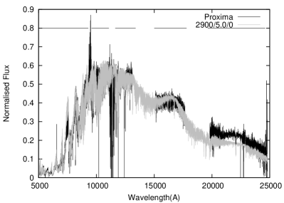
Figure 1: Left: dependence of $S$ on $T_{\rm eff}$ , log g. Right: the best fit of synthetic spectrum 2900/5.0/0 to the observed VLT/X-shooter spectrum of Proxima. We remove here the spectral regions of the strong telluric absorption in J and K bands, spectral ranges used for the fits are indicated by horizontal lines at $F_{\lambda}$ = 0.8.

Rajpurohit et al. (2013) and Passegger et al. (2016) showed that the effective temperature and gravity of normal field M5 dwarfs are $T_{\rm eff}$  = 2900$\pm$100 K and $\log\leavevmode\nobreak\ g$  = 5.0$\pm$0.5, respectively. These values are most likely applicable to Proxima classified as a M5.5 dwarf with solar metallicity. Such metallicity agrees well with the suggestion that Proxima is the third (C) component of the $\alpha$ Cen system, see Reipurth & Mikkola (2012) and references therein.

We fitted our synthetic spectra computed with the Phoenix model atmospheres in the effective temperature $T_{\rm eff}$  range [2600:3100 K] with incremental steps of 100K and gravity $\log\leavevmode\nobreak\ g$  [4.0:5.5] with step 0.5 dex to the observed be VLT/X-shooter  SED. In our work we adopted the ”solar” abundances of Anders & Grevesse (1989), except for iron abundance log N(Fe) = -4.5 in the scale $\sum N_{i}$ = 1.0. These abundances agree with Asplund et al. (2009) within accuracy $\sim$ 0.1 dex for the most elements. Nevertheless, our abundances allow to fit the spectra of the Sun and solar like stars in good agreement with other authors, using comparative simple 1D model atmospheres, see Ivanyuk et al. (2017). We refer the reader to Pavlenko (2014) and Pavlenko & Schmidt (2015) for a review on input data and detailed explanation of the procedure employed to compute the synthetic spectra. Our least squares fitting procedure is described in Pavlenko et al. (2006b). We choose the best fit of the computed spectra to the observed spectrum for the minimum of the $S$ function defined as:

$$S(f_{\rm h},\Delta\lambda,R)=\sum_{\lambda}\left(F_{\lambda}-f_{\rm h}*F_{\lambda}^{s}(\Delta\lambda,R)\right)^{2},$$ (1)

where $F_{\lambda}$ and $F_{\lambda}^{s}$ are the fluxes in the observed and computed fluxes respectively, and $f_{\rm h},\Delta\lambda,R$ are the normalization flux factor, shift in wavelengths between observed and computed spectra, instrumental broadening factor $R$, respectively. We created fits for all synthetic spectra from our grid.

In the left panel of Fig. 1, we show the dependence of $S$ computed for the range of adopted parameters in effective temperature $T_{\rm eff}$  and gravity $\log\leavevmode\nobreak\ g$. We carried out our minimisation procedure only for the ”good”, i.e. without notable telluric absorption and/or emission features across $\lambda\lambda$ 6650 – 6567 Å, 9300 – 9575 Å, 11082 – 11629 Å, 11889 – 11894 Å, 13393 – 15000 Å, 17808 – 19638 Å, see Fig. 1. Shorter wavelengths of $\lambda<$ 5000 Å  were excluded due to some problems discussed in Section 3.1.5. We find a clear minimum of $S$ for $T_{\rm eff}$  = 2900 K for all considered cases of $\log\leavevmode\nobreak\ g$ . The dependence on $\log\leavevmode\nobreak\ g$  is rather weak when varying the $T_{\rm eff}$.

3.1.2 Gravity from absorption lines in NIR VLT/X-shooter spectra of Proxima.

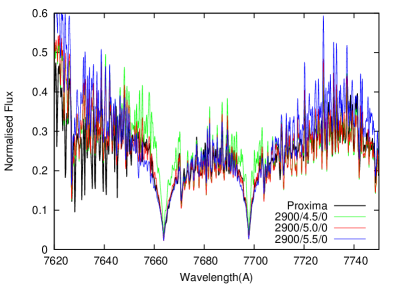
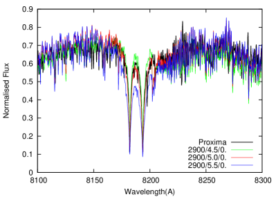
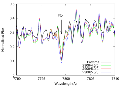
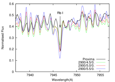
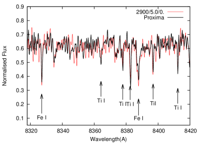
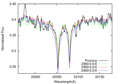
Figure 15: Top panel: fits to the observed KI resonance doublet (left), subordinate triplet of NaI (right). it Middle panel: fits to RbI resonance doublet lines. Bottom panel: fits to the observed profiles of TiI, FeI, and NaI lines.

We showed that the fit to observed SED of Proxima suggests $T_{\rm eff}$  = 2900 K (Fig. 1). To constrain further the gravity of Proxima, we fit gravity-sensitive absorption lines present in the optical spectrum. Here we draw main attention to the profiles of atomic lines. It is worth noting that due to complicatedness of spectra of M-dwarfs the comparison of atomic line profiles in computed and observed spectra is not easy task. The atomic lines in spectra of M-dwarfs form at the background of the haze of molecular lines of different intensity. The molecular features/blends cannot be fitted as good as atomic lines. Nevertheless, comparison of observed and computed profiles of atomic lines allows us to constrain appropriate input parameters. In particular, we focused here our efforts on the resonance lines of potassium at 7664.9 and 7698.96Å as well as the subordinate triplet of sodium at 8126Å, which are well-known gravity indicators. We show the fits to these lines in Fig. 15. We can conclude that the optical spectrum of Proxima is best reproduced with solar abundances and $\log\leavevmode\nobreak\ g$  = 5.0 dex. Our results agrees within the uncertainties with the $\log\leavevmode\nobreak\ g$  = 5.5 dex derived by Passegger et al. (2016).

3.1.3 CO bands

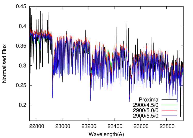
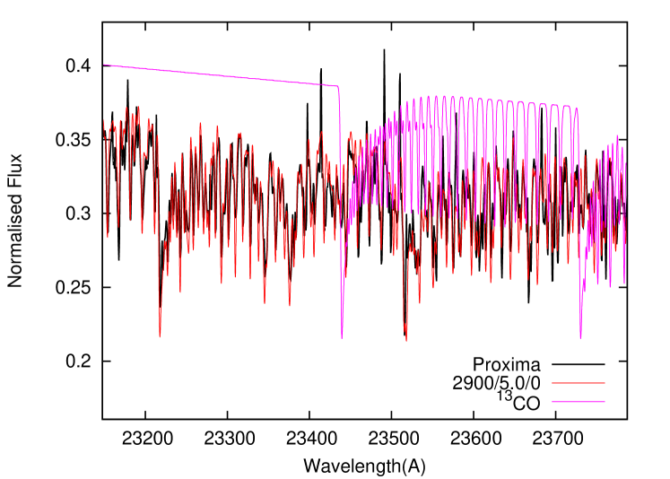
Figure 16: Top: fit of our synthetic spectra governed mainly by ¹²CO bands to the observed VLT/X-shooter  spectrum. Bottom: ¹³CO bands in the theoretical spectrum computed for the parameters of Proxima.

In Fig. 16 we compare the observed spectrum of Proxima with the theoretical spectrum using the $\Delta v$ = 2 CO bands computed for the 2900/5.0/0 model atmosphere. We can see that the fit of the synthetic CO bands to the observed data is a good diagnostic to infer the physical conditions in M dwarf atmospheres, see Pavlenko (2002). In particular we find that the synthetic spectra with the proper effective temperature match reasonably well the observations and agree with the temperatures derived by empirical methods. We see a rather marginal response to a presence of outer hot atmospheric layers, i.e. of a chromosphere, because CO is a very stable molecule of large dissociation potential (D₀ = 11.105 eV). In general, the CO bands are seen in absorption. At the resolution of our observations we may conclude also that our ¹²C/¹³C ratio is consistent with the solar because the ¹³CO bands are weak or even absent in the observed spectrum (Fig.16).

3.1.4 Abundances in the Proxima atmosphere

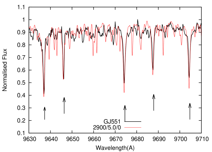
Figure 2: Synthetic fit to Ti I lines marked by arrows in the observed VLT/X-shooter spectrum.

$\lambda$	$gf$	E” (eV)	log N(Ti)
9638.31	2.44E-01	0.848	-7.05 $\pm$  0.15
9647.37	3.68E-02	0.818	-7.05 $\pm$  0.15
9675.54	1.57E-01	0.836	-7.35 $\pm$  0.15
9688.87	2.45E-02	0.813	-7.35 $\pm$  0.15
9705.66	9.79E-02	0.826	-7.20 $\pm$  0.15

Figure 3: Abundances of TiI obtained from the fits to lines shown in Fig. 3.

In the previous sections we analysed the saturated lines of atoms and molecules, which, by definition, show a rather marginal dependence on the changes of abundances. We can assume here that the abundances of the alkali elements shown in Fig. 15 do not differ much from the solar case. In the VLT/X-shooter  spectra we observe also absorption lines of other elements at the background of the local pseudo-continuum formed by the molecular bands across the optical and NIR spectral ranges. Therefore, to make our abundance analysis more reliable, we employ a few atomic lines of intermediate strength present in the red part of the optical spectrum of Proxima where molecular absorption is weaker. We discuss these lines below.

Titanium. Lines of TiI are more numerous than FeI in the spectrum of Proxima due to the lower potential of ionisation of titanium. In Fig. 3 we show the fit with the synthetic spectrum computed for the 2900/5.0 model atmosphere with the solar $\log$ N(Ti) = $-$7.05 (Grevesse & Sauval 1998). In Table 3 we list the derived abundances. We find a Ti abundance of log N(Ti)=-7.20 $\pm$  0.15 from an average of five TiI lines, suggesting a weak metal deficient atmosphere for Proxima. However, we caution this abundance estimate because we see that most of the observed absorption lines are weaker than the lines in the theoretical spectrum computed at solar abundance.

Iron. Iron lines are numerous in the spectrum of Proxima but not as intense as the TiI lines. Although weak lines are more affected by the uncertainties, the theoretical and observed spectra agree qualitatively well as shown in the left panel of Fig. 4. On the right panel of Fig. 4 we display the fit to the observed profile of the intense FeI line at 8327.06Å ($gf$ = 0.02985), showed also in Fig. 15. We obtained good quantitative agreement for $\log$ N(Fe) = $-$4.4 dex, similar to the the solar iron abundance within $\pm$0.2 dex.

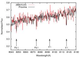
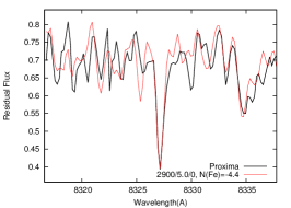
Figure 4: Left: fits to the observed FeI and VI lines with the 2900/5.0/0 model atmosphere. Right: fit to the observed FeI line at 8327.06Å with $\log$ N(Fe) = $-$4.4

Lithium. The absorption bands of the TiO molecule govern the spectra of M dwarfs around the Li resonance doublet at 6707.8Å. The Li doublet is not seen in the spectrum of Proxima as expected for a fully convective old low-mas star. We compare the observed by HARPS and synthetic spectra computed with the 2900/5.0/0.0 model atmosphere and the line lists from Plez (1998) and Schwenke (1998). Generally speaking, Schwenke’s TiO line list allows better to reproduce the shape of the blends across spectral range containing Li doublet. However, in our case we can only place an upper limit to the lithium abundance in the atmosphere of Proxima at $\log$ N(Li) = $-$12.04 dex (right panel in Fig. 5).

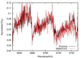
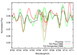
Figure 5: Left: fit to observed fluxes observed across 6708 Å. Right: fits of synthetic spectra computed line lists of Schwenke (1998) and Plez (1998) for different lithium abundances to the observed 6708Å blend, lithium abundances from the bottom: -11.04, -11.54, -12.04…. Model atmosphere 2900/5.0/0.

3.1.5 Atomic and molecular absorption spectra in the 3800–4200Å region

Absorption lines of neutral species in the blue spectra of M-dwarfs are expected to be much stronger than in the solar case due to the lower temperatures and higher pressures in the regions of the absorption line formation. Moreover, we may expect resonance lines of neutral metals to appear due to the changes of their ionisation equilibrium in this low temperature regime.

To verify our treatment of the pressure broadening we compute two spectral regions in the solar spectrum containing rather strong enough lines. We follow the procedure described in Pavlenko et al. (1995) in our computations. The profile of the absorption line is described by a Voigt function $H(a,v)$ and the damping broadening parameter $a$ changes with depth in stellar atmosphere. We computed the synthetic spectra with the VALD3 line list (Ryabchikova et al. 2015; Ryabchikova & Pakhomov 2015) for the 5777/4.44/0 solar model atmosphere (Pavlenko 2003) with a micro-turbulent velocity of $V_{\rm m}$ =1 kms^-1  and wavelength steps of 0.025Å. In Fig. 17 we observe a good agreement between the profiles of strong atomic lines in the observed spectrum of the Sun as a star and the computed spectrum. (Fig. 17).

Figure 6: Identification of absorption lines in the arbitrary selected part in the observed HARPS spectrum of Proxima.

$\lambda$	Element	$gf$	E” (eV)	Visibility
4147.67	FeI	7.87E-03	1.485	Yes
4149.76	FeI	4.93E-06	0.052	Yes
4151.11	Er I	2.73E+00	0.000	Yes
4152.17	FeI	5.86E-04	0.958	Yes
4153.90	FeI	4.77E-01	3.397	No
4154.50	FeI	2.05E-01	2.832	No
4154.81	FeI	3.98E-01	3.368	No
4156.80	FeI	1.55E-01	2.832	No
4159.68	V I	1.86E-02	0.287	Yes

Figure 7: Identification of lines in the HARPS spectrum of Proxima shown in the left panel of Fig.7

We computed the synthetic spectrum of Proxima across the 3800–4200Å wavelength range. Molecular absorption is weak or absent at these wavelengths, implying that we can see deeper layers of the photosphere of Proxima. However, the comparison of the intensities of observed absorption lines compared with the computations reveals reveals some problems here:

• A simple analysis of the lines listed in Table 7 shows that only lines with low excitation energy (E” $<$ 2 eV) are seen in the observed photospheric spectrum of Proxima (Fig. 7). We see that the lines with higher excitation energies are weaker (or even absent) in the observed spectrum.

• The strongest atomic lines in the observed spectrum are much stronger in the synthetic spectra computed in the framework of the classical approach. In other words, damping pressure effects are more pronounced in the computed spectrum where atomic lines have more extended wings.

• Our numerical experiments show that changes of effective temperature by $\pm$200 K or $\log$(g) by $-$0.5 to $-$1.0 do not improve the fit. We cannot reduce the intensities of saturated lines by reducing the associated abundances because we know from the Section 3.1.4 that the metallicity of Proxima is near solar.

We can explain the differences by enhancing the continuum opacity, as shown in Fig. 8 where we compare the observed spectrum with the newly computed one. To reduce the strength of resonance lines we could move the line forming region into lower pressure regions of the atmosphere. In this paper, we use a simple approach suggesting $\chi^{c}_{\nu}=\chi^{c0}_{\nu}\times\kappa$, where $\chi^{c0}_{\nu},\kappa$ are the conventional opacity and adjusting parameter, respectively. Enhancing the continuum opacity across blue spectral range shifts the line forming regions upwards, i.e. to layers of lower pressure. As a consequence, the strongest lines in the computed spectrum show weaker wings, in better agreement with observations. We obtain satisfactory fits after implementing additional continuum opacity in the blue, and can explain the lack of lines of higher excitation potentials, as that case, the photosphere of the star moves upwards into layers of the atmosphere with lower temperature, where only lines of low excitation potential can form. Absorption lines of lower excitation energies form above the ”new” photosphere, making them less sensitive to these changes (Fig. 7).

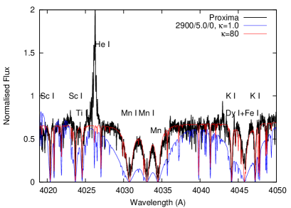
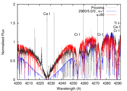
Figure 8: The spectrum of Proxima computed for the model with enhanced continuum opacity across the blue spectral region.

3.2 Emission lines

The intensity of the emission features visible in the spectra changes during the different activity states of the star. To analyse the difference between the typical activity level and the more quiet states we created two average spectra representing the typical active state (S) and the quiet state (QC), see section  2.2. The ’QC’ spectrum shows lower intensity for most of the measured emission lines, specifically the intensity of H$\alpha$ here does not exceed 75% of the maximum emission achieved during strong flares.

3.2.1 Hydrogen Balmer lines

All Balmer lines in the spectrum of Proxima are observed in emission. They show strong variability in time with variations up to a factor of 10 in intensity. As a complementary information, we provide movie with the time variability of the $H_{\alpha}\leavevmode\nobreak\$ in the series of data obtained with HARPS. We measured the pseudo-equivalent widths (pEW) of the emission lines of the full Balmer serie in the VLT/X-shooter spectrum with the task splot under IRAF, which we report in Table 1. Interestingly, measurements of pEW of Balmer lines in the averaged HARPS ’S’ spectrum provides values of the same order than those reported in the Table.

Table 1: Central wavelengths ($\lambda_{c}$) and pseudo-equivalent widths measured on the VLT/X-shooter spectrum and expressed inÅ for the observed Balmer serie

Line	j-i	$\lambda_{c}$	pEW
		Å	Å
H$\alpha$	3–2	6562.797$\pm$0.02	2.5$\pm$0.5
H$\beta$	4–2	4861.323$\pm$0.02	5.1$\pm$0.2
H$\gamma$	5–2	4340.462$\pm$0.02	6.5$\pm$0.5
H$\delta$	6–2	4101.734$\pm$0.02	9.9$\pm$0.2
H$\epsilon$	7–2	3970.072$\pm$0.02	5.4$\pm$1.0
H$\zeta$	8–2	3889.048$\pm$0.02	9.4$\pm$0.8
H$\eta$	9–2	3835.384$\pm$0.02	3.9$\pm$0.1
H$\theta$	10–2	3797.898$\pm$0.02	4.7$\pm$0.4

In Fig. 9 we show the intensity profiles of the H${\alpha}$ line vs Doppler velocity ($V_{\rm r}$  = $\Delta\lambda/\lambda\times c$), where $c$ is the speed of light. We show the profiles for both the quiet (left; QC) and flare (right; S) states. In our spectra we see the full Balmer serie, from the $H_{\alpha}$ line to $H_{\theta}$, corresponding to the 3–2 and 10–2 transitions of the hydrogen atom, respectively. Comparison of their emission profiles provides at least a few important results:

• All Balmer lines show strong variability responding to the temporal changes of flare activity.

• Self-absorption in the core of the $H_{\alpha}\leavevmode\nobreak\$ line is observed practically for all stages of activity of Proxima (see movie³ in supplementary data). We interpret this phenomenon as evidence for the existence of comparatively cool matter outside the flare region. The peak of the line on the red side is higher than on the the blue, most likely due to the outward motion of the neutral hydrogen as discussed in Fuhrmeister et al. (2011).

• The positions of lines do not change during flare events. We interpret this fact as evidence for a quasi-stationary state of the region where Balmer emission lines form.

• The profiles of all Balmer lines in emission in the intensity vs. doppler velocity parameter space have the same FHWM despite of the differences in intensity. The similarity in the profiles of emission lines displayed in Fig. 9 is an evidence that they form in the same region of the atmosphere of Proxima heated by flares.

• Some lines in the Fig. 9 show a well-pronounced peak at $V_{r}$ = – 30 kms^-1 , which we interpret as a indication of an hot stellar wind moving outwards from the star. This peak is well detected in in $H_{\alpha}$ and $H_{\beta}$, and seen as a wide feature in the blue wings of $H_{\gamma}$ - $H_{\epsilon}$.

• In the $H_{\zeta}$ profile, we again see a well-pronounced emission feature at $V_{r}$ = –30 kms^-1 , however, in this case we identify this as He I line at 3889.64 Å, see section 2.

• The component shifted blue-ward does not change much with the activity phase, suggesting that it probably forms in the hot ionized plasma flow (stellar wind) far enough from the flare region of the star.

• When the flare activity rises, the increased emission in $H_{\alpha}\leavevmode\nobreak\$ covers the line in the blue wing (see movie³ in supplementary material). This detail is also seen in Fig. 14 of Fuhrmeister et al. (2011) at lower level activity times.

Photospheric spectrum as well as fluxes show rather marginal responses on the flare activity. In the following we use flux ratios measured in VLT/X-shooter  spectra in combination with measurements of pseudo-equivalent widths of $H_{\alpha}\leavevmode\nobreak\$ and emission feature in its blue wing in the HARPS ’S’ and ’QC’ spectra as shown in Fig. 10.

To determine the $H_{\alpha}$ flux of Proxima received at Earth we followed the procedure by Herbig (1985):

$$f_{H_{\alpha}}=pEW_{H_{\alpha}}\frac{F_{\lambda}(6563)}{F_{\lambda}(5556)}F_{\lambda}(6563,0.0)10^{-0.4V}$$ (2)

where the second term is the average flux ratio at the indicated wavelengths for the star. The third term is the VLT/X-shooter  flux at 6563 Å, received from a star of magnitude $V$ = 0 mag, assumed to be 3.8 10^-9 erg cm^-2 s^-1 Å^-1. Despite of the noise in the X-Shooter spectrum at 5556Å, we estimated the second term from the X-Shooter spectrum and measured a flux ratio of $\frac{F_{\lambda}(6563)}{F_{\lambda}(5556)}$= 3$\pm$2.

The pEW values of 2.7 $\pm$  0.1 and 2.6 $\pm$  0.1Å were determined in ’S’ and ’QC’ spectra, respectively, with the average value of $pEW_{H_{\alpha}}$= 2.65 $\pm$0.1 Å. For a magnitude of $V$ = 11.13 for Proxima (Jao et al. 2014), we derived an average value of $f_{H_{\alpha}}$= 1.07 $\pm$0.7 10^-12 erg cm^-2 s^-1.

In addition, the second term can be estimated from the $R-I$ colour, using the relationship found by Hodgkin et al. (1995)

$$\frac{F_{\lambda}(6563)}{F_{\lambda}(5556)}=2.786(R-I)_{C}-0.932$$ (3)

where $R-I$= 2.04 mag for Proxima (Jao et al. 2014), and $\frac{F_{\lambda}(6563)}{F_{\lambda}(5556)}$= 4.75$\pm$0.03, resulting $f_{H_{\alpha}}$= 1.7$\pm$0.1 10^-12 erg cm^-2 s^-1.

As a final result we adopted the mean value of both measurements, resulting $f_{H_{\alpha}}$= 1.4$\pm$0.4 10^-12 erg cm^-2 s^-1. From this value of $f_{H_{\alpha}}$, we obtained a luminosity in the $H_{\alpha}$ of $L_{H_{\alpha}}$ = 2.8$\pm$0.4 10⁺²⁶ erg s^-1 adopting the distance of 1.30 pc for Proxima from Jao et al. (2014)) and a $L_{H_{\alpha}}$/$L_{bol}$ = 4.5 $\pm$0.4 10^-5 adopting the bolometric luminosity of 6 10⁺³⁰ erg s^-1 from Fuhrmeister et al. (2011).

We determine $pEW_{b}\leavevmode\nobreak\$of the emission feature seen in the blue emission wing of $H_{\alpha}\leavevmode\nobreak\$ at $V_{r}$ =  – 30 kms^-1  in the average HARPS spectrum as shown in Fig. 10, We measure in ’S’ and ’QC’ HARPS spectra $pEW_{b}\leavevmode\nobreak\$= 0.018 Å, the ratio $pEW_{b}\leavevmode\nobreak\$/$pEW_{H_{\alpha}}$ = 0.007. It allows us to estimate the total energy emitted by the stellar wind in $H_{\alpha}\leavevmode\nobreak\$

$$L_{H_{\alpha}}^{b}=7.0\times 10^{-3}\,\times\,2.8\times 10^{26}=\,2.0\times 10^{+24}.$$ (4)

Assuming complete ionisation of hydrogen in the emitting region we determine the number of emitting $H_{\alpha}$ atoms, i.e lower limit of mass loss:

$$\dot{M}=L_{H_{\alpha}}^{b}/h\nu*m_{p}*N_{sec}=3.7*10^{19}g/yr=1.8*10^{-14}M_{\odot}/yr,$$ (5)

where $m_{p}$ and $N_{sec}$ are the mass of H I atom and the number of sec in 1 year.

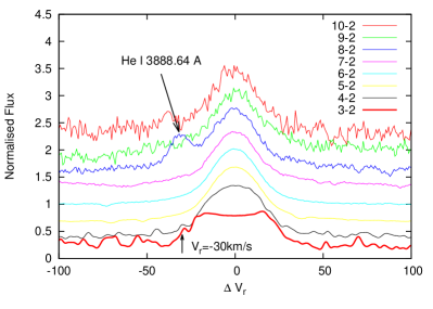
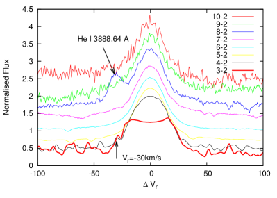
Figure 9: Profiles of Balmer lines shown in the flux normalised to 1.0 in the center of lines vs. radial velocity obtained in quiet mode (left) and flare mode (right). To simplify the plot profiles are shifted in vertical scale, $H_{\alpha}\leavevmode\nobreak\$ is shown by solid line. The arrows mark the positions of the $V_{\rm r}$ = -30 kms^-1  component feature and He I 3888.64Å line.

Figure 10: Scheme of the measurements of the pseudo-equivalent widths of $H_{\alpha}\leavevmode\nobreak\$ and $V_{\rm r}$ = -30 kms^-1  feature in HARPS spectra of Proxima.

3.2.2 HeI line at 4026.19 and 3888.64 Å

The HeI line at 4026.19Å was identified by Fuhrmeister et al. (2011), see their Fig. 13 and Table 2. We observe strong variability of this line in the observed spectra. We note that the HeI line has the highest excitation energy ($E^{\prime\prime}$ = 20.97 eV (see Table 3) with respect to other emission lines observed across our spectral range. It mostly likely formed in the outermost layers of the atmosphere heated by shock waves. Indeed, the HeI cannot be formed in the same place where emissions in the cores of absorption lines of neutral metals form. Furthermore, the HeI emission line is broader.

In the ’QC’ dataset, the HeI line shows multiplet structure and looks more intensive in comparison with S state (Fig 11). We suggest that the strong flares destroy the extended emitted region where the line is formed. Likely, broad component seen in the ’S’ spectrum can be associated with flare region, where, by definition, dispersion of velocities to be larger. In the more quiet modes, we see a few shells moving outwards from the star represented by components equally shifted blue-wards and red-wards suggesting a multi-component for the line, see Table 3.

Other He I line of is seen in the blue wing of hydrogen H_ζ line, at 3888.64 Å. Excitation potential of this line is only a bit lower (19.82 eV) in comparison with 4026Å line, see Table 2. Both lines do not show any remarkable wavelength shift, so we may assume they form in in the same extended quasi stable hot layers.

Table 2: Spectroscopic parameters of the emission HeI lines

Wavelength	Terms	$j^{\prime\prime}$–$j^{\prime}$	$E^{\prime\prime}$ – $E^{\prime}$
(A)			(cm-1)
4026.18436	3Po-3D	2–1	169086.87 – 193917.26
4026.18590	3Po-3D	2–2	169086.87 – 193917.26
4026.18600	3Po-3D	2–3	169086.87 – 193917.25
4026.19675	3Po-3D	1–1	169086.95 – 193917.26
4026.19829	3Po-3D	1–2	169086.95 – 193917.26
4026.35695	3Po-3D	0–1	169087.93 – 193917.26
3888.60467	3S-3Po	1–0	159856.08 - 185564.96
3888.64560	3S-3Po	1–1	159856.08 - 185564.69
3888.64893	3S-3Po	1–2	159856.08 - 185564.67

Table 3: Observed components of the emission HeI 4026Å line

NN	$\Delta\lambda$	$V_{\rm r}$
	(Å)	(kms-1 )
1	$-$0.560	$-$41.73
2	$-$0.420	$-$31.29
3	$-$0.240	$-$17.88
4	$-$0.080	$-$4.59
5	0.090	6.71
6	0.220	16.39
7	0.380	28.32

Figure 11: Profiles of HeI 4026Å line observed in ’S’ and ’QC’ states of flare activity

3.3 Emission cores of resonance lines of atoms and ions

3.3.1 H and K of Ca II

CaII H and K lines are well known as indicators of stellar activity. These lines are collisional controlled and respond to an increase in the temperature of the lower chromosphere of quiet stars like the Sun or Arcturus (Ayres & Linsky 1975). Hence, the appearance of these lines in the spectrum of Proxima is the evidence of chromosphere. Moreover, these lines are extremely strong:

• Emission lines of H and K CaII fill the broad absorption lines seen in less active M dwarfs of the same spectral type, such as GJ699 (Barnard star) as shown in Fig. 12.

• These emission lines do not show any wavelength shift with respect to the photospheric lines.

• The emission profiles of the H and K lines are more intense in the quiet states, in contrary to what we see for Balmer lines of hydrogen. Likely, big flares might affect the regions of their formation.

• The self-absorptions seen in the cores of the CaII H and K lines indicates that the temperature drops at the upper boundary of their formation region.

• The intensity of their components changes in time and with activity, as demonstrated in the movie in the supplementary material.

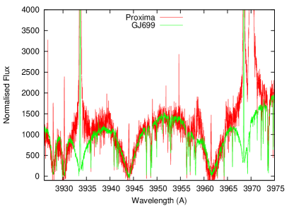
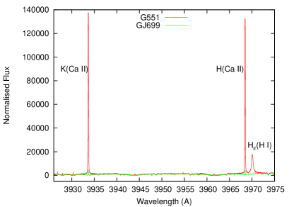
Figure 12: Left: emission lines in the spectral region of the Ca II H and K lines in of the star Proxima and and GJ 699, see section 3.3.2. Right: the same plot shown over a wider wavelength range. The GJ699 spectrum shown here was downloaded from the HARPS archive.

3.3.2 Na H and K resonance lines

Strong emission H and K resonance lines of sodium are notable features in the observed spectra of Proxima. These lines are controlled by photoelectric processes (Thomas 1959). For these lines, the ratio of the photo-ionisation sink to the collisional sink is much larger than 1, see Athay (1972). Therefore, these lines, like the hydrogen lines, show a rather marginal response to the temperature gradients present in chromospheres. We refer the reader to the response of lithium line on chromospheric-like structures in the atmosphere of M dwarfs described in Pavlenko (1998b) . Only extreme cases of chromospheric activity can provide emission cores in the photo-electrically controlled lines, which is most likely the case of Proxima.

In Fig. 13, we compared the profiles of K and H lines of the NaI resonance doublet, which indicate a few non-trivial results:

• The strong emission cores seen in the NaI resonance doublet show significant changes of total emitted energy, see movie.

• However dispersion of velocities in line forming region change very little with the activity level. In the more quiet mode (QC), emission profiles of both components are a bit narrower, while flares increase the width of the emitted lines. Likely, resonance doublet of NaI forms in the chromosphere of the star.

• The profiles of strong photospheric absorption lines practically do not show any response on the level of activity, suggesting that photospheric layers are not bound or weakly bound with regions governed by stellar activity processes.

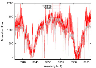
Figure 13: Left: resonance doublet of NaI in different levels of activity. Right: resonance doublet of AlI in comparison with GJ 699, both shown in quiet state.

3.3.3 Other emission lines

In Table LABEL:_other we provide the list of other emission lines with emission cores seen in the spectrum of Proxima. We find emission lines of many different elements, from HeI (z=2) to Dy (z=66). Our list is more complete than the one given in Fuhrmeister et al. (2011) because of the higher spectral resolution of our spectra. Moreover, our list contains both pure chromospheric lines and lines of very high excitation like HeI, which can be formed in areas governed by shock waves (i.e. formed outside the chromosphere). We can distinguish them by the widths of their observed profiles because chromospheric lines formed in the cores of absorption lines are narrower than the lines of hydrogen and helium formed in the layers with larger velocity dispersion.

We assign some specific labels to some of the lines, as follows: – ’ec’ – absorption lines with emission cores,

– ’ecs’ – emission cores with self-absorption as shown in the left panel of Fig. 14,

– P Cyg and iP Cyg - absorption lines with emission components in the red and blue wings, respectively. An inverse P Cyg line is shown in the right panel of Fig. 14.

We generally find that most of the strong resonance lines show emission cores and are often shifted with respect to the central wavelengths. Observed emission cores do not form in the spherically symmetrical and stable atmosphere. Moreover, the strong temporal changes of the emission lines provide evidence that the layers of the chromosphere where they form are strongly affected by the flaring processes. Some other cases show P Cyg or inverse P Cyg profiles. These phenomena likely reflect the complicate dynamical processes occurring in the atmosphere of Proxima.

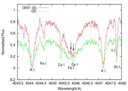
Figure 14: Left: absorption lines of the neutral metals with emission cores. Left arrow at 4045.81Å marks the self-absorption in the core of the strong Fe I absorption line. In the ’S’ spectrum we note the strong emission detail in the core of the nearby Dy I $\lambda$ 4045.97Å line is marked by the right arrow. In the ’QC’ spectrum the detail is ”eaten” by self-absorption. Self-absorption in the weak emission core of K I line at $\lambda$ 4047.21 is seen as well. Right: example of iP Cyg profiles.

4 Discussion on the atmosphere of Proxima

4.1 Photosphere

Analysis of the VLT/X-shooter spectra obtained with intermediate resolution showed that the atmosphere of Proxima in the optical and near IR spectral range is similar to the rest of normal M-dwarfs of the same spectral classes M5-M6. The optical spectral range is governed by Ti and VO bands, molecular bands of water dominates in the near IR. Our theoretical spectra computed for a model atmosphere of $T_{\rm eff}$  = 2900 K fits well enough the observed spectral energy distribution in accordance with results of Rajpurohit et al. (2013) and Passegger et al. (2016). In summary, we obtain rather good fits of our synthetic spectra computed for the canonical PHOENIX model atmosphere of solar metallicity across all spectral ranges observed by VLT/X-shooter , except for slightly lower fluxes in the spectral region of the K-band, which seems to be a common problem of similar mid M-dwarf investigations, see Pavlenko et al. (2006a).

Our computed spectral energy distributions depend on log g rather marginally, still we note a weak trend toward lower log g in accordance with $\log\leavevmode\nobreak\ g$ = 4.5 found by Mann et al. (2015). On the other hand, strong alkali lines provide clear response on log g changes. We obtained better fits to profiles of some observed absorption lines of Na, Rb, subordinate triplet of Na at 8200Å with log g = 5.0, see also Rajpurohit et al. (2013), instead of log g = 5.5, as obtained by Passegger et al. (2016). Our result is in agreement with the log g = 5.23 $\pm$  0.14 derived from the interferometric measurement of the Proxima radius and mass-radius relations (Demory et al. 2009).

The opacity of TiO bands around 4200Å starts to decrease bluewards (Pavlenko 2014). At shorter wavelengths, we explore deeper regions of the atmosphere of Proxima, where the observed spectrum is dominated by absorption lines of neutral atoms. The resonance lines of neutral species become very strong. Theoretical spectra provide too strong wings due to the effects of pressure damping which broadens these lines. In the case of Proxima we obtain the best solution for $\kappa$ = 80. This value looks very high, but we work in the regime of low temperatures where the conventional opacity is extremely low in this case due to the low density of the $H^{-}$ ion, which is the main source of opacity in the atmospheres of M stars. In other words, we should find larger electron densities to increase opacity in the low photospheric layers. We suggest that this effect may be created by the over-ionisation of alkali metals which are the main donors of free electrons. Indeed, photons with $\lambda<$ 4200Å can ionise the neutral atoms in late-type atmosphere due to the low electron densities where processes of recombination are not so effective. The additional opacity affects only the emitted spectrum in the UV and blue wavelengths, occurring deep in the atmosphere. The temperature structure of the upper layers of the model atmosphere are mainly determined by molecular opacities, which explain why we can reliably fit the spectral energy distribution of Proxima at longer wavelengths.

On the other hand, for some spectral diagnostics, it could also be that the analysis is too simplified and 1-D LTE syntheses may indeed underestimate some of the opacity (lines) in the blue. More complex analysis involving 3-D atmospheres from hydro simulations sometimes find that the missing opacity is even larger in 3D NLTE models than in 1-D LTE. There are hints in the paper by Fuhrmeister et al. (2011) that much more sophisticated 3-D atmospheres should be applied in the case of Proxima.

4.2 Chromosphere

The chromosphere represents the extended part of the atmosphere of Proxima, where narrow emission lines of different intensities vary with time. We observe temporal variations of these lines because of interactions between the flares and the chromosphere. We know that solar flares originate in high chromosphere-corona regions. The strongest flares move downwards to get deeper into the photosphere. However, our movies show mainly temporal changes of intensity of chromospheric lines, while the photospheric spectrum shows marginal response to flares. In the most cases, even the strongest flares seem to occur in local regions far above the surface/photosphere of Proxima. The TiO line forming region is separated from the hot flare regions by the mantle of the cool plasma. Nevertheless, the chromosphere of Proxima is very powerful because it shows many absorption lines of neutral metals with narrow emission cores. These emission cores most likely form in the chromosphere, above the temperature minimum. The presence of emission cores within the lines of neutral alkalies and neutral atoms which are fully controlled by radiation can only occur in the presence of steep temperature gradients in the chromosphere, see e.g. NLTE simulations of emission cores of Li in Pavlenko (1998a).

4.3 Flares

Hydrogen Balmer lines in emission is a common phenomenon in the Sun. Balmer lines are controlled by photo-electrical processes and are not sensitive to the temperature structure of the atmosphere. Their emission is mainly the result of ionization and collisional processes created by shock waves following flare event. The Hydrogen emission lines seen in the Proxima spectrum form mainly in flare regions. They are broader than chromospheric lines of CaII, NaI and other neutral metals. This effect most likely results from a larger scatter in their velocity distribution, as seen in Fig. 12, where we compare the CaII and H_ϵ lines: the CaII is much stronger, but H_ϵ is broader.

4.4 Stellar wind

We observe a quasi-stationary component in the blue wing of the $H_{\alpha}\leavevmode\nobreak\$ and $H_{\beta}$ emission in the HARPS spectra. We interpret its presence as a result of the flow of highly ionized plasma with a velocity of $V_{r}$ = $-$30 kms^-1 . We assume that the observed component most likely relates to the the hot stellar wind outflow generated by the high level of flare activity in Proxima. From our estimate of the total energy emitted in the $H_{\alpha}$ line, we infer a lower limit of the mass loss of $\dot{M}=1.8\times 10^{-14}M_{\odot}/yr$ because we do not consider emitted energies by other emission lines.

Wood et al. (2000, 2001) estimated a four or six times lower mass loss of $\dot{M}\leq 0.2\dot{M}_{\odot}$ = 0.5 10${}^{-14}M_{\odot}/yr$ or 0.3 10${}^{-14}M_{\odot}/yr$ for the cases of average solar wind mass loss $\dot{M_{\odot}}$ = 1.374 10¹² g/sec = 2.3 $10^{-14}M_{\odot}/yr$ (Hundhausen 1997) and $\dot{M_{\odot}}\sim 1.3\leavevmode\nobreak\ 10^{-14}M_{\odot}/yr$ (Goldstein et al. 1996), respectively. Nevertheless, measurements by Wood et al. (2000, 2001) are based on the analysis of the $L_{\alpha}$ absorption which relates to absorption by neutral hydrogen atoms. Both estimates relate to different parts of the stellar wind. It is worth noting that the level of activity and, respectively, mass loss for the late type stars should change in time. Indeed, we observe different levels of activity in the M-dwarfs population of our Galaxy. The spectrum of GJ699 used in our paper for the comparison with Proxima provides clear evidences of much lower level of activity. Likely, nowadays Proxima passes its evolutionary epoch of high activity.

In our spectra we see manifestations of cool and hot components of the stellar wind from Proxima. Cool neutral hydrogen located above the flare region provides the asymmetrical self-absorption in $H_{\alpha}\leavevmode\nobreak\$ core, as discussed in Fuhrmeister et al. (2011). We defer a more detailed analysis of this phenomenon to a future paper.

5 Conclusions

In the framework our work at least a few results were obtained:
$\bullet$ From the fits spectral energy distributions observed in the optical and near infrared spectral ranges we obtained effective temperature of Proxima   $T_{\rm eff}$  = 2900 $\pm$  100 K.
$\bullet$ Fit to profiles of strong atomic lines atomic lines observed in the optical spectrum of Proxima provides good restriction for the gravity in atmosphere $\log\leavevmode\nobreak\ g$ = 5.0 $\pm$  0.25.
$\bullet$ From the analysis of strong resonance and subordinate lines of Na, K, Rb as well as lines of intermediate strengths of Ti I and Fe I lines formed at the background of TiO and VO bands we obtain solar abundances of these elements in the atmosphere of Proxima.
$\bullet$ From the fits to the observed spectrum across Li resonance doublet we determined the upper limit of Li abundance log N(Li) = $-$12.04, which is consistent with the expected depletion of an old fully convective low-mass star.
$\bullet$ Photospheric lines observed in the optical and infrared spectra of Proxima can be fitted by standard synthetic models. However observed strong lines of low excitation potentials in the blue spectral region show narrower profiles than expected indicating a formation in lower pressure layers in the atmosphere. We were able to reproduce their profiles incorporating additional opacity, which shifts their formation layers upwards, in the lower pressure regions.
$\bullet$ In spite of a comparatively high level of activity we found that the photospheric spectrum show rather marginal response on the flare activity of Proxima, except for very strong flares.
$\bullet$ The emission lines of hydrogen are good indicators of stellar activity. At the times of strong flares they become more intense. On the contrary, strong emission lines formed in the chromosphere, i.e., H&K Ca II, H&K Na I, reduce their intensity at the occurrence of strong flares. Likely strong flares change the structure of chromosphere. These chromospheric originated lines are narrower in comparison with hydrogen lines formed in the flare region.
$\bullet$ The He I line at 4026.19Å is observed in emission and reduces its intensity in the presence of strong flares,too. Due to the larger excitation potential of the He I line, it should form in hotter layers above the hydrogen lines formation region. In the absence of strong flares the He I emission line at 4026.19Å shows multicomponent profile. Likely, it reflects complicate structure of the line forming region. In the ’S’ spectrum the intensity of the He I lines is lower than in QC, it means that the He I lines formation layers are affected by flares.
$\bullet$ In the blue wing of emission hydrogen $H_{\alpha}\leavevmode\nobreak\$ and $H_{\beta}$ lines we found an emission component shifted to $V_{\rm r}$ = 30 kms^-1  with respect to their cores. We interpret the emission components as evidence of the hot stellar wind from Proxima. Using the simple model of complete ionisation of hydrogen atoms in the stellar wind we estimate a minimum mass loss of $\dot{M}$ = 1.8 10${}^{-14}M\odot/yr$.

Appendix A

Figure 17: Comparison of the strong lines in the spectrum of the Sun as a star Kurucz et al. (1984) and the theoretical spectrum computed for 1D model atmosphere of $T_{\rm eff}$ /$\log\leavevmode\nobreak\ g$ /[Fe/H] = 5777/4.44/0.0.

Table 4: Emission lines in Proxima spectrum, see section3.3.3

$\lambda$	Element	$gf$	E” (eV)		Remarks
3819.57	Cr I	1.16E+00	2.708	S,QC	ecs
3824.44	FeI	4.35E-02	0.0	S,QC	ec
3829.36	Mg I	5.93E-01	2.709	S,QC	ec
3832.30	Mg I	1.33E+00	2.712	S,QC	ec
3837.60				S,QC
3838.29	Mg I	2.50E+00	2.717	S,QC	ec
3840.75	V I	7.28E-01	0.040	S,QC	ecs
3847.33	V I	8.51E-02	0.017	S, QC	ecs, P Cyg?
3853.88				S,QC
3856.37	FeI	5.18E-02	0.052	S,QC	ec
3859.91	FeI	1.95E-01	0.000	S,QC	ec
3864.10	Mo I	9.77E-01	0.000	S	ec, iP Cyg?
3870.91				S$>$QC
3872.50	FeI	1.18E-01	0.990	S,QC	ec
3878.57	FeI	4.18E-02	0.087	S,QC	ec
3886.28	FeI	8.39E-02	0.052	S,QC
3887.05	FeI	7.18E-02	0.915	S,QC
3888.66	HeI			S,QC
3894.03	Cr I	2.24E-02	0.961	S,QC	ec
3894.08	Co I	1.26E+00	1.049	S,QC	ec
3894.98	Co I	3.98E-02	0.629	S,QC	ec
3895.66	FeI	2.14E-02	0.110	S,QC	ec
3897.88	FeI	1.84E-01	2.692	S,QC	iP Cyg
3899.71	FeI	2.94E-02	0.087	S,QC	ecs
3903.16	Cr I	5.89E-03	0.968	S,QC	ec
3903.90	FeI	1.57E-01	2.990	QC
3905.52	Si I	9.10E-02	1.909	S,QC
3906.48	FeI	5.71E-03	0.110	S,QC	ecs
3907.49	sr I	2.28E+00	0.000	S,QC	ec
3907.93	FeI	7.64E-02	2.759	S,QC	ec
3908.76	Cr I	8.91E-02	1.004	S	ec shifted to red
3909.86	V I, Co I	7.94E-02	0.069	S,QC	complicate blend
3920.26	FeI	1.80E-02	0.121	S,QC	ecs shifted to red
3922.91	FeI	2.23E-02	0.052	S,QC
3926.82				S,QC	esc
3927.92	FeI	3.01E-02	0.110	S,QC	ec
3930.30	FeI	3.23E-02	0.087	S,QC	ec
3939.26				S	iP Pyg
3940.88	FeI	2.51E-03	0.958	S,QC	ec shifted to blue
3941.49	Cr I	4.07E-02	1.030	S,QC	ec shifted to blue
3941.73	Co I	9.33E-03	0.432	QC	ecs
3944.01	Al I	2.38E-01	0.000	QC,S	ecs
3948.67	TiI	3.98E-01	0.000	S,QC	ec
3960.05				S
3961.52	Al I	4.75E-01	0.014	QC,S	ecs
3983.13				QC,S
4001.66	FeI	1.26E-02	2.176	QC,S	ec blue shifted
4021.87	FeI	1.87E-01	2.759	QC,S	ec
4026.19				QC,S	He II
4030.75	Mn I	3.21E-01	0.0	QC,S	ecs
4032.98	Ga I	2.36E-01	0.0	S
4033.06	Mn I	2.27E-01	0.0	QC,S	ecs
4034.48	Mn I	1.44E-01	0.0	QC,S	ecC
4042.93				QC,S
4044.14	19.00	1.20E-02	0.000	QC,S	P Cyg
4045.97	Dy I	7.08E+00	0.0	S	ec
4047.21	K I	6.03E-03	0.0	QC,S	ecs
4052.96				QC,S
4062.44	FeI	1.37E-01	2.845	QC,S	ecs
4063.59	FeI	1.15E+00	1.557	QC	ecs
4064.21	TiI	1.20E-01	1.053	QC,S	ec
4071.74	FeI	9.51E-01	1.608	QC,S	P Cyg
4077.36	Y I	1.89E+00	0.0	QC,S	iP Cyg
4077.71	Sr II	1.47E+00	0.0	QC,S	P Cyg
4103.94				QC,S
4111.14				na? P Cyg, ecs
4115.18	V I	1.18E+00	0.287	QC,S	ec
4116.47	V I	4.90E-01	0.275	QC,S ec
4116.56	V I	1.47E-01	0.262	QC,S	ec
4131.99	V I	8.51E-01	0.287	QC,S	$-$30 kms-1  emission. iP Cyg.
4132.06	FeI	2.11E-01	1.608	QC,S	the same
4134.48	V I	5.94E-01	0.301	QC,S	ecs
4158.62 ?				QC,S	O II?
4158.67 ?				QC,S	O II?
4159.68	V I	1.86E-02	0.287	QC,S	ec redshifted.
4164.658	Nb I	7.413E-01	0.049	QC,S	in -30 kms-1  emission line
4167.270	Gd I	1.542E-01	0.124	QC,S	P Cyg?
4169.877	Ce II	4.467E-01	0.536	QC,S	P Cyg?
4173.44				QC,S	iP Cyg
4178.85				QC,S	forbidden FeI?
4181.93				QD,S
4184.07				QD,S
4185.15				QD,S	S
4191.09				QD,S	S
4198.30	FeI	1.91E-01	2.399	QC $>$ S	P Cyg
4200.7				QC $>$ S	nebular?
4215.52	Sr II	7.16E-01	0.0	QC,S
4216.18	FeI	4.41E-04	0.0	QC,S	ec shifted blueward.
4226.73	Ca I	1.75E+00	0.0	QC,S	ecs shifted to the red
4227.43	26.00	1.84E+00	3.332	QC,S	P Cyg
4233.15				QC,S
4237.27				QC,S
4254.35	Cr I	8.13E-01	0.000	QC,S
4259.31	V I	6.76E-03	0.017	QC,S	P Cyg
4266.34				QC,S
4272.23				QC,S
4274.81	Cr I	6.03E-01	0.0	QC,S	ec
4277.538	TiII	1.816E-01	4.969	QC,S	P Cyg
4289.73	Cr I	4.27E-01	0.0	QC,S	ec
5889.95	Na I	1.28E+00	0.0	QC,S	ecs
5895.92	Na II	6.40E-01	0.0	QC,S	ecs