Gene Hunting with Knockoffs for Hidden Markov Models

Abstract

Modern scientific studies often require the identification of a subset of relevant explanatory variables, in the attempt to understand an interesting phenomenon. Several statistical methods have been developed to automate this task, but only recently has the framework of model-free knockoffs proposed a general solution that can perform variable selection under rigorous type-I error control, without relying on strong modeling assumptions. In this paper, we extend the methodology of model-free knockoffs to a rich family of problems where the distribution of the covariates can be described by a hidden Markov model (HMM). We develop an exact and efficient algorithm to sample knockoff copies of an HMM. We then argue that combined with the knockoffs selective framework, they provide a natural and powerful tool for performing principled inference in genome-wide association studies with guaranteed FDR control. Finally, we apply our methodology to several datasets aimed at studying the Crohn’s disease and several continuous phenotypes, e.g. levels of cholesterol.

Keywords. Markov chains, hidden Markov models, model-free knockoffs, knockoff filter, exchangeable random variables, false discovery rate, controlled variable selection, genome-wide association studies.

1 Introduction

1.1 The need for (more) controlled variable selection

The automatic selection of relevant explanatory variables is a fundamental challenge in statistics. Its urgency is induced by the growing reliance of many fields of science on the analysis of large amounts of data. As researchers are striving to understand increasingly complex phenomena, the technology of high throughput experiments now allows them to measure and simultaneously examine millions of covariates. However, despite the abundance of the available variables, it is often the case that only a fraction of them are expected to be relevant to the question of interest. By discovering which are important, scientists can design a more targeted followup investigation and hope to eventually understand how certain factors influence an outcome. A compelling example is offered by genome-wide association studies (GWAS): here, the goal is to identify which markers of genetic variation influence the risk of a particular disease or a trait, choosing from a pool of hundreds of thousands to millions of single-nucleotide polymorphisms (SNP).

In general, a good selection algorithm should be able to detect as many relevant variables as possible using only a small number of samples ($n\ll p$), since these tend to be expensive to acquire. At the same time, it should be sufficiently cautious to ensure that the findings are replicable and not just report spurious correlations or associations. Several statistical techniques have been proposed in an effort to address and balance these two conflicting needs. The standard approach adopted in GWAS consists in controlling the global error when testing a large collection of hypotheses, each probing the effect of one of the typed genetic markers on the phenotype of interest. A p-value for the null hypothesis of no association between a genetic variant and the outcome of interest is obtained using linear models (or generalized linear models for binary traits) with one fixed effect (the genotype of the variant) and possibly random effects capturing the contribution of the rest of the genome. To identify significantly associated variants, the p-values are compared to a threshold that guarantees approximate control of the family-wise error rate (FWER, i.e. the probability of committing at least one type-I error, across all tests) at the 0.05 level (the standard choice is to perform all individual tests at level $\alpha<5\cdot 10^{-8}$).

As it is generally the case, choosing to control the FWER leads to a very conservative selection of relevant polymorphisms. Indeed, it has been observed that the variants identified via this strategy—while apparently reproducibly associated with the traits—can typically only explain a small portion of the genetic variance in the phenotype of interest [1]. An alternative criterion to evaluate statistical significance is the false discovery rate (FDR) [2]. The FDR is a particularly attractive concept when one expects a multiplicity of true discoveries. This has led to its adoption in studies involving gene expression and many other genomic measurements [3], including the study of expression quantitative trait loci (eQTL). A broader adoption of the FDR has been advocated as a natural strategy to improve the power of GWAS [4, 3, 5] for complex traits.

Controlled variable selection is an inherently difficult task in high dimensions, but GWAS present at least two specific challenges. First, many polygenic phenotypes depend on the genetic variants through mechanisms that are mostly unknown [6] and may involve the interaction of different genetic polymorphisms [7]. Unfortunately, the current analysis methods neglect the possibility that the response depends on the explanatory variables in a non linear fashion and through complicated interactions. Clearly, methods based on marginal testing are ill-equipped to detect interactions and the few approaches that simultaneously analyze the role of multiple variants rely on strong linearity assumptions. The second prominent obstacle arises from the presence of correlations among the covariates. The expression linkage disequilibrium is used in genetics to indicate the tight dependence between the alleles at polymorphisms that occupy nearby positions in the genome. This association is due to the process with which the DNA is transmitted in humans and it is a fundamental characteristics of the explanatory variables in GWAS. Methods aiming for valid inference in this settings should certainly take it into account.

These issues motivate the need for the development of new statistical methodologies that can identify important variables for complex phenomena, while providing rigorous guarantees of type-I error control under milder and well-justified assumptions.

1.2 The assumptions of model-free knockoffs

Model-free knockoffs, recently introduced in [8], partially address the aforementioned issues by taking a radically different path from the traditional literature on high-dimensional variable selection. They provide a powerful and versatile method that enjoys rigorous FDR control, under no modeling assumptions on the conditional distribution $F_{Y|X}$ of the response $Y$ given the covariates $X$. In fact, $F_{Y|X}$ may remain completely arbitrary and unspecified. The suprising result is achieved by considering a setting in which the distribution $F_{X}$ of the covariates is presumed to be known. When this is the case, the latter can be used to generate appropriate “negative control” variables (the knockoff copies). These knockoffs are created independently of the measured outcome and they allow to distinguish the relevant from the unnecessary variables. As a consequence, it becomes possible to estimate and, further, control the FDR.

In many circumstances, the premises of model-free knockoffs can be argued to be more principled than those of its traditional counterparts. Intuitively, it is reasonable to shift the central burden of assumptions from $F_{Y|X}$ to $F_{X}$, since the former is the essentially the object of inference. In a GWAS, an agnostic approach to the conditional distribution of the response is especially valuable, due to the possibly complex nature of the relations between genetic variants and phenotypes. Moreover, the presumption of knowing $F_{X}$ is well grounded. On the one hand, geneticists have at their disposal a rich set of models for how DNA variants arise and spread across human populations over time. On the other hand, genome-wide variation has been assessed in large collections of individuals: the UK Biobank (http://www.ukbiobank.ac.uk) contains the genotypes of 500,000 subjects, the RPGEH (https://www.dor.kaiser.org/external/DORExternal/rpgeh/index.aspx) has similar information for over 100,000 individuals, and hundreds of thousands of additional samples are available via dbGaP (https://www.ncbi.nlm.nih.gov/gap), to cite a few examples. The combination of theoretical understanding and data gives us a good handle on $F_{X}$.

In general, the fundamental difficulty with the method of model-free knockoffs is related to the construction of those knockoff copies. This task requires knowledge of the underlying distribution of the original variables, which can rarely be expected to be accessible exactly. In some cases a good approximation is available, but a separate computational issue emerges. Even if the true $F_{X}$ were known, it may still be unfeasible to create the knockoff copies required by this procedure. Until now, the only special case for which an algorithm has been developed is that of multivariate normal covariates [8]. In this sense, model-free knockoffs have not yet fully resolved the second crucial difficulty of GWAS that we mentioned earlier. A multivariate normal approximation cannot fully take advantage of the precious prior information that we have on the sequential structure of allele frequencies across SNPs [9]. It thus seems important to develop new techniques that can exploit some of the advances in the study of linkage disequilibrium and population genetics, and exploit accurate parametric models for $F_{X}$.

1.3 Our contributions

In this paper, we introduce a new algorithm to sample knockoff copies of variables distributed as a hidden Markov model (HMM). To the best of our knowledge, this result is the first extension of model-free knockoffs beyond the special case of a Gaussian design and it involves a class of covariate distributions that is of great practical interest. In fact, HMMs are widely employed in a variety of fields to describe sequential data with complex correlations.

While many applications of HMMs are found in the context of speech processing [10] and video segmentation [11], their presence has also become nearly ubiquitous in the statistical analysis of biological sequences. Important instances include protein modeling [12], sequence alignment [13], gene prediction [14], copy number reconstruction [15], segmentation of the genome into diverse functional elements [16] identification of ancestral DNA segments and population history [17, 18, 19]. Of special interest to us, following the empirical observation that variation along the human genome could be described by blocks of limited diversity [20], HMMs have been broadly adopted to describe haplotypes—the sequence of alleles at a series of markers along one chromosome. The literature is too extensive to recapitulate: we simply recall that taking the move from some initial formulations [21, 22, 23, 24], there are now a vast set of models and algorithms that are used routinely and effectively to reconstruct haplotypes (phase) and to impute missing genotype values. Some of the most common software implementations include fastPHASE [25], Impute [26, 27], Beagle [28, 29], Bimbam [30] and MaCH [31]. The success of these algorithms in reconstructing partially observed genotypes can be tested empirically and their realized accuracy is a testament to the fact that HMMs offer a good phenomenological description of the dependence between the explanatory variables in GWAS.

By developing a knockoff contruction for HMMs, we can incorporate the prior knowledge on patterns of genetic variation. As a result, we obtain a new variable selection method that addresses all the critical issues of GWAS discussed in Section 1.1 and enjoys:

1. Agnostic conditional characterization of the response given the covariates. As in the general model-free knockoff framework, no assumptions are made here. We are completely free from the rather questionable restrictions of linear models and other parametric alternatives.

2. Principled description of the distribution of the covariates. A sensible model inspired by prior scientific knowledge naturally deals with the correlations across SNPs.

3. Powerful performance inherited from the framework of model-free knockoffs. Sophisticated machine learning tools can be used to assess variable importance, without losing any control over the FDR. In addition, any side information about the likelihood of $Y$ given $X$ can be leveraged to improve power.

4. Computationally efficient construction of knockoff copies, derived from the mathematically amenable properties of hidden Markov models. The complexity of the entire procedure can be shown to be $O(np)$.

1.4 Related works

This paper is most closely related to [8], which has introduced the framework of model-free knockoffs. Their work focuses on the special case of multivariate Gaussian variables, while ours extends their results to HMMs. On the other hand, earlier instances of the knockoff method [32, 33] are focused on the linear regression problem with a fixed design matrix.

Traditional multivariate variable selection techniques have been applied in GWAS on numerous occasions. Some works have employed penalized regression, but they either lack type-I error control [34, 35] or require very restrictive modeling assumptions [5]. Similarly, their Bayesian alternatives [36, 37] do not provide finite-sample guarantees. Some have tried to control the type-I errors of standard penalized regression methods through stability selection [38], but they have observed that the resulting procedure does not correctly account for variable correlations and is less powerful than marginal testing. Others have employed non-parametric machine learning tools [39] that can produce variable importance measures, but no valid inference. In theory, some inferential guarantees have been obtained for the Lasso [40, 41], GLMs [42] and even random forests [43], but they only hold under rather stringent sparsity assumptions.

Hidden Markov models have appeared before as part of a variable selection procedure for GWAS, in order to combine marginal tests of association from correlated SNPs [44, 45]. However, this approach is fundamentally different from ours, since it is neither multivariate nor model-free.

2 Model-free controlled variable selection via knockoffs

2.1 Problem statement

The controlled variable selection problem can be naturally stated in formal terms by adopting the general setting of [8]. Suppose that we can observe a response $Y\in\mathbb{R}$ and a vector of covariates $X=(X_{1},\ldots,X_{p})\in\mathbb{R}^{p}$. Given $n$ such samples $(X^{(i)},Y^{(i)})_{i=1}^{n}$ drawn from a population, we would like to know which variables are associated with the response. This can be made more precise by assuming that

$$(X^{(i)},Y^{(i)})\overset{\mathrm{i.i.d.}}{\sim}F_{XY},\qquad i\in\{1,\ldots,n\},$$

for some joint distribution $F_{XY}$. Here, the concept of a relevant variable can be understood by first defining its opposite. We say that $X_{j}$ is null if and only if $Y$ is independent of $X_{j}$, conditionally on all other variables $X_{-j}=\{X_{1},\ldots,X_{p}\}\setminus\{X_{j}\}$. This uniquely defines the set of null variables $\mathcal{H}_{0}=\{j:X_{j}\text{ is null}\}$ and its complement $\mathcal{S}=\{j:X_{j}\text{ is relevant}\}=\{1,\ldots,p\}\setminus\mathcal{H}_{0}$. Our goal is to obtain an estimate $\hat{\mathcal{S}}$ of $\mathcal{S}$, while controlling the false discovery ratio, that is now defined as:

$$\text{FDR}\mathrel{\vbox{\hbox{\scriptsize.}\hbox{\scriptsize.}}}=\mathbb{E}\left[\frac{|\hat{S}\cap\mathcal{H}_{0}|}{|\hat{S}|}\right].$$

We emphasize the natural logic of this definition: a variable is null if it has no predictive power whatsoever once we take into account all the other variables; i.e. it does not influence the response in any way. To relate this with model-based inference, [8] shows that in a logistic model, being null is equivalent—under an extremely mild condition—to saying that the corresponding regression coefficient vanishes.

2.2 The method of knockoffs

The main idea of the model-free knockoffs methodology [8] is to generate a new set of artificial covariates, the knockoff copies of $X$, so that they have the same structure as the original ones but are known to be null. These can then be used as “negative controls” to estimate the FDR with almost any variable selection algorithm of choice. Model-free knockoffs can thus be seen as a versatile wrapper that allows one to extend rigorous statistical guarantees, under very mild assumptions, to powerful practical methods that would otherwise be too complex for a traditional theoretical analysis. A detailed description of this procedure would fall outside the scope of this paper, but we nonetheless begin with a brief summary because our work builds upon this and extends its applicability.

Knockoff variables. For each variable $X_{j}$, suppose that we can construct a knockoff copy $\tilde{X}_{j}$ in such a way that the original variables $X=(X_{1},\ldots,X_{p})$ and their knockoffs $\tilde{X}=(\tilde{X}_{1},\ldots,\tilde{X}_{p})$ satisfy the following two conditions:

$$\tilde{X}\rotatebox[origin={c}]{90.0}{$\models$}\,Y|X,$$ (1)

and

$$\left(X,\tilde{X}\right)_{\text{swap}(S)}\overset{d}{=}\left(X,\tilde{X}\right)\qquad\text{for any }S\subset\{1,\ldots,p\}.$$ (2)

Above, $(X,\tilde{X})_{\text{swap}(S)}$ denotes the vector produced by swapping the entries $X_{j}$ and $\tilde{X}_{j}$, for each $j\in S$. The pairwise exchangeability condition in (2) requires the distribution of $(X,\tilde{X})$ to be invariant under this transformation. This property is essential and we will discuss later how it is not always easy to obtain a non-trivial vector $\tilde{X}$ that satisfies it. We refer to the other (1) as the nullity condition, since it immediately implies that all knockoffs are null. This clearly holds whenever $\tilde{X}$ is constructed without looking at $Y$ and is necessary for the knockoff copies to be used as negative controls.

Feature importance measures. Once the knockoff copies of $X$ are created, one proceeds by computing two vectors of “feature importance statistics”: $T=(T_{1},\ldots,T_{p})$ and $\tilde{T}=(\tilde{T}_{1},\ldots,\tilde{T}_{p})$. For each $j$, $T_{j}$ and $\tilde{T}_{j}$ measure the importance of $X_{j}$ and $\tilde{X}_{j}$, respectively, in predicting $Y$. These can be estimated in almost any arbitrary way from the available data. As an example, we can think of letting $T_{j}$ and $\tilde{T}_{j}$ be the magnitude of the Lasso coefficients for $X_{j}$ and $\tilde{X}_{j}$, obtained by regressing $Y$ on $(X,\tilde{X})$. However, this is just the simplest example from a multitude of potentially more powerful alternatives. Nothing prevents us from computing our estimates by exploiting some form of cross-validation, applying boosting, training a random forest or even a neural network. The only constraint is that $X$ and $\tilde{X}$ should always be treated “fairly”, i.e. disregarding which one is a knockoff and which one is not. In mathematical terms, we say that swapping any subset $S$ of the original variables with their knockoff copies should have the only effect of swapping the corresponding elements of $T$ with $\tilde{T}$.

The knockoff filter. The estimated importance measures of the original variables are then compared to those of their corresponding knockoff copies. If $X_{j}$ is truly relevant, one would expect $T_{j}$ to be larger than $\tilde{T}_{j}$. Conversely, they will tend to behave similarly when $X_{j}$ is null. Formally, one calculates statistics $W_{j}=w_{j}(T_{j},\tilde{T}_{j})$, for some anti-symmetric function $w_{j}$. Properties (1) and (2) imply that all the null $W_{j}$ satisfy the flip-sign condition required to apply the knockoff filter of [32]. Finally, the latter selects a set $\hat{\mathcal{S}}$ of relevant variables while controlling the FDR at the desired target level $\alpha$.

2.3 Constructing knockoffs

Fundamental ingredients of the knockoff method are, of course, the artificial variables $\tilde{X}$. In Section 2.2 we saw that they need to obey the pairwise exchangeability (1) and strong nullity (2) properties, but we have not discussed how to construct them. A possible direction is suggested by the Sequential Conditional Independent Pairs (SCIP) “algorithm” in [8]. For any known covariate distribution, a knockoff copy $\tilde{X}$ can be obtained by sequentially sampling each of its components according to:

Algorithm 1 SCIP characterization of knockoffs

1:for $j=1$ to $p$ do

2:     sample $\tilde{X}_{j}$ from $p(X_{j}|X_{-j},\tilde{X}_{1:(j-1)})$, independently of $X_{j}$

3:end for

Above, $p(X_{j}|X_{-j},\tilde{X}_{1:(j-1)})$ denotes the conditional distribution of $X_{j}$ given $(X_{-j},\tilde{X}_{1:(j-1)})$. At first sight it may appear that the SCIP algorithm is a “universal” knockoff generator and our problem is already solved. Unfortunately, the conditional distribution $p(X_{j}|X_{-j},\tilde{X}_{1:(j-1)})$ depends on the knockoff variables $\tilde{X}_{1:(j-1)}$ generated by the SCIP itself during the previous iterations. This distribution can be very difficult or impossible to compute in general, even though the distribution of $X$ is known. Therefore, the SCIP algorithm appears only to be an abstract recipe and remains totally impractical as it stands.

This is where our research begins. In this paper, we draw inspiration from Algorithm 1 and develop new exact and computationally efficient procedures for creating knockoff copies when the model that well describes $X$ is a Markov chain or a hidden Markov model. In particular, the latter has the most interesting scientific applications, but for the sake of simplicity we begin by considering the simpler case of a Markov chain.

3 Knockoffs for Markov chains

In this section, we show how to generate knockoffs if $X$ is distributed as a Markov chain, using a practical procedure derived from the SCIP algorithm; this will be useful later when we deal with a broader class of covariate models. In the interest of simplicity, we focus our attention to discrete Markov chains. Formally, we say that a vector of random variables $X=(X_{1},\ldots,X_{p})$, each taking values in a finite state space $\mathcal{X}$, is distributed as a discrete Markov chain if its joint probability mass function (pmf) can be written as

$$\mathbb{P}\left[X_{1}=x_{1},\ldots,X_{p}=x_{p}\right]=q_{1}(x_{1})\prod_{j=2}^{p}Q_{j}(x_{j}|x_{j-1}).$$ (3)

Above, $q_{1}(x_{1})=\mathbb{P}\left[X_{1}=x_{1}\right]$ denotes the marginal distribution of the first element of the chain, while the transition matrices between consecutive variables are $Q_{j}(x_{j}|x_{j-1})=\mathbb{P}\left[\left.X_{j}=x_{j}\right|X_{j-1}=x_{j-1}\right]$.

Before presenting the general result, we propose a simple example to clarify why it is feasible to generate knockoffs for distributions in the form of (3). Suppose that we have $p=3$ variables. In order to create a vector of knockoffs $\tilde{X}=(\tilde{X}_{1},\tilde{X}_{2},\tilde{X}_{3})$, according to the SCIP algorithm, one should proceed in three steps.

1. First, we must sample $\tilde{X}_{1}$ from $p(X_{1}|X_{2},X_{3})$, independently of the observed value of $X_{1}$. By the Markov property, we can also forget about $X_{3}$ since $p(X_{1}|X_{2},X_{3})=p(X_{1}|X_{2})$. The pmf of this conditional distribution is $p(X_{1}|X_{2})\propto q_{1}(X_{1})\,Q_{2}(X_{2}|X_{1})$. Therefore, we can easily sample $\tilde{X}_{1}$ from:

   $$\mathbb{P}\left[\left.\tilde{X}_{1}=\tilde{x}_{1}\right|X_{-1}=x_{-1}\right]\propto q_{1}(\tilde{x}_{1})\,Q_{2}(x_{2}|\tilde{x}_{1}),$$

   since we only need to compute the normalization constant. For reasons that will become clear in a moment, we make the dependence of the normalization constant $\mathcal{N}_{1}(X_{2})$ on $X_{2}$ explicit, by defining a “normalization function” $\mathcal{N}_{1}(k)=\sum_{l\in\mathcal{X}}q_{1}(l)\,Q_{2}(k|l)$.

2. Now, the SCIP algorithm asks us to sample $\tilde{X}_{2}$ from $p(X_{2}|X_{1},X_{3},\tilde{X}_{1})$. From the previous point, it follows that $p(X_{2}|X_{1},X_{3},\tilde{X}_{1})\propto Q_{2}(X_{2}|X_{1})\,Q_{3}(X_{3}|X_{2})\,p(\tilde{X}_{1}|X_{2})$. Since we are only interested in the terms that contain $X_{2}$, we can use the normalization function $\mathcal{N}_{1}(X_{2})$ to rewrite this as $p(X_{2}|X_{1},X_{3},\tilde{X}_{1})\propto Q_{2}(X_{2}|X_{1})\,Q_{3}(X_{3}|X_{2})\,\frac{Q_{2}(X_{2}|\tilde{X}_{1})}{\mathcal{N}_{1}(X_{2})}$. Therefore, we sample $\tilde{X}_{2}$ according to:

   $$\mathbb{P}\left[\left.\tilde{X}_{2}=\tilde{x}_{2}\right|X_{-2}=x_{-2},\tilde{X}_{1}=\tilde{x}_{1}\right]\propto Q_{2}(\tilde{x}_{2}|x_{1})\,Q_{3}(x_{3}|\tilde{x}_{2})\,\frac{Q_{2}(\tilde{x}_{2}|\tilde{x}_{1})}{\mathcal{N}_{1}(\tilde{x}_{2})}.$$

   Note that, from this expression, it is clear that we should have evaluated the normalization function $\mathcal{N}_{1}(k)$ of the previous step for all $k\in\mathcal{X}$. Similarly, we now need to compute the new normalization function $\mathcal{N}_{2}(k)=\sum_{l\in\mathcal{X}}Q_{2}(l|X_{1})\,Q_{3}(k|l)\,\frac{Q_{2}(l|\tilde{X}_{1})}{\mathcal{N}_{1}(l)}$ in order to sample $\tilde{X}_{2}$ and proceed to the final step.

3. By the same argument, it is easy to verify that $p(X_{3}|X_{2},X_{1},\tilde{X}_{1},\tilde{X}_{2})\propto Q_{3}(X_{3}|X_{2})\,\frac{Q_{3}(X_{3}|\tilde{X}_{2})}{\mathcal{N}_{2}(X_{3})}$. Again, the normalization constant is straightforward to compute and does not depend on $\mathcal{N}_{1}(\cdot)$. Thus, we can also sample the last knockoff variable $\tilde{X}_{3}$ from

   $$\mathbb{P}\left[\left.\tilde{X}_{3}=\tilde{x}_{3}\right|X_{-3}=x_{-3},\tilde{X}_{1:2}=\tilde{x}_{1:2}\right]\propto Q_{3}(\tilde{x}_{3}|x_{2})\,\frac{Q_{3}(\tilde{x}_{3}|\tilde{x}_{2})}{\mathcal{N}_{2}(\tilde{x}_{3})}.$$

In this example, we see that each conditional law $p(X_{j}|X_{-j},\tilde{X}_{1:(j-1)})$ takes a tractable closed form. This simplification of the SCIP algorithm is a rather natural consequence of the Markov property and it holds for any number of variables $p$. A graphical sketch of the general procedure is provided in Figure 1.

(a) Sampling $\tilde{X}_{2}$ at step $j=2$.

(b) Sampling $\tilde{X}_{3}$ at step $j=3$.

Figure 1: Graphical representation of the SCIP algorithm applied to a Markov chain, in the case $p=4$. At the $j$th step, $\tilde{X}_{j}$ is sampled using the values of the variables $(X_{j-1},X_{j+1},\tilde{X}_{j-1})$ and the normalization function $\mathcal{N}_{j-1}$ computed at the previous step. The algorithm begins from $\tilde{X}_{1}$ and proceeds sequentially until it reaches $\tilde{X}_{p}$. At each stage, a new knockoff variable is sampled and a normalization function is evaluated. The final outcome is a new Markov chain that is a knockoff copy of the original $X$.

With this intuition clear in mind, we are now ready to formally state the main result of this section, whose proof is in the Appendix.

Proposition 1 (Knockoff copies of a Markov chain).

The SCIP algorithm applied to a discrete Markov chain generates the $j$th knockoff variable $\tilde{X}_{j}$ by sampling from

$$\mathbb{P}\left[\left.\tilde{X}_{j}=\tilde{x}_{j}\right|X_{-j}=x_{-j},\tilde{X}_{1:(j-1)}=\tilde{x}_{1:(j-1)}\right]=\begin{dcases}\frac{q_{1}(\tilde{x}_{1})\,Q_{2}(x_{2}|\tilde{x}_{1})}{\mathcal{N}_{1}(x_{2})},&j=1,\\ \frac{Q_{j}(\tilde{x}_{j}|x_{j-1})\,Q_{j}(\tilde{x}_{j}|\tilde{x}_{j-1})\,Q_{j+1}(x_{j+1}|\tilde{x}_{j})}{\mathcal{N}_{j-1}(\tilde{x}_{j})\,\mathcal{N}_{j}(x_{j+1})},&1<j<p,\\ \frac{Q_{p}(\tilde{x}_{p}|x_{p-1})\,Q_{p}(\tilde{x}_{p}|\tilde{x}_{p-1})}{\mathcal{N}_{p-1}(\tilde{x}_{p})\,\mathcal{N}_{p}(1)},&j=p,\end{dcases}$$ (4)

with the normalization functions $\mathcal{N}_{j}:\mathcal{X}\mapsto\mathbb{R}_{+}$ defined recursively as

$$\mathcal{N}_{j}(k)=\begin{dcases}\sum_{l\in\mathcal{X}}q_{1}(l)\,Q_{2}(k|l),&j=1,\\ \sum_{l\in\mathcal{X}}\frac{Q_{j}(l|x_{j-1})\,Q_{j}(l|\tilde{x}_{j-1})\,Q_{j+1}(k|l)}{\mathcal{N}_{j-1}(l)},&1<j<p,\\ \sum_{l\in\mathcal{X}}\frac{Q_{p}(l|x_{p-1})\,Q_{p}(l|\tilde{x}_{p-1})}{\mathcal{N}_{p-1}(l)},&j=p.\end{dcases}$$ (5)

This result allows us to summarize the SCIP algorithm for a Markov chain as follows:

Algorithm 2 Knockoff copies of a discrete Markov chain

1:for $j=1$ to $p$ do

2:     for $k$ in $\mathcal{X}$ do

3:         compute $\mathcal{N}_{j}(k)$ according to (5)

4:     end for

5:     sample $\tilde{X}_{j}$ according to (4)

6:end for

At each step $j$, the evaluation of the normalization function $\mathcal{N}_{j}(k)$ involves a sum over all elements of the finite state space $\mathcal{X}$ and it only depends on the previous $\mathcal{N}_{j-1}(\cdot)$. Since this operation must be repeated for all values of $k$, sampling the $j$th knockoff variable requires $O(|\mathcal{X}|^{2})$ time, where $|\mathcal{X}|$ is the number of possible states of the Markov chain. This procedure is sequential, generating one knockoff variable at a time. Therefore, the total computation time is $O(p|\mathcal{X}|^{2})$, while the required memory is $O(|\mathcal{X}|)$. It is also trivially parallelizable if one wishes to construct a knockoff copy for each of $n$ independent Markov chains. These features make Algorithm 2 efficient and suitable for high-dimensional applications.

4 Knockoffs for hidden Markov models

We have seen that a consequence of the memoryless property of Markov chains is that the SCIP algorithm simplifies sufficiently to become practically implementable. In this section, we build on this insight and develop am efficient method to sample knockoff copies for the more general class of hidden Markov models.

4.1 Hidden Markov models

A hidden Markov model (HMM) assumes the presence of a latent Markov chain whose states are not directly visible. Instead, to each hidden state corresponds an emission distribution from which, conditional on the Markov chain, the observations are independently sampled. Of course, in the extreme case in which all emission distributions are deterministic, this model reduces to a Markov chain. Formally, we say that a vector of random variables $X=(X_{1},\ldots,X_{p})$ taking values in a finite state space $\mathcal{X}$ is distributed as a discrete hidden Markov model (HMM) with $K$ hidden states if there exists a vector of latent random variables $Z=(Z_{1},\ldots,Z_{p})$ such that

$$\begin{split}\begin{cases}Z\sim\text{MC}\left(q_{1},Q\right)&\text{(latent discrete Markov chain)},\\ X_{j}|Z\sim X_{j}|Z_{j}\overset{\text{ind.}}{\sim}f_{j}(X_{j}|Z_{j})&\text{(emission distribution)}.\end{cases}\end{split}$$ (6)

Above, $\text{MC}\left(q_{1},Q\right)$ indicates the law of a discrete Markov chain as in (3). The structure of an HMM can be intuively understood with a graphical model, as shown in Figure 2 in the case $p=3$.

Figure 2: Graphical representation of an HMM with $p=3$ observed variables. The latent chain $Z=(Z_{1},\ldots,Z_{p})$ cannot be directly observed and it is marginally distributed as a Markov chain. Conditional on $Z$, each observed variable $X_{j}$ is independently distributed according to some emission law $f_{j}(x_{j}|z_{j})=\mathbb{P}\left[\left.X_{j}=x_{j}\right|Z_{j}=z_{j}\right]$.

We emphasize that we are restricting our attention to these discrete distributions solely for the sake of simplicity. At the price of a slightly more involved notation, the knockoffs construction can be easily extended to the case of continuous emission distributions.

4.2 Generating knockoffs for an HMM

In an HMM, the observed variables no longer satisfy the Markov property. In fact, computing the conditional distributions $p(X_{j}|X_{-j},\tilde{X}_{1:(j-1)})$ from Algorithm 1 would involve a sum over the possible states of all latent variables. The complexity of this operation is exponential in the number of variables $p$, thus making the naïve approach unfeasible even for moderately large datasets.

Our solution is inspired by the traditional forward-backward methods for hidden Markov models. Having observed a vector $x$ of observations from an HMM, we propose to construct a knockoff copy $\tilde{x}$ as follows:

Algorithm 3 Knockoff copies of a hidden Markov model

1:sample $z=(z_{1},\ldots,z_{p})$ from $\mathbb{P}\left[\left.Z\right|X=x\right]$, using a forward-backward procedure

2:sample a knockoff copy $\tilde{z}=(\tilde{z}_{1},\ldots,\tilde{z}_{p})$ of $z=(z_{1},\ldots,z_{p})$, using Algorithm 2

3:sample $\tilde{x}$ from the conditional distribution of $X$ given $Z=\tilde{z}$.

A graphical representation of this algorithm is shown in Figure 3. In the first stage of Algorithm 3, the unobserved values of the latent Markov chain are imputed by sampling from the conditional distribution of $Z$ given $X$. This can be done efficiently with a forward-backward iteration similar to the Viterbi algorithm, as discussed in the next subsection. It turns out that the computation time required by this operation is $O(pK^{2})$. Once the vector $Z$ is sampled, a knockoff copy $\tilde{Z}$ can be obtained by applying Algorithm 2. We already know that the complexity of this stage is also $O(pK^{2})$. Finally, we only have to sample $\tilde{X}$ from the conditional distribution of $X$ given $Z=\tilde{z}$. This final task is trivial because the emission distributions are conditionally independent given the latent Markov chain. Since the third step is trivially $O(p|\mathcal{X}|)$, it follows that the whole procedure runs in $O(p(K^{2}\lor|\mathcal{X}|))$ time.

Figure 3: Sketch of the three stages of Algorithm 3 for generating knockoff copies of an HMM, in the case $p=3$.

Our next result proves the validity of this approach.

Theorem 1 (Knockoff copies of an HMM).

If the vector of random variables $X=(X_{1},\ldots,X_{p})$ is distributed as the HMM in (6), then $(\tilde{X},\tilde{Z})$ generated by Algorithm 3 is a knockoff copy of $(X,Z)$. That is, for any subset $S\subseteq\{1,\ldots,p\}$,

$$\left((X,\tilde{X})_{\text{swap}(S)},(Z,\tilde{Z})_{\text{swap}(S)}\right) \overset{d}{=}\left((X,\tilde{X}),(Z,\tilde{Z})\right).$$ (7)

In particular, this implies that $\tilde{X}$ is a knockoff copy of $X$.

Proof.

It suffices to prove (7), since marginalizing over $(Z,\tilde{Z})$ implies $(X,\tilde{X})_{\text{swap}(S)}\overset{d}{=}(X,\tilde{X})$. By conditioning on the values of the latent variables, one can write

$$\mathbb{P}\left[(X,\tilde{X})=(x,\tilde{x})_{\text{swap}(S)},(Z,\tilde{Z})=(z,\tilde{z})_{\text{swap}(S)}\right]$$

$$=\mathbb{P}\left[\left.(X,\tilde{X})=(x,\tilde{x})_{\text{swap}(S)}\right|(Z,\tilde{Z})=(z,\tilde{z})_{\text{swap}(S)}\right]\mathbb{P}\left[(Z,\tilde{Z})=(z,\tilde{z})_{\text{swap}(S)}\right]$$

$$=\mathbb{P}\left[\left.(X,\tilde{X})=(x,\tilde{x})\right|(Z,\tilde{Z})=(z,\tilde{z})\right]\mathbb{P}\left[(Z,\tilde{Z})=(z,\tilde{z})_{\text{swap}(S)}\right]$$

$$=\mathbb{P}\left[\left.(X,\tilde{X})=(x,\tilde{x})\right|(Z,\tilde{Z})=(z,\tilde{z})\right]\mathbb{P}\left[(Z,\tilde{Z})=(z,\tilde{z})\right]$$

$$=\mathbb{P}\left[(X,\tilde{X})=(x,\tilde{x}),(Z,\tilde{Z})=(z,\tilde{z})\right].$$

The second equality above follows from the conditional independence of the emission distributions in the hidden Markov model given the latent variables (Algorithm 3, line 3). The third equality follows from the fact that $\tilde{Z}$ is a knockoff copy of $Z$ (Algorithm 3, line 2). ∎

4.3 Sampling hidden paths for an HMM

The first step of Algorithm 3 consists of sampling from the conditional distribution of the latent variables $Z$ of an HMM, given all the observable variables $X$. This task is closely related to that of finding the most likely a-posteriori sequence of hidden states (i.e. the Viterbi path) and it can be solved efficiently with a forward-backward sampling algorithm. Earlier examples of this technique are found in [46] and [47], in the context of biological sequence alignment and gene splicing, respectively.

For each variable $j\in\{1,\ldots,p\}$, we define the forward probability

$$\alpha_{j}(k)=\mathbb{P}\left[x_{1:j},Z_{j}=k\right],$$

which is the probability of observing the features $X_{1:j}=x_{1:j}$ up to time $j$ and ending up in the hidden state $k$. Note that for $j=1$ this is simply

$$\alpha_{1}(k)=q_{1}(k)f_{1}(x_{1}|k),$$

where $q_{1}(k)$ is the marginal distribution of $Z_{1}$. The other forward probabilities can be computed recursively as follows:

$$\alpha_{j+1}(k)=\mathbb{P}\left[x_{1:(j+1)},Z_{j+1}=k\right] =\sum_{l}\mathbb{P}\left[\left.x_{j+1},Z_{j+1}=k\right|Z_{j}=l,x_{1:j}\right]\alpha_{j}(l)$$

$$=\sum_{l}\mathbb{P}\left[\left.x_{j+1}\right|Z_{j+1}=k\right]\mathbb{P}\left[Z_{j+1}=k|Z_{j}=l\right]\alpha_{j}(l)$$

$$=f_{j+1}(x_{j+1}|k)\cdot\left[\sum_{l}Q_{j+1}(k|l)\,\alpha_{j}(l)\right].$$

These equations can be written more compactly in matrix notation:

$$\alpha_{j}=(Q_{j}\alpha_{j-1})\odot\beta_{j},\qquad\beta_{j}(k)=f_{j}(x_{j}|k),$$

where $\odot$ indicates component-wise multiplication.

Having computed the forward probabilities (forward pass), we can now sample from $p(Z|X)$, starting from $Z_{p}$ and back-tracking along the sequence all the way to $Z_{1}$. This approach arises naturally from the fact that

$$\mathbb{P}\left[\left.Z_{1:p}=z_{1:p}\right|x_{1:p}\right]=\mathbb{P}\left[\left.Z_{1:(p-1)}=z_{1:(p-1)}\right|Z_{p}=z_{p},x_{1:p}\right]\mathbb{P}\left[\left.Z_{p}=z_{p}\right|x_{1:p}\right].$$

This identity suggests that one should start by sampling $z_{p}$ from the discrete distribution

$$\mathbb{P}\left[\left.Z_{p}=z_{p}\right|x_{1:p}\right]=\frac{\alpha_{p}(z_{p})}{\sum_{k}\alpha_{p}(k)}.$$

Once $z_{p}$ is chosen, we can think of it as a fixed parameter and turn on to sampling the random variable $Z_{p-1}$. To this end, note that

$$\mathbb{P}\left[\left.Z_{1:(p-1)}=z_{1:(p-1)}\right|z_{p},x_{1:p}\right] =\mathbb{P}\left[\left.Z_{1:(p-1)}=z_{1:(p-1)}\right|z_{p},x_{1:p-1}\right]$$

$$=\mathbb{P}\left[\left.Z_{1:(p-2)}=z_{1:(p-2)}\right|Z_{p-1}=z_{p-1},x_{1:p}\right]\underbrace{\mathbb{P}\left[\left.Z_{p-1}=z_{p-1}\right|z_{p},x_{1:(p-1)}\right]}_{\propto\,Q_{p}(z_{p}|z_{p-1})\,\alpha_{p-1}(z_{p-1})}.$$

Hence, we sample $z_{p-1}$ from

$$\mathbb{P}\left[\left.Z_{p-1}=z_{p-1}\right|z_{p},x_{1:(p-1)}\right] =\frac{Q_{p}(z_{p}|z_{p-1})\alpha_{p-1}(z_{p-1})}{\sum_{k}Q_{p}(z_{p}|k)\alpha_{p-1}(k)}.$$

We continue in this fashion and, at step $p-j+1$, we sample $z_{j}$ from

$$\mathbb{P}\left[\left.Z_{j}=z_{j}\right|z_{j+1},x_{1:j}\right] =\frac{Q_{j+1}(z_{j+1}|z_{j})\alpha_{j}(z_{j})}{\sum_{k}Q_{j+1}(z_{j+1}|k)\alpha_{j}(k)}.$$

To summarize, in the first phase the forward variables are computed with Algorithm 4. Then, sampling is done with a backward pass as in Algorithm 5. This process allows one to sample a complete path of latent HMM variables from their conditional law given the corresponding emitted variables $X$. Since the algorithm only involves matrix multiplications and other trivial operations, its computation time is $O(pK^{2})$, where $K$ is the size of the state space of the latent Markov chain. This complexity is the same as that of our procedure for generating knockoff copies of a Markov chain.

Algorithm 4 Forward-backward sampling (forward pass)

1:initialize $t=1$,   $\alpha_{0}=1$,   $Q_{1}(k|l)=q_{1}(k)$ for all $k,l$,   $\beta_{j}(k)=f_{j}(x_{j}|k)$

2:for $j=1$ to $p-1$ do

3:     compute the forward probabilities $\alpha_{j}=(Q_{j}\alpha_{j-1})\odot\beta_{j}$

4:end for.

Algorithm 5 Forward-backward sampling (backward pass)

1:initialize $j=p$,   $Q_{p+1}(k|l)=1$ for all $k,l$

2:for $j=p$ to $1$ (backward) do

3:     sample $z_{j}$ according to $\pi_{j}(z_{j})=\frac{Q_{j+1}(z_{j+1}|z_{j})\alpha_{j}(z_{j})}{\sum_{k}Q_{j+1}(z_{j+1}|k)\alpha_{j}(k)}$

4:end for.

5 Hidden Markov models in genome-wide association studies

Now that we have an algorithm to perform controlled variable selection in problems where the covariates are well described by an HMM, we can discuss its practical applicability to GWAS.

5.1 Modeling single-nucleotide polymorphisms

In a GWAS, the response $Y$ is the status of a disease or a quantitative trait of interest, while each sample of $X$ consists of the genotype for a set of SNPs. In particular, we consider the case in which $X\in\{0,1,2\}^{p}$ collects unphased genotypes. For simplicity, in this section we restrict our attention to a single chromosome, since distinct ones are typically assumed to be independent. Several HMMs, with different parametrizations, have been proposed to describe the block-like patterns observed in the distribution of the alleles at adjacent markers. In this paper, we adopt the specific model implemented in the software fastPHASE, as discussed in [25] and outlined below. We opt for this model because we find that it offers both an intuitive interpretation and a remarkable computational efficiency. However, our knockoff construction presented in Section 4 is not limited to this choice and could easily be implemented with other alternatives.

Without loss of generality, the unphased genotype of a diploid individual (e.g. human) can be seen as the component-wise sum of two unobserved sequences, called haplotypes $H=(H_{1},\ldots,H_{p})$. Here $H_{i}\in\{0,1\}$ is a binary variable that represents the allele on the $i$th marker. The main modeling assumption is that the two haplotypes are i.i.d. HMMs. This idea is sketched in Figure 4, for the special case $p=3$. In order to describe the parametrization of this model, we begin by focusing on a single sequence $H$. Its distribution is in the same form as the HMM defined earlier in (6),

$$\begin{split}\begin{cases}Z\sim\text{MC}\left(q_{1}^{\text{hap}},Q^{\text{hap}}\right)&\text{(latent Markov chain for one haplotype)},\\ H_{j}|Z\sim H_{j}|Z_{j}\overset{\text{ind.}}{\sim}f^{\text{hap}}_{j}(H_{j}|Z_{j})&\text{(haplotype emission distribution)},\end{cases}\end{split}$$

with an associated latent Markov chain $Z=(Z_{1},\ldots,Z_{p})$. Each variable in $Z$ can take one of $K$ possible values, that indicate membership to a specific group of closely related haplotypes. Borrowing from the literature on fuzzy patterns in the DNA sequence, we use the term “haplotype motifs” to describe these: each haplotype motif is characterized by specific allele frequencies at the various markers. Intuitively, one can thus see $H$ as a mosaic of segments, each originating from one of $K$ distinct haplotypes motifs, that can be loosely taken as representing the genome of the population founders. It is important to note that while this model provides a good description of the local patterns of correlation originating from genetic recombination, it is phenomenological in nature and it should not be interpreted as an accurate representation of the real sequence of mutations and recombinations that originate the haplotypes in the population.

Figure 4: Sequence of $p=3$ genotype SNPs (blue) as the sum of two i.i.d. HMM haplotypes (white).

The marginal distribution of the first element of the hidden Markov chain $Z$ is

$$q_{1}^{\text{hap}}\left(k\right)=\alpha_{1,k},\qquad k\in\{1,\ldots,K\},$$

while the transition matrices are

$$Q^{\text{hap}}_{j}(k^{\prime}|k) =\begin{cases}e^{-r_{j}}+(1-e^{-r_{j}})\,\alpha_{j,k^{\prime}},&k^{\prime}=k,\\ (1-e^{-r_{j}})\,\alpha_{j,k^{\prime}},&k^{\prime}\neq k.\end{cases}$$

The parameters $\alpha=(\alpha_{j,k})_{k\in\{1,\ldots,K\},j\in\{1,\ldots,p\}}$ describe the propensity of different “haplotype motifs” to succeed each other. The occurrence of a transition is regulated by the values of $r=(r_{1},\ldots,r_{p})$, which are intuitively related to the genetic recombination rates.

Once a sequence of ancestral segments is fixed, the allele $H_{j}$ in position $j$ is sampled from the emission distribution

$$f^{\text{hap}}_{j}(h_{j};z_{j},\theta) =\begin{cases}1-\theta_{j,z_{j}},&h_{j}=0,\\ \theta_{j,z_{j}},&h_{j}=1.\end{cases}$$

The parameters $\theta=(\theta_{j,k})_{k\in\{1,\ldots,K\},j\in\{1,\ldots,p\}}$ represent the frequency of allele one across all the polymorphisms, in each of the ancestral haplotype motifs. These can be estimated along with $\alpha$ and $r$.

Having defined the distribution of $H$, we return our attention to the observed genotype vector. By definition, the genotype $X$ of an individual is obtained by pairing, marker by marker, the alleles on each of his haplotypes and discarding information on the haplotype of origin (phase). Then—under the standard assumptions (i.e. random mating/Hardy-Weinberg equilibrium)—the population from which the genotype vector of a subject is randomly sampled can be described as the element-wise sum of two i.i.d. haplotypes with distribution described by the HMM above. Consequently, its distribution is also an HMM. The latent Markov chain has bivariate states, corresponding to unordered pairs of haplotype latent states. It is easy to verify that these can take $K_{\text{eff}}=\frac{1}{2}K(K+1)$ possible values. By this construction, it follows that the initial-state probabilities for the genotype model are:

$$q_{1}^{\text{gen}}\left(\{k_{a},k_{b}\}\right) =\begin{cases}(\alpha_{1,k_{a}})^{2},&k_{a}=k_{b},\\ 2\alpha_{1,k_{a}}\alpha_{1,k_{b}},&k_{a}\neq k_{b},\end{cases}$$ (8)

and the transition matrices are

$$Q_{j}^{\text{gen}}(\{k^{\prime}_{a},k^{\prime}_{b}\}|\{k_{a},k_{b}\}) =\begin{cases}Q^{\text{hap}}_{j}(k^{\prime}_{a}|k_{a})\,Q^{\text{hap}}_{j}(k^{\prime}_{b}|k_{b})+Q^{\text{hap}}_{j}(k^{\prime}_{b}|k_{a})\,Q^{\text{hap}}_{j}(k^{\prime}_{a}|k_{b}),&k^{\prime}_{a}\neq k^{\prime}_{b},\\ Q^{\text{hap}}_{j}(k^{\prime}_{a}|k_{a})\,Q^{\text{hap}}_{j}(k^{\prime}_{b}|k_{b}),&\text{otherwise}.\end{cases}$$ (9)

Similarly, the HMM emission probabilities for $X_{j}$ are:

$$f_{j}(x_{j};\{k_{a},k_{b}\},\theta) =\begin{cases}(1-\theta_{j,k_{a}})(1-\theta_{j,k_{b}}),&x_{j}=0,\\ \theta_{j,k_{a}}(1-\theta_{j,k_{b}})+(1-\theta_{j,k_{a}})\theta_{j,k_{b}},&x_{j}=1,\\ \theta_{j,k_{a}}\theta_{j,k_{b}},&x_{j}=2.\end{cases}$$ (10)

5.2 Parameter estimation

In general, model-free knockoffs are guaranteed to control the FDR when the marginal distribution of $X$ is known exactly. However, exact knowledge is unrealistic in practical applications and some degree of approximation is ultimately unavoidable. Since we have argued that the HMM model in (8)–(10) offers a sensible and tractable description of real genotypes, it makes sense to estimate the $p(2K+1)$ parameters in $(r,\alpha,\theta)$ from the available data. In the usual GWAS setting, one disposes of $n\gg 2K+1$ observations for each of the $p$ sites, so this task is not unreasonable. Moreover, the validity of this approach is empirically verified in our simulations with real genetic covariates, as discussed in the next section. Alternatively, if additional unsupervised observations (i.e. including only the covariates) from the same population are available, one could consider including them in this phase in order to improve the estimation.

In practice, the estimation of the HMM parameters can be efficiently performed through standard EM techniques and it only requires $O(npK^{2})$ time, where $n$ is the number of individuals. This procedure is already implemented in the imputation software fastPHASE, which is freely available. The latter fits the model described above, for the original purpose of recovering missing observations, and it conveniently provides us with the estimates $(\hat{r},\hat{\alpha},\hat{\theta})$ needed to sample a knockoff copy of the genotype. An important advantage of the HMM representation is that the number of parameters only grows linearly in $p$, thus greatly reducing the risk of overfitting, compared to a multivariate Gaussian approximation. In our case, the model complexity is controlled by the number $K$ of haplotype motifs, which can be chosen by cross-validation (the typical values recommended in [25] are around $10$). We have observed that our knockoffs procedure is relatively robust and is not prone to overfitting for a range of different choices of $K$.

6 Numerical Simulations

6.1 Knockoffs for Markov chain variables

We begin to demonstrate the use of our procedure by performing numerical experiments in the case of Markov chain variables.

6.1.1 A toy model

We consider a vector $X$ of $p=1000$ covariates distributed as a discrete Markov chain taking values in a state space $\mathcal{X}=\{-2,-1,0,+1,+2\}$ of size $K=|\mathcal{X}|=5$. In the notation of (3), this can be written as $X\sim\text{MC}(q_{1},Q)$, with an initial distribution $q_{1}$ assumed to be uniform on $\mathcal{X}$. For each $j\in\{1,\ldots,p-1\}$, we set:

$$Q_{j}(k|l) =\begin{cases}\frac{1}{K}+\gamma_{j}\left(1-\frac{1}{K}\right),&k=l,\\ \left[1-\frac{1}{K}-\gamma_{j}\left(1-\frac{1}{K}\right)\right]\frac{1}{K-1},&k\neq l,\end{cases}$$

where the hyper-parameters $\gamma_{j}$ are once randomly sampled $\gamma_{j}\overset{\mathrm{i.i.d.}}{\sim}\text{Uniform}\left([0,0.5]\right)$ and then held constant.
Conditional on $X=(X_{1},\ldots,X_{p})$, the response $Y$ is sampled from a binomial generalized linear model with a logit link function. The coefficient vector $\beta$ has 60 non-zero elements, which correspond to the set $\mathcal{S}$ of relevant features. In summary,

$$Y|X\sim\text{Bernoulli}\left(\text{logit}\left(X^{T}\beta\right)\right), \text{where}\quad\beta_{j}=\begin{cases}\frac{a}{\sqrt{n}},&j\in\mathcal{S},\\ 0,&\text{otherwise.}\end{cases}$$

Above, the signal amplitude $a$ is a parameter that we can vary in the simulations.

6.1.2 Effect of signal amplitude

We draw $n=1000$ independent observations of $(X,Y)$ from the model described above. For different values of the signal amplitude $a$, we apply the knockoff construction procedure of Section 3, using the true model parameters $(q_{1},Q)$. It is interesting to note that, since $p=n$, the observations are perfectly separable and the maximum likelihood estimate of $\beta$, therefore, does not exist. This is the reason why it is useful to leverage some sparsity in order to identify the relevant variables. As variable importance measures, we compute $W_{j}=|\hat{\beta}_{j}(\lambda^{\text{CV}})|-|\hat{\beta}_{j+p}(\lambda^{\text{CV}})|$, where $\hat{\beta}_{j}(\lambda^{\text{CV}})$ and $\hat{\beta}_{j+p}(\lambda^{\text{CV}})$ are the logistic regression coefficients for the $j$th variable and its knockoff copy, respectively, regularized with an $\ell_{1}$-norm penalty chosen by 10-fold cross-validation. Finally, we estimate the set of relevant variables using the knockoff+ threshold for strict FDR control. The results shown in Figure 5 and Table 1 correspond to 100 independent replications of this experiment. Empirically, our method is confirmed to control the FDR for all values of the signal amplitude. As it should be expected, the actual false discovery proportion (FDP) is not always below the target value, but is quite concentrated around its mean.

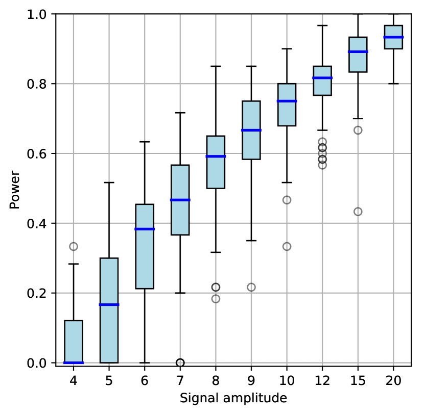
(a)

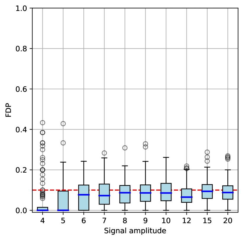
(b)

Figure 5: Power (a) and FDP (b) of our procedure in a simulation with $n=1000$ and $p=1000$, over 100 independent experiments. Variables are distributed as a discrete Markov chain. The knockoff copies are constructed using the true model parameters. The response $Y|X$ is sampled from a logistic regression model. The dashed red line in (b) indicates the target FDR level $\alpha=0.1$.

6.1.3 Robustness to overfitting

In the previous example, we generated the knockoff variables using the real distribution of $X$. However, in most practical applications this is not known exactly and it must be estimated from the available data. In a more realistic situation one may have some prior knowledge that a Markov chain is a good model for the covariates, but ignore the exact form of the transition matrices. Therefore, we repeat the previous experiment, generating instead the knockoff copies $\tilde{X}$ from the fitted values of the Markov chain parameters. The estimates $(\hat{q}_{1},\hat{Q})$ are obtained by maximum-likelihood with Laplace smoothing on all the available observations of $X$. The results shown in Figure 6 and Table 1 are very similar to those of Figure 5. This shows that the FDR is still controlled, and it also suggests that our procedure is robust to fitting the feature distribution.

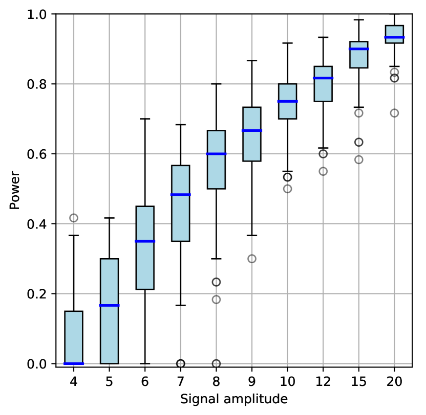
(a)

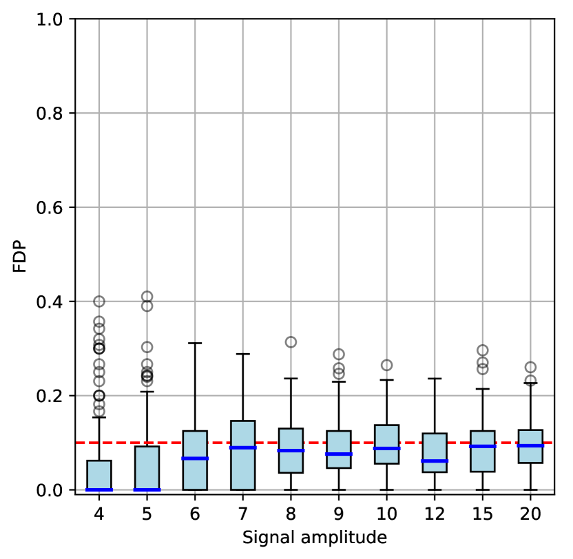
(b)

Figure 6: Power (a) and FDP (b) of our procedure with simulated Markov chain covariates, with knockoffs sampled using estimates of the transition matrices obtained from the same dataset. The setup is otherwise the same as that in Figure 5.

Signal	True $F_{X}$		Estimated $F_{X}$
amplitude	FDR (95% c.i.)	Power (95% c.i.)	FDR (95% c.i.)	Power (95% c.i.)
4	0.050 $\pm\;0.020$	0.051 $\pm\;0.018$	0.054 $\pm\;0.020$	0.064 $\pm\;0.020$
5	0.057 $\pm\;0.017$	0.154 $\pm\;0.031$	0.062 $\pm\;0.019$	0.155 $\pm\;0.031$
6	0.083 $\pm\;0.014$	0.329 $\pm\;0.034$	0.078 $\pm\;0.015$	0.312 $\pm\;0.035$
7	0.084 $\pm\;0.014$	0.446 $\pm\;0.031$	0.091 $\pm\;0.015$	0.449 $\pm\;0.031$
8	0.086 $\pm\;0.012$	0.566 $\pm\;0.025$	0.089 $\pm\;0.013$	0.560 $\pm\;0.029$
9	0.092 $\pm\;0.013$	0.658 $\pm\;0.024$	0.088 $\pm\;0.013$	0.653 $\pm\;0.023$
10	0.093 $\pm\;0.011$	0.730 $\pm\;0.020$	0.096 $\pm\;0.011$	0.741 $\pm\;0.017$
15	0.096 $\pm\;0.011$	0.874 $\pm\;0.016$	0.092 $\pm\;0.012$	0.878 $\pm\;0.014$
20	0.094 $\pm\;0.011$	0.930 $\pm\;0.009$	0.098 $\pm\;0.011$	0.933 $\pm\;0.009$

Table 1: FDR and average power in the numerical experiments of Figure 5 and 6. We compare the results obtained with knockoff variables created using the exact (left) and estimated (right) Markov chain model parameters.

Alternatively, if additional unsupervised samples are available, one can use them to improve the estimation of the covariate distribution. We illustrate this idea by generating unlabeled datasets of varying size $n_{\text{u}}$, from the same population. In principle, one could use both the supervised and the unsupervised observations of $X$ to estimate the parameters of $F_{X}$. However, we choose to fit the parameters only on the latter, in order to better observe the effect of overfitting. For a range of values of $n_{\text{u}}$, we compute $(\hat{q}_{1},\hat{Q})$ and proceed as in the previous examples, repeating the experiment 100 times. The results are shown in Figure 7. We observe that our procedure is robust to overfitting. Even in the extreme cases in which $n_{u}$ is very small (i.e. $n_{u}\leq 50$), the empirical FDR is below the nominal value, while for larger values of $n_{u}$ the validity of the FDR control is clear.

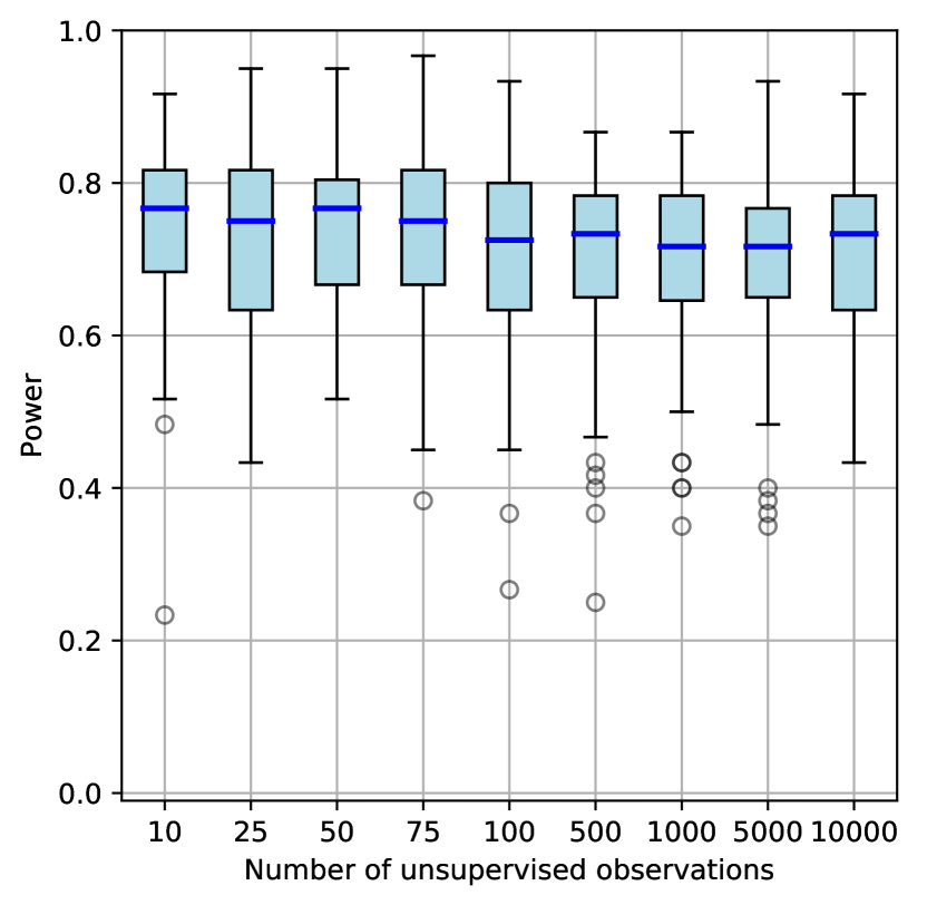
(a)

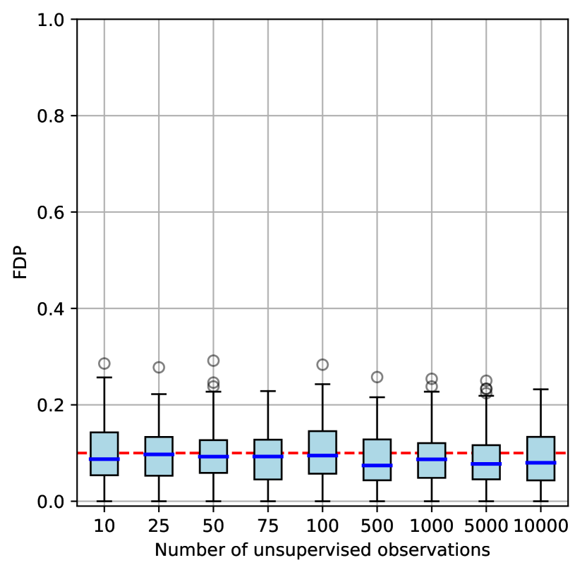
(b)

Figure 7: Power (a) and FDP (b) of our procedure with simulated Markov chain covariates. Knockoffs are sampled using estimates of the transition matrices obtained from an independent dataset of $n_{u}$ unsupervised observations of $X$, for different values of $n_{u}$. The signal amplitude is $a=10$. The setup is otherwise the same as that in Figure 5.

6.2 Knockoffs for HMM variables

We continue our numerical experiments by generating knockoff copies of an HMM.

6.2.1 A toy model

We consider a vector $X$ of $p=1000$ covariates distributed as the HMM defined below. The parametrization that we adopt is loosely inspired by the left-right models used for speech recognition [10], but we do not aim to realistically simulate any specific application. Instead, we prefer to keep the model extremely simple for the sake of exposition. Here, the latent Markov chain $Z\sim\text{MC}(q_{1},Q)$ takes on values in $\{0,1,\ldots,K-1\}^{p}$ and its states evolve “clockwise” according to

$$q_{1}(k)=\begin{cases}1,&k=1,\\ 0,&\text{otherwise},\end{cases} Q_{j}(k|l)=\begin{cases}0.9,&k=l,\\ 0.1,&k=l+1\mod K,\\ 0,&\text{otherwise},\end{cases} j\in\{2,\ldots,p\},$$

for $k,l\in\{0,1,\ldots,K-1\}$. Concretely, we let $K=9$ and we assume for simplicity that all observed variables $X_{j}$ take on values in a set $\mathcal{X}=\{-4,-3,\ldots,+3,+4\}$, also of size $K$. The emission probabilities $f_{j}(x|z)$ are defined, for some $\gamma\in(0,1)$, as

$$f_{j}(x|z) =\begin{cases}\frac{\gamma}{2},&(x+4)=z\text{ or }(x+4)=z+1,\\ \frac{\gamma}{2},&(x+4)=0\text{ and }z=K-1,\\ \frac{1-\gamma}{K-2},&\text{otherwise}.\end{cases}$$

In this example, we set $\gamma=0.35$ because we have observed empirically that it yields an interesting structure with moderately strong correlations.

Conditional on $X=(X_{1},\ldots,X_{p})$, the response $Y$ is sampled from the same binomial generalized linear model of Section 6.1. Again, we vary the signal amplitude in the simulations.

6.2.2 Effect of signal amplitude

We simulate $n=1000$ independent observations of $(X,Y)$ from the model described above. For different values of the signal amplitude $a$, we apply our method to construct knockoff copies of the HMM, using the exact model parameters. We select relevant variables after computing the same importance measures as in Section 6.1, and applying the filter with a knockoff+ threshold (target $\alpha=0.1$). The power and FDP shown in Figure 8 and Table 2 correspond to 100 independent replications of this experiment. The results confirms that our procedure accurately controls the FDR for all values of the signal amplitude.

(a)

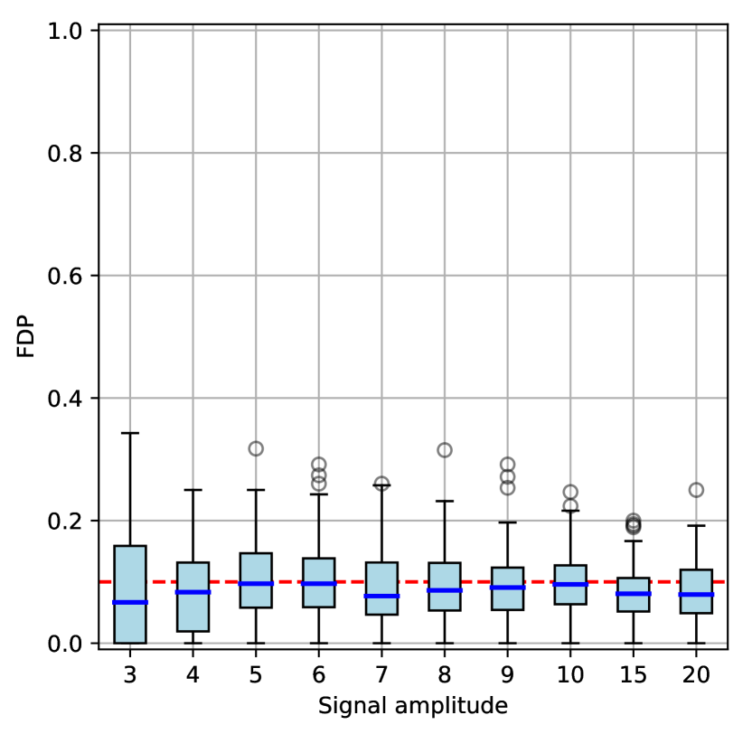
(b)

Figure 8: Power (a) and FDP (b) of our procedure in a simulation with $n=1000$ and $p=1000$, over 100 independent experiments. Variables are distributed as a discrete hidden Markov model. The knockoff copies are constructed using the true model parameters. The response $Y|X$ is sampled from a logistic regression model. The dashed red line in (b) indicates the target FDR level $\alpha=0.1$.

6.2.3 Robustness to overfitting

In the previous example, we have sampled the knockoff variables by exploiting our knowledge of the true distribution of $X$. Now, we continue as in Section 6.1 to verify the robustness of our procedure to the estimation of $F_{X}$. Instead of using the exact values of $(q_{1},Q,f)$, we fit them on the available data using the Baum-Welch algorithm [48]. The power and FDR shown in Figure 9 and Table 2 are estimated over 100 replications, for different values of the signal amplitude. Similarly to the earlier example with Markov chain covariates, our technique behaves robustly and maintains control as expected.

Signal	True $F_{X}$		Estimated $F_{X}$
amplitude	FDR (95% c.i.)	Power (95% c.i.)	FDR (95% c.i.)	Power (95% c.i.)
2	0.037 $\pm\;0.019$	0.030 $\pm\;0.014$	0.049 $\pm\;0.025$	0.029 $\pm\;0.013$
3	0.091 $\pm\;0.019$	0.196 $\pm\;0.028$	0.078 $\pm\;0.019$	0.189 $\pm\;0.033$
4	0.082 $\pm\;0.013$	0.414 $\pm\;0.030$	0.094 $\pm\;0.014$	0.432 $\pm\;0.040$
5	0.102 $\pm\;0.013$	0.610 $\pm\;0.023$	0.094 $\pm\;0.013$	0.592 $\pm\;0.026$
6	0.105 $\pm\;0.012$	0.726 $\pm\;0.020$	0.093 $\pm\;0.011$	0.708 $\pm\;0.022$
7	0.090 $\pm\;0.012$	0.781 $\pm\;0.017$	0.093 $\pm\;0.011$	0.790 $\pm\;0.018$
8	0.093 $\pm\;0.012$	0.830 $\pm\;0.015$	0.086 $\pm\;0.011$	0.839 $\pm\;0.020$
9	0.093 $\pm\;0.011$	0.865 $\pm\;0.013$	0.099 $\pm\;0.010$	0.877 $\pm\;0.012$
10	0.097 $\pm\;0.009$	0.896 $\pm\;0.011$	0.099 $\pm\;0.011$	0.898 $\pm\;0.012$
15	0.083 $\pm\;0.009$	0.945 $\pm\;0.007$	0.093 $\pm\;0.010$	0.950 $\pm\;0.007$
20	0.086 $\pm\;0.009$	0.965 $\pm\;0.006$	0.092 $\pm\;0.010$	0.954 $\pm\;0.007$

Table 2: FDR and average power in the numerical experiments of Figure 8 and 9. We compare the results obtained with knockoff variables created using the exact (left) and estimated (right) hidden Markov model parameters.

Finally, we repeat the experiment by fitting the HMM parameters on an independent and unsupervised dataset of size $n_{\text{u}}$, for different values of $n_{u}$. The results are shown in Figure 10 and they correspond to a range of values for $n_{u}$ and fixed signal amplitude $a=6$. Again, the FDR is consistently controlled. It should not be suprising that this works even when $n_{u}$ is as small as 10. Unlike the numerical experiments with the Markov chain variables considered earlier, the transition matrices and emission probabilities for this HMM are homogeneous for all covariates (i.e. $Q_{j}=Q_{j+1}$, $\forall j$). This simple model results in fewer parameters to be estimated, thus contributing to the overall robustness.

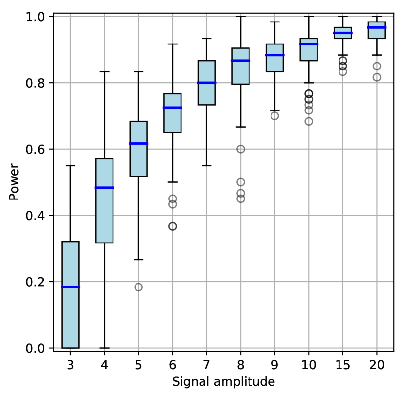
(a)

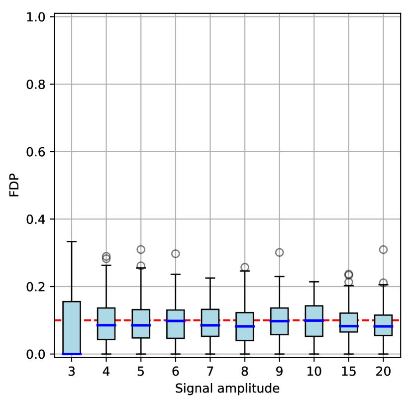
(b)

Figure 9: Power (a) and FDP (b) of our procedure with simulated HMM covariates, with knockoffs sampled using the HMM parameters fitted by EM on the same dataset. The setup is otherwise the same as that in Figure 8.

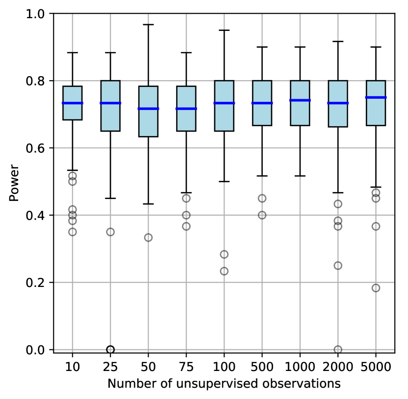
(a)

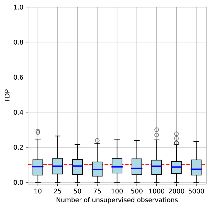
(b)

Figure 10: Power (a) and FDP (b) of our procedure with simulated HMM covariates. Knockoffs are sampled using parameter estimates obtained with EM from an independent dataset of $n_{u}$ unlabeled observations of $X$, for different values of $n_{u}$. The signal amplitude is $a=6$. The setup is otherwise the same as in Figure 8.

6.3 Numerical simulation with real genetic covariates

The results in Section 6.2 suggest that our procedure is robust when the HMM parameters of the covariate distribution are estimated from the available data. However, in those cases the true underlying distribution was indeed decided by us to be an HMM. In this section, we verify that the same robustness holds when the covariates consist of real SNPs data collected in the context of a GWAS.

We consider 29,258 SNPs on chromosome one, genotyped in 14,708 individuals by the Wellcome Trust Case Control Consortium [49]. This is the same set of covariates analyzed in Section 6.1 of [8] and we apply the pre-processing steps described there. We simulate the response according to a conditional logistic regression model of $Y|X$ with $60$ randomly chosen non-zero coefficients. Before proceeding to the data analysis with the knockoff framework, we need to prune the SNPs to make sure that there are no pairs of extremely highly correlated variables among the regressors. This is needed in order for any model selection method to carry out meaningful distinctions between variables. We use the approach described in [8], where a representative is chosen for any cluster of highly correlated SNPs, by selecting the variant among these that is most strongly associated to the phenotype in a hold-out set of 1000 observations (see Section 7.1 for details). This leaves us with a total of 5260 variants. Then, we split the rows of $X$ into 10 folds and separately fit the HMM of Section 5.1 with fastPHASE, using the default configuration and assuming the presence of $K=12$ latent haplotype clusters. Once the parameter estimates are obtained, we construct our knockoff variables according to Algorithm 3. With our software implementation, this last step takes approximatively $0.1$ seconds on a single core of an Intel Xeon CPU (2.60GHz) for each individual. We run the knockoffs procedure on each fold by computing the same feature importance measures $W_{j}=|\hat{\beta}_{j}(\lambda^{\text{CV}})|-|\hat{\beta}_{j+p}(\lambda^{\text{CV}})|$ as in Section 6.1, based on regularized logistic regression with $\ell_{1}$-norm penalty tuned by cross-validation. The selection threshold is chosen as to enforce strict FDR control at level $\alpha=0.1$.

The power and FDP are estimated by comparing our selections to the exact coefficients in the logistic model. For this purpose, a discovery is considered true if and only if any of the highly correlated SNPs in the selected cluster has a non-zero coefficient. The entire experiment is repeated 10 times, starting with the choice of the logistic regression model. This yields a total of 100 point estimates for the power and FDR of our procedure in the unconditional model. The empirical distribution of these two quantities is shown in Figure 11 and Table 3, for different values of the signal amplitude. We observe that the FDR is consistently controlled and the FDP is reasonably concentrated.

The results of this experiment suggest that we can safely proceed with the analysis of GWAS data. Our confidence partially derives from the fact that our procedure enjoys the rigorous robustness of model-free knockoffs for any conditional distribution of the phenotype. As far as type-I error control is concerned, it does not seem consequential that in this experiment we have chosen to simulate the response from a generalized linear model. In fact, the FDR is provably controlled for any $F_{Y|X}$, provided that $F_{X}$ is well-specified. Since we have not artificially simulated the covariates, but used instead real genotypes, we can see no reason why our procedure should not similarly control the FDR once applied to GWAS data.

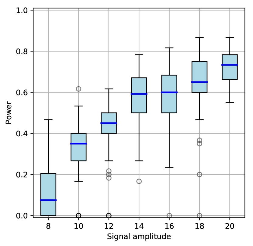
(a)

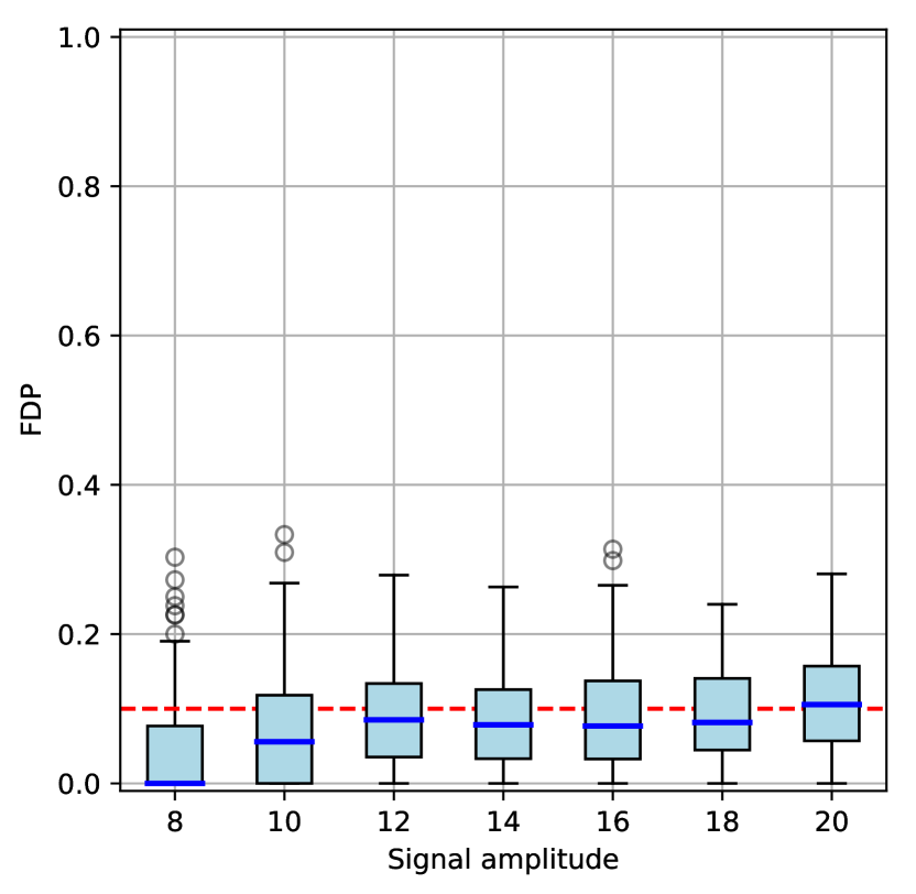
(b)

Figure 11: Power (a) and FDP (b) of our procedure with real genetic variables. One boxplot represents 100 experiments with a total of 10 different logistic regression models for $Y|X$. Apart from the construction of the knockoff variables, this setup is analogous to that of Figure 9 in [8]. The dashed red line in (b) indicates the target FDR level $\alpha=0.1$.

Signal amplitude	FDR (95% c.i.)	Power (95% c.i.)
8	0.040 $\pm\;0.014$	0.121 $\pm\;0.026$
10	0.075 $\pm\;0.015$	0.321 $\pm\;0.026$
12	0.089 $\pm\;0.014$	0.425 $\pm\;0.024$
14	0.086 $\pm\;0.012$	0.571 $\pm\;0.024$
16	0.093 $\pm\;0.015$	0.586 $\pm\;0.028$
18	0.091 $\pm\;0.012$	0.651 $\pm\;0.026$
20	0.112 $\pm\;0.013$	0.718 $\pm\;0.015$

Table 3: FDR and average power in the numerical experiments of Figure 11 with real genetic variables.

7 Applications to GWAS data

We apply our procedure to data from two GWAS: the Northern Finland 1996 Birth Cohort study of metabolic syndrome (NFBC) [50] and the Wellcome Trust Case Control Consortium (WTCCC) [49].

7.1 Analysis of GWAS data

Datasets. NFBC (dbGaP accession number phs000276.v2.p1) comprises observations on 5402 individuals from northern Finland, including genotypes for $\approx 300,000$ SNPs and nine phenotypes. We focus on measurements of cholesterol (HDL and LDL), triglyceride levels (TG) and height (HT), as there is a rich literature on their genetic bases that we can rely upon for comparison. Since not all outcome measurements are available for every subject, the effective values of $n$ are different for each phenotype and a little lower than 5402.

We analyze the control ($n$=2996) and Crohn’s disease (CD) ($n$= 1917) samples from the WTCCC: all of these are typed at $p=377,749$ SNPs.

Data pre-processing. We follow the pre-processing steps of [50] and [33] for the NFBC data. This reduces the total number of SNPs to $p=328,934$. Cholesterol and triglycerides levels are log-transformed prior to analysis, and all response variables are regressed on the top five principal components of the genotype matrix to correct for population stratification [51]. The residuals from these regressions define the phenotypes we actually analyze. The WTCCC data does not require additional pre-processing [49]. A summary of both datasets is shown in Table 4.

SNP pruning. The presence of very high correlations between neighboring SNPs is a well-known issue in genotype association studies and it can be clearly observed in our data. Since many SNPs are very similar to each other, the most compelling scientific question lies in the identification of relevant clusters of tightly linked sites, rather than individual markers. Indeed, the results of the standard GWAS analysis are interpreted as identifying loci (positions in the genome) rather than individual variants—effectively clustering the rejected hypotheses. However, a naïve a-posteriori aggregation of results can inflate the FDR, as the counting of discoveries must be redefined. This issue has been addressed before in special cases [52, 53], but the problem remains that a-posteriori aggregation is intrinsically ill-suited for high-dimensional problems in which the small sample size imposes a limited resolution and makes it fundamentally impossible to distinguish between highly correlated variables. A more natural solution consists of grouping the SNPs a priori, before performing variable selection. By following the steps of [8], we implement an additional pre-processing phase of single-linkage hierarchical clustering, using the empirical correlations as a similarity measure. The SNP clusters are identified by finding the lowest possible cutoff in the dendrogram such that the highest correlation does not exceed 0.5 within any group. Then, we spend a randomly selected subset of the observations (i.e. 20% of the total $n$) to perform marginal t-tests between each variable and the response. The SNP with the smallest p-value in a cluster is chosen as its representative, to be later used with the knockoffs procedure. In both datasets, this process decreases the effective number of variables by a little over $80\%$, as summarized in Table 4.

It must be remarked that the samples used to identify the cluster representatives are not wasted as they can be partially reused without compromising the rigorous FDR-control guarantees. As shown in [33, 8], they can be exploited without violating the exchangeability property (2), provided that the corresponding knockoff copies are created identical to the original variables. Alone, these identical knockoffs would not provide any information to distinguish the relevant variables from the nulls. However, they are useful in improving the accuracy of the importance measures in the knockoff statistics computed for the remaining 80% of the data.

Data source	Response	$n$	$p$ (pre-clustering)	$p$ (post-clustering)
NFBC	HDL (quantitative)	4700	328,934	59,005
NFBC	LDL (quantitative)	4682	328,934	59,005
NFBC	TG (quantitative)	4644	328,934	59,005
NFBC	HT (quantitative)	5302	328,934	59,005
WTCCC	CD (binary)	4913	377,749	71,145

Table 4: Summary of the datasets considered in our analysis. The value of $n$ indicates the number of samples for each response, while the last two columns show the corresponding number of variables before and after clustering. Since clustering was performed on the same empirical correlation matrix for all NFBC traits, the same number of clusters are found. However, the cluster representives may be different because they are selected based on the response.

Knockoff construction. In order to apply Algorithm 3 to construct the knockoff variables, we estimate the HMM parameters $(\hat{r},\hat{\alpha},\hat{\theta})$ of Section 5.1 using fastPHASE. We perform this separately for each of the first 22 chromosomes in the WTCCC and the NFBC data. Since the estimation of the covariate distribution does not make use of the response, we only compute one set of estimates for the NFBC using all of the corresponding SNP sequences. In both cases, we run fastPHASE with a pre-specified number of latent haplotype clusters $K=12$. In its default configuration, the imputation software estimates $\hat{\alpha}$ with the additional constraint that $\alpha_{j,k}$ can only depend on the first index $j$. For simplicity, we do not modify this setting.

Knockoff statistics and filter. We compute the variable importance measures as in Section 6.3, by performing a Lasso regression of $Y$ on the (standardized) knockoff-augmented matrix of covariates $[X,\tilde{X}]\in\{0,1,2\}^{n\times 2p}$, with a regularization parameter $\lambda$ chosen through 10-fold cross-validation. In the case of the Crohn’s disease study, in which the response is binary, the Lasso is replaced by logistic regression with an $\ell_{1}$-norm penalty. Then, relevant SNPs are selected by applying the knockoff filter with the typical knockoff threshold for the target FDR $\alpha=0.1$.

7.2 Results

Selections. We carried the analysis described above on the four datasets of Table 4. Since the model-free knockoffs method is based on a random sample of $\tilde{X}$, in each case our selections depend on its specific realization. Repeating our procedure multiple times and choosing one $\tilde{X}$ after looking at the results would obviously violate the exchangeability conditions required for FDR control. Therefore, we choose instead to report all findings that are selected at least 10 times over 100 independent repeats of the knockoffs procedure. This allows us to provide the reader with both an impression of the variability and an informal measure of confidence for the selections. Our findings are summarized in the Appendix.

Evaluation of findings. Unfortunately, we do not have enough experimental evidence to assess which of our findings are true or false discoveries. However, we can compare our results to those of studies carried out on much larger samples and consider these as the only available approximation of the truth. For lipids we will rely on [54] ($n$=188,577), for height on [55, 56] ($n$= 253,288 and 711,428), and for Crohn’s disease on [57] (22,000 cases and 29,000 controls). Since each of these studies includes a slightly different set of SNPs and our features represent clusters of highly correlated SNPs, some care has to be taken in deciding when the same finding appears in two studies. Each of our SNP clusters spans a genomic locus that can be described by the positions of the first and last SNP. We consider one of our findings to be replicated in the larger study if the latter reported as significant a SNP whose position is within the genomic locus spanned by the cluster of SNPs discovered by our method. Additionally, we highlight clusters that, while not satisfying the definition of “replicated” given above, are less then 0.5 Mb away from a SNP reported in the meta-analyses. These are marked by an asterisk in the supplementary tables contained in the Appendix, to indicate that some independent supporting evidence is available.

Lipids. The results for HDL and LDL cholesterol are shown in Supplementary Table LABEL:table:res_HDL and LABEL:table:res_LDL, respectively. In addition to the results in [54], we compare our findings to those in Sabatti et al. [50], an analysis of our same data based on marginal tests with a level of $5\cdot 10^{-7}$. On average, our method makes 8 discoveries for HDL and 9.8 for LDL. These numbers can be compared to the 5 and 6 discoveries respectively reported in [50]. Among our new findings, some SNPs have been confirmed by the meta-analysis in [54], while others can be found in the works of different authors. However, we prefer to avoid an extensive search over the entire existing literature to avoid selection bias.

We discover on average 2.8 SNPs associated to triglycerides. This is less than the 4 variants identified in [50], but some of our findings are different and one of the additional ones is confirmed by the meta-analysis.

Height. Height is the last trait from the NFBC that we consider. This is known to be a highly polygenic phenotype, with over 700 known variants. However, the effect of each of these variants is very weak and one should not expect to make many discoveries with a dataset as small as ours. We obtain some validation by comparing our findings to the meta-analyses in [55, 56], as shown in Supplementary Table LABEL:table:res_height. Our method discovers 2 relevant SNP clusters, on average. Since this may appear low at first sight, it should be remarked that to the best of our knowledge no other study has found associations for height using only the NFBC data. Of the 4 sites that we select at least 10% of the times, 3 are validated by meta-analysis. The remaining one only appears with frequency equal to 12% and could not be confirmed.

Crohn’s disease. Our findings on the Crohn’s disease data are summarized in Supplementary Table LABEL:table:res_chrons, where we compare them to the meta-analysis in [57] and the original work of the WTCCC [49]. Moreover, we also consider the results of Candes et al. [8]. Their work is the most similar to ours because it uses the same data, pre-processing and clustering method, as well as the overall knockoff methodology. The important distinction is that they construct their knockoff variables differently. Instead of fitting an HMM to the SNP sequences, they assume that the values of the SNPs follow a multivariate normal distribution. Their nominal FDR target $\alpha=0.1$ is the same as ours, and the WTCCC also aims at controlling the Bayesian FDR at approximately the same level. Our method makes 22.8 discoveries on average, versus 18 in [8] and the 9 of the WTCCC. In addition to an apparently higher power in this case, our procedure can in general be expected to enjoy a more principled and safer FDR guarantee. Nowhere have we made the unrealistic assumptions of the WTCCC on the conditional model for the response nor those of [8] on the model for the covariates.

Several of the additional findings that we make have been confirmed in [57], as shown in Supplementary Table LABEL:table:res_chrons. Some of the other selected SNPs may be new discoveries. In this sense, it is encouraging to observe that rs11627513, rs4263839 are reported in the meta-analysis of [59]. The same work also links rs7807268 to the related inflamatory bowel disease, using data from a cohort of 86,682 individuals.

Summary. The results of our data analysis show that our procedure identifies a larger number of potentially significant loci than the traditional methods based on marginal testing (except in the case of triglycerides, for which very few findings are obtained with either approach). In Figure 12, the distribution of the number of discoveries over 100 independent realizations of our knockoff variables is compared to the corresponding fixed quantity from the standard genomic analysis on the same dataset. We can thus verify that, while model-free knockoffs are intrinsically random, we consistently select more variables. We can expect that many of our new findings are valid, but it is impossible to compute the statistical power or the FDR in a GWAS without having access to the ground truth. We find it nonetheless tempting to look at the proportion of our discoveries that is confirmed by the corresponding meta-analyses. Its distribution is shown in Figure 13, separately for each dataset, and without counting those loci that are only partially confirmed (i.e. marked by an asterisk in Appendix B). If we were to try to naïvely estimate the FDR from these plots, we would obtain a value much larger than the target level $\alpha=0.1$. However, such an estimate would be heavily biased and not very meaningful, since none of the meta-analyses is believed to have correctly identified all revelant associations. Instead, some perspective can be gained by comparing our proportion of confirmed discoveries to that obtained with marginal testing on the same data. In the case of HDL cholesterol and triglycerides, we note that our confirmed proportion is appreciably higher, even though one may have intuitively expected a better aggreement between studies relying on the same testing framework.

In general, it should not be surprising that our results are at least partially consistent with those of previous studies. In spite of the fact that our methodology relies on fundamentally different principles, we have selected relevant variables after computing importance measures based on generalized linear regression. The robustness of our type-I error control is completely unaffected by the validity of such model, but a bias towards the discovery of additive linear effects naturally arises. In future studies, one could discover additional associations by easily deploying our procedure with more complex non-linear measures of feature importance.

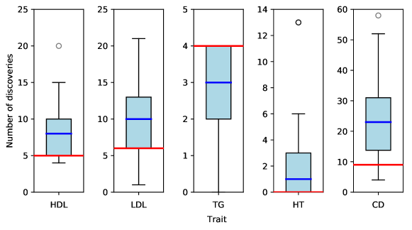
Figure 12: Number of discoveries made on different GWAS datasets. The boxplots refer to our method, for 100 independent realizations of the knockoff variables. The thick red lines indicate the number of discoveries made by the standard genomic analysis of [50] (for HDL, LDL, TG) and [49] (for CD), with the same data.

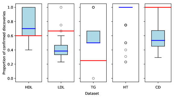
Figure 13: Proportion of the discoveries made with our method that are confirmed by a meta-analysis of [54] (HDL, LDL, TG), [55, 56] (HT) and [57] (CD). The boxplots refer to 100 independent realizations of our knockoff variables. The thick red lines corresponds to the results published in the papers that first analyzed our datasets: [50] (HDL, LDL, TG) and [49] (CD).

8 Discussion

In this paper, we have shown that one can efficiently generate exact knockoff copies of a hidden Markov model. This result extends the applicability of model-free knockoffs beyond the special case of variables following a multivariate normal distribution. Our experiments on real and simulated data provide empirical confirmation of the validity of our entire approach to controlling the selection of relevant variables. At this point, we must note that some important questions still remain unanswered, while we bring about new directions for future research.

• Randomness. Methods based on model-free knockoffs are intrinsically random. Conditionally on the observed $X$ and $Y$, the selection set depends on the specific realization of the knockoff variables $\tilde{X}$. In the applications described earlier, we have observed that different repetitions of our procedure provide reasonably consistent but different answers on the same data. At this point, it is not clear how to best aggregate the different results.

• Group selections. In the presence of extremely high correlatations among the covariates, it is often interesting to ask whether the response depends on a particular group of variables, rather than on each individual one. In our analysis of genetic data, we addressed this point by clustering the variables during the pre-processing phase and restricting the inference to the representatives for each group. Alternatively, one could try to adapt the idea of group-knockoffs in [60] for our method.

• HMM parametrization. We have already mentioned that there exist other forms of HMM that could be adopted for the analysis of genetic data, in addition to that discussed in this paper. Different parametrizations have been developed within the genotype imputation community, and they can be easily exploited by our procedure. For example, if a collection of known haplotypes is available, it is possible to include them in the description of $F_{X}$ used to generate the knockoff copies. It would be interesting to investigate from an applied perspective the relative advantages of one choice over the other.

• Feature importance measures. In the simulations and data analysis of this paper we have computed the knockoff statistics using importance measures based on the cross-validated (logistic) Lasso. Therefore, even though our FDR control does not rely on any assumptions of linearity, the power may be negatively affected if the true likelihood is far from linear. In order to fully exploit the flexibility and robustness of model-free knockoffs, it would be interesting to explore the use of alternative statistics that can better capture interactions and non-linearities (e.g. importance measures based on trees and ensemble methods).

• Beyond HMMs. At this point, we know how to perform controlled variable selection with model-free knockoffs in the special cases where the variables can be described by either an HMM or a multivariate normal distribution. Can this be extended to other classes of covariates? For instance, one may want to consider more general graphical models with a higher-dimensional structure.

In conclusion, we believe that this work offers a significative development within the model-free knockoff framework and it provides a useful statistical contribution to research in genomics. We have argued that our procedure offers a new powerful and natural way of performing variable selection in GWAS, with rigorous finite-sample control of type-I errors relying solely on mild and principled assumptions. Our numerical examples and the data analysis demonstrate its remarkable advantages over marginal testing, which can only be expected to increase as the sample size of the available datasets grows. In fact, with more data at our disposal, we will be able to more accurately estimate the genotype model parameters used to generate the knockoff copies. Moreover, the higher resolution that comes with more observations will allow us to detect important variables that contribute to the response through non-linearities and interactions, as complex and non-parametric measures of variable importance can be easily included in our procedure.

Acknowledgements

E. C. was partially supported by the Office of Naval Research under grant N00014-16-1-2712, and by the Math + X Award from the Simons Foundation. C. S. was partially supported by HG006695 and MH101782 and the Simons Foundation through the Math + X program. We thank Lucas Janson for inspiring discussions and for sharing his computer code.

Appendices

A Model-Free Knockoffs for Discrete Markov Chains

Proof of Proposition 1.

Let us define $Q_{p+1}(k|l)=1$ for all $k,l\in\{1,\ldots,K\}$. We proceed by induction, assuming the induction hypothesis that, for some fixed $j\in\{1,\ldots,p-1\}$, the SCIP algorithm samples all knockoff copies $\tilde{X}_{1:j}$ according to (4). The main step is to show that $\tilde{X}_{j+1}$ is also sampled according to (4). By construction, the SCIP samples $\tilde{X}_{j+1}$ from

$$\mathbb{P}\Big{[} X_{j+1}=\tilde{x}_{j+1}\Big{|}X_{-(j+1)}=x_{-(j+1)},\tilde{X}_{1:j}=\tilde{x}_{1:j}\Big{]}$$

$$\propto\mathbb{P}\left[X_{j+1}=\tilde{x}_{j+1},X_{-(j+1)}=x_{-(j+1)},\tilde{X}_{1:j}=\tilde{x}_{1:j}\right]$$

$$\propto\mathbb{P}\left[X_{j+1}=\tilde{x}_{j+1},X_{-(j+1)}=x_{-(j+1)},\tilde{X}_{1:(j-1)}=\tilde{x}_{1:(j-1)}\right]$$

$$\quad\times\mathbb{P}\left[\left.\tilde{X}_{j}=\tilde{x}_{j}\right|X_{j+1}=\tilde{x}_{j+1},X_{-(j+1)}=x_{-(j+1)},\tilde{X}_{1:(j-1)}=\tilde{x}_{1:(j-1)}\right]$$

$$\propto\mathbb{P}\left[X_{j+1}=\tilde{x}_{j+1},X_{-(j+1)}=x_{-(j+1)}\right]\mathbb{P}\left[\left.\tilde{X}_{1:(j-1)}=\tilde{x}_{1:(j-1)}\right|X_{j+1}=\tilde{x}_{j+1},X_{-(j+1)}=x_{-(j+1)}\right]$$

$$\qquad\times\mathbb{P}\left[\left.\tilde{X}_{j}=\tilde{x}_{j}\right|X_{j+1}=\tilde{x}_{j+1},X_{-(j+1)}=x_{-(j+1)},\tilde{X}_{1:(j-1)}=\tilde{x}_{1:(j-1)}\right].$$

Since we are only interested in the dependence on $\tilde{x}_{j+1}$, the first term above can be simplified as:

$$\mathbb{P}\left[X_{j+1}=\tilde{x}_{j+1},X_{-(j+1)}=x_{-(j+1)}\right] \propto Q_{j+1}(\tilde{x}_{j+1}|x_{j})\,Q_{j+2}(x_{j+2}|\tilde{x}_{j+1}).$$

From the induction hypothesis it follows that the second term is constant with respect to $\tilde{x}_{j+1}$. This is the case because, according to (4), the distribution of $\tilde{X}_{i}$ only depends on $X_{i-1},X_{i+1}$ and $\tilde{X}_{i-1}$, for all $i\leq j$. Therefore, the conditional distribution of all $\tilde{X}_{1:(j-1)}$ only depends on $X_{1:j}$.

At this point, we can focus on the third term:

$$\mathbb{P}\Big{[}\tilde{X}_{j}=\tilde{x}_{j} \Big{|}X_{j+1}=\tilde{x}_{j+1},X_{-(j+1)}=x_{-(j+1)},\tilde{X}_{1:(j-1)}=\tilde{x}_{1:(j-1)}\Big{]}$$

$$=\frac{Q_{j}(\tilde{x}_{j}|x_{j-1})\,Q_{j}(\tilde{x}_{j}|\tilde{x}_{j-1})\,Q_{j+1}(\tilde{x}_{j+1}|\tilde{x}_{j})}{\mathcal{N}_{j-1}(\tilde{x}_{j})\,\mathcal{N}_{j}(\tilde{x}_{j+1})}\propto\frac{Q_{j+1}(\tilde{x}_{j+1}|\tilde{x}_{j})}{\mathcal{N}_{j}(\tilde{x}_{j+1})}.$$

The equality above follows from the fact that the SCIP algorithm samples $\tilde{X}_{j}$ independently of $X_{j}$ as in (4). Thus we can conclude that

$$\mathbb{P}\left[\left.X_{j+1}=\tilde{x}_{j+1}\right|X_{-(j+1)}=x_{-(j+1)},\tilde{X}_{1:j}=\tilde{x}_{1:j}\right] \propto Q_{j+1}(\tilde{x}_{j+1}|x_{j})\,Q_{j+2}(x_{j+2}|\tilde{x}_{j+1})\frac{Q_{j+1}(\tilde{x}_{j+1}|\tilde{x}_{j})}{\mathcal{N}_{j}(\tilde{x}_{j+1})}.$$

This proves that the induction hypothesis also holds for $j+1$. The special case $j=1$ remains to be considered. However, this is straightforward since the SCIP algorithm samples $\tilde{X}_{1}$, independently of $X_{1}$, from

$$\mathbb{P}\left[\left.X_{1}=\tilde{x}_{1}\right|X_{-1}=x_{-1}\right] =\mathbb{P}\left[\left.X_{1}=\tilde{x}_{1}\right|X_{2}=x_{2}\right]\propto\mathbb{P}\left[X_{1}=\tilde{x}_{1},X_{2}=x_{2}\right]=q_{1}(\tilde{x}_{1})Q_{2}(x_{2}|\tilde{x}_{1}).$$

∎

B Results of data analysis

We report below the findings of our data analysis performed on the five phenotypes considered in this paper. An asterisk indicates the presence of a confirmed SNP association within 0.5 Mb of our discovered cluster. We also compute marginal p-values with the standard univariate analysis for all selected SNPs and show the smallest one in each cluster. It must be remarked that our p-values are not identical to those in the original studies, since we have made slightly different methodological choices in the pre-processing and pruning phases, as detailed in Section 7.1. It interesting to look at these p-values because they highlight that many of the marginal signals are weak and could not have been detected by a traditional procedure.

B.1 HDL cholesterol

Table 5: SNP clusters found to be associated with HDL cholesterol over 100 repetitions of our procedure. Positions follow the convention of the Human Genome Build 37, as in the original data. The marginal p-values are obtained from standard univariate linear regression.

Selection frequency	SNP (cluster size)	Chr.	Position range (Mb)	Confirmed in Willer et al. [54]	Found in Sabatti et al. [50]	Marginal p-value
100%	rs1532085 (4)	15	58.68–58.7	rs1532085	rs1532085	$1.33\cdot 10^{-12}$
100%	rs7499892 (1)	16	57.01–57.01	rs3764261	rs3764261	$9.55\cdot 10^{-17}$
100%	rs1800961 (1)	20	43.04–43.04	rs1800961		$2.84\cdot 10^{-8}$
99%	rs1532624 (2)	16	56.99–57.01	rs3764261	rs3764261	$3.08\cdot 10^{-34}$
95%	rs255049 (142)	16	66.41–69.41	rs16942887	rs255049	$1.76\cdot 10^{-08}$
57%	rs10096633 (19)	8	19.73–19.94			$5.33\cdot 10^{-06}$
55%	rs9898058 (1)	17	47.82–47.82			$1.43\cdot 10^{-06}$
51%	rs17075255 (59)	5	164.28–164.92			$1.38\cdot 10^{-05}$
43%	rs3761373 (1)	21	42.87–42.87			$5.96\cdot 10^{-06}$
28%	rs2575875 (10)	9	107.63–107.68	rs3905000		$1.04\cdot 10^{-06}$
23%	rs12139970 (11)	1	230.35–230.42	rs4846914		$1.21\cdot 10^{-05}$
12%	rs173738 (3)	5	16.71–16.73			$4.77\cdot 10^{-06}$

B.2 LDL cholesterol

Table 6: SNP clusters found to be associated with LDL cholesterol. Other details as in caption of Table LABEL:table:res_HDL.

Selection frequency	SNP (cluster size)	Chr.	Position range (Mb)	Confirmed in Willer et al. [54]	Found in Sabatti et al. [50]	Marginal p-value
99%	rs4844614 (34)	1	207.3–207.88		rs4844614	$2.00\cdot 10^{-9}$
97%	rs646776 (5)	1	109.8–109.82	rs629301	rs646776	$2.49\cdot 10^{-9}$
97%	rs2228671 (2)	19	11.2–11.21	rs6511720	rs11668477	$2.28\cdot 10^{-9}$
94%	rs157580 (4)	19	45.4–45.41	rs4420638∗	rs157580	$3.62\cdot 10^{-8}$
92%	rs557435 (21)	1	55.52–55.72	rs2479409		$1.17\cdot 10^{-7}$
80%	rs10198175 (1)	2	21.13–21.13	rs1367117∗	rs693∗	$5.05\cdot 10^{-7}$
76%	rs10953541 (58)	7	106.48–107.3			$3.75\cdot 10^{-6}$
62%	rs6575501 (1)	14	95.64–95.64			$2.32\cdot 10^{-6}$
41%	rs1713222 (45)	2	21.11–21.53	rs1367117	rs693	$4.99\cdot 10^{-11}$
40%	rs2802955 (1)	1	235.02–235.02	rs514230∗		$2.27\cdot 10^{-1}$
37%	rs17129799 (23)	11	96.85–97			$4.84\cdot 10^{-6}$
36%	rs174450 (16)	11	61.55–61.68	rs174546	rs1535	$9.96\cdot 10^{-7}$
26%	rs905502 (1)	8	3.13–3.13			$1.30\cdot 10^{-4}$
25%	rs9696070 (6)	9	89.21–89.24			$1.26\cdot 10^{-5}$
23%	rs166152 (19)	16	29.04–29.33			$4.29\cdot 10^{-5}$
19%	rs12427378 (43)	12	50.43–51.31			$3.69\cdot 10^{-6}$

B.3 Triglycerides

Table 7: SNP clusters found to be associated with triglycerides. Other details as in caption of Table LABEL:table:res_HDL.

Selection frequency	SNP (cluster size)	Chr.	Position range (Mb)	Confirmed in Willer et al. [54]	Found in Sabatti et al. [50]	Marginal p-value
94%	rs10096633 (19)	8	19.73–19.94	rs12678919	rs10096633	$7.47\cdot 10^{-8}$
91%	rs676210 (45)	2	21.11–21.53		rs673548	$2.00\cdot 10^{-7}$
62%	rs2304130 (37)	19	19.28–19.87	rs10401969		$3.91\cdot 10^{-6}$
25%	rs2907632 (13)	17	52.86–52.95			$5.69\cdot 10^{-6}$

B.4 Height

Table 8: SNP clusters found to be associated with height. Other details as in caption of Table LABEL:table:res_HDL.

Selection frequency	SNP (cluster size)	Chr.	Position range (Mb)	Confirmed in Wood et al. [55]	Confirmed in Marouli et al. [56]	Marginal p-value
68%	rs2814982 (120)	6	34.17–35.45	rs12214804	rs2814982	$1.33\cdot 10^{-7}$
46%	rs2882676 (5)	15	89.39–89.4		rs2882676	$2.73\cdot 10^{-6}$
31%	rs6763931 (14)	3	141.04–141.34	rs724016	rs724016∗	$4.00\cdot 10^{-6}$
12%	rs10769671 (17)	11	6.19–6.28			$6.37\cdot 10^{-6}$

B.5 Crohn’s disease

Table 9: SNP clusters found to be associated with Crohn’s disease over 100 repetitions of our procedure. Positions follow the convention of the Human Genome Build 35, as in the original data. The marginal p-values are obtained from the Cochran–Armitage test for trend [61].

Selection frequency	SNP (cluster size)	Chr.	Position range (Mb)	Confirmed in Franke et al. [57]	Found in WTCCC [49]	Found in Candes et. al [8]	Marginal p-value
100%	rs11209026 (2)	1	67.31–67.42	rs11209026	rs11805303	100%	$2.57\cdot 10^{-21}$
99%	rs6431654 (20)	2	233.94–234.11	rs3792109	rs10210302	100%	$1.44\cdot 10^{-14}$
98%	rs6688532 (33)	1	169.4–169.65		rs12037606	90%	$3.48\cdot 10^{-8}$
97%	rs17234657 (1)	5	40.44–40.44	rs11742570	rs17234657	90%	$8.06\cdot 10^{-13}$
95%	rs11805303 (16)	1	67.31–67.46	rs11209026	rs11805303	100%	$5.22\cdot 10^{-14}$
91%	rs7095491 (18)	10	101.26–101.32	rs4409764	rs10883365	100%	$2.81\cdot 10^{-7}$
91%	rs3135503 (16)	16	49.28–49.36	rs2076756	rs17221417	90%	$9.55\cdot 10^{-11}$
81%	rs7768538 (1145)	6	25.19–32.91	rs1799964	rs9469220	60%	$5.83\cdot 10^{-9}$
80%	rs6601764 (1)	10	3.85–3.85		rs6601764	100%	$1.83\cdot 10^{-8}$
75%	rs7655059 (5)	4	89.5–89.53			40%	$2.14\cdot 10^{-7}$
73%	rs6500315 (4)	16	49.03–49.07	rs2076756	rs17221417	60%	$5.73\cdot 10^{-7}$
72%	rs2738758 (5)	20	61.71–61.82	rs4809330		60%	$2.64\cdot 10^{-6}$
70%	rs7726744 (46)	5	40.35–40.71	rs11742570	rs17234657	50%	$7.24\cdot 10^{-13}$
68%	rs11627513 (7)	14	96.61–96.63			80%	$6.70\cdot 10^{-6}$
66%	rs4246045 (46)	5	150.07–150.41	rs7714584	rs1000113	50%	$2.00\cdot 10^{-8}$
62%	rs9783122 (234)	10	106.43–107.61			80%	$1.69\cdot 10^{-4}$
61%	rs6825958 (3)	4	55.73–55.77			30%	$3.54\cdot 10^{-5}$
56%	rs4692386 (1)	4	25.81–25.81			40%	$1.31\cdot 10^{-6}$
56%	rs4263839 (23)	9	114.58–114.78			30%	$3.16\cdot 10^{-5}$
54%	rs2390248 (13)	7	19.8–19.89			50%	$4.53\cdot 10^{-7}$
51%	rs10916631 (14)	1	220.87–221.08			40%	$5.41\cdot 10^{-5}$
49%	rs4437159 (4)	3	84.8–84.81			60%	$5.42\cdot 10^{-5}$
48%	rs9469615 (2)	6	33.91–33.92			30%	$1.13\cdot 10^{-5}$
45%	rs10761659 (53)	10	64.06–64.41	rs10761659	rs10761659	10%	$2.55\cdot 10^{-6}$
42%	rs2836753 (5)	21	39.21–39.23			30%	$1.43\cdot 10^{-6}$
39%	rs6743984 (23)	2	230.91–231.05	rs7423615		10%	$3.79\cdot 10^{-6}$
38%	rs2279980 (20)	5	57.95–58.07			10%	$1.08\cdot 10^{-6}$
35%	rs7186163 (6)	16	49.2–49.25	rs2076756	rs17221417	50%	$7.29\cdot 10^{-8}$
32%	rs16857006 (1)	2	11.1–11.1				$2.30\cdot 10^{-3}$
30%	rs7807268 (5)	7	147.65–147.7			10%	$2.57\cdot 10^{-5}$
27%	rs4807569 (2)	19	1.07–1.08	rs740495			$2.06\cdot 10^{-5}$
24%	rs3779585 (2)	7	90.36–90.38				$7.40\cdot 10^{-6}$
23%	rs12529198 (31)	6	5.01–5.1				$1.08\cdot 10^{-6}$
22%	rs7497036 (19)	15	72.49–72.73				$2.04\cdot 10^{-4}$
20%	rs4959830 (11)	6	3.36–3.41	rs17309827		10%	$9.47\cdot 10^{-7}$
15%	rs13282050 (8)	8	69.3–69.31				$3.64\cdot 10^{-5}$
15%	rs1451890 (26)	15	30.92–31.01				$1.23\cdot 10^{-5}$
14%	rs2814036 (5)	1	163.94–164.07				$9.31\cdot 10^{-7}$
14%	rs7759649 (2)	6	21.57–21.58	rs6908425∗		40%	$1.01\cdot 10^{-4}$
14%	rs4870943 (10)	8	126.59–126.62	rs4871611			$1.46\cdot 10^{-6}$
11%	rs10923347 (1)	1	117.83–117.83				$9.54\cdot 10^{-4}$
10%	rs4438299 (30)	16	60.01–60.32				$7.07\cdot 10^{-5}$

References

- [1] Teri A. Manolio et al. “Finding the missing heritability of complex diseases” In Nature 461.7265 Macmillan Publishers Limited. All rights reserved, 2009, pp. 747–753 DOI: 10.1038/nature08494
- [2] Yoav Benjamini and Yosef Hochberg “Controlling the false discovery rate: a practical and powerful approach to multiple testing” In Journal of the Royal Statistical Society. Series B (Methodological) 57.1 Blackwell Publishing for the Royal Statistical Society, 1995, pp. 289–300 DOI: 10.2307/2346101
- [3] John D. Storey and Robert Tibshirani “Statistical significance for genomewide studies” 12883005[pmid] In Proc Natl Acad Sci USA 100.16 National Academy of Sciences, 2003, pp. 9440–9445 DOI: 10.1073/pnas.1530509100
- [4] Chiara Sabatti, Susan Service and Nelson Freimer “False discovery rate in linkage and association genome screens for complex disorders.” 12807801[pmid] In Genetics 164.2, 2003, pp. 829–833 URL: http://www.ncbi.nlm.nih.gov/pmc/articles/PMC1462572/
- [5] Damian Brzyski et al. “Controlling the rate of GWAS false discoveries” 27784720[pmid] In Genetics 205.1 Genetics Society of America, 2017, pp. 61–75 DOI: 10.1534/genetics.116.193987
- [6] Or Zuk, Eliana Hechter, Shamil R. Sunyaev and Eric S. Lander “The mystery of missing heritability: Genetic interactions create phantom heritability” 22223662[pmid] In Proc Natl Acad Sci U S A 109.4 National Academy of Sciences, 2012, pp. 1193–1198 DOI: 10.1073/pnas.1119675109
- [7] Orjan Carlborg and Chris S. Haley “Epistasis: too often neglected in complex trait studies?” In Nat Rev Genet 5.8 Nature Publishing Group, 2004, pp. 618–625 DOI: 10.1038/nrg1407
- [8] E. Candes, Y. Fan, L. Janson and J. Lv “Panning for gold: model-free knockoffs for high-dimensional controlled variable selection” In ArXiv e-prints, 2016 arXiv:1610.02351 [stat.ME]
- [9] Jeffrey D. Wall and Jonathan K. Pritchard “Haplotype blocks and linkage disequilibrium in the human genome” In Nat Rev Genet 4.8, 2003, pp. 587–597 DOI: 10.1038/nrg1123
- [10] B.. Juang and L.. Rabiner “Hidden Markov models for speech recognition” In Technometrics 33.3 Alexandria, Va, USA: American Society for Quality ControlAmerican Statistical Association, 1991, pp. 251–272 DOI: 10.2307/1268779
- [11] J.. Boreczky and L.. Wilcox “A hidden Markov model framework for video segmentation using audio and image features” In Acoustics, Speech and Signal Processing, 1998. Proceedings of the 1998 IEEE International Conference on 6, 1998, pp. 3741–3744 vol.6 DOI: 10.1109/ICASSP.1998.679697
- [12] Anders Krogh et al. “Hidden Markov models in computational biology” In Journal of Molecular Biology 235.5, 1994, pp. 1501–1531 DOI: http://dx.doi.org/10.1006/jmbi.1994.1104
- [13] Richard Hughey and Anders Krogh “Hidden Markov models for sequence analysis: extension and analysis of the basic method” In Bioinformatics 12.2, 1996, pp. 95 DOI: 10.1093/bioinformatics/12.2.95
- [14] Anders Krogh “Two methods for improving performance of a HMM and their application for gene finding” In Proceedings of the 5th International Conference on Intelligent Systems for Molecular Biology AAAI Press, 1997, pp. 179–186 URL: http://dl.acm.org/citation.cfm?id=645632.663044
- [15] K. Wang et al. “PennCNV: an integrated hidden Markov model designed for high-resolution copy number variation detection in whole-genome SNP genotyping data” In Genome Res. 17.11, 2007, pp. 1665–1674
- [16] Jason Ernst and Manolis Kellis “ChromHMM: automating chromatin-state discovery and characterization” In Nat Meth 9.3 Nature Publishing Group, a division of Macmillan Publishers Limited. All Rights Reserved., 2012, pp. 215–216 DOI: 10.1038/nmeth.1906
- [17] Daniel Falush, Matthew Stephens and Jonathan K. Pritchard “Inference of population structure using multilocus genotype data: linked loci and correlated allele frequencies.” 12930761[pmid] In Genetics 164.4, 2003, pp. 1567–1587 URL: http://www.ncbi.nlm.nih.gov/pmc/articles/PMC1462648/
- [18] H. Tang et al. “Reconstructing genetic ancestry blocks in admixed individuals” In Am. J. Hum. Genet. 79.1, 2006, pp. 1–12
- [19] Heng Li and Richard Durbin “Inference of human population history from individual whole-genome sequences” In Nature 475.7357 Nature Publishing Group, a division of Macmillan Publishers Limited. All Rights Reserved., 2011, pp. 493–496 DOI: 10.1038/nature10231
- [20] N. Patil et al. “Blocks of limited haplotype diversity revealed by high-resolution scanning of human chromosome 21” In Science 294.5547, 2001, pp. 1719–1723
- [21] M. Stephens, N.. Smith and P. Donnelly “A new statistical method for haplotype reconstruction from population data” In Am. J. Hum. Genet. 68.4, 2001, pp. 978–989
- [22] K. Zhang et al. “A dynamic programming algorithm for haplotype block partitioning” In Proc. Natl. Acad. Sci. U.S.A. 99.11, 2002, pp. 7335–7339
- [23] Z.. Qin, T. Niu and J.. Liu “Partition-ligation-expectation-maximization algorithm for haplotype inference with single-nucleotide polymorphisms” In Am. J. Hum. Genet. 71.5, 2002, pp. 1242–1247
- [24] Na Li and Matthew Stephens “Modeling linkage disequilibrium and identifying recombination hotspots using single-nucleotide polymorphism data” In Genetics 165.4 Genetics, 2003, pp. 2213–2233 URL: http://www.genetics.org/content/165/4/2213
- [25] Paul Scheet and Matthew Stephens “A fast and flexible statistical model for large-scale population genotype data: applications to inferring missing genotypes and haplotypic phase” 43035[PII] In Am J Hum Genet 78.4 The American Society of Human Genetics, 2006, pp. 629–644 URL: http://www.ncbi.nlm.nih.gov/pmc/articles/PMC1424677/
- [26] Jonathan Marchini et al. “A new multipoint method for genome-wide association studies by imputation of genotypes” In Nat Genet 39.7 Nature Publishing Group, 2007, pp. 906–913 DOI: 10.1038/ng2088
- [27] Jonathan Marchini and Bryan Howie “Genotype imputation for genome-wide association studies” Review In Nat Rev Genet 11.7 Nature Publishing Group, 2010, pp. 499–511 URL: http://dx.doi.org/10.1038/nrg2796
- [28] Sharon?R? Browning and Brian?L? Browning “Rapid and accurate haplotype phasing and missing-data inference for whole-genome association studies by use of localized haplotype clustering” 17924348[pmid] In Am J Hum Genet 81.5 American Society of Human Genetics, 2007, pp. 1084–1097 URL: http://www.ncbi.nlm.nih.gov/pmc/articles/PMC2265661/
- [29] Sharon R. Browning and Brian L. Browning “Haplotype phasing: existing methods and new developments” In Nat Rev Genet 12.10 Nature Publishing Group, a division of Macmillan Publishers Limited. All Rights Reserved., 2011, pp. 703–714 DOI: 10.1038/nrg3054
- [30] Yongtao Guan and Matthew Stephens “Practical issues in imputation-based association mapping” In PLOS Genetics 4.12 Public Library of Science, 2008, pp. 1–11 DOI: 10.1371/journal.pgen.1000279
- [31] Yun Li et al. “MaCH: using sequence and genotype data to estimate haplotypes and unobserved genotypes” 21058334[pmid] In Genet Epidemiol 34.8, 2010, pp. 816–834 DOI: 10.1002/gepi.20533
- [32] Rina Foygel Barber and Emmanuel J. Candès “Controlling the false discovery rate via knockoffs” In Ann. Statist. 43.5 The Institute of Mathematical Statistics, 2015, pp. 2055–2085 DOI: 10.1214/15-AOS1337
- [33] R. Foygel Barber and E.. Candes “A knockoff filter for high-dimensional selective inference” In ArXiv e-prints, 2016 arXiv:1602.03574 [stat.ME]
- [34] Clive J. Hoggart, John C. Whittaker, Maria De Iorio and David J. Balding “Simultaneous analysis of all SNPs in genome-wide and re-sequencing association studies” In PLOS Genetics 4.7 Public Library of Science, 2008, pp. 1–8 DOI: 10.1371/journal.pgen.1000130
- [35] Tong Tong Wu et al. “Genome-wide association analysis by lasso penalized logistic regression” 19176549[pmid] In Bioinformatics 25.6 Oxford University Press, 2009, pp. 714–721 DOI: 10.1093/bioinformatics/btp041
- [36] Jiahan Li et al. “The Bayesian lasso for genome-wide association studies” 21156729[pmid] In Bioinformatics 27.4 Oxford University Press, 2011, pp. 516–523 DOI: 10.1093/bioinformatics/btq688
- [37] Yongtao Guan and Matthew Stephens “Bayesian variable selection regression for genome-wide association studies and other large-scale problems” In Ann. Appl. Stat. 5.3 The Institute of Mathematical Statistics, 2011, pp. 1780–1815 DOI: 10.1214/11-AOAS455
- [38] David H. Alexander and Kenneth Lange “Stability selection for genome-wide association” In Genetic Epidemiology 35.7 Wiley Subscription Services, Inc., A Wiley Company, 2011, pp. 722–728 DOI: 10.1002/gepi.20623
- [39] Alexandre Bureau et al. “Identifying SNPs predictive of phenotype using random forests” In Genetic Epidemiology 28.2 Wiley Subscription Services, Inc., A Wiley Company, 2005, pp. 171–182 DOI: 10.1002/gepi.20041
- [40] Peng Zhao and Bin Yu “On model selection consistency of Lasso” In J. Mach. Learn. Res. 7 JMLR.org, 2006, pp. 2541–2563 URL: http://dl.acm.org/citation.cfm?id=1248547.1248637
- [41] Emmanuel J. Candès and Yaniv Plan “Near-ideal model selection by minimization” In Ann. Statist. 37.5A The Institute of Mathematical Statistics, 2009, pp. 2145–2177 DOI: 10.1214/08-AOS653
- [42] Sara Geer, Peter Bühlmann, Ya’acov Ritov and Ruben Dezeure “On asymptotically optimal confidence regions and tests for high-dimensional models” In Ann. Statist. 42.3 The Institute of Mathematical Statistics, 2014, pp. 1166–1202 DOI: 10.1214/14-AOS1221
- [43] S. Wager and S. Athey “Estimation and inference of heterogeneous treatment effects using random forests” In ArXiv e-prints, 2015 arXiv:1510.04342 [stat.ME]
- [44] Wenguang Sun and T. Cai “Large-scale multiple testing under dependence” In Journal of the Royal Statistical Society. Series B (Statistical Methodology) 71.2 [Royal Statistical Society, Wiley], 2009, pp. 393–424 URL: http://www.jstor.org/stable/40247580
- [45] Zhi Wei, Wenguang Sun, Kai Wang and Hakon Hakonarson “Multiple testing in genome-wide association studies via hidden Markov models” In Bioinformatics 25.21, 2009, pp. 2802 DOI: 10.1093/bioinformatics/btp476
- [46] J Zhu, J S Liu and C E Lawrence “Bayesian adaptive sequence alignment algorithms.” In Bioinformatics 14.1, 1998, pp. 25 DOI: 10.1093/bioinformatics/14.1.25
- [47] Simon L. Cawley and Lior Pachter “HMM sampling and applications to gene finding and alternative splicing” In Bioinformatics 19.suppl 2, 2003, pp. ii36–ii41 DOI: 10.1093/bioinformatics/btg1057
- [48] L.. Rabiner “A tutorial on hidden Markov models and selected applications in speech recognition” In Proceedings of the IEEE 77.2, 1989, pp. 257–286 DOI: 10.1109/5.18626
- [49] WTCCC “Genome-wide association study of 14,000 cases of seven common diseases and 3,000 shared controls” In Nature 447.7145, 2007, pp. 661–678 DOI: 10.1038/nature05911
- [50] Chiara Sabatti et al. “Genome-wide association analysis of metabolic traits in a birth cohort from a founder population” In Nat Genet 41.1 Nature Publishing Group, 2009, pp. 35–46 DOI: 10.1038/ng.271
- [51] Alkes L. Price et al. “Principal components analysis corrects for stratification in genome-wide association studies” In Nat Genet 38.8, 2006, pp. 904–909 DOI: 10.1038/ng1847
- [52] M. Pacifico, C. Genovese, I. Verdinelli and L. Wasserman “False Discovery Control for Random Fields” In Journal of the American Statistical Association 99.468 [American Statistical Association, Taylor & Francis, Ltd.], 2004, pp. 1002–1014 URL: http://www.jstor.org/stable/27590480
- [53] D.. Siegmund, N.. Zhang and B. Yakir “False discovery rate for scanning statistics” In Biometrika 98.4, 2011, pp. 979 DOI: 10.1093/biomet/asr057
- [54] Global Lipids Genetics Consortium “Discovery and refinement of loci associated with lipid levels” Article In Nat Genet 45.11 Nature Publishing Group, a division of Macmillan Publishers Limited. All Rights Reserved., 2013, pp. 1274–1283 URL: http://dx.doi.org/10.1038/ng.2797
- [55] Andrew R. Wood et al. “Defining the role of common variation in the genomic and biological architecture of adult human height” Article In Nat Genet 46.11 Nature Publishing Group, a division of Macmillan Publishers Limited. All Rights Reserved., 2014, pp. 1173–1186 URL: http://dx.doi.org/10.1038/ng.3097
- [56] Eirini Marouli et al. “Rare and low-frequency coding variants alter human adult height” Article In Nature 542.7640 Macmillan Publishers Limited, part of Springer Nature. All rights reserved., 2017, pp. 186–190 URL: http://dx.doi.org/10.1038/nature21039
- [57] Andre Franke et al. “Genome-wide meta-analysis increases to 71 the number of confirmed Crohn’s disease susceptibility loci” In Nat Genet 42.12 Nature Publishing Group, a division of Macmillan Publishers Limited. All Rights Reserved., 2010, pp. 1118–1125 DOI: 10.1038/ng.717
- [58] Ulla Sovio et al. “Genetic determinants of height growth assessed longitudinally from infancy to adulthood in the northern Finland birth cohort 1966” In PLoS Genet 5.3 San Francisco, USA: Public Library of Science, 2009, pp. e1000409 DOI: 10.1371/journal.pgen.1000409
- [59] Jimmy Z. Liu et al. “Association analyses identify 38 susceptibility loci for inflammatory bowel disease and highlight shared genetic risk across populations” Article In Nat Genet 47.9 Nature Publishing Group, a division of Macmillan Publishers Limited. All Rights Reserved., 2015, pp. 979–986 URL: http://dx.doi.org/10.1038/ng.3359
- [60] Ran Dai and Rina Foygel Barber “The knockoff filter for FDR control in group-sparse and multitask regression” In Proceedings of the 33rd International Conference on International Conference on Machine Learning - Volume 48, ICML’16 New York, NY, USA: JMLR.org, 2016, pp. 1851–1859 URL: http://dl.acm.org/citation.cfm?id=3045390.3045586
- [61] P. Armitage “Tests for linear trends in proportions and frequencies” In Biometrics 11.3 [Wiley, International Biometric Society], 1955, pp. 375–386 URL: http://www.jstor.org/stable/3001775