JVLA Observations of IC 342: Probing Star Formation in the Nucleus

Abstract

IC 342 is a nearby, late-type spiral galaxy with a young nuclear star cluster surrounded by several giant molecular clouds. The IC 342 nuclear region is similar to the Milky Way and therefore provides an interesting comparison. We explore star formation in the nucleus using radio recombination line (RRL) and continuum emission at 5, 6.7, 33, and 35$\,{\rm GHz}$ with the JVLA. These radio tracers are largely unaffected by dust and therefore sensitive to all of the thermal emission from the ionized gas produced by early-type stars. We resolve two components in the RRL and continuum emission within the nuclear region that lie east and west of the central star cluster. These components are associated both spatially and kinematically with two giant molecular clouds. We model these regions in two ways: a simple model consisting of uniform gas radiating in spontaneous emission, or as a collection of many compact H ii regions in non-LTE. The multiple H ii region model provides a better fit to the data and predicts many dense ($n_{\rm e}\sim 10^{4}-10^{5}$$\,{\rm cm^{-3}}$), compact ($\lesssim 0.1$$\,{\rm pc}$) H ii regions. For the whole nuclear region as defined by RRL emission, we estimate a hydrogen ionizing rate of $N_{\rm L}\sim$ $2\times 10^{52}$$\,{\rm s}^{-1}$, corresponding to equivalent $\sim 2000$ O6 stars and a star formation rate of $\sim 0.15$$\,M_{\odot}\,{\rm yr}^{-1}$. We detect radio continuum emission west of the southern molecular mini spiral arm, consistent with trailing spiral arms.

1 Introduction

Young massive star clusters are found in starburst galaxies, normal galaxies, galactic nuclei, the central regions of mergers, and in tidal tails (Böker et al., 2004; de Grijs, 2004; Knierman et al., 2004; Larsen, 2004). These star clusters have many names such as super star clusters, super-associations, starbursts, etc. The most massive star clusters in the Galaxy reside in the optically obscured Galactic Center region and are small compared to those found in the local Universe. The nearest prototype for these larger star clusters is 30 Doradus in the Large Magellanic Cloud (Ambartsumian, 1954). The Hubble Space Telescope (HST) has been pivotal in discovering more distant star clusters (Holtzman, et al., 1992; Johnson & Conti, 2000; Whitmore, 2003; Leitherer, 2003; O’Connell, 2004). The most dense and massive young star clusters appear to be young versions of classical globular clusters and are an important mode of star formation and evolution.

Very young star clusters are difficult to observe in the UV, optical, or near IR because of the high extinction from their surrounding natal clouds of gas and dust. Radio continuum measurements, however, are excellent probes of these regions where observations at several frequencies can separate the thermal emission, associated with HII regions, and the non-thermal emission, related to supernova remnants (Turner & Ho, 1983; Kobulnicky & Johnson, 1999; Turner et al., 2000; Johnson & Kobulnicky, 2003; Johnson, et al., 2004). The measured Lyman continuum fluxes provide an estimate of the OB stellar luminosities that are typically consistent with far-infrared luminosities (Turner & Ho, 1994). Radio recombination lines (RRLs) are more difficult to detect but yield important information about the dynamics of the brightest, nearby star clusters (Anantharamaiah et al., 1993; Anantharamaiah & Goss, 1996; Anantharamaiah et al., 2000; Mohan et al., 2002). Young massive star clusters have now been detected in about a dozen nearby galaxies in RRL emission, primarily with interferometers where the high spatial resolution can resolve individual clusters for nearby galaxies (e.g., Rodríguez-Rico et al., 2005); otherwise we are probing the bulk emission over a larger region within the galaxy. Both models and observations show that RRL emission is more intense at higher frequencies primarily due to free-free opacity. For example, the 43 GHz RRL emission towards Arp220 is 50 times more intense than the 8 GHz RRL emission (Rodríguez-Rico et al., 2005).

Because RRLs are weaker than optical tracers their use has been limited to only the brightest star forming regions. Improvements in frequency coverage and sensitivity of the Very Large Array, however, have increased the sensitivity to RRL work by almost an order of magnitude (Kepley et al., 2011). At lower frequencies many RRLs can be observed in parallel and averaged to improve the sensitivity for these weaker RRL transitions, and the wider bandwidths provides sufficient coverage to better detect higher frequency RRLs. Therefore, less massive star clusters can now be detected in RRL emission.

Here we focus on the nearby, face-on, late-type spiral galaxy IC 342 which contains a nuclear star cluster. Observations reveal that many of the properties of the nucleus of IC 342 are similar to the Galactic Center (Meier, 2014). For example, the size and mass of the central molecular zones and ionizing photon rates. Therefore, understanding the nuclear star cluster in IC 342 can shed light on star formation in the Galactic Center, where our position in the disk together with dust obscuration limits our view.

Table 1: JVLA Observational Setup

Parameters	Ka-band	C-band
Proposal Code	11B-078	12A-186
Observing Dates	2011 Nov 27, Dec 8, 31	2012 Mar 17; 2012 Jan 1,2
Configuration	D	C
Phase Calibrators	J0228+6721	J0228+6721
Flux Density Calibrators	0542+498 (3C147)	0137+331 (3C48)
Bandpass Calibrators	J0319+4130	J0319+4130
Time on Source (hr)	5.0	3.5
Sky Frequency (GHz)	34.65681694, 32.91281657	4.99214252, 6.72684455
Continuum BW (MHz)	768.0	1024.0
Line BW (MHz)	128.0	16.0
Line BW ($\,{\rm km\,s^{-1}}$)	1160.0, 1160.0	960.0, 711.0
Channel Width (MHz)	1.21	0.0756
Channel Width ($\,{\rm km\,s^{-1}}$)	10.5, 11.0	4.5, 3.4
Number of Channels	128	256

Note. — IC 342 position: RA(J2000) = 03:46:48.514; Dec(J2000) = 68:05:45.98

2 JVLA Observations and Data Reduction

Here we use the National Radio Astronomy Observatory (NRAO) Jansky Very Large Array (JVLA) to observe the RRL and continuum emission at C-band (5 and 6.75$\,{\rm GHz}$) and Ka-band (32 and 34$\,{\rm GHz}$) toward the nuclear region of IC 342. RRLs provide information about the electron density and temperature along with the number of hydrogen ionizing photons emitted nearby early-type stars (e.g., Shaver, 1975; Balser et al., 1999) These diagnostics therefore are an unobscured tracer of high mass star formation. Typically, to constrain H ii region models at least two RRLs separated in frequency are required (e.g., Anantharamaiah et al., 1993; Balser et al., 2016). Table 1 summarizes the JVLA observations. The JVLA configurations were chosen to provide similar spatial sampling between the two frequency bands. Table 2 lists the observed RRL transitions. There are only two RRLs in the 2$\,{\rm GHz}$ sampled at Ka-band separated by about 1.7$\,{\rm GHz}$. At C-band we observed one set of 5 RRLs near 6.75$\,{\rm GHz}$ and another set of 8 RRLs near 5.0$\,{\rm GHz}$.

Table 2: RRL Transitions

	Rest	Baseband
	Frequency	Frequency
Name	(GHz)	(GHz)
Ka-band
H57$\alpha$	34.5964	34.6568
H58$\alpha$	32.8522	32.9128
C-band
H97$\alpha$	7.0954	6.7268
H98$\alpha$	6.8815	6.7268
H99$\alpha$	6.6761	6.7268
H100$\alpha$	6.4788	6.7268
H101$\alpha$	6.2891	6.7268
H106$\alpha$	5.4443	4.9921
H107$\alpha$	5.2937	4.9921
H108$\alpha$	5.1487	4.9921
H109$\alpha$	5.0089	4.9921
H110$\alpha$	4.8742	4.9921
H111$\alpha$	4.7442	4.9921
H112$\alpha$	4.6188	4.9921
H113$\alpha$	4.4978	4.9921

2.1 Ka-band (33 and 35$\,{\rm GHz}$)

The correlator was configured in Open Shared Risk Observing mode to provide two 1$\,{\rm GHz}$ basebands. Each baseband had eight, 128$\,{\rm MHz}$-wide sub-bands. The H57$\alpha$ and H58$\alpha$ lines were placed in the fourth sub-band of the first and second basebands, respectively. The other 7 sub-bands in each baseband measured the continuum emission. We used the Common Astronomy Software Applications (CASA) package to reduce the JVLA data. Observations at these frequencies requires that the observed amplitudes be corrected for atmospheric opacity and the telescope gain as a function of elevation. We used the seasonal average to determine the opacity for observations between 23 December 2011, 19:12 UT to 12 January 2012, 23:37 UT because the weather station was not working between those dates (G. van Moorsel, private communication, 2012). We took the average of the seasonal and measured opacity as the true opacity for the rest of the observations. The gain response as a function of frequency was corrected with the standard telescope gain curves in CASA 4.0.1.

The data were calibrated using the following procedure. First we created a model image of the bandpass calibrator. The flux density and bandpass calibrator phases and amplitudes were determined per integration time (3 s) and then corrections were made. Estimates of the bandpass were derived using the flux density calibrator and a polynominal bandpass solution. The estimated bandpasses were applied to the data and the flux density and bandpass calibrator phases and amplitudes determined per integration time. The flux density scale for the bandpass calibrator was determined using the flux density calibrator and the Perley-Butler 2010 flux density models (Perley & Butler, 2013). Next, an image of the bandpass calibrator was created and used to derive the final bandpasses. As before, the bandpass and complex gain calibrators have their phases and amplitudes corrected per integration (3 s). The bandpass was then determined on a per-channel basis using the bandpass calibrator. The final bandpasses were applied and the bandpass and complex gain calibrator phases and amplitudes determined on a per-integration time and a per-scan basis. The per-scan phases and amplitudes from the complex gain calibrator were applied to the source data. The flux density of the source data was derived using the model of the bandpass calibrator determined in the first part of the calibration.

After the calibration step, the continuum data for the target were combined to form two final continuum data sets at 33$\,{\rm GHz}$ and 35$\,{\rm GHz}$. These data were phase and amplitude self-calibrated. These solutions were applied to the sub-bands containing the line emission.

2.2 C-band (5 and 6.7$\,{\rm GHz}$)

The correlator was configured in Resident Shared Risk Observing mode. Two 1$\,{\rm GHz}$ wide basebands (each with eight 128$\,{\rm MHz}$ wide sub-bands) were used to measure the continuum at 5.0 and 6.7$\,{\rm GHz}$. Thirteen 16$\,{\rm MHz}$ wide sub-bands were tuned to RRLs in the 1$\,{\rm GHz}$ available for each baseband. The lines observed were H97$\alpha$-H101$\alpha$ at 6.7$\,{\rm GHz}$ and H106$\alpha$-H113$\alpha$ at 5.0$\,{\rm GHz}$. Interference is significant at these frequencies, in particular at 6.75$\,{\rm GHz}$. The data were flagged automatically using the RFLAG algorithm (Appendix E in Greisen (2012)). Channels containing particularly egregious interference were flagged outright for the entire data set.

The calibration for the continuum data followed a similar procedure to that for the Ka-band data (§ 2.1). The phases and amplitudes for the bandpass and flux density calibrator were determined per integration as before. The phases and amplitudes for the complex gain calibrator, however, were determined on a per-scan basis. The line data were calibrated similarly to the continuum data except for one significant difference. We used the continuum data to generate a model for the bandpass calibrator instead of the line data since the wider bandwidths of the continuum data produced a better model of the bandpass. This also reduced the time to generate the calibration since only one iteration over the line data was necessary. The bandpass stability for both the line and continuum data was checked using observations of the bandpass calibrator taken every 1.5 hr during the observing run. A few antennas with time variable bandpasses were flagged. To improve the complex gain solutions, the continuum data sets were phase and amplitude self-calibrated. The solutions from the continuum self-calibration were applied to the line data.

2.3 Imaging

Continuum images were created using multi-frequency synthesis and cleaned using multi-scale clean. We adopted a minimum u-v distance to ensure that all images have the same largest angular scale; this distance corresponds to the largest angular scale sampled by the highest frequency continuum data. We also smoothed the images to a common spatial resolution of $4\hbox to0.0pt{.\hss}{{}^{\prime\prime}}5$, which corresponds to the angular resolution of the lowest frequency line data.

Spectral line cubes were continuum subtracted in the u-v space and then imaged using the same spatial scale as the continuum images. We used a uniform velocity resolution of 20$\,{\rm km\,s^{-1}}$ to maximize the signal-to-noise ratio while still resolving the velocity structure of the lines. For the C-band data, the individual spectral line cubes were averaged together to create two “stacked” spectral line cubes near 5 and 6.7$\,{\rm GHz}$. RRL transitions occur at large principal quantum numbers (n $>50$), and therefore only small variations exist in the peak intensity between adjacent Hn$\alpha$ transitions. Here we do not correct for these differences when stacking RRLs.

3 Results

Our goal was to measure the ionizing flux and star formation rate at the center of IC 342 using RRL and continuum emission at four frequencies: 5$\,{\rm GHz}$ (H106$\alpha$-H113$\alpha$), 6.7$\,{\rm GHz}$ (H97$\alpha$-H101$\alpha$), 34$\,{\rm GHz}$ (H58$\alpha$), and 35$\,{\rm GHz}$ (H57$\alpha$). This provides four independent data points to constrain a variety of models. We chose these frequencies to provide maximum leverage for our models based on the results of previous studies (e.g., Anantharamaiah et al., 2000). We need to average (stack) the RRLs at C-band since these lower frequency RRLs are weaker.

The JVLA continuum images are shown in Figure 1 where we only detect emission in the nuclear region of IC 342. We select three regions for analysis based on inspection of the spectral line cubes (see below). The large blue rectangle shown in Figure 1 contains the “whole region” as defined by the RRL emission. The smaller blue rectangles correspond to different RRL features within the channel maps and are denoted as the “East component” and the “West component”. We sum emission over these spatial regions for further analysis and modeling. Integrated RRL spectra are shown in Figure 2 over the whole region, the East component, and the West component. We detect RRL emission at each of the four frequencies listed above, but have stacked all RRLs within each receiver band to increase the signal-to-noise ratio. The Ka-band RRLs are stacked using the same procedure as for the C-band RRLs (see §2.3). This gives us two RRL data points separated over a wide frequency range for modeling. To our knowledge this is the first detection of RRL emission in IC 342. The RRL profiles are best fit by a single Gaussian with a full-width half-maximum (FWHM) line width $\Delta{V}=70-90$$\,{\rm km\,s^{-1}}$. The East component has a center velocity $V_{\rm bary}\sim 45$$\,{\rm km\,s^{-1}}$, significantly higher than the West component with $V_{\rm bary}\sim 15$$\,{\rm km\,s^{-1}}$. The velocity structure between the East and West components is shown in channel images taken from the Ka-band RRL data cubes (Figure 3). The extent of the RRL emission is restricted to the central regions of the JVLA image (See Figure 4).

Tables 3-4 summarize the radio continuum and RRL results. We list the total continuum flux density (thermal plus non-thermal), integrated over the whole region, the East component, and the West component. We estimate a 10% error in the total continuum flux density. The Gaussian fit parameters to the spectra in Figure 2 are listed in Table 4 together with the RRL flux density integrated over the line profile.

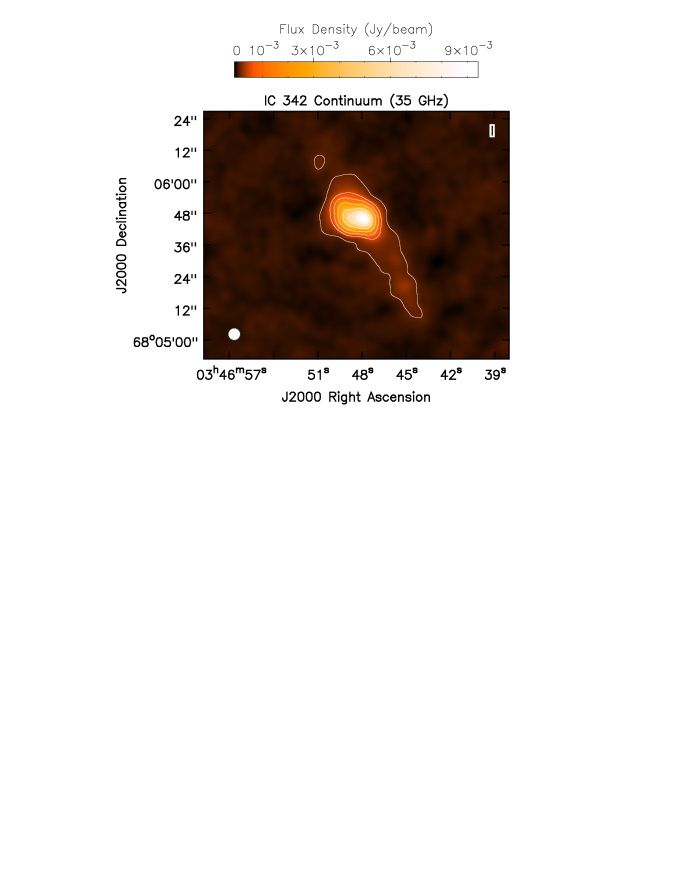
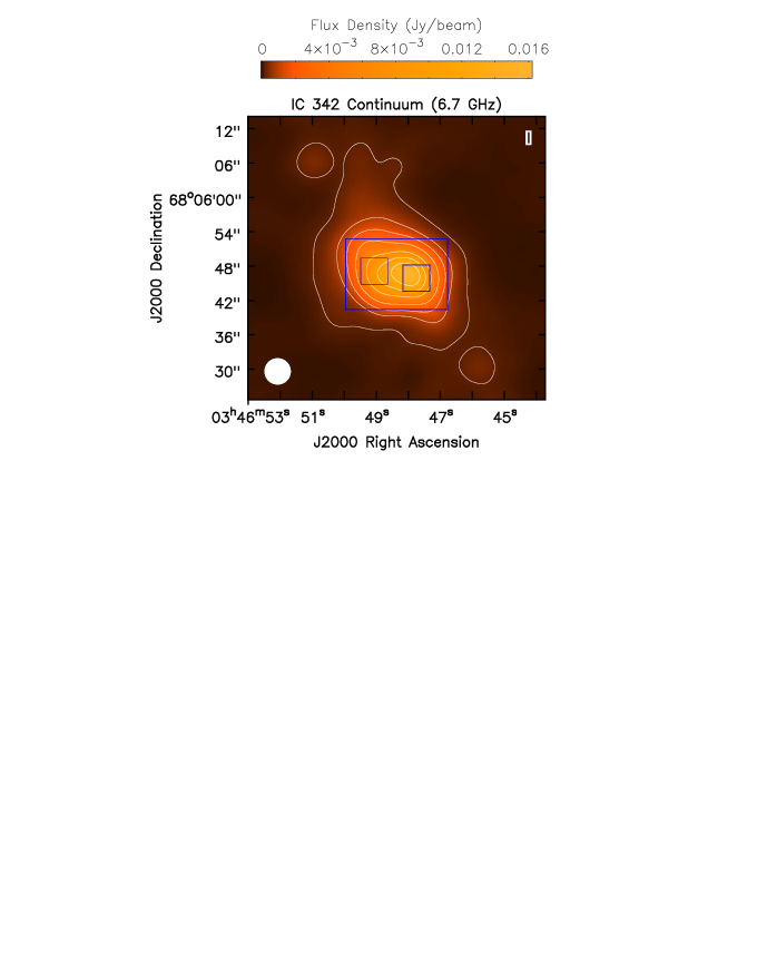
Figure 1: Top: JVLA continuum image of IC 342 at 35$\,{\rm GHz}$. The contour levels are 0.01, 0.05, 0.1, 0.2, 0.4, 0.6, 0.8 times the peak value of 9.45$\rm\,mJy\,beam^{-1}$. The rms noise in the image is 13$\rm\,\mu Jy\,beam^{-1}$. The synthesized beam size, shown in the bottom-left corner, is $4\hbox to0.0pt{.\hss}{{}^{\prime\prime}}5\times 4\hbox to0.0pt{.\hss}{{}^{\prime\prime}}5$. Bottom: JVLA continuum image of IC 342 at 6.7$\,{\rm GHz}$. The contour levels are 0.01, 0.05, 0.1, 0.2, 0.4, 0.6, 0.8 times the peak value of 16.25$\rm\,mJy\,beam^{-1}$. The rms noise in the image is 6.5$\rm\,\mu Jy\,beam^{-1}$. The synthesized beam size, shown in the bottom-left corner, is $4\hbox to0.0pt{.\hss}{{}^{\prime\prime}}5\times 4\hbox to0.0pt{.\hss}{{}^{\prime\prime}}5$. The blue rectangles correspond to the three regions used in the analysis. The “whole region” is the larger box. The “East” and “West” components correspond to the left and right boxes, respectively.

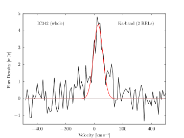
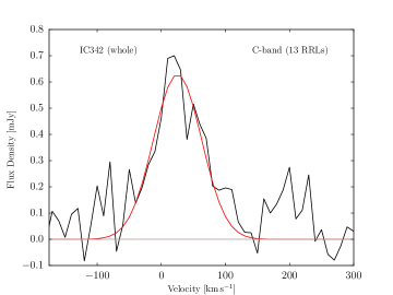
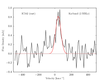
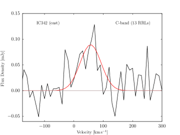
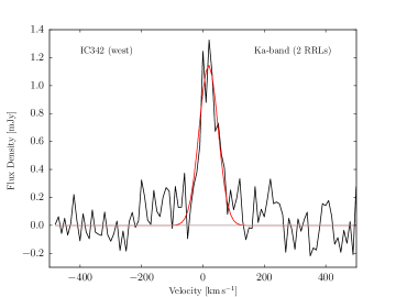
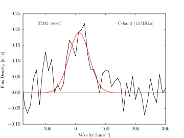
Figure 2: Integrated RRL spectra of the whole region (top), East component (middle), and West component (bottom). The flux density integrated over each region is plotted as a function of the Barycentric velocity. The red curve is a Gaussian fit to the data. Left: Integrated RRL spectrum at Ka-band (H57$\alpha$-H58$\alpha$). Right: Integrated RRL spectrum at C-band (H97$\alpha$-H101$\alpha$ and H106$\alpha$-H113$\alpha$).

Table 3: Radio Continuum Results

	$S^{\rm tot}_{\rm C}$ (mJy)
Freq.	Whole	East	West
(GHz)	Region	Comp.	Comp.
5.0	61.1	10.1	13.5
6.7	51.6	8.4	11.6
34	29.0	4.0	6.9
35	28.6	3.9	6.9

Table 4: Radio Recombination Line Results

		Gaussian Fit
Freq.	$S_{\rm L}^{\rm int}$	$S_{\rm L}^{\rm pk}$	$\Delta V$	$V_{\rm bary}$
(GHz)	(mJy $\,{\rm km\,s^{-1}}$)	(mJy)	($\,{\rm km\,s^{-1}}$)	($\,{\rm km\,s^{-1}}$)
Whole Region
6	$59.1\pm 10.8$	$0.629\pm 0.054$	$88.3\pm 14.3$	$25.3\pm 4.4$
35	$352.1\pm 47.6$	$4.398\pm 0.032$	$75.3\pm 8.5$	$27.4\pm 2.9$
East Component
6	$8.0\pm 3.0$	$0.089\pm 0.014$	$83.9\pm 28.7$	$56.9\pm 11.2$
35	$65.1\pm 14.8$	$0.820\pm 0.102$	$74.5\pm 14.2$	$41.7\pm 4.8$
West Component
6	$16.1\pm 3.2$	$0.192\pm 0.020$	$79.0\pm 13.3$	$12.1\pm 4.9$
35	$88.6\pm 16.6$	$1.145\pm 0.110$	$72.7\pm 11.7$	$18.5\pm 4.3$

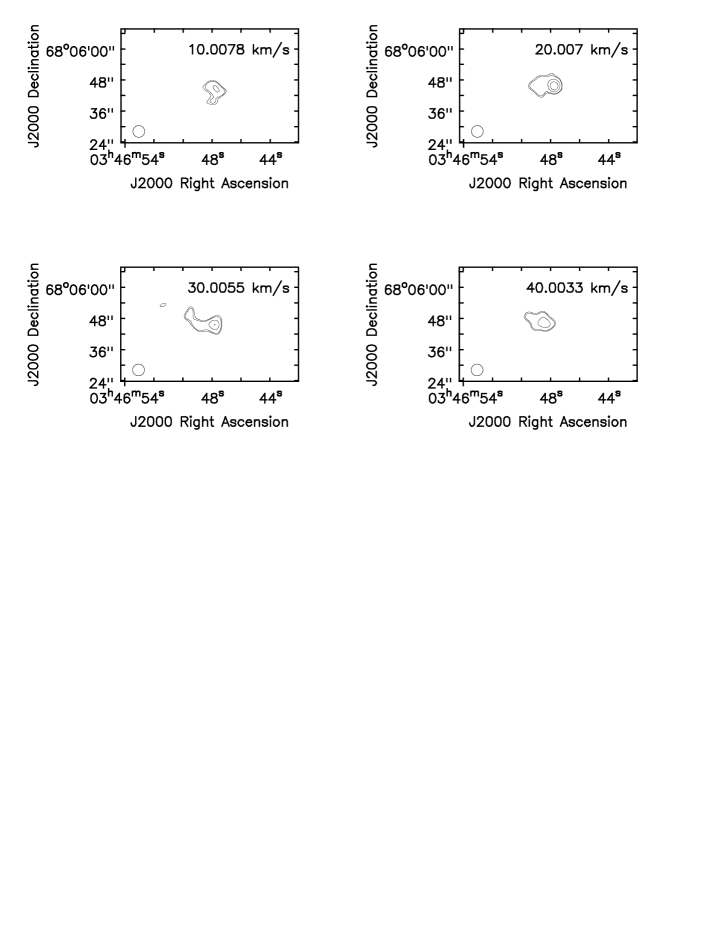
Figure 3: Ka-band RRL channel images. The contours are 0.35, 0.4, 0.6, and 0.8 times the peak emission of 1.74$\rm\,mJy\,beam^{-1}$. The lowest contour level is $3\,\sigma$, where $\sigma\sim 0.2$$\rm\,mJy\,beam^{-1}$ is the rms noise in a single channel image. The Barycentric velocity (optical definition) is shown in the upper right-hand corner of each image. The synthesized beam size ($4\hbox to0.0pt{.\hss}{{}^{\prime\prime}}5\times 4\hbox to0.0pt{.\hss}{{}^{\prime\prime}}5$) is shown in the bottom left-hand corner of each image.

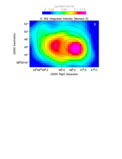
Figure 4: Ka-band RRL integrated intensity map (moment 0). The synthesized beam size, not shown for clarity, is $4\hbox to0.0pt{.\hss}{{}^{\prime\prime}}5\times 4\hbox to0.0pt{.\hss}{{}^{\prime\prime}}5$. The contours are the Ka-band continuum emission shown in Figure 1. The RRL emission is restricted to the nucleus and there is no significant RRL integrated intensity beyond the region shown.

4 H ii Region Models

We fit the JVLA data of the nucleus of IC 342 with two different models, assuming a distance of 3.28$\,{\rm Mpc}$ (Saha et al., 2002). Models based on RRL data typically fall into types: a uniform slab of ionized gas or a collection of compact H ii regions. In many cases the latter model is favored since the uniform slab model often produces an excess of thermal continuum emission (Anantharamaiah et al., 2000).

The first model is very simple and assumes that the nuclear region specified in Figure 1 is fully ionized with gas at a constant electron temperature, $T_{\rm e}$, and electron density, $n_{\rm e}$. H ii regions are primarily heated by the hydrogen-ionizing photons from early-type stars and cooled by collisionally excited lines (e.g., [CII]158$\,\mu{\rm m}$). For OB stars the electron temperature is set primarily by the metallicity (Rubin, 1985) with typical values near $T_{\rm e}=7500$$\,{\rm K}$ in the central regions of the Milky Way (Balser et al., 2011). Following Puxley et al. (1991), we assume that the RRL emission is formed from only spontaneous emission and that the gas is in LTE. That is, there is no stimulated emission. Here we call this the Spontaneous Emission Model (SEM; see §A.1 for details). Given a value of $n_{\rm e}$ allows us to calculate the integrated RRL flux and the thermal continuum flux density. Assuming that the non-thermal continuum flux density follows a power law ($S_{\rm nth}\propto\nu^{\alpha}$), we use the observed total continuum flux density to calculate the spectral index, $\alpha$.

The RRL data fit the model well for low electron densities $n_{\rm e}=25-70$$\,{\rm cm^{-3}}$. For spontaneous, optically thin emission in LTE the integrated line flux is $\propto\nu_{\rm L}^{2}$ (e.g., Puxley et al., 1997), which is consistent with the our results. Using the electron density that best fits the data we derive the corresponding continuum flux density. For each region the predicted continuum flux density is larger than is observed, by as much as a factor of 2.5, and therefore inconsistent with the data. Regardless, we use the RRL results to estimate the star formation rate for this model. In §B, we derive the total number of hydrogen-ionizing photons, $N_{\rm L}$, by balancing the ionization rate versus the recombination rate, assuming a spherical H ii region with diameter equal to the line emitting region size. For the whole region the line emitting size is $L=132$$\,{\rm pc}$. For $n_{\rm e}\sim 25$$\,{\rm cm^{-3}}$ we get $N_{\rm L}=7.2\times 10^{51}\,{\rm s}^{-1}$. This yields a star formation rate of SFR $=0.053$$\,M_{\odot}\,{\rm yr}^{-1}$ (Murphy et al., 2011).

Next, we assume that the nuclear region specified in Figure 1 contains many compact H ii regions that uniformly fill this volume. Following Anantharamaiah et al. (1993), we assume each H ii region is identical with a constant electron temperature, $T_{\rm e}$, electron density, $n_{\rm e}$, and linear size, $\ell$. We call this model the multiple H ii regions model (MHM; see §A.2 for details). The linear size of the line emitting region, $L$, is set by the solid angle of the different regions specified in Figure 1. This model includes non-LTE effects with pressure broadening from electron impacts. There are three free parameters: $T_{\rm e}$, $n_{\rm e}$, and $\ell$. As with the SEM we assume an electron temperature which leaves two data points and two unknowns to constrain the model. We explore the effects of electron temperature on the model by running the grid of ($n_{\rm e}$, $\ell$) for several different fixed $T_{\rm e}$ values. The total number of H ii regions, $N_{\rm HII}$, is set by the ratio of the observed integrated RRL flux to the flux of one H ii region.

The following constraints are used to reject any given model based on physical plausibility (see Anantharamaiah et al., 1993).

1. Filling factor: The H ii regions should be confined to the line emitting region and therefore the filling factor, $f=N_{\rm HII}\,\ell^{3}/L^{3}$, should be less than unity.

2. Peak RRL Intensity: The peak RRL intensity of a single H ii region in the model should be less than the observed peak RRL intensity which covers the entire volume.

3. Minimum Number of H ii Regions: The RRL width from a single H ii region in the model is much less than the observed RRL width due to the velocity motions of the compact H ii regions within the line emitting region. Therefore the number of H ii regions derived from the model, $N_{\rm HII}$, should exceed the minimum number given by $N_{\rm min}=(\Delta{V_{\rm obs}}\Omega_{\rm L})/(\Delta{V_{\rm HII}}\Omega_{\rm B})$, where $\Omega_{\rm B}$ is the beam solid angle.

4. Maximum Number of H ii Regions: The volume of the line emitting region should be able to contain the number of H ii regions constrained by the model. Therefore the total volume of the $N_{\rm HII}$ H ii regions should be smaller than the volume of the line emitting region. Assuming spherical regions this implies that $N_{\rm HII}$ should be less than $N_{\rm max}=(L/\ell)^{3}/N_{\rm HII}$.

5. Thermal Continuum Flux Density: The predicted thermal continuum flux density should be less than the observed (total) flux density.

6. Spectral Index: The measured non-thermal flux density should not be too steep (i.e., $\alpha>-1.5$; see Lisenfeld & Völk (2000)).

A grid of models is run with $n_{\rm e}=100-10^{6}$$\,{\rm cm^{-3}}$ and $\ell=0.01-100$$\,{\rm pc}$. The results are shown in Figure 5 for the whole region. The best fit model is determined by minimizing the root sum square (RSS) between the data and model. Most models fail to pass our constraints. The best models lie along a diagonal line going from larger, diffuse H ii regions to smaller, compact H ii regions. Models above this line fail because the peak line flux for a single H ii region is larger than the observed peak line flux, whereas models below this line fail because the number of H ii regions exceeds the maximum. We use the Ka-band integrated RRL flux to set the number of H ii regions and thus the model goes through this data point. The C-band data may be optically thick and therefore not detect all of the emission.

Table 5 summarizes the results for the whole region, the East component, and the West component. The best models consist of many compact ($\ell\sim 0.05$$\,{\rm pc}$), dense ($n_{\rm e}\sim 5\times 10^{4}$$\,{\rm cm^{-3}}$), H ii regions. The total number of H ii regions is often large ($N_{\rm HII}>1000$), but models with fewer H ii regions (e.g., hundreds) and larger sizes (e.g., $\ell\sim 0.1$) also fit the data well. Regardless, the other properties (e.g., $n_{\rm e}$) are not very sensitive to the H ii region size. The electron temperature does not have a strong effect on the results except for the number of H ii regions and the non-thermal spectral index. We expect the electron temperature to be regulated primarily by the metallicity. Pilyugin et al. (2014) measure 12 + log(O/H) = 8.8 in the central regions of IC 342 which corresponds to $T_{\rm e}=6800$$\,{\rm K}$ (See Shaver et al., 1983). But clearly we do not have sufficient data to constrain $T_{\rm e}$ (see Figure 5). Assuming the continuum emission at 35$\,{\rm GHz}$ is all thermal emission and we are in LTE, the line-to-continuum ratio yields $T_{\rm e}=7150$$\,{\rm K}$ (Balser et al., 2011), consistent with expectations. In all models the non-thermal emission dominates at 6.7$\,{\rm GHz}$, whereas the thermal emission dominates at 35$\,{\rm GHz}$. The continuum data is well fit by assuming the non-thermal emission can be characterized by a power law where for most models $\alpha\sim-0.8$.

Table 5: Multiple H ii Region Model (MHM) Results

	Electron Temperature ($T_{\rm e}$)
Parameter	6000$\,{\rm K}$	7500$\,{\rm K}$	9000$\,{\rm K}$
Whole Region
Electron Density ($n_{\rm e}$) $\,{\rm cm^{-3}}$	$4.6\times 10^{4}$	$4.6\times 10^{4}$	$4.6\times 10^{4}$
H ii Region Size ($\ell$) pc	0.028	0.077	0.077
Number of H ii Region ($N_{\rm HII}$)	66881	3494	4950
Non-thermal Spectral Index ($\alpha$)	$-0.63$	$-0.66$	$-1.03$
H-ionizing rate ($N_{\rm L}$) s-1	$1.9\times 10^{52}$	$1.8\times 10^{52}$	$2.2\times 10^{52}$
Star Formation Rate (SFR) M${}_{\odot}\,$yr-1	0.14	0.13	0.16
East Component
Electron Density ($n_{\rm e}$) $\,{\rm cm^{-3}}$	$4.6\times 10^{4}$	$4.6\times 10^{4}$	$1.3\times 10^{5}$
H ii Region Size ($\ell$) pc	0.077	0.077	0.077
Number of H ii Region ($N_{\rm HII}$)	408	646	57
Non-thermal Spectral Index ($\alpha$)	$-0.75$	$-1.2$	$-0.75$
H-ionizing rate ($N_{\rm L}$) s-1	$2.5\times 10^{51}$	$3.3\times 10^{51}$	$1.9\times 10^{51}$
Star Formation Rate (SFR) M${}_{\odot}\,$yr-1	0.018	0.024	0.014
West Component
Electron Density ($n_{\rm e}$) $\,{\rm cm^{-3}}$	$4.6\times 10^{4}$	$4.6\times 10^{4}$	$4.6\times 10^{4}$
H ii Region Size ($\ell$) pc	0.028	0.028	0.077
Number of H ii Region ($N_{\rm HII}$)	16823	24646	1245
Non-thermal Spectral Index ($\alpha$)	$-0.57$	$-0.95$	$-1.03$
H-ionizing rate ($N_{\rm L}$) s-1	$4.7\times 10^{51}$	$5.8\times 10^{51}$	$5.4\times 10^{51}$
Star Formation Rate (SFR) M${}_{\odot}\,$yr-1	0.034	0.042	0.040

Note. — These models are based on a distance to IC 342 of 3.28$\,{\rm Mpc}$ (Saha et al., 2002).

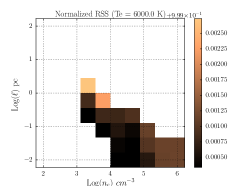
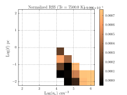
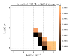
Figure 5: Results for the multiple H ii region model (MHM) for the whole region. From left to right we explore different electron temperatures: $T_{\rm e}=6000$$\,{\rm K}$, 7500$\,{\rm K}$, and 9000$\,{\rm K}$. Top: Normalized root sum squared (RSS) values for the ($n_{\rm e},\ell$) grid of models. The blank areas are models that were not valid (see text). Middle: Integrated RRL flux as a function of frequency. The line corresponds to the best model fit and the points are JVLA data. Bottom: Continuum flux density as a function of frequency. The lines correspond to the thermal, non-thermal and total continuum flux density and the points are JVLA data.

5 Discussion

IC 342 is a face-on, late-type spiral galaxy located in the IC 342/Maffei Group of galaxies at a distance of 3.28$\,{\rm Mpc}$ (Saha et al., 2002). Because the disk is perpendicular to our line-of-sight there is a clear view of the nuclear region which has many similarities to the Galactic Center (Meier, 2014). Both have a central molecular zone, with a similar size and mass, that surrounds a circumnuclear disk. At the center is a star cluster producing a similar number of hydrogen ionizing photons per second. Therefore, the nucleus of IC 342 provides is a nice analog for comparison with the Galactic Center.

IC 342 is near the Galactic equator and thus there is significant obscuration from dust at optical wavelengths, but nevertheless this galaxy is well studied across the electromagnetic spectrum. An HST H$\alpha$ (F656N) image from the Wide Field Planetary Camera 2 (WFPC2) reveals three star clusters within the central 10″ of the nuclear region (see Figure 6). Our JVLA RRL integrated intensity map, overlaid as contours, shows the location and intensity of the thermal emission. The peak RRL emission lies to the east and west of the nuclear star cluster.

Chandra High Resolution Camera (HRC-I) observations of IC 342 resolve X-ray emission in the nucleus into two sources: C12 and C13. The brighter source (C12) lies close to the central star cluster and has an extended component with an X-ray luminosity of $6.7\pm 0.5\times 10^{38}\,$erg s^-1 between $0.08-10\,$kev, consistent with the expectations of a nuclear starburst (Mak et al., 2008). There is some evidence that IC 342 contains a radio-quiet active galactic nuclei based on long term X-ray variability, but this is not conclusive (Mak et al., 2008).

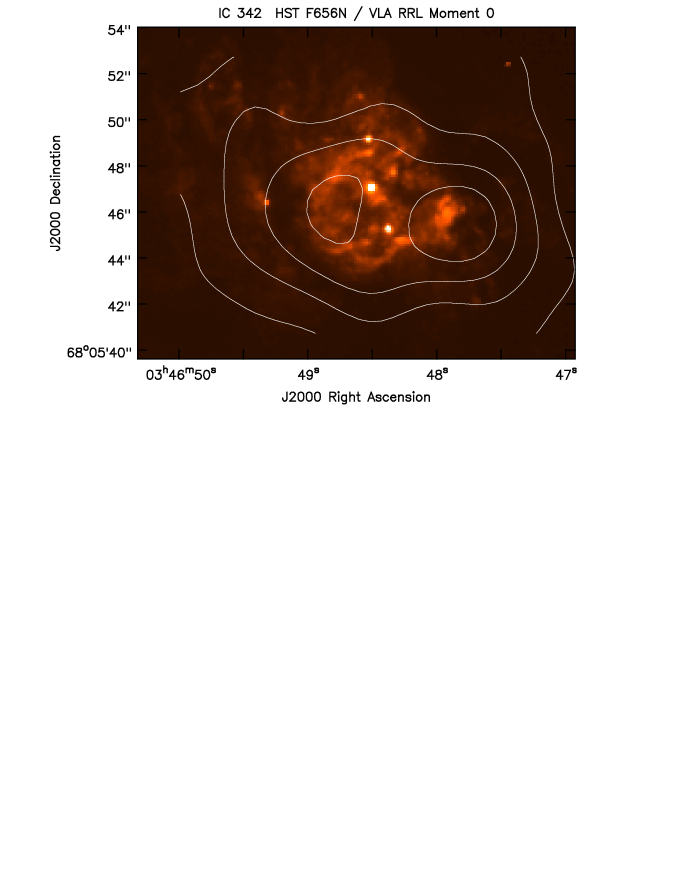
Figure 6: Star formation diagnostics in the IC 342 nuclear region. Shown in color is the HST H$\alpha$ (F656N) image with the JVLA Ka-band RRL integrated intensity map in contours. The contour levels are 0.2, 0.4, 0.6, and 0.8 times the peak intensity ($0.1324\,$Jy beam^-1$\,{\rm km\,s^{-1}}$). The synthesized beam size, not shown for clarity, is $4\hbox to0.0pt{.\hss}{{}^{\prime\prime}}5\times 4\hbox to0.0pt{.\hss}{{}^{\prime\prime}}5$.

In normal galaxies radio continuum observations trace both thermal bremsstrahlung emission from H ii regions and non-thermal synchrotron emission from relativistic electrons in supernova remnants and diffuse gas (Condon, 1992). These processes are typically distinguished by observations at several different frequencies to derive the spectral index ($S_{\rm C}\propto\nu^{\alpha}$), where for thermal emission $\alpha\sim-0.1$ and for non-thermal emission $\alpha\sim-0.5$ to $-1.2$ (Lisenfeld & Völk, 2000). Figure 7 shows the spectral index map created using the C-band (6.7$\,{\rm GHz}$) and Ka-band (35$\,{\rm GHz}$) images. The RRL integrated intensity contour map is overlaid and indicates the location of thermal emission. The spectral index varies between $\alpha\sim-0.2$ (just south of the West RRL component) to $\alpha\sim-0.5$ (in the northwest). This generally agrees with previous work except toward the northeast where we measure $\alpha\sim-0.35$ compared to $\alpha>0$ (c.f. Turner & Ho, 1983; Meier & Turner, 2001). We estimate that the errors in our spectral index map are relatively small over the region shown since the continuum emission is bright.

The radio continuum morphology at 2.6$\,{\rm mm}$ wavelength should primarily trace H ii regions since we expect the non-thermal emission and thermal dust emission to be significantly weaker at these wavelengths. Comparison of the 2.6$\,{\rm mm}$ and 1.3$\,{\rm mm}$ continuum images from Meier & Turner (2001) with our JVLA RRL integrated intensity map are generally in good agreement with two main components surrounding the nuclear star cluster. The RRL East component, however, is located south of the millimeter peak. Meier & Turner (2001) suggest that the 1.3$\,{\rm mm}$ emission is dominated by thermal dust emission based on the spectral index, and that a fraction of the 2.6$\,{\rm mm}$ emission may arise from thermal dust emission. This may explain the differences between their millimeter continuum images and our RRL integrated intensity maps. It is also possible that the gas toward the northeast is optically thick at 35$\,{\rm GHz}$. JVLA continuum observations of IC 342 at cm-wavelengths with higher spatial resolution ($0\hbox to0.0pt{.\hss}{{}^{\prime\prime}}3$) reveal about a dozen compact sources in the nucleus (Tsai et al., 2006). Some of these components are consistent with compact, dense H ii regions as predicted by our models.

We measure a total continuum flux density of 28.6 mJy at 35$\,{\rm GHz}$ over the whole region (see Table 3). We predict a total flux density of $\sim 20$ mJy at 3$\,{\rm mm}$ (see Figure 5), about 25% less than measured by Meier & Turner (2001). Here the “whole region” is defined in terms of the RRL emission. The continuum emission extends beyond the RRL emission (see Figure 1). The continuum emission defined over the full extent of the nucleus is 34 mJy at 35$\,{\rm GHz}$, which accounts for some of this difference. Rabidoux et al. (2014) measured a total flux density of $27.82\pm 1.1$ mJy at 35$\,{\rm GHz}$ using the Green Bank Telescope with a half-power beam-size of 23″. Therefore our JVLA measurements are not missing any significant flux density in the nuclear region due to the lack of zero spacing data. Our models predict a hydrogen-ionizing rate of $N_{\rm L}\sim 2\times 10^{52}\,$s^-1 over the whole region, corresponding to $\sim 2000$ O6 stars of luminosity class V (Martins et al., 2005). Assuming a solar metallicity, continuous star formation, and a Kroupa initial mass function we estimate a SFR $\sim 0.15$$\,M_{\odot}\,{\rm yr}^{-1}$. This is consistent with other estimates based on measurements of the thermal radio continuum emission (Meier & Turner, 2001; Rabidoux et al., 2014).

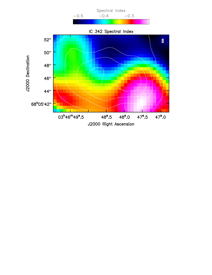
Figure 7: Spectral index map of the nuclear region in IC 342. The spectral index ($S_{\rm C}\propto\nu^{\rm s}$) was calculated using the 6.7$\,{\rm GHz}$ and 35$\,{\rm GHz}$ images. The contours correspond to the Ka-band RRL integrated intensity map with levels as in Figure 6. The synthesized beam size, not shown for clarity, is $4\hbox to0.0pt{.\hss}{{}^{\prime\prime}}5\times 4\hbox to0.0pt{.\hss}{{}^{\prime\prime}}5$.

The molecular gas in the nucleus of IC 342 has been extensively studied with several tracers: CO and various isotopomers (Meier & Turner, 2001; Israel & Baas, 2003); dense gas tracers HCN and HNC (Downes et al., 1992; Meier & Turner, 2005); the kinetic temperature probe NH₃ (Montero-Castaño et al., 2006; Lebrón et al., 2011); and shock tracers SiO and CH₃OH (Meier & Turner, 2005; Usero et al., 2006). The dense molecular gas is concentrated into five giant molecular clouds (GMCs) and forms a mini spiral (Downes et al., 1992). Meier & Turner (2005) observed the nucleus with many molecular tracers at high spatial resolution and proposed the following picture. The mini spiral was created by the response of material from the potential of the bar. As gas collides at the location of the spiral arms energy is lost. This plus tidal torquing allows material to drift inward and trigger star formation where gas piles up at the intersection of the arms and central ring. They suggested trailing spiral arms, where the tips of the arms point toward the direction of gas motion, since the molecular gas densities are higher on the leading (counterclockwise) edges of the spiral arms. Using higher spatial resolution CO and HCN data, Schinnerer et al. (2008) proposed evidence for feedback where star formation alters the flow of molecular material before reaching the nucleus, thereby inhibiting star formation. Röllig et al. (2016) proposed a slightly modified picture where the mini spiral is flipped by 90$\,{}^{\circ}$, creating leading spiral arms. This is based on SOFIA observations of [C ii]$\,158$µm and [N ii]$\,205$µm. The [C ii]$\,158$µm emission arises from the H ii regions and photodissociation regions (PDRs), whereas the [N ii]$\,205$µm emission only traces H ii regions. They detected redshifted emission toward the southeast and blueshifted emission toward the northwest, consistent with leading spiral arms.

The JVLA RRL data probe thermal emission only arising from H ii regions. The RRL East and West components are spatially associated with GMC C and GMC B, respectively, as defined by Downes et al. (1992). The RRL East component is toward the south of GMC C, or near GMC C3 as defined by Meier & Turner (2001). The molecular and ionized thermal gas also have similar velocity structure. The RRL East/GMC C region has velocities between $V_{\rm bary}=40-50$$\,{\rm km\,s^{-1}}$, whereas the RRL west/GMC B region has velocities between $V_{\rm bary}=10-20$$\,{\rm km\,s^{-1}}$. We cannot confirm the velocity structure of the ionized gas observed by Röllig et al. (2016) since the RRL signal falls off quickly from the nuclear region (see Figure 4). We do detect radio continuum emission, however, along the southern spiral arm which is located to the west of the molecular material (see Figure 8). The radio continuum emission is on the leading edge of the arm relative to the molecular material, consistent with the trailing arm picture proposed by Meier & Turner (2005).

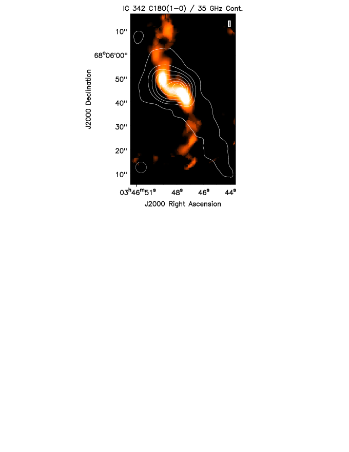
Figure 8: Integrated intensity image of the C¹⁸O(1-0) transition of the central regions of IC 342 from the Owens Valley Millimeter Array (Meier & Turner, 2001). The contours are the JVLA Ka-band continuum emission shown in Figure 1. The circle in the bottom left-hand corner is the beam size of the JVLA data.

6 Summary

IC 342 is a face-on, late-type spiral galaxy with a nuclear region similar to the center of the Milky Way. Here we measure the RRL and continuum emission with the JVLA at C-band (5 and 6.7$\,{\rm GHz}$) and Ka-band (33 and 35$\,{\rm GHz}$), to probe star formation in the nucleus of IC 342. The RRLs consist of H106$\alpha$-H113$\alpha$ at 5$\,{\rm GHz}$; H97$\alpha$-H101$\alpha$ at 6.7$\,{\rm GHz}$; H58$\alpha$ at 34$\,{\rm GHz}$; and H57$\alpha$ at 35$\,{\rm GHz}$. The RRL emission probes thermal emission arising from H ii regions, whereas the continuum emission traces both thermal and non-thermal processes. The RRL data allow us to cleanly separate the thermal and non-thermal emission and also provides kinematic information.

We detect RRL and continuum emission at all frequencies. The RRL emission is concentrated into two components east and west of the nuclear star cluster. These H ii regions concentrations are spatially and kinematically associated with the GMCs measured by dense molecular gas tracers (e.g., HCN). To increase the RRL signal-to-noise ratio we average data over three zones: the “whole region” which encompasses all of the RRL emission; the “East component” which isolates the east RRL component; and the “West component” which isolates the west RRL component.

We model these regions in two ways: a simple model consisting of uniform gas radiating in spontaneous emission (SEM), or as a collection of many compact H ii regions in non-LTE (MHM). The MHM is a better fit to the data and predicts many (hundreds), compact ($\lesssim 0.1$$\,{\rm pc}$), dense ($n_{\rm e}\sim 10^{4}-10^{5}$$\,{\rm cm^{-3}}$) H ii regions. The models cannot constrain the electron temperature or the number of H ii regions very well, but all models predict similar results for the other physical properties. For example, all models that fit the data require compact, dense H ii regions that are consistent with high spatial resolution radio continuum data (e.g., see Tsai et al., 2006). All models predict that the non-thermal emission dominates at 5$\,{\rm GHz}$, whereas the thermal emission dominates at 35$\,{\rm GHz}$. We estimate a non-thermal spectral index $\alpha\sim-0.8$. For the entire nuclear region we calculate a hydrogen ionizing rate of $N_{\rm L}\sim$ $2\times 10^{52}$$\,{\rm s}^{-1}$, consistent with previous estimates based on radio continuum observation alone. This corresponds to a star formation rate of $\sim 0.15$$\,M_{\odot}\,{\rm yr}^{-1}$.

The RRL data provide kinematic information that in principle can constrain the dynamics of the nuclear region. We cannot confirm the proposal by Röllig et al. (2016) that the mini molecular spiral is a leading spiral based on the red/blue-shifted lines of [N ii]$\,205$µm toward the southeast/northwest. The RRLs intensity falls off quickly from the center of the two components. But we do detect radio continuum emission west of the southern molecular mini spiral arm, consistent with trailing spiral arms originally proposed by Meier & Turner (2005).

Appendix A H ii Region Models

Following Puxley et al. (1991), we model the central region of IC 342 in two diverse ways. First we consider a very simple model that assumes the ionized gas has constant density and temperature, and that the RRLs are formed under LTE with no stimulation emission. We call this the spontaneous emission model (SEM). Second, we assume the ionized gas is contained in a collection of compact H ii regions all with the same size, density, and temperature. We call this the multiple H ii region model (MHM). The numerical code was developed in Python and is available on GitHub (Wenger, 2017). Below we describe each model in detail for completeness.

A.1 Spontaneous Emission Model (SEM)

Here we follow Puxley et al. (1991) (also see Bell & Seaquist (1978)) and express the total line flux density from a single H ii region as

$$S_{\rm L}=\Omega_{\rm HII}B(\nu_{\rm L},T_{\rm e})\left[\left(\frac{b_{\rm n}\tau_{\rm L}^{*}+\tau_{\rm c}}{\tau_{\rm L}+\tau_{\rm c}}\right)(1-e^{-(\tau_{\rm L}+\tau_{\rm c})})-(1-e^{-\tau_{\rm c}})\right]+S_{\rm bg}e^{-\tau_{\rm c}}(e^{-\tau_{\rm L}}-1),$$ (A1)

where $\Omega_{\rm HII}$ is the H ii region solid angle, $B(\nu_{\rm L},T_{\rm e})$ is the Planck function, $\nu_{\rm L}$ is the line frequency, $T_{\rm e}$ is the electron temperature, $S_{\rm bg}$ is the background continuum flux density, and $\tau_{\rm c}$ and $\tau_{\rm L}$ are the continuum and line opacity, respectively. The line opacity is $\tau_{\rm L}=b_{\rm n}\beta_{\rm n}\tau_{\rm L}^{*}$, where $b_{\rm n}$ and $\beta_{\rm n}$ are the departure coefficients of the energy level n, and $\tau_{\rm L}^{*}$ is the line opacity in LTE. The contribution from spontaneous emission is then

$$S_{\rm L}=\Omega B(\nu_{\rm L},T_{\rm e})e^{-\tau_{\rm c}}(1-e^{-\tau_{\rm L}})$$ (A2)

where in LTE $\tau_{\rm L}=\tau_{\rm L}^{*}$. The LTE line opacity for Hn$\alpha$ RRLs is approximated by

$$\tau_{\rm L}^{*}=1.7\times 10^{3}\left(\frac{\Delta{\nu}_{\rm L}}{\rm kHz}\right)^{-1}\left(\frac{T_{\rm e}}{\rm K}\right)^{-2.5}\left(\frac{EM}{\rm cm^{-6}\,pc}\right),$$ (A3)

where $EM=\int n_{\rm e}^{2}d\ell$ is the emission measure, $\Delta{\nu}$ is the line width, $n_{\rm e}$ is the electron density, and $d\ell$ is the path length. The thermal continuum flux density is

$$S_{\rm th}=\Omega B(\nu_{\rm L},T_{\rm e})(1-e^{-\tau_{\rm c}}),$$ (A4)

where the continuum opacity is approximated by

$$\tau_{\rm c}=8.2\times 10^{-2}\left(\frac{T_{\rm e}}{\rm K}\right)^{-1.35}\left(\frac{\nu_{\rm L}}{\rm GHz}\right)^{-2.1}\left(\frac{EM}{\rm cm^{-6}\,pc}\right).$$ (A5)

A.2 Multiple H II Regions Model (MHM)

Here we follow Anantharamaiah et al. (1993) where the RRL emission is produced by a collection of $N_{\rm HII}$ identical H ii regions with electron density $n_{\rm e}$, electron temperature $T_{\rm e}$, and linear size $\ell$, embedded in a larger region of continuum emission. From Equation A1 the total flux density emitted from a single H ii region is

$$S_{\rm L}=\frac{2kT_{\rm e}\nu^{2}}{c^{2}}\Omega_{\rm HII}\left[\left(\frac{b_{\rm n}\tau_{\rm L}^{*}+\tau_{\rm c}}{\tau_{\rm L}+\tau_{\rm c}}\right)(1-e^{-(\tau_{\rm L}+\tau_{\rm c})})-(1-e^{-\tau_{\rm c}})\right]+\frac{1}{2}\left(\frac{\Omega_{\rm HII}}{\Omega_{\rm L}}\right)S_{\rm bg}e^{-\tau_{\rm c}}(e^{-\tau_{\rm L}}-1),$$ (A6)

where $\Omega_{\rm L}$ is the solid angle of the entire emitting region. Here we assume the Rayleigh-Jeans limit ($h\nu\ll kT_{\rm e}$) and $B(\nu_{\rm L},T_{\rm e})=2kT_{\rm e}\nu^{2}/c^{2}$. The non-LTE population levels are given by $b_{\rm n}$, whereas $\beta_{\rm n}$ is the amplification term given by

$$\beta_{\rm n}=1-\frac{kT_{\rm e}}{h\nu}\frac{d(\ln\,b_{\rm n})}{d{\rm n}}\Delta{n}.$$ (A7)

We calculate the departure coefficients using the code developed by Salem & Brocklehurst (1979), extended by Walmsley (1990), and available in Appendix E.1 of Gordon & Sorochenko (2009).

For these non-LTE models we use the more accurate expressions for line and continuum optical depth from Viner et al. (1979). The LTE line optical depth is

$$\tau_{\rm L}^{*}=1.4854\times 10^{-22}\,n_{\rm e}n_{\rm i}n^{2}f_{\rm n,m}T_{\rm e}^{-2.5}\,exp\left(\frac{1.57803\times 10^{5}}{n^{2}T_{\rm e}}\right)\frac{H\,\ell}{\Delta{V_{\rm D}}},$$ (A8)

where $n_{\rm e}$ is the electron density in cm^-3, $n_{\rm i}$ is the ion density in cm^-3, $T_{\rm e}$ is the electron temperature in K, $\ell$ is the path length in cm, and $\Delta{V_{\rm D}}$ is the Doppler line width in $\,{\rm km\,s^{-1}}$. For a gas composed of hydrogen and helium

$$n_{\rm i}=n_{\rm e}\left[1+\frac{n_{\rm He^{+}}}{n_{\rm H^{+}}}+\frac{2n_{\rm He^{++}}}{n_{\rm H^{+}}}\right]^{-1}.$$ (A9)

A typical Milky Way value for the singly ionized helium abundance ratio is $n_{\rm He^{+}}/n_{\rm H^{+}}=0.07$ (Wenger et al., 2013). The radiation field that ionized Milky Way H ii regions is not hard enough to produce doubly ionized helium and we therefore set $n_{\rm He^{++}}/n_{\rm H^{+}}=0$. Only in very metal poor H ii regions has doubly ionized helium been detected in significant amounts. Since the metallicity of the central regions of IC 342 is similar to the Solar metallicity we expect little doubly ionized helium to exist. The classical oscillator strength is given by Menzel (1969)

$$f_{\rm n,m}=nM_{1}(\Delta{n})\left[1+\frac{3}{2}\frac{\Delta{n}}{n}+\frac{M_{2}(\Delta{n})}{n^{2}}\right],$$ (A10)

where for $\Delta{n}=1$, $M_{1}=0.1907749$ and $M_{2}=-0.1877268$. We assume the line is broadened by thermal and non-thermal Doppler motions and pressure broadening from electron impacts. The Doppler line width is given by

$$\Delta{V_{\rm D}} = 2(\ln(2))^{1/2}\left(\frac{2kT_{\rm e}}{m_{\rm H}}+\frac{2}{3}\langle V_{\rm T}\rangle^{2}\right)^{1/2}$$ (A11)

$$= 1.66511\left(0.016499\,T_{\rm e}+\frac{2}{3}\langle V_{\rm T}\rangle^{2}\right)^{1/2}{\rm km\,s}^{-1},$$

where $m_{\rm H}$ is the hydrogen mass and the non-thermal Doppler component is expressed in terms of a turbulent velocity, $V_{\rm T}$. Here the units of $T_{\rm e}$ are in K and $V_{\rm T}$ are in $\,{\rm km\,s^{-1}}$. Typical Milky Way H ii region values of the turbulent velocity are $\sim 12$$\,{\rm km\,s^{-1}}$ (Balser et al., 2011). Pressure broadening produces a Lorentzian line shape with wider wings than the Gaussian profile produced by pure Doppler motions. The convolution of a Gaussian and a Lorentzian produces a Voit profile given by

$$H(a,u)=\frac{a}{\pi}\,\int_{-\infty}^{\infty}\frac{exp(-y^{2})dy}{a^{2}+(u-y)^{2}},$$ (A12)

where $a=(\ln\,2)^{1/2}\,\Delta{\nu_{\rm L}}/\Delta{\nu_{\rm D}}$ and $u=2(\ln\,2)^{1/2}(\nu-\nu_{\rm L})/\Delta{\nu_{\rm D}}$. From the Doppler equation $\Delta{\nu_{\rm D}}=\nu\,\Delta{V_{\rm D}}/c$. For hydrogen the Lorentzian-to-Doppler line width ratio is approximated as

$$\frac{\Delta{\nu_{\rm L}}}{\Delta{\nu_{\rm D}}}\approx 9.76\times 10^{-16}\,n_{\rm e}T_{\rm e}^{-1/2}T_{\rm D}^{-1/2}\frac{n^{7}}{\Delta{n}}\left[-11.4+\ln\left(T_{\rm e}\frac{n}{\Delta{n}}\right)\right],$$ (A13)

where the Doppler temperature is $T_{\rm D}=T_{\rm e}+40.42\,\langle V_{\rm T}^{2}\rangle$. Here the electron density has units of cm^-3 and the temperatures are in Kelvin.

The thermal continuum opacity is

$$\tau_{\rm c}=9.7699\times 10^{-21}\,T_{\rm e}^{-1.5}\nu^{-2}n_{\rm e}n_{\rm iT}\,A\,\ell,$$ (A14)

where $T_{\rm e}$ is the electron temperature in K, $\nu$ is the frequency in GHz, $n_{\rm e}$ is the electron density in cm^-3 , and $\ell$ is the path length in cm. Also,

$$n_{\rm iT}=n_{\rm e}\left[1+\frac{n_{\rm He^{+}}}{n_{\rm H^{+}}}+\frac{4n_{\rm He^{++}}}{n_{\rm H^{+}}}\left(1-\frac{\ln\,2}{A}\right)\right]\left[1+\frac{n_{\rm He^{+}}}{n_{\rm H^{+}}}+\frac{2n_{\rm He^{++}}}{n_{\rm H^{+}}}\right]^{-1},$$ (A15)

and $A=\ln(0.04955\,T_{\rm e}^{1.5}/\nu)$.

The number of H ii regions, $N_{\rm HII}$, is calculated by taking the total observed line flux and dividing by the integrated line flux for one region ($S_{\rm int}^{\rm HII}$). Assuming a Gaussian line profile $S_{\rm int}^{\rm HII}=1.064\,S_{\rm L}(\nu=\nu_{\rm L})\,\Delta{V_{\rm D}}$, where the line width is expressed as the FWHM. The thermal continuum flux density is

$$S_{\rm th} = \frac{2k\nu^{2}}{c^{2}}\Omega_{\rm HII}T_{\rm e}(1-e^{-\tau_{\rm c}})N_{\rm HII}\,\,\,\,\,\,\,\tau_{\rm c}\ll 1$$ (A16)

$$= \frac{2k\nu^{2}}{c^{2}}\Omega_{\rm L}T_{\rm e}(1-e^{-\tau_{\rm c}^{\rm los}})\,\,\,\,\,\,\,\,\,\,\,\,\,\,\,\,\,\,\,\,\,\tau_{\rm c}\gtrsim 1$$

where $\tau_{\rm c}^{\rm los}=N_{\rm HII}^{\rm los}\tau_{\rm c}$ and $N_{\rm HII}^{\rm los}=N_{\rm HII}\frac{\ell^{2}}{L^{2}}$. Here $\ell$ is the linear size of an single H ii region, whereas $L$ is the linear size of the line-emitting region. So if the continuum optical depth is small we just multiple the flux density of one H ii region times the number of H ii regions. As the optical depth becomes large we approximate the total flux using the optical depth along the line-of-sight, $\tau_{\rm c}^{\rm los}$. The non-thermal flux density is then

$$S_{\rm nth}=S_{\rm tot}-S_{\rm th}$$ (A17)

where $S_{\rm tot}$ is the observed continuum flux density. But $S_{\rm nth}$ is the result of an intrinsic non-thermal emission, $S_{\rm nth0}$, absorbed by free-free processes from the intervening H ii regions or

$$S_{\rm nth}\approx S_{\rm nth0}\left[1-\frac{1}{2}N_{\rm HII}^{\rm los}\,(1-e^{-\tau_{\rm c}})\right].$$ (A18)

This assumes a random distribution of H ii regions within the line-emitting region, $L$, and thus that on average every H ii region is located half-way inside this region. This approximation is valid for all values of $N_{\rm HII}^{\rm los}$ for $\tau_{\rm c}\ll 1$ and all values of $\tau_{\rm c}$ if $N_{\rm HII}^{\rm los}<1$. Assuming $S_{\rm nth0}\propto\nu^{\alpha}$ we can estimate a non-thermal spectral index.

Appendix B Star Formation Rate

We estimate the star formation rate (SFR) using Starburst99, a software program designed to model various properties of star forming galaxies (Leitherer et al., 1999). Following Murphy et al. (2011), we calculate the SFR by assuming solar metallicity, continuous star formation, and a Kroupa initial mass function for stellar masses between $0.1-100$$\,M_{\odot}$ as

$$SFR=7.29\times 10^{-54}\left(\frac{N_{\rm L}}{\rm s^{-1}}\right)\,\,\,\,\,{\rm M}_{\odot}\,{\rm yr}^{-1},$$ (B1)

where $N_{\rm L}$ is the number of hydrogen-ionizing photons emitted per second (c.f., Calzetti et al., 2007). For an ionization bounded nebula the total number of ionizations equals the number of recombinations. Assuming a spherical geometry

$$N_{\rm L}=\frac{4\,\pi}{3}R^{3}n_{\rm e}^{2}\alpha_{\rm B},$$ (B2)

where $R$ is the radius and $\alpha_{\rm B}$ is the case B recombination rate. Hui & Gnedin (1997) approximate the recombination rate by

$$\alpha_{\rm B}=2.753\times 10^{-14}\frac{\lambda_{\rm HI}^{1.5}}{[1+(\lambda_{\rm HI}/2.740)^{0.407}]^{2.242}}\,\,\,\,\,{\rm cm}^{-3}\,{\rm s}^{-1},$$ (B3)

where $\lambda_{\rm HI}=315614/T_{\rm e}$. This approximation is a fit to the data in Ferland et al. (1992) and is accurate to between 0.7% and 1% for temperatures up to $10^{9}\,$K.

For the SEM we use the line-emitting region size to calculate the radius (i.e., $R=L/2$), whereas for the MHM we use the single H ii regions size (i.e., $R=\ell/2$). For the MHM we multiply $N_{\rm L}$ for a single H ii region by the number of H ii regions, $N_{\rm HII}$, to calculate the total number of hydrogen-ionizing photons emitted per second within the region modeled.

References

- Ambartsumian (1954) Ambartsumian, V.A. 1954, I.A.U. Transactions, 8, 665
- Anantharamaiah & Goss (1996) Anantharamaiah, K. R., & Goss, W. M. 1996, ApJ, 466, L13
- Anantharamaiah et al. (2000) Anantharamaiah, K. R., Viallefond, F., Mohan, N. R., Goss, W. M., & Zhao, J.-H. 2000, ApJ, 537, 613
- Anantharamaiah et al. (1993) Anantharamaiah, K. R., Zhao, J.-H., Goss, W. M., & Viallefond, F. 1993, ApJ, 419, 585
- Babu & Feigelson (2006) Babu, G. J., & Feigelson, E. D. 2006, in ASP Conf. Ser. 351, Astronomical Data Analysis Software and Systems XV, ed. C. Gabriel, C. Arviset, D. Ponz, & S. Enrique (San Francisco, CA: ASP), 127
- Balser et al. (1999) Balser, D. S., Bania, T. M., Rood, R. T., & Wilson, T. L. 1999, ApJ, 510, 759
- Balser et al. (2011) Balser, D. S., Rood, R. T, Bania, T. M., & Anderson, L. D. 2011, ApJ, 738, 27
- Balser et al. (2016) Balser, D. S., Roshi, D. A., Jeyakumar, S., et al. 2016, ApJ, 824, 125
- Bell & Seaquist (1978) Bell, M. B., & Seaquist, E. R. 1978, ApJ, 223, 378
- Böker et al. (2004) Böker, T., Walcher, C.-J., Rix, H.-W., et al. 2004, in ASP Conf. Ser. 322, The Formation and Evolution of Massive Young Star Clusters, ed. H.J.G.L.M. Lamers, L.J. Smith, and A. Nota (San Francisco: ASP), 39
- Calzetti et al. (2007) Calzetti, D., Kennicutt, R. C., Engelbracht, C. W. et al. 2007, ApJ, 666, 870
- Condon (1992) Condon, J. J. 1992, ARA&A, 30, 575
- de Grijs (2004) de Grijs, R. 2004, in ASP Conf. Ser. 322, The Formation and Evolution of Massive Young Star Clusters, ed. H.J.G.L.M. Lamers, L.J. Smith, and A. Nota (San Francisco: ASP), 29
- Downes et al. (1992) Downes, D., Radford, S. J. E., Guilloteau, S., et al. 1992, A&A, 262, 424
- Ferland et al. (1992) Ferland, G. J., Peterson, B. M., Horne, K., Welsh, W. F., & Nahar, S. N. 1992, ApJ, 387, 95
- Gordon & Sorochenko (2009) Gordon, M. A., & Sorochenko, R. L. 2009, Astronomy and Space Science Library, Vol. 282, Radio Recombination Lines
- Greisen (2012) Greisen, E. 2012, AIPS Cookbook
- Holtzman, et al. (1992) Holtzman, C. et al. 1988, A&A, 201, 23
- Hui & Gnedin (1997) Hui, L., & Gnedin, N. Y. 1997, MNRAS, 292, 27
- Israel & Baas (2003) Israel, F. P., & Baas, F. 2003, A&A, 404, 495
- Johnson & Conti (2000) Johnson, K. E., & Conti, P. S. 2000, AJ, 119, 2146
- Johnson, et al. (2004) Johnson, K. E., Indebetouw, R., Watson, C., & Kobulnicky, H. A. 2004, AJ, 128, 610
- Johnson & Kobulnicky (2003) Johnson, K. E. & Kobulnicky, H. A. 2003, ApJ, 597, 923
- Kepley et al. (2011) Kepley, A. A., Chomiuk, L., Johnson, K. E., et al. 2011, ApJ, 739, L24
- Kobulnicky & Johnson (1999) Kobulnicky, H. A., & Johnson, K. E. 1999, ApJ, 527, 154
- Knierman et al. (2004) Knierman, K., Gallagher, S., Charlton, et al. 2004, in ASP Conf. Ser. 322, The Formation and Evolution of Massive Young Star Clusters, ed. H.J.G.L.M. Lamers, L.J. Smith, and A. Nota (San Francisco: ASP), 59
- Larsen (2004) Larsen, S.S. 2004, in ASP Conf. Ser. 322, The Formation and Evolution of Massive Young Star Clusters, ed. H.J.G.L.M. Lamers, L.J. Smith, and A. Nota (San Francisco: ASP), 19
- Lebrón et al. (2011) Lebrón, M., Mangum, J. G., Mauersberger, R., et al. 2011, A&A, 534, 56
- Leitherer (2003) Leitherer, C. 2003, in A Decade of Hubble Space Telescope Science, ed. M. Livo, K. Noll, & M. Stiavelli (Cambridge: Cambridge Univ. Press), 179
- Leitherer et al. (1999) Leitherer, C., Schaerer, D., Goldader, J. D. et al. 1999, ApJS, 123, 3
- Lisenfeld & Völk (2000) Lisenfeld, U., & Völk, H. J. 2000, A&A, 354, 423
- Mak et al. (2008) Mak, D. S. Y., Pun, C. S. J., & Kong, A. K. H. 2008, ApJ, 686, 995
- Martins et al. (2005) Martins, F., Schaerer, D., & Hillier, D. J. 2005, A&A, 436, 1049
- Meier (2014) Meier, D. S. 2014, in IAU Symp. 303, eds. L. O. Sjouwerman, C. C. Lang, & J. Ott, 66
- Meier & Turner (2001) Meier, D. S., & Turner, J. L. 2001, ApJ, 551, 687
- Meier & Turner (2005) Meier, D. S., & Turner, J. L. 2005, ApJ, 618, 259
- Menzel (1969) Menzel, D. H. 1969, ApJS, 18, 221
- Mohan et al. (2002) Mohan, N. R., Anantharamaiah, K. R., & Goss, W. M. 2002, ApJ, 574, 701
- Montero-Castaño et al. (2006) Montero-Castaño, M., Hernstein, R. M., & Ho, P. T. P. 2006, ApJ, 646, 919
- Murphy et al. (2011) Murphy, E. J., Condon, J. J., Schinnerer, E. et al. 2011, ApJ, 737, 67
- O’Connell (2004) O’Connell, R.W. 2004, in ASP Conf. Ser. 322, The Formation and Evolution of Massive Young Star Clusters, ed. H.J.G.L.M. Lamers, L.J. Smith, and A. Nota (San Francisco: ASP), 551
- Perley & Butler (2013) Perley, R. A., & Butler, B. J. 2013, ApJS, 2014, 19
- Pilyugin et al. (2014) Pilyugin, L. S., Grebel1, E. K., &Y. Kniazev, A. Y. 2014, ApJ, 147, 131
- Ptak et al. (2006) Ptak, A., Colbert, E., van der Marel, R. P., et al. 2006, ApJS, 166, 154
- Puxley et al. (1991) Puxley, P. J., Brand, P. W. J. L., Moore, T. J. T., Mountain, C. M., & Nakai, N. 1991, MNRAS, 585
- Puxley et al. (1997) Puxley, P. J., Mountain, C. M., Brand, P. W. J. L., Moore, T. J. T., & Nakai, N. 1997, ApJ, 485, 143
- Rabidoux et al. (2014) Rabidoux, K., Pisano, D. J., Kepley, A. A., Johnson, K. E., & Balser, D. S. 2014, ApJ, 780, 19
- Röllig et al. (2016) Röllig, M., Simon, R., Güsten, R., et al. 2016, A&A, 591, 33
- Rodríguez-Rico et al. (2005) Rodríguez-Rico, C.A., Goss, W.M., Viallefond, F., et al. 2005, ApJ, 633, 198
- Rubin (1985) Rubin, R. H. 1985, ApJS, 57, 349
- Saha et al. (2002) Saha, A., Claver, J., & Hoessel, J. G. 2002, AJ, 124, 839
- Salem & Brocklehurst (1979) Salem, M., & Brocklehurst, M. 1979, ApJS, 39, 633
- Schinnerer et al. (2008) Schinnerer, E., Böker, T., Meier, D. S., & Calzetti 2008, ApJ, 684, L21
- Shaver (1975) Shaver, P. A. 1975, Prama, 5, 1
- Shaver et al. (1983) Shaver, P. A., McGee, R. X., Newton, L. M., Danks, A. C., & Pottasch, S. R. 1983, MNRAS, 204, 53
- Terlevich (2004) Terlevich, R. 2004, in ASP Conf. Ser. 322, The Formation and Evolution of Massive Young Star Clusters, ed. H.J.G.L.M. Lamers, L.J. Smith, and A. Nota (San Francisco: ASP), 11
- Tsai et al. (2006) Tsai, C.-W., Turner, J. L., Beck, S. C., et al. 2006, AJ, 132, 2383
- Turner et al. (2000) Turner, J. L., Beck, S. C., & Ho, P. T. P. 2000, AJ, 120, 244
- Turner & Ho (1983) Turner, J.L. & Ho, P.T.P. 1983, ApJ, 268, L79
- Turner & Ho (1994) Turner, J.L. & Ho, P.T.P. 1994, ApJ, 421, 122
- Usero et al. (2006) Usero, A., García-Burillo, S., Martín-Pintado, J., Fuente, A., & Neri, R. 2006, A&A, 448, 457
- Viner et al. (1979) Viner, M. R., Vallée, J. P., & Hughes, V. A. 1979, ApJS, 39, 405
- Walmsley (1990) Walmsley, C. M. 1990, A&AS, 82, 201
- Wenger (2017) Wenger, T. V. 2017, Astrophysics Source Code Library
- Wenger et al. (2013) Wenger, T. V., Bania, T. M., Balser, D. S., & Anderson, L. D. 2013, ApJ, 764, 34
- Whitmore (2003) Whitmore, B.C. 2003, in A Decade of Hubble Space Telescope Science, ed. M. Livo, K. Noll, & M. Stiavelli (Cambridge: Cambridge Univ. Press), 153