Polariton chimeras: Bose-Einstein condensates with intrinsic chaoticity
and spontaneous long-range ordering

Abstract

The system of cavity polaritons driven by a plane electromagnetic wave is found to undergo the spontaneous breaking of spatial symmetry, which results in a lifted phase locking with respect to the driving field and, consequently, in the possibility of internal ordering. In particular, periodic spin and intensity patterns arise in polariton wires; they exhibit strong long-range order and can serve as media for signal transmission. Such patterns have the properties of dynamical chimeras: they are formed spontaneously in perfectly homogeneous media and can be partially chaotic. The reported new mechanism of chimera formation requires neither time-delayed feedback loops nor non-local interactions.

Introduction.—Dynamical chimeras represent a novel concept in nonlinear science. In the case of continuous media they can be defined as long-range patterns that (i) arise spontaneously in perfectly homogeneous environment and (ii) comprise regular and chaotic subsystems Panaggio and Abrams (2015). A chimera state may collapse into a fully ordered state or, conversely, undergo turbulent destruction. In a sense, “order” and “chaos” act as two balanced sides of a single essence. Discovered by Kuramoto in the field of oscillator networks Kuramoto and Battogtokh (2002); Abrams and Strogatz (2004); Acebrón et al. (2005), chimera states have recently been evidenced in various systems in nonlinear optics Larger et al. (2015, 2013), mechanics Martens et al. (2013), chemistry Tinsley et al. (2012), and neurophysiology Andrzejak et al. (2016). Here we show that chimeras can arise in systems of locally interacting Bose particles and involve strong long-range ordering of such systems.

We consider a cavity-polariton system driven by a plane electromagnetic wave. Cavity polaritons are short-lived composite bosons formed owing to the strong coupling of excitons (electron-hole pairs in semiconductors) and cavity photons; they are excited optically and emit light Weisbuch et al. (1992); Yamamoto et al. (2000). Under coherent pumping, their macroscopic states are treated as highly nonequilibrium Bose condensates (Elesin and Kopaev (1973); Haug and Kranz (1983)) obeying a nonlinear Schrödinger equation Kavokin et al. (2007). Today, growing attention is paid to pattern formation due to spin-sensitive interaction of polaritons. In particular, the circular-polarization degree of the light wave transmitted through or emitted by the microcavity can be varied in space and time Sarkar et al. (2010); Adrados et al. (2010); Kammann et al. (2012); Antón et al. (2015); Cilibrizzi et al. (2016); Solnyshkov et al. (2009). Spin patterns usually form as a result of artificial or random structural disorder or space-dependent driving field (Shelykh et al. (2008a, b); Gavrilov et al. (2012); Sekretenko et al. (2013a); Gavrilov and Kulakovskii (2016)). This implies certain seed inhomogeneities that cannot be made arbitrarily small; in other words, the spatial symmetry is broken explicitly. By contrast, the new mechanism of spin pattern formation considered here is truly spontaneous and takes place within indefinitely large spatial areas. In this respect it resembles the recently reported chimera states in lasers with time-delayed optoelectronic feedback Larger et al. (2015).

Recently we have found that a two-dimensional (2D) polariton system can exhibit spatiotemporal chaos Gavrilov (2016). In this work we find out that a quasi-one-dimensional (1D) microcavity wire arranges itself into a network of spin-up and spin-down domains alternating each other in a strict order. Furthermore, if a particular spin in such a chain is reversed manually, e. g., by means of an additional properly focused laser beam, under certain conditions all other spins also get reversed with time, no matter how remote they are. Thus, a confined quasi-1D polariton system behaves rather like a stiff lattice than a fluid: the entire spin network can be reversed by switching one of its individual nodes.

Paradoxically, turbulence (chaoticity) goes hand in hand with strong spatial ordering. To clarify this point, notice that under resonant plane-wave driving the polariton condensate is usually phase-locked with respect to the external field, in analogy to a simple damped pendulum. All small fluctuations in the vicinity of a given steady state decay exponentially, whereas sufficiently strong fluctuations may only trigger a switch into another plane-wave state Liew et al. (2008); Johne et al. (2009); Gavrilov and Gippius (2012); Gavrilov et al. (2014a). Such externally imposed ordering of the multistable polariton system (with sharp switches in singular points) was long thought to be the sole possibility. It turns out, however, that the plane-wave states may lose stability and thus become unfeasible all together in a finite range of pump powers. The condensate is then forbidden to match the symmetry of the external field. As a result, the system gets rid of strict phase locking and the possibilities open up for both ceaseless variation in a constant environment (Gavrilov (2016)) and the secondary—internal—ordering of the system. The spin networks considered here represent an instance of this novel class of coherently excited yet internally ordered Bose condensates which emerge as chimera states even in perfectly homogeneous media.

Model.—Right and left circular polarizations of light correspond to spin-up ($J_{z}=+1$) and spin-down ($J_{z}=-1$) polaritons. The Gross-Pitaevskii equation reads Kavokin et al. (2007),

$$i\hbar\frac{\partial\psi_{\pm}}{\partial t}=\left[\hat{E}-i\gamma+V\psi_{\pm}^{*}\psi_{\pm}^{\vphantom{*}}\right]\psi_{\pm}^{\vphantom{*}}+\frac{g}{2}\psi_{\mp}^{\vphantom{*}}+f_{\pm}^{\vphantom{*}}e^{-i\frac{E_{p}}{\hbar}t},$$ (1)

where the pump and cavity-field amplitudes, $f_{\pm}$ and $\psi_{\pm}$, are spinor functions of time $t$ and spatial coordinates $x,y$ in the cavity plane. $V$ is the matrix element of the interaction between parallel-spin polaritons in the dilute-gas approximation Ciuti et al. (1998); Vladimirova et al. (2010); Sekretenko et al. (2013b). Setting $V=1$ determines the units of $\psi$ and $f$. Next, $\gamma$ is the decay rate; $g$ is the spin coupling rate. For simplicity, let the in-plane dispersion law be purely parabolic, $\hat{E}=E_{0}-\hbar^{2}\nabla^{2}/2m$, which is justified near the low-polariton branch bottom Yamamoto et al. (2000). The pump wave has frequency $E_{p}/\hbar$ and zero in-plane wave number ($k=0)$.

Solutions beyond multistability.—When the pump amplitude is constant in space and time, it is natural to seek the solutions of Eq. (1) in the one-mode form $\psi_{\pm}(t)=\bar{\psi}_{\pm}e^{-iE_{p}t/\hbar}$. This leads to coupled cubic equations for steady-state amplitudes $\bar{\psi}_{+}$ and $\bar{\psi}_{-}$. The solution can be many-valued function of $f_{\pm}$, which is referred to as bi- or multistability Baas et al. (2004); Gippius et al. (2007); Gavrilov et al. (2010); Paraïso et al. (2010). Let $f_{+}=f_{-}=f$, so that the equations for $\psi_{+}$ and $\psi_{-}$ become merely the same. It is well known and experimentally verified that the strict spin symmetry of this system can break down spontaneously at $g\gtrsim\gamma$ Gavrilov et al. (2013, 2014b). As a result, the condensate acquires very high circular polarization (still being homogeneous in space). For instance, it could be easily seen that the one-mode equations are satisfied at $\bar{\psi}_{-}/\bar{\psi}_{+}\to 0$ when $V|\bar{\psi}_{+}|^{2}=E_{p}-E_{0}+g/2$ and $\gamma\to 0$; here and in what follows we consider the case of positive pump detuning $D=E_{p}-E_{0}$. One can investigate stability of the one-mode solutions by calculating the spectrum $\tilde{E}(k)$ of weak “above-condensate” excitations depending on $\bar{\psi}_{\pm}$ Gavrilov (2016, 2017). Since $|\bar{\psi}_{+}|\gg|\bar{\psi}_{-}|$ or vice versa, the minor spin component can be neglected. Then the standard linearization procedure introduced by Bogolyubov Bogolyubov (1947) yields the following result,

$$\tilde{E}=E_{p}-i\gamma\pm\frac{1}{2}\sqrt{P\pm\sqrt{Q}},$$ (2)

where

$$P=2\delta^{2}+4\delta\chi^{2}+3\chi^{4}+\frac{g^{2}}{2},$$ (3)

$$Q=\left(4\delta\chi^{2}+3\chi^{4}\right)^{2}+g^{2}\left(4\delta^{2}+8\delta\chi^{2}+3\chi^{4}\right),$$ (4)

$$\delta=\frac{\hbar^{2}k^{2}}{2m}-D,\quad\chi^{2}=V|\bar{\psi}|^{2}.$$ (5)

A one-mode solution is unstable when $\mathop{\mathrm{Im}}\tilde{E}>0$ for any $k$. Two different types of instability exist. The first takes place when $Q>0$ but $P\pm\sqrt{Q}<0$, which represents the direct two-particle scattering of polaritons from the condensate into pairs of Bogolyubov modes. (Notice that processes of this general type are also responsible for the spin symmetry breaking.) The instability of the second type occurs at $Q<0$. Here the spin coupling and pair interaction hybridize; the scattered signal/idler modes can have the same wave number $k=0$ and always have different energies $\mathop{\mathrm{Re}}\tilde{E}$ and polarizations: their filling acts to bring back the spin component absent in the condensate state. The instability of the second type destroys the spin-asymmetric solutions, and eventually no one-mode solutions at all remain stable. As a result, the field has to become ceaselessly varying and/or spatially inhomogeneous; in the general case it exhibits spatiotemporal chaos. The inequalities $\mathop{\mathrm{Im}}\tilde{E}>0$, $Q<0$ can be satisfied in a finite interval of $f$ at $g\gtrsim 4\gamma$ and $g/2\lesssim D\lesssim 2g$, which constitutes the necessary condition for all phenomena discussed in this work.

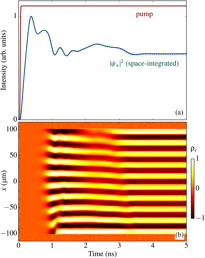
Figure 1: Spin pattern formation in a 1D system. (a) Time dependences of the pump intensity $|f|^{2}$ and the space-integrated cavity-field components $|\psi_{\pm}|^{2}$. (b) Spatiotemporal distribution of the circular-polarization degree $\rho_{c}=(|\psi_{+}|^{2}-|\psi_{-}|^{2})/(|\psi_{+}|^{2}+|\psi_{-}|^{2})$.

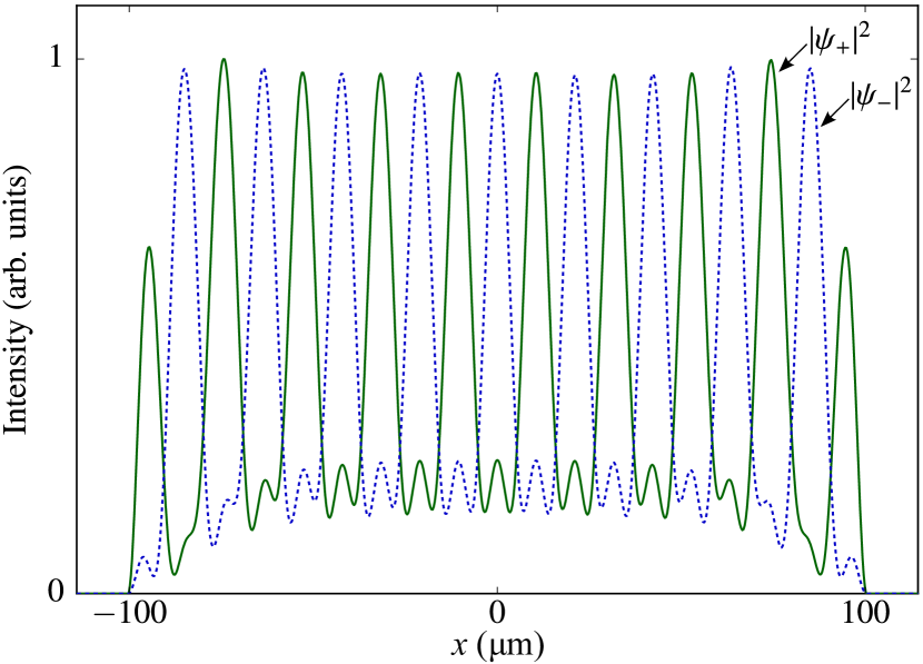
Figure 2: Steady-state patterns in a 1D system. Explicit spatial dependences of $|\psi_{+}|^{2}$ and $|\psi_{-}|^{2}$ at the final stage of the evolution displayed in Fig. 1 ($t\gtrsim 4$ ns).

1D wires.—Let us now turn to a 1D polariton system. On the assumption of a zero exciton-photon detuning, the polariton effective mass $m$ is taken to be twice larger than the photon one: $m=2\epsilon E_{0}/c^{2}$. The ground-state energy $E_{0}=1.5$ eV and dielectric constant $\epsilon=12.5$ are characteristic of GaAs-based microcavities Yamamoto et al. (2000). The free parameters are $\gamma=5\leavevmode\nobreak\ \mu$eV, $g=50\leavevmode\nobreak\ \mu$eV, and $D=35\leavevmode\nobreak\ \mu$eV; they are reachable in state-of-the-art samples and meet the necessary condition obtained previously. The length $L$ of the wire amounts to $200\leavevmode\nobreak\ \mu$m. On its boundaries, the decay rate $\gamma$ is set to increase sharply, so that $\psi_{\pm}$ tend to zero. The considered phenomena are qualitatively independent of $L$, provided it is large enough.

Figure 1 represents the obtained solution. The integral values of $|\psi_{+}|^{2}$ and $|\psi_{-}|^{2}$ evolve synchronously [Fig. 1(a)]. However, the spin-up and spin-down fractions of the field get separated in space in nearly 0.5 ns after the pump has been switched on. A comparatively slow self-organization process, which takes the following 2 ns, results in a periodic spin distribution [Fig. 1(b)]. Figure 2 shows the finally established spatial dependences of $|\psi_{+}|^{2}$ and $|\psi_{-}|^{2}$. They are not mutually equivalent, which is an artifact of finite $L$, however, they have the same integral intensities. The sites with high degrees of circular polarization have comparatively high intensities and are separated from each other by weakly populated zones.

The size $a$ of the spin domains is connected with their momentum-space width that, in turn, is limited in accordance with the energy and momentum conservation laws. On the assumption that the two-particle breakup of the driven mode $(0,0)\to(k,-k)$ is the only scattering process, we have $\hbar_{\vphantom{m}}^{2}k_{\mathrm{max}}^{2}/2m=D+g/2$. Then the following rough estimate is derived: $a_{\mathrm{min}}\approx 2/k_{\mathrm{max}}=2\hbar/\sqrt{2m(D+g/2)}\approx 6\leavevmode\nobreak\ \mu$m, which turns out to be only moderately smaller than the actual size of the domains seen in Fig. 2 (${\sim}\,10\leavevmode\nobreak\ \mu$m).

Notice that in the “spinless” system continuously driven at $k=0$ all steady states must be homogeneous Gavrilov (2014); Gavrilov et al. (2015). In our system, homogeneous solutions are forbidden. Stability can be reached only when all inhomogeneities are balanced, which implies a periodic spatial distribution of the field. Then all spin states separated by the lattice period ($2a$) have the same intensity and phase and are thereby synchronized at each given time moment. However, in a different parameter area some or many of them fall out of synchronization even at $t\to\infty$, so that the entire system never comes to stability.

Why the spin chains are chimera states?—The spontaneous breaking of spatial symmetry is a well-known phenomenon. Usually it is understood in view of extremal principles, when, for instance, pattern formation minimizes the free energy of the system. After the system has reached the global minimum, its collective states are asymptotically stable and described by order parameters Haken (1975). In this respect dynamical chimeras are essentially more complex. In terms of oscillator networks, they contain both synchronized (coherent) and desynchronized (incoherent) parts Panaggio and Abrams (2015). Only in the limiting cases chimeras may collapse into fully ordered states or become fully turbulent; such transitions have recently been observed in lasers Larger et al. (2015). It is difficult to define a quantity that could serve as a measure of stability of chimeras in the general case. The persistence of the irregular part makes the usual definition of stability inapplicable. On the other hand, chimera states are shown to be statistically robust against random structural perturbations even when the regular part is nearly absent Yao et al. (2013).

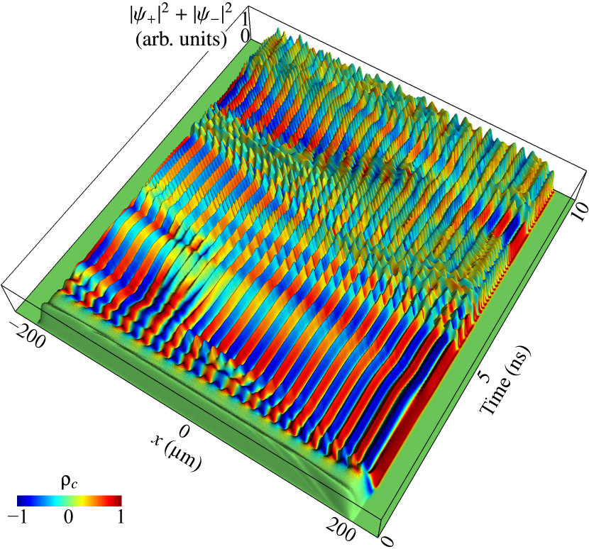
Figure 3: Formation of a nonstatic chimera in a 1D polariton wire.

Formation of a nonstatic chimera is shown in Fig. 3. This example is somewhat untypical in that it combines several dynamical regimes which in their pure states are observed in separate parameter areas. Compared to Fig. 1, the calculation is performed for a spatially longer wire with $L=400\leavevmode\nobreak\ \mu$m. The pump $f^{2}$ is nearly twice stronger; it is turned on in several tens of picoseconds and then held constant.

At the first stage the field arranges itself into a set of opposite-spin domains. Soon after that it behaves more regularly but exhibits occasional jumps at certain spatial locations. The perturbations propagate in space and usually decay with time; the same effect is also seen in Fig. 1. On the other hand, the spatiotemporal defects can also give birth to freely propagating—solitonic—perturbations of the periodic structure. (Previously, solitons were shown to emerge in the presence of an artificial periodic potential induced by surface acoustic waves Cerda-Méndez et al. (2013).) A typical soliton arrives at $x=+200\leavevmode\nobreak\ \mu$m by $t=5$ ns. Solitons also involve local oscillations within the spin domains they are traveling through; this brings about soliton trains Strecker et al. (2002). Multiplying solitons pave the way for turbulence, however, the system also shows space and time intervals of comparatively regular (synchronized) evolution, which is referred to as intermittency, a halfway point before real chaos Bohr et al. (1998).

This particular example does not end up with full turbulence; in the future the system behaves similarly to what is seen in the interval from 5 to 10 ns. The chimera state remains partially ordered in spite of all internal perturbations, yet it never becomes static. In the general case, the first-order spatial correlation function $\mathfrak{g}(d,t)$, which depends on spatial interval $d$ and time moment $t$, can be less than 1 even for $d=2a$ and $t\to\infty$. Various static and nonstatic chimera states and, in particular, their route from perfect periodicity to turbulence upon varying system parameters, are systematized in Appendix.

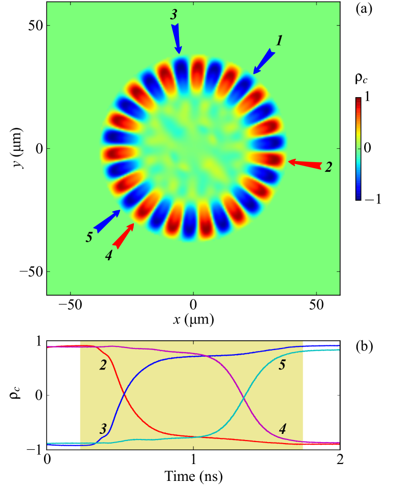
Figure 4: (a) Established spin distribution in a homogeneous 2D cavity under ring-shaped excitation. (b) Controlled spin inversion in reference granules 2–5. The additional laser pulse is focused into a $\mu$m-sized spot at position 1; it has right circular polarization and acts within the shadowed time interval.

2D wires.—In general, the system does not have to be strictly one-dimensional to achieve spin granulation. The periodic patterns occur equally well in homogeneous 2D cavities, given that only a narrow (several $\mu$m wide) spatial stripe is pumped from the outside. A characteristic example is shown in Fig. 4(a). The pump has a ring shape, specifically, $f_{+}(r)=f_{-}(r)\propto e^{-(r-R)^{2}/2w^{2}}$, where $R=30\leavevmode\nobreak\ \mu$m and $w=5\leavevmode\nobreak\ \mu$m. The system parameters are $\gamma=20\leavevmode\nobreak\ \mu$eV, $g=200\leavevmode\nobreak\ \mu$eV, $D=150\leavevmode\nobreak\ \mu$eV. As expected, the established solution breaks rotational invariance of the model.

Strong long-range order.—Two aspects of long-range ordering should be distinguished. The first is predictability: if one knows which of two spin states is enhanced at a certain location, all other sites are thereby also determined. The second aspect is reduced to the question of whether an external control over one given spin state can help manipulate the others. The answer depends on the character of the interaction between spatially separated spins. In our system, the inter-particle repulsion is definitely local, so one might suppose, on one hand, that the effect of an externally created irregularity of the periodic structure should decay with increasing distance. On the other hand, self-organization means that all irregularities are subject to the “enslaving” (Haken (1975)) forces that keep the system ordered and may even reorder it in response to changing environment.

The above considerations lead one to the idea of the following numerical experiment. Let us take the established system represented by Fig. 4(a) and perturb it with an additional pump beam focused into a $1\leavevmode\nobreak\ \mu$m spot in such a way that the spin of a particular granule is reversed. The intensity of this beam becomes negligible already in a few microns away from the target granule so that it cannot affect remote locations directly. The calculations show that after a comparatively short-term perturbation the spin granules are restored in precisely the same states and positions. If, by contrast, the pulse is long enough, then all of the spin states get reversed one after another; and after the local pulse has gone they remain steady.

In Fig. 4(a), the granule whose spin is to be reversed manually is labeled “1”. Labels 2–5 mark the reference sites whose future dynamics (circular-polarization degree vs. time) is explicitly depicted in Fig. 4(b); the time span of the additional local pulse is shadowed. It is seen that comparatively nearby granules 2 and 3 get reversed in about 0.3 ns, whereas the switches of 4 and 5 take ${\sim}\,1$ ns longer. As a result, all spin states are reversed in due order, which constitutes a basic prototype of information transmission.

The considered phenomena strongly depend on transverse dimension $w$. At large $w$ the field is aperiodic and usually takes the shape of chaotically placed filaments Gavrilov (2016) resembling turbulent liquids. Such systems are long-ordered, but they cannot be manipulated predictably. On the contrary, decreasing $w$ involves strong ordering in the form of a stiff but not necessarily static spin network.

Conclusion.—In summary, it is predicted that resonantly driven systems of locally interacting bosons can form chimera states which are different from both the Kuramoto networks (Kuramoto and Battogtokh (2002); Abrams and Strogatz (2004); Acebrón et al. (2005)) and lasers with dime-delayed feedback (Larger et al. (2013, 2015)). Driven and dissipative Bose systems are shown to rid themselves of strict phase locking with respect to the driving field, which can result in strong internal ordering and bright solitons propagating in spontaneously formed periodic domain structures. Unlike quasi-equilibrium Bose condensates, the “incoherent” part of a polariton chimera state has purely dynamical nature; the system is not coupled to a thermal reservoir and thus can be manipulated immediately by optical means.

APPENDIX

Here we systematize the chimera states formed in 1D polariton wires. In particular, transition from static periodic patterns to disordered states is illustrated.

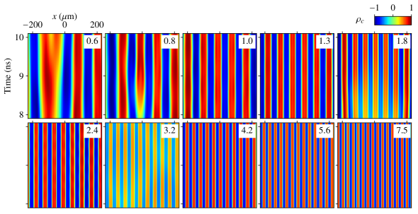
Figure 5: Chimera states in a polariton wire at different $\gamma$ and fixed ratios $g/\gamma=5$, $D/\gamma=4$. Numbers indicate $\gamma$ in $\mu$eV; they form a geometric progression, $\gamma_{n}=\frac{4}{3}\gamma_{n-1}$. For each figure, the pump intensity is set near the instability threshold $f_{\mathrm{thr}}^{2}(\gamma,g,D)$. Color scale represents $\rho_{c}$.

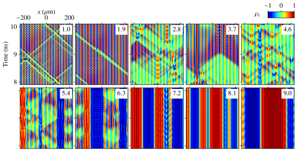
Figure 6: Chimera states at different pump intensities $f^{2}$ above the instability threshold $f_{\mathrm{thr}}^{2}$. Numbers indicate the ratio $f^{2}/f_{\mathrm{thr}}^{2}$. Parameters are $\gamma=10\leavevmode\nobreak\ \mu$eV, $D=g=5\gamma$. Color scale represents the degree of circular polarization $\rho_{c}$.

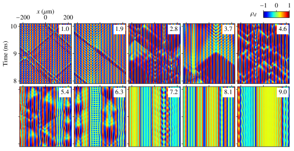
Figure 7: The same series as in Fig. 6, except that color scale represents the degree of the $\pm 45^{\circ}$ linear polarization $\rho_{d}$ [see Eq. (7)].

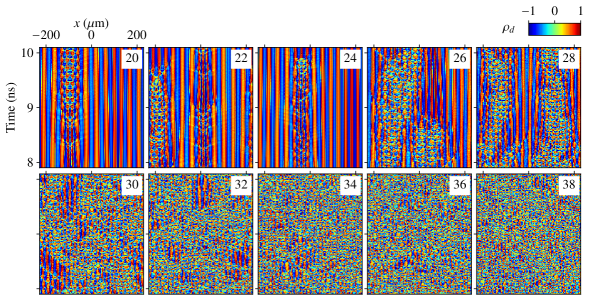
Figure 8: Chimera states at different $D=g$ and constant $\gamma=5\leavevmode\nobreak\ \mu$eV. Numbers indicate $g/\gamma$. For each figure, the pump intensity is set in the middle of the instability interval. Color scale represents  $\rho_{d}$.

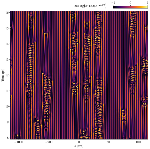
Figure 9: Cosine of the phase difference between $\psi_{+}$ and the driving field. All system parameters are exactly the same as in Fig. 8 ($g/\gamma=24$) except that the wire is now 5 times longer, $L\approx 2.3$ mm.

Chimeras appear when the energy splitting $g=E_{x}-E_{y}$ of the polariton eigenstates exceeds their linewidths $\gamma$ by a factor of 4 or greater. The pump frequency $E_{p}/\hbar$ should be chosen in such a way that detuning $D=E_{p}-E_{0}=E_{p}-(E_{x}+E_{y})/2$ is comparable to $g$, specifically, $g/2\lesssim D\lesssim 2g$. The pump polarization should match the upper sublevel, so that $f_{+}=f_{-}$, $f_{x}^{2}=2f_{+}^{2}$, and $f_{y}=0$; this requirement is not very stiff though. Then a finite interval of $f^{2}\equiv f_{x}^{2}$ exists in which no homogeneous solutions of the form $\psi_{\pm}(x,t)=\bar{\psi}_{\pm}e^{-iE_{p}t/\hbar}$ remain stable, be they spin-symmetric ($\bar{\psi}_{+}=\bar{\psi}_{-}$) or highly asymmetric ($|\bar{\psi}_{\pm}|\ll|\bar{\psi}_{\mp}|$). In general, this is valid only up to $g/\gamma\sim 50$; a further increase of $g/\gamma$ would lead to a new kind of plane-wave multistability which is not discussed here.

To exclude any transitional effects as much as possible, here and in what follows we consider the evolution interval starting 8 ns after the constant pump has been turned on, which exceeds all characteristic times of the discussed system (e. g., $\hbar/\gamma$). The boundary conditions are periodic, which allows one to exclude edge effects.

First, let us demonstrate how to control the size of the spin granules and, thus, the network period. In the main part of the article we have argued that the minimum size $a_{\mathrm{min}}$ should be sensitive to the effective mass and pump energy detuning, namely, $a_{\mathrm{min}}\approx 2\hbar/\sqrt{2m(D+g/2)}$. In the series displayed in Fig. 5, parameters $D$, $g$, and $\gamma$ are successively increased, while the ratios $D/\gamma=4$ and $g/\gamma=5$ are held constant. The chosen values of $\gamma$ (in $\mu$eV) are indicated in each subplot, they form a geometric progression $\gamma_{n}=\frac{4}{3}\,\gamma_{n-1}$. The color scheme represents the circular-polarization degree,

$$\rho_{c}=\frac{\psi_{+}^{*}\psi_{+}^{\vphantom{*}}-\psi_{-}^{*}\psi_{-}^{\vphantom{*}}}{\psi_{+}^{*}\psi_{+}^{\vphantom{*}}+\psi_{-}^{*}\psi_{-}^{\vphantom{*}}},$$ (6)

as a function of time (within a 2 ns interval) and spatial coordinate. The pump was set near the threshold $f^{2}\gtrapprox f_{\mathrm{thr}}^{2}(\gamma,g,D)$ for each subplot, which results in nearly static (collapsed) chimera states. As expected, the network period $a$ successively decreases.

To obtain nonstatic chimera states, one should to increase field density. Figure 6 shows the solutions obtained at different pump densities $f^{2}$ above the instability threshold $f_{\mathrm{thr}}^{2}$. With increasing $f$ the dynamics becomes less regular, and bright solitons that usually propagate at constant velocities in perfectly periodic networks become untypical. Instead, different spin domains merge and form synchronized clusters. This series does not come to turbulence, because at $f^{2}/f_{\mathrm{thr}}^{2}\gtrapprox 9$ the instability interval terminates and the system comes back to plane-wave multistability; only one “cluster” with a spontaneously chosen but constant polarization remains afterwards.

The following Fig. 7 shows exactly the same series, but color now represents the degree of the $\pm 45^{\circ}$ linear polarization (sometimes referred to as the third Stokes parameter),

$$\rho_{d}=\frac{\psi_{x}^{*}\psi_{y}^{\vphantom{*}}+\psi_{y}^{*}\psi_{x}^{\vphantom{*}}}{\psi_{x}^{*}\psi_{x}^{\vphantom{*}}+\psi_{y}^{*}\psi_{y}^{\vphantom{*}}},$$ (7)

where $\psi_{\pm}=(\psi_{x}\mp i\psi_{y})/\sqrt{2}$ by definition. Comparison of Figs. 6 and 7 makes clear that spin-periodic chimera states also show a sort of bistability: for instance, the spin-up domains have either nearly circular ($\rho_{c}\sim 1$) or “diagonal” linear polarization ($\rho_{d}\sim 1$) and occasionally switch between these two states. Solitons propagating through a network with high $|\rho_{c}|$ have high $|\rho_{d}|$ and vice versa. At the same time, the sign of $\rho_{c}$ equals the sign of $\rho_{d}$ at each site and usually remains constant.

Let us now discuss the route to turbulence. As said above, a mere increase of the pump intensity would only drive the system beyond the zone of chimeras and thus make it stable again. Now we fix the decay rate $\gamma=5\leavevmode\nobreak\ \mu$eV and increase both $g$ and $D=g$ (Fig. 8). For each $g$, the pump density is set in the middle of the instability interval. It is seen that the field eventually comes to a strongly disordered state. The intervals of a regular evolution become occasional insertions in a turbulent phase. The spatial extent and duration of such intervals gradually decrease, and eventually they get dissolved completely. This is an instance of the intermittent transition to turbulence whose low-dimensional prototype was found in the Lorenz system [Commun. Math. Phys. 74, 189 (1980)].

The intermittent solutions turn out to be analogous to discrete oscillator networks. Indeed, a wire of length $L$ exhibits $N=L/a$ peaks of the field density. In a steady state the chain is periodic: all co-polarized peaks share the same phase and, thus, are perfectly synchronized. Increasing density makes them fluctuate, and their synchronization becomes imperfect (yet still strong). However, with increasing $g/\gamma$, a number of sites completely fall out of synchronization for quite a long time but occasionally come back, which is seen in Fig. 9 representing the phase dynamics explicitly. The desynchronized domains look like impurities in a periodic lattice, and they hamper signal transmission. Their average number per unit length is nearly constant in time and independent of $N$ (at $N\to\infty$), which is an important feature of the Kuramoto networks. Surprisingly, here a similar network is shown to arise out of a homogeneous system of locally interacting bosons.

References

- Panaggio and Abrams (2015) M. J. Panaggio and D. M. Abrams, Nonlinearity 28, R67 (2015).
- Kuramoto and Battogtokh (2002) Y. Kuramoto and D. Battogtokh, Nonlinear Phenom. Complex Syst. 5, 380 (2002).
- Abrams and Strogatz (2004) D. M. Abrams and S. H. Strogatz, Phys. Rev. Lett. 93, 174102 (2004).
- Acebrón et al. (2005) J. A. Acebrón, L. L. Bonilla, C. J. Pérez Vicente, F. Ritort, and R. Spigler, Rev. Mod. Phys. 77, 137 (2005).
- Larger et al. (2015) L. Larger, B. Penkovsky, and Y. Maistrenko, Nat Commun 6, 7752 (2015).
- Larger et al. (2013) L. Larger, B. Penkovsky, and Y. Maistrenko, Phys. Rev. Lett. 111, 054103 (2013).
- Martens et al. (2013) E. A. Martens, S. Thutupalli, A. Fourrière, and O. Hallatschek, Proc. Natl Acad. Sci. USA 110, 10563 (2013).
- Tinsley et al. (2012) M. R. Tinsley, S. Nkomo, and K. Showalter, Nat Phys 8, 662 (2012).
- Andrzejak et al. (2016) R. G. Andrzejak, C. Rummel, F. Mormann, and K. Schindler, Scientific Reports 6, 23000 (2016).
- Weisbuch et al. (1992) C. Weisbuch, M. Nishioka, A. Ishikawa, and Y. Arakawa, Phys. Rev. Lett. 69, 3314 (1992).
- Yamamoto et al. (2000) Y. Yamamoto, T. Tassone, and H. Cao, Semiconductor Cavity Quantum Electrodynamics (Springer-Verlag, 2000).
- Elesin and Kopaev (1973) V. F. Elesin and Y. V. Kopaev, Sov. Phys. JETP 36, 767 (1973).
- Haug and Kranz (1983) H. Haug and H. H. Kranz, Zeitschrift für Physik B Condensed Matter 53, 151 (1983).
- Kavokin et al. (2007) A. V. Kavokin, J. J. Baumberg, G. Malpuech, and P. Laussy, Microcavities (Oxford University Press, 2007).
- Sarkar et al. (2010) D. Sarkar, S. S. Gavrilov, M. Sich, J. H. Quilter, R. A. Bradley, N. A. Gippius, K. Guda, V. D. Kulakovskii, M. S. Skolnick, and D. N. Krizhanovskii, Phys. Rev. Lett. 105, 216402 (2010).
- Adrados et al. (2010) C. Adrados, A. Amo, T. C. H. Liew, R. Hivet, R. Houdré, E. Giacobino, A. V. Kavokin, and A. Bramati, Phys. Rev. Lett. 105, 216403 (2010).
- Kammann et al. (2012) E. Kammann, T. C. H. Liew, H. Ohadi, P. Cilibrizzi, P. Tsotsis, Z. Hatzopoulos, P. G. Savvidis, A. V. Kavokin, and P. G. Lagoudakis, Phys. Rev. Lett. 109, 036404 (2012).
- Antón et al. (2015) C. Antón, S. Morina, T. Gao, P. S. Eldridge, T. C. H. Liew, M. D. Martín, Z. Hatzopoulos, P. G. Savvidis, I. A. Shelykh, and L. Viña, Phys. Rev. B 91, 075305 (2015).
- Cilibrizzi et al. (2016) P. Cilibrizzi, H. Sigurdsson, T. C. H. Liew, H. Ohadi, A. Askitopoulos, S. Brodbeck, C. Schneider, I. A. Shelykh, S. Höfling, J. Ruostekoski, and P. Lagoudakis, Phys. Rev. B 94, 045315 (2016).
- Solnyshkov et al. (2009) D. D. Solnyshkov, R. Johne, I. A. Shelykh, and G. Malpuech, Phys. Rev. B 80, 235303 (2009).
- Shelykh et al. (2008a) I. A. Shelykh, D. D. Solnyshkov, G. Pavlovic, and G. Malpuech, Phys. Rev. B 78, 041302 (2008a).
- Shelykh et al. (2008b) I. A. Shelykh, T. C. H. Liew, and A. V. Kavokin, Phys. Rev. Lett. 100, 116401 (2008b).
- Gavrilov et al. (2012) S. S. Gavrilov, A. S. Brichkin, A. A. Demenev, A. A. Dorodnyy, S. I. Novikov, V. D. Kulakovskii, S. G. Tikhodeev, and N. A. Gippius, Phys. Rev. B 85, 075319 (2012).
- Sekretenko et al. (2013a) A. V. Sekretenko, S. S. Gavrilov, S. I. Novikov, V. D. Kulakovskii, S. Höfling, C. Schneider, M. Kamp, and A. Forchel, Phys. Rev. B 88, 205302 (2013a).
- Gavrilov and Kulakovskii (2016) S. S. Gavrilov and V. D. Kulakovskii, JETP Letters 104, 827 (2016).
- Gavrilov (2016) S. S. Gavrilov, Phys. Rev. B 94, 195310 (2016).
- Liew et al. (2008) T. C. H. Liew, A. V. Kavokin, and I. A. Shelykh, Phys. Rev. Lett. 101, 016402 (2008).
- Johne et al. (2009) R. Johne, N. S. Maslova, and N. A. Gippius, Solid State Communications 149, 496 (2009).
- Gavrilov and Gippius (2012) S. S. Gavrilov and N. A. Gippius, Phys. Rev. B 86, 085317 (2012).
- Gavrilov et al. (2014a) S. S. Gavrilov, A. A. Demenev, and V. D. Kulakovskii, JETP Letters 100, 817 (2014a).
- Ciuti et al. (1998) C. Ciuti, V. Savona, C. Piermarocchi, A. Quattropani, and P. Schwendimann, Phys. Rev. B 58, 7926 (1998).
- Vladimirova et al. (2010) M. Vladimirova, S. Cronenberger, D. Scalbert, K. V. Kavokin, A. Miard, A. Lemaître, J. Bloch, D. Solnyshkov, G. Malpuech, and A. V. Kavokin, Phys. Rev. B 82, 075301 (2010).
- Sekretenko et al. (2013b) A. V. Sekretenko, S. S. Gavrilov, and V. D. Kulakovskii, Phys. Rev. B 88, 195302 (2013b).
- Baas et al. (2004) A. Baas, J. P. Karr, H. Eleuch, and E. Giacobino, Phys. Rev. A 69, 023809 (2004).
- Gippius et al. (2007) N. A. Gippius, I. A. Shelykh, D. D. Solnyshkov, S. S. Gavrilov, Y. G. Rubo, A. V. Kavokin, S. G. Tikhodeev, and G. Malpuech, Phys. Rev. Lett. 98, 236401 (2007).
- Gavrilov et al. (2010) S. S. Gavrilov, N. A. Gippius, S. G. Tikhodeev, and V. D. Kulakovskii, JETP 110, 825 (2010).
- Paraïso et al. (2010) T. K. Paraïso, M. Wouters, Y. Léger, F. Morier-Genoud, and B. Deveaud-Plédran, Nat Mater 9, 655 (2010).
- Gavrilov et al. (2013) S. S. Gavrilov, A. V. Sekretenko, S. I. Novikov, C. Schneider, S. Höfling, M. Kamp, A. Forchel, and V. D. Kulakovskii, Appl. Phys. Lett. 102, 011104 (2013).
- Gavrilov et al. (2014b) S. S. Gavrilov, A. S. Brichkin, S. I. Novikov, S. Höfling, C. Schneider, M. Kamp, A. Forchel, and V. D. Kulakovskii, Phys. Rev. B 90, 235309 (2014b).
- Gavrilov (2017) S. S. Gavrilov, JETP Letters 105, 200 (2017).
- Bogolyubov (1947) N. N. Bogolyubov, Izv. Akad. Nauk SSSR, Ser. Fiz. 11, 77 (1947).
- Gavrilov (2014) S. S. Gavrilov, Phys. Rev. B 90, 205303 (2014).
- Gavrilov et al. (2015) S. S. Gavrilov, A. S. Brichkin, Y. V. Grishina, C. Schneider, S. Höfling, and V. D. Kulakovskii, Phys. Rev. B 92, 205312 (2015).
- Haken (1975) H. Haken, Rev. Mod. Phys. 47, 67 (1975).
- Yao et al. (2013) N. Yao, Z.-G. Huang, Y.-C. Lai, and Z.-G. Zheng, Scientific Reports 3, 3522 (2013).
- Cerda-Méndez et al. (2013) E. A. Cerda-Méndez, D. Sarkar, D. N. Krizhanovskii, S. S. Gavrilov, K. Biermann, M. S. Skolnick, and P. V. Santos, Phys. Rev. Lett. 111, 146401 (2013).
- Strecker et al. (2002) K. E. Strecker, G. B. Partridge, A. G. Truscott, and R. G. Hulet, Nature 417, 150 (2002).
- Bohr et al. (1998) T. Bohr, M. H. Jensen, G. Paladin, and A. Vulpiani, Dynamical Systems Approach to Turbulence (Cambridge University Press, 1998).