On the origin of the hard X-Ray excess of high-synchrotron-peaked BL Lac object Mrk 421
Abstract
For the first time, Kataoka & Stawarz reported a clear detection of a hard X-ray excess, above 20 keV, in the high-synchrotron-peaked BL Lac object Mrk 421. We find that this feature may not be produced by the low-energy part of the same electron population that produced the Fermi/LAT -ray. Because of that it is required that the power-law electron energy go down to , which predicts a very strong radio emission (radio flux larger than the observed) even considering the synchrotron self-absorption effect. We investigate the possibility of this excess being produced from the spine/layer jet structure, which has been clearly detected in Mrk 421. We find that (1) similar to one-zone modeling, the spine emissions provide good modeling of the broadband spectral energy distribution, except for the hard X-ray excess; and (2) the hard X-ray excess can be well represented by the synchrotron photons (from the layer) being inverse Compton scattered by the spine electrons.
1 Introduction
Due to the Doppler beaming effect, relativistic jets dominate the broadband emissions (from radio to -ray) of a blazar, in which the viewing angle between the jet direction and line of sight is very small (Blandford & Rees, 1978; Urry & Padovani, 1995). The broadband spectral energy distributions (SEDs) of blazars usually show two significant bumps. One of these peaks at infrared (IR) to X-ray bands, which is believed to be the synchrotron emissions of energetic electrons within the jet. The second bump peaks at the -ray band, which may be the inverse Compton (IC) emissions of the same distribution of electrons emitting the synchrotron bump (e.g., Maraschi et al., 1992; Bloom & Marscher, 1996; Sikora et al., 1994; Dermer & Schlickeiser, 1993, see also the hadronic model: Mannheim (1993); Aharonian (2000); Atoyan & Dermer (2003); Mücke et al. (2003)).
The distribution of the synchrotron peak frequency, , forms a continuous sequence, although the objects usually classified as high-synchrotron-peaked (HSP; Hz), intermediate-synchrotron-peaked (ISP; Hz Hz), and low-synchrotron-peaked (LSP; Hz) blazars, depending on the location of (Abdo et al., 2010). The synchrotron and IC components usually cross at roughly the X-ray band. Therefore, for HSP blazars, the X-ray is usually dominated by softer synchrotron emissions. For most LSP blazars, the X-ray is almost dominated by harder IC emissions. For ISP blazars (and some LSP blazars), the X-ray is a mixture of synchrotron and IC emissions; therefore, the X-ray spectra sometimes show a concave shape in the frame.
The SED modeling is a powerful tool for studying jet physics (see, e.g., Ghisellini & Tavecchio, 2009; Ghisellini et al., 2010, 2014). The lowest-energy electrons are the most plentiful and sensitive to probe the total content of particles in the jet, including the estimated jet power, the particle acceleration mechanism, etc. However, it is very difficult to use radio observation to constrain this minimal electron energy, even though the synchrotron emissions are precisely at the radio band. This is because the synchrotron emissions are likely self-absorbed at the radio band111The observed radio flux is probably the superimposed emissions of many outside optically thick emission regions (e.g., Blandford & Königl, 1979; Ghisellini et al., 1985).. These lowest-energy electrons will IC scatter the soft seed photons and emit at the X-ray band. Therefore, careful SED modeling (especially modeling the IC X-ray spectra) is widely used to estimate the minimal electron energy and furthermore to calculate, for example, the jet power (see, e.g., Celotti & Ghisellini, 2008; Chen et al., 2010; Kang et al., 2014; Ghisellini et al., 2014).
As discussed above, the X-ray spectra of LSP blazars and the rising part of the concave X-ray spectra of ISP blazars may be the character of the IC emission. For HSP blazars, soft X-rays are usually dominated by synchrotron emissions. The hard X-rays would be dominated by the low-energy IC emission part. However, due to the limited sensitivity of instruments in this energy range (above 20 keV), we perhaps know the least about this lowest-energy part of the IC component.
Thanks to the hard X-ray energy range of the Nuclear Spectroscopic Telescope Array (NuSTAR; sensitive in 3-79 keV), the low-energy part of the IC component of some HSP blazars can be detected. For the first time, Kataoka & Stawarz (2016) reported a clear detection of a hard X-ray excess (i.e., a concave X-ray spectrum) above 20 keV of the HSP BL Lac object Mrk 421 during the low state (see also PKS 2155-304; Madejski et al., 2016). In this paper, we investigate the possibilities for the origin of this hard X-ray excess. In Section 2, the general properties of Mrk 421 are presented (especially the detection of the hard X-ray excess). Section 3 provides a detailed discussion of the possible origins of this excess. Section 4 shows a spine/layer model, which can represent the hard X-ray excess. The discussion and conclusion are presented in Section 5.
2 The hard X-Ray excess of Mrk 421
Mrk 421 is a typical HSP source, the first BL Lac object deteced by the Energetic Gamma Ray Experiment Telescope (EGRET, Lin et al., 1992) at energy above 100 MeV and the first extragalactic source detected by imaging atmospheric Cherenkov telescopes (IACTs) at very high energy (VHE; 100 GeV, Punch et al., 1992). It is so bright that it can be detected by modern IACTs within several minutes (Aleksić et al., 2015). Its X-ray and TeV emissions often show well-correlated variability, as do its optical and GeV emissions (e.g., Bartoli et al., 2016; Kapanadze et al., 2016; Ahnen et al., 2016; Sinha et al., 2016). Including -rays, its broadband SED can be well fitted by a one-zone synchrotron self-Compton (SSC) model (e.g., Cao & Wang, 2013; Zheng et al., 2014; Zhu et al., 2016; Baloković et al., 2016). Gorham et al. (2000) estimated the central black hole mass of order based on the imagery and broadline velocity dispersion. Its synchrotron component peaks at the hard X-ray band during the bright state and moves to the soft X-ray band when the source gets fainter (Baloković et al., 2016). During the faintest state in MJD 56302, its synchrotron component peaks at too low a frequency to make it similar to ISP/LSP. Very recently, Kataoka & Stawarz (2016) reported the detection of a significant excess above 20 keV through NuSTAR observations at this faintest epoch (see also the BeppoSAX observation; e.g., Fossati et al., 1999, 2000).
3 The origin of the hard X-Ray excess
Kataoka & Stawarz (2016) compared the spectra of the hard X-ray excess with the simultaneous222The Fermi/LAT data are accumulated over roughly 1 week time intervals (see Baloković et al., 2016). Fermi/LAT power-law -ray spectra (the photon index ; Baloković et al., 2016). They found that this excess follows the extension of the -ray spectra well; therefore, they argued that this hard X-ray excess must be the low-energy part of the SSC emissions of the same electron population that is producing the Fermi/LAT -ray. Actually, the broadband SED at this epoch had been well fitted by a one-zone SSC model (up to the TeV band but except for the hard X-ray spectra; Baloković et al., 2016). However, it can be seen that the observed hard X-ray excess cannot be reproduced by this one-zone modeling: the modeling underestimates the hard X-ray flux (upper left panel of Figure 13 in Baloković et al., 2016). The most likely possibility seems to be that a minimum electron energy that is too much larger () produces a “cutoff” at the low energy part of the SSC component (i.e., very weak emissions at the hard X-ray band). This means that a smaller would increase the hard X-ray emissions and may represent the observed excess. The value of can be easily estimated when assuming that the hard X-ray emissions follow the power-law extension of the Fermi/LAT -ray spectra.
We assume a one-zone model with a broken-power law electron energy distribution,
| (1) |
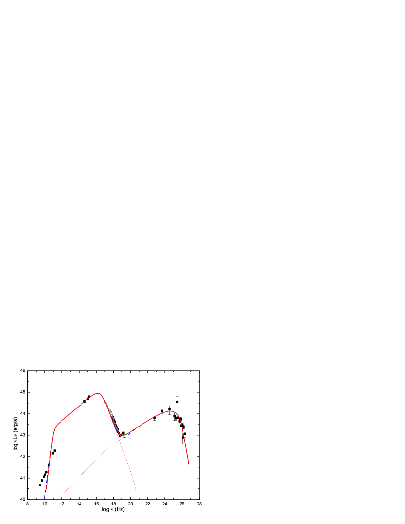
In this model, the power-law distribution electrons below produce the SED from the hard X-ray to the Fermi/LAT -ray emissions through the SSC process (see Baloković et al., 2016). Electrons around will IC synchrotron photons and produce the hard X-ray excess around 20 KeV. We collect this simultaneous broadband SED from Baloković et al. (2016) and Kataoka & Stawarz (2016), which are replotted in Figure 1. The synchrotron and SSC components peak at and Hz, respectively, which correspond to emissions of electrons with energy around . As we know, the Klein-Nishina (KN) effect works at ( is the Doppler beaming factor), and, in this case, the IC (SSC) photon energy approximates . Combining these two formulas, we have . Substituting the observed peak frequencies, we have . This means that the KN effect can only work at peak frequency for a mild Doppler beaming factor (i.e., ), and we have in this case. Such a weak beaming effect seems unexpected for the HSP BL Lac object Mrk 421, because of that it often shows violent emissions and the derived from broadband SED modeling is much larger than this value (e.g., for this epoch’s SED modeling; Baloković et al., 2016). For the case of IC scattering within the Thomsen regime, we have and . Substituting the observed peak frequencies, we have and .
The IC frequency scales as . If emits at Hz and emits at Hz (i.e., the hard X-ray excess above keV), one can estimate . Its synchrotron emissions could extend down to GHz. As disccused in Section 1, the synchrotron emissions are usually synchrotron self-absorbed (SSA) at the radio band; therefore, the predicted radio flux (one-zone model) is usually below the observed one. Now, we will calculate this SSA radio flux (by electrons) and compare it with the observation.
Within the one-zone model, we can easily estimate the jet parameters when provided with a broadband SED (The emission region is assumed to be a homogeneous sphere with radius embedded in a magnetic field with strength ). For a SED at this epoch (Figure 1; see also Baloković et al., 2016; Kataoka & Stawarz, 2016), the spectral indexes below and above the peak frequency are and , respectively (Kataoka & Stawarz, 2016; Abdo et al., 2011; Baloković et al., 2016). The peak luminosities of the synchrotron and SSC bumps are estimated to be and erg s-1, respectively. Combined with the peak frequencies, one can estimate (see e.g., Tavecchio et al., 1998) the magnetic field strength Gs, the normalized electron density , the break energy , the Doppler beaming factor (assumed to be equal to the same value in Baloković et al., 2016), the radius of the emission region cm, and the electron energy indexes below and above the break, and , respectively.
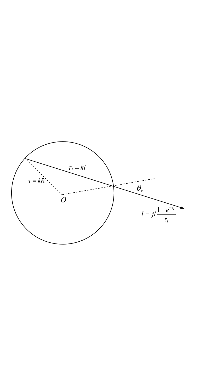
The luminosity in the jet frame is given by (see the Appendix for details; see also Bloom & Marscher, 1996; Kataoka et al., 1999),
| (2) |
where the frequency , the emitting coefficient (-approximation; see the Appendix for details; see also Dermer & Schlickeiser, 2002; Finke et al., 2008)
| (3) |
and the optical depth
| (4) |
where is the Lamer frequency and the is the magnetic field energy density. The prime refers to the value in the jet frame. The frequency and luminosity in the active galactic nucleus (AGN) frame are transformed as and , respectively. The Pico Veleta telescope is used with the EMIR receiver to provide flux measurements at 86.2 GHz and 142.3 GHz (see Figure 1 and Baloković et al., 2016). With the above jet parameters and Equation 4, one can calculate the optical depth (corresponding electron energy ) and () at frequencies of 86.2 and 142.3 GHz, respectively. The expected luminosities (Equation 2) are and erg s-1 at frequencies of 86.2 GHz and 142.3 GHz, respectively. It can be seen that both luminosities are contrary to the observed values, which are lower by 1 order of magnitude (see Figure 1 and Baloković et al., 2016). Even considering the error bar of the input parameters (i.e., the input peak luminosity and frequency and the spectral indexes), the expected luminosities at these two frequencies are larger than the observed ones. This means that even though the radio emission is SSA, the predicted radio fluxes (one-zone model) are still larger than the observed values, which implies that the electron power-law distribution cannot extend down to such a low energy (i.e., ). This indicates that the hard X-ray excess observed by NuSTAR at MJD 56302 cannot be produced by the low-energy part of the same electron population that produced the Fermi/LAT -rays.
A quantified one-zone SED modeling (synchrotron + SSC), including SSA and KN effects, is necessary to check the above estimation. For the model description, see the Appendix for detail (see also Chen et al., 2012; Kang et al., 2014). During our modeling, the Doppler beaming factor is assumed to be same as that in Baloković et al. (2016), i.e., . For our purposes, the first step is setting the minimal electron energy . The modeling SED curve is presented as the solid red line in Figure 1, and the other parameters are the magnetic field strength Gs, the normalized electron density333It can be seen that the normalized electron density here is significantly smaller than the above estimation. This is due to the fact that the estimation depends significantly on the electron energy index below the break energy, here versus above, while the density at the break energy, , is similar for both. , the break energy , the radius of the emission region cm, the electron energy indexes below and above the break and , and the maximal electron energy . It can be seen that the model can reproduce the hard X-ray excess with this low value of , while it predicts larger radio fluxes than ones observed at 86.2 and 142.3 GHz. The second step is that we increase the value of (keeping the other parameters unchanged) to see whether there is a value that can fit the hard X-ray excess and can also predict a lower radio flux. Two values, and 50, are set in the modeling, and results are shown in Figure 1 as green dotted and blue dashed lines, respectively. It can be seen that even though the value increased to , the predicted radio flux has almost no change due to the SSA effect, while the hard X-ray flux significantly decreases, which cannot represent the observed hard X-ray excess. These results confirm our above estimation that the hard X-ray excess observed by NuSTAR at MJD 56302 cannot be produced by the low-energy part of the same electron population that produced the Fermi/LAT -rays.
For the origin of the hard X-ray excess, another possibility is that this excess is actually the high-energy tail of synchrotron X-ray emissions. This requires a spectral pile-up in electron distribution at the highest energies. Kataoka & Stawarz (2016) discussed this possibility and found that it is unlikely to work. The main reasons are as follows. (1) This high-energy pile-up bump could be achieved when the acceleration timescale equals the radiative-loss timescale at the limit for the perfect confinement of electrons within the emission zone (Stawarz & Petrosian, 2008). However, this scenario predicts a flat power tail at lower electron energies, which is inconsistent with the X-ray observation of Mrk 421. (2) This high-energy tail can also be produced by the electron high-energy pile-up due to the reduction of the IC cross-section in the KN regime (Moderski et al., 2005). However, this requires IC cooling dominating over synchrotron cooling, which is not consistent with the fact that Mrk 421 is almost totally dominated by synchrotron emission.
4 The spine/layer jet
Here, we explore the possibility that the production of this hard X-ray excess is related to the spine/layer jet structure: a fast spine surrounded by a slower layer. The main reason for this choice is that Mrk 421 has been observed having a significant and clear spine/layer structure. In other aspects, the spine/layer structure can produce IC SEDs that are significantly different from those of the one-zone model (see details below and, e.g., Ghisellini et al., 2005; Sikora et al., 2016).
Mrk 421 shows a significant core-jet structure. Very long baseline interferometry (VLBI) observations can reveal a detailed jet structure at pc scale. Along the direction perpendicular to the jet axis, the fractional polarization shows significant double bumps increasing at the jet edges, which implies a spine/layer (also called spine-sheath) structure (Piner et al., 2010; Lico et al., 2014). This structure is supported by the similar distributions of the electron vector position angle (EVPA) and even the flux intensity (the so-called limb brightening; Piner et al., 2010; Lico et al., 2014). The layer component usually moves slower than the spine. The relative opposite motion between the spine and layer will amplify the photon energy density from the spine (layer) in the frame of the layer (spine) and therefore produce a different (enhanced) IC emissions. This model has been widely and successfully used to explain the VHE -ray emissions from radio galaxies and blazars (see, e.g., Ghisellini et al., 2005; Tavecchio & Ghisellini, 2008; Sikora et al., 2016).
The spine/layer model used here is same as that in Ghisellini et al. (2005). For geometry, see Figure 1 in Ghisellini et al. (2005). The layer is assumed to be a hollow cylinder with external radius , internal radius and width in the comoving frame of the layer444Double prime refers to values in the frame of the layer, and prime refers to values in the frame of the spine.. For the cylindrical spine, the radius is and the width is . The spine and layer move with velocities and , respectively, with and as the corresponding Lorentz factors. The relative velocity between the spine and the layer is then . Following Ghisellini et al. (2005), the radiation energy densities are considered as follows,
-
•
In the comoving frame of the layer, the radiation energy density (slightly different from that of Ghisellini et al., 2005, to make sure that the radiation energy density is in the same format as that in the spine). In the frame of the spine, this radiation energy density will be boosted to .
-
•
In the comoving frame of the spine, the radiation energy within the spine is assumed to be . The radiation energy density observed in the frame of the layer will be boosted by but also diluted (since the layer is larger than the spine) by a factor .
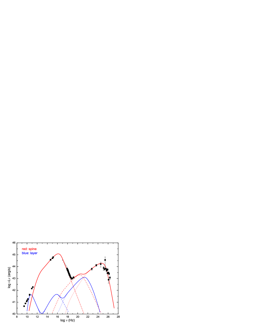
The electron energy distributions in the spine and layer are all assumed to be broken power laws, as expressed in Equation 1, but with different parameters. In our modeling, we always assume , as in Ghisellini et al. (2005). Figure 2 presents our SED modeling result, and the corresponding parameters are listed in Table 1. For the geometry parameters, , , and cm. The red and blue lines represent the spine and layer emissions, respectively. While the dot-dashed lines are the synchrotron emissions, the dotted lines show the SSC emissions, and the dashed lines are for the IC emissions of seed photons originated externally from the layer/spine. It can been seen that, similar to one-zone modeling (Baloković et al., 2016), the synchrotron + SSC emissions of the spine can produce almost a whole SED, except for the hard X-ray excess. This hard X-ray excess can be successfully represented by the process of seed photons (produced from the layer) being IC scattered by the nonthermal electrons within the spine.
| (∘) | (Gs) | |||||||||
|---|---|---|---|---|---|---|---|---|---|---|
| Spine | 2 | 21.4 | 27.5 | 0.23 | 996 | 29009 | 300 | 100 | 2.0 | 5.2 |
| Layer | 2 | 4.7 | 9.1 | 0.0087 | 593 | 326 | 2 | 100 | 1.0 | 5.0 |
5 Discussion and Conclusions
The spine/layer jet model was initially studied by Sol et al. (1989). Such a scenario can explain some inconsistencies between the observations and the AGN standard unified model. Within the standard unified model, radio galaxies and blazars have the same relativistic jets but different viewing angles (Urry & Padovani, 1995). Because of the Doppler beaming factor significantly depending on the viewing angle, one can derive a number distribution as a function of viewing angle; roughly the number ratio between the radio galaxies and blazars. One finds that this number ratio (within the one-zone model) is inconsistent with observations (Chiaberge et al., 2000). This question can be solved if the jet is actually structured, e.g., a faster-moving spine surrounded by a slower-moving layer (Chiaberge et al., 2000). In the spine/layer model, jet emissions with small viewing angles will be dominated by the faster spine (for blazars), while the layer component will contribute more or even dominate the emissions in the case of a larger viewing angle (for radio galaxies). Therefore, in the case of the spine/layer model, one expects a larger number ratio between radio galaxies and blazars compared to the one-zone model (Chiaberge et al., 2000). As discussed above, the relative opposite motion between the spine and the layer will amplify the photon energy density produced from the spine (layer) in the frame of the layer (spine) by (see Section 4). Therefore, one expects that the IC emissions will be enhanced relative to the one-zone model (Ghisellini et al., 2005). This spine/layer model has been widely and successfully used to explain the VHE -ray emissions of radio galaxies and blazars (see, e.g., Ghisellini et al., 2005; Tavecchio & Ghisellini, 2008; Sikora et al., 2016). The orphan flare is an interesting phenomenon in blazar observations. Recently, MacDonald et al. (2015) proposed that, when a faster-moving spine (emission zone) moves across a slower-moving (or steady) layer/ring, the sudden increase of the energy density of external seed photons (produced from the layer) will be IC scattered by the spine electrons and produce an orphan flare in the -ray band (see also MacDonald et al., 2016). The origin of the spine/layer structure is, however, unclear. It could arise directly from a jet launching process in which the external layer is ejected from the accretion disk while the central spine is fueled from the black hole ergosphere, as shown in some numerical simulations (e.g., Mizuno et al., 2007; Meliani et al., 2010). Alternatively, the Kelvin-Helmholtz instability can occur when there is velocity shear in a single continuous fluid, which can create the spine/layer structure seen in 3C 273 (Lobanov & Zensus, 2001). The third possibility is that the falling of the magnetized accretion flow leads to accumulation of the inflating toroidal magnetic field inside the accretion disk, which can produce a magnetic tower jet. The magnetic tower jet presents a central helical magnetic field “spine” surrounded by a reversed magnetic field “sheath,” which could be a prototype of a spine/layer structure (see, e.g., Kato et al., 2004; Li et al., 2006).
For the first time, Kataoka & Stawarz (2016) reported the detection of the hard X-ray excess above 20 keV in the HSP BL Lac object Mrk 421. This feature offers important information for our understanding of jet physics. Many probabilities may account for this excess. However, as discussed above, it cannot be the high-energy tail of the synchrotron X-ray emissions, because the requirement of high-energy pile-up in electron energy distribution cannot be achieved due to the theoretical predictions being in conflict with the observations (the spectral index/Compton dominance; see Section 3 and Kataoka & Stawarz, 2016). Alternatively, it seems to be the low-energy tail of the Fermi/LAT -ray spectra. As discussed in Section 3, this possibility requires the minimal electron energy down to . Such a lower electron energy predicts a very strong radio emission, even with the SSA effect, which is larger than the observed radio flux. Therefore, the hard X-ray excess cannot be the low-energy tail of the Fermi/LAT -ray spectra.
Because of that, Mrk 421 shows a clear spine/layer structure from VLBI observations (e.g., the limb brightening, the double-hump distribution of fractional polarization, and the EPVA along the perpendicular jet direction). We investigate the possibilities of the hard X-ray excess produced related to this structure. We find that the spine emissions provide good-modeling of the broadband SED except for the hard X-ray excess, which is similar to one-zone modeling (see Figure 2 and Baloković et al., 2016). The hard X-ray excess can be well represented by the synchrotron photons from the layer being IC scattered by the spine electrons (see Figure 2). Until now, about 49 HSP BL Lacs555http://tevcat.uchicago.edu/ have been detected that have VHE emissions. The broadband SEDs of some of them can be well fitted by the one-zone model (e.e., Paggi et al., 2009; Zhang et al., 2012; Ghisellini et al., 2014; Yan et al., 2014; Ding et al., 2017). However, it should be noted that these well-modeled SEDs do not include the rising part at the hard X-ray band. If these sources have hard X-ray spectra similar to that of Mrk 421 (i.e., the hard X-ray excess/the concave feature), it can be seen that almost all of these SED modelings underestimate their hard X-ray emissions. Actually, some LSP BL Lacs have a similar question. The LSP BL Lacs present very hard X-ray spectra, which may be the rising part of the second IC component. However, the one-zone SSC model is also much harder to fit to their broadband SEDs (Yan et al., 2014), which are usually modeled by a two-zone model or a one-zone SSC + EC (external Comptoton) model (e.g., Ghisellini et al., 2011; Abdo et al., 2011). For our SED modeling of Mrk 421, it should be noted that the model used is just a simple toy model, i.e., using two distinct regions (spine and layer) instead of continuing the distribution from jet axis to edge, although our modeled parameters are among the typical values of blazars (e.g., Ghisellini et al., 2010, 2014; Zhang et al., 2012).
The HSP BL Lac PKS 2155-304 has also been seen to present a flattened spectrum above the 4 keV during the low state (observations by BeppoSAX, XMM-Newton, and NuSTAR; Giommi et al., 1998; Chiappetti et al., 1999; Zhang, 2008; Madejski et al., 2016). This flattened X-ray spectrum had been considered to be SSC emission of the lowest-energy electrons, and the broadband SED was fitted within the one-zone SSC model by Madejski et al. (2016). The minimal electron energy down to is required to reproduce the hard X-ray feature. Because of that, the jet power significantly depends on the minimal electron energy. Such a small requires a very large jet power (assuming one cold proton per electron), erg s-1, which requires the accretion rate to exceed the Eddington rate, even assuming high efficiency of conversion of the accretion power to jet power (Madejski et al., 2016). As suggested by Sikora et al. (2016), the spine/layer model is less demanding of jet power than the one-zone model and can reproduce the basic features of -ray events. In another aspect, the radio data to compare with the SED modeling of PKS 2155-304 are lacking (see Figure 4 in Madejski et al., 2016).
The jet power of Mrk 421 (including both spine and layer) can be easily calculated when provided with these SED modeling parameters (see Table 1): erg s-1, which is times the jet radiation power (assuming ), and erg s-1, where is the bolometric jet luminosity. Therefore, the jet carries 1.6% of the Eddington luminosity, which is consistent with the fact that HSP BL Lacs (and Mrk 421 in particular) accrete via inefficient, low-accretion-rate, or advection-dominated accretion flow (for a recent overview, see Yuan & Narayan, 2014).
References
- Abdo et al. (2010) Abdo, A. A., Ackermann, M., Ajello, M., et al. 2010, ApJ, 715, 429
- Abdo et al. (2011) Abdo, A. A., Ackermann, M., Ajello, M., et al. 2011, ApJ, 730, 101
- Abdo et al. (2011) Abdo, A. A., Ackermann, M., Ajello, M., et al. 2011, ApJ, 736, 131
- Aharonian (2000) Aharonian, F. A. 2000, New A, 5, 377
- Ahnen et al. (2016) Ahnen, M. L., Ansoldi, S., Antonelli, L. A., et al. 2016, A&A, 593, A91
- Aleksić et al. (2015) Aleksić, J., Ansoldi, S., Antonelli, L. A., et al. 2015, A&A, 576, A126
- Atoyan & Dermer (2003) Atoyan, A. M., & Dermer, C. D. 2003, ApJ, 586, 79
- Baloković et al. (2016) Baloković, M., Paneque, D., Madejski, G., et al. 2016, ApJ, 819, 156
- Bartoli et al. (2016) Bartoli, B., Bernardini, P., Bi, X. J., et al. 2016, ApJS, 222, 6
- Blandford & Königl (1979) Blandford, R. D., & Königl, A. 1979, ApJ, 232, 34
- Blandford & Rees (1978) Blandford, R. D., & Rees, M. J. 1978, BL Lac Objects, 328
- Bloom & Marscher (1996) Bloom, S. D., & Marscher, A. P. 1996, ApJ, 461, 657
- Blumenthal & Gould (1970) Blumenthal, G. R., & Gould, R. J. 1970, Reviews of Modern Physics, 42, 237
- Cao & Wang (2013) Cao, G., & Wang, J. 2013, PASJ, 65, 109
- Celotti & Ghisellini (2008) Celotti, A., & Ghisellini, G. 2008, MNRAS, 385, 283
- Chen et al. (2010) Chen, L., Bai, J.-M., Zhang, J., & Liu, H.-T. 2010, Research in Astronomy and Astrophysics, 10, 707
- Chen et al. (2012) Chen, L., Cao, X., & Bai, J. M. 2012, ApJ, 748, 119
- Chiaberge et al. (2000) Chiaberge, M., Celotti, A., Capetti, A., & Ghisellini, G. 2000, A&A, 358, 104
- Chiappetti et al. (1999) Chiappetti, L., Maraschi, L., Tavecchio, F., et al. 1999, ApJ, 521, 552
- Dermer & Schlickeiser (2002) Dermer, C. D., & Schlickeiser, R. 2002, ApJ, 575, 667
- Dermer & Schlickeiser (1993) Dermer, C. D., & Schlickeiser, R. 1993, ApJ, 416, 458
- Ding et al. (2017) Ding, N., Zhang, X., Xiong, D. R., & Zhang, H. J. 2017, MNRAS, 464, 599
- Finke et al. (2008) Finke, J. D., Dermer, C. D., & Böttcher, M. 2008, ApJ, 686, 181-194
- Fossati et al. (2000) Fossati, G., Celotti, A., Chiaberge, M., & Zhang, Y. H. 2000, American Institute of Physics Conference Series, 510, 313
- Fossati et al. (1999) Fossati, G., Chiappetti, L., Celotti, A., et al. 1999, Nuclear Physics B Proceedings Supplements, 69, 423
- Ghisellini et al. (1985) Ghisellini, G., Maraschi, L., & Treves, A. 1985, A&A, 146, 204
- Ghisellini & Tavecchio (2009) Ghisellini, G., & Tavecchio, F. 2009, MNRAS, 397, 985
- Ghisellini et al. (2005) Ghisellini, G., Tavecchio, F., & Chiaberge, M. 2005, A&A, 432, 401
- Ghisellini et al. (2011) Ghisellini, G., Tavecchio, F., Foschini, L., & Ghirlanda, G. 2011, MNRAS, 414, 2674
- Ghisellini et al. (2010) Ghisellini, G., Tavecchio, F., Foschini, L., et al. 2010, MNRAS, 402, 497
- Ghisellini et al. (2014) Ghisellini, G., Tavecchio, F., Maraschi, L., Celotti, A., & Sbarrato, T. 2014, Nature, 515, 376
- Giommi et al. (1998) Giommi, P., Fiore, F., Guainazzi, M., et al. 1998, A&A, 333, L5
- Gorham et al. (2000) Gorham, P. W., van Zee, L., Unwin, S. C., & Jacobs, C. S. 2000, American Institute of Physics Conference Series, 515, 165
- Kang et al. (2014) Kang, S.-J., Chen, L., & Wu, Q. 2014, ApJS, 215, 5
- Kapanadze et al. (2016) Kapanadze, B., Dorner, D., Vercellone, S., et al. 2016, ApJ, 831, 102
- Kataoka et al. (1999) Kataoka, J., Mattox, J. R., Quinn, J., et al. 1999, ApJ, 514, 138
- Kataoka & Stawarz (2016) Kataoka, J., & Stawarz, Ł. 2016, ApJ, 827, 55
- Kato et al. (2004) Kato, Y., Mineshige, S., & Shibata, K. 2004, ApJ, 605, 307
- Li et al. (2006) Li, H., Lapenta, G., Finn, J. M., Li, S., & Colgate, S. A. 2006, ApJ, 643, 92
- Lico et al. (2014) Lico, R., Giroletti, M., Orienti, M., et al. 2014, A&A, 571, A54
- Lin et al. (1992) Lin, Y. C., Bertsch, D. L., Chiang, J., et al. 1992, ApJ, 401, L61
- Lobanov & Zensus (2001) Lobanov, A. P., & Zensus, J. A. 2001, Science, 294, 128
- Mücke et al. (2003) Mücke, A., Protheroe, R. J., Engel, R., Rachen, J. P., & Stanev, T. 2003, Astroparticle Physics, 18, 593
- MacDonald et al. (2016) MacDonald, N. R., Jorstad, S. G., & Marscher, A. P. 2016, arXiv:1611.09953
- MacDonald et al. (2015) MacDonald, N. R., Marscher, A. P., Jorstad, S. G., & Joshi, M. 2015, ApJ, 804, 111
- Madejski et al. (2016) Madejski, G. M., Nalewajko, K., Madsen, K. K., et al. 2016, ApJ, 831, 142
- Mannheim (1993) Mannheim, K. 1993, A&A, 269, 67
- Maraschi et al. (1992) Maraschi, L., Ghisellini, G., & Celotti, A. 1992, ApJ, 397, L5
- Meliani et al. (2010) Meliani, Z., Sauty, C., Tsinganos, K., Trussoni, E., & Cayatte, V. 2010, A&A, 521, A67
- Mizuno et al. (2007) Mizuno, Y., Hardee, P., & Nishikawa, K.-I. 2007, ApJ, 662, 835
- Moderski et al. (2005) Moderski, R., Sikora, M., Coppi, P. S., & Aharonian, F. 2005, MNRAS, 363, 954
- Paggi et al. (2009) Paggi, A., Massaro, F., Vittorini, V., et al. 2009, A&A, 504, 821
- Piner et al. (2010) Piner, B. G., Pant, N., & Edwards, P. G. 2010, ApJ, 723, 1150
- Punch et al. (1992) Punch, M., Akerlof, C. W., Cawley, M. F., et al. 1992, Nature, 358, 477
- Rybicki & Lightman (1979) Rybicki, G. B., & Lightman, A. P. 1979, New York, Wiley-Interscience, 1979. 393 p.,
- Sikora et al. (1994) Sikora, M., Begelman, M. C., & Rees, M. J. 1994, ApJ, 421, 153
- Sikora et al. (2016) Sikora, M., Rutkowski, M., & Begelman, M. C. 2016, MNRAS, 457, 1352
- Sinha et al. (2016) Sinha, A., Shukla, A., Saha, L., et al. 2016, A&A, 591, A83
- Sol et al. (1989) Sol, H., Pelletier, G., & Asseo, E. 1989, MNRAS, 237, 411
- Stawarz & Petrosian (2008) Stawarz, Ł., & Petrosian, V. 2008, ApJ, 681, 1725-1744
- Tavecchio & Ghisellini (2008) Tavecchio, F., & Ghisellini, G. 2008, MNRAS, 385, L98
- Tavecchio et al. (1998) Tavecchio, F., Maraschi, L., & Ghisellini, G. 1998, ApJ, 509, 608
- Urry & Padovani (1995) Urry, C. M., & Padovani, P. 1995, PASP, 107, 803
- Yan et al. (2014) Yan, D., Zeng, H., & Zhang, L. 2014, MNRAS, 439, 2933
- Yuan & Narayan (2014) Yuan, F., & Narayan, R. 2014, ARA&A, 52, 529
- Zhang et al. (2012) Zhang, J., Liang, E.-W., Zhang, S.-N., & Bai, J. M. 2012, ApJ, 752, 157
- Zhang (2008) Zhang, Y. H. 2008, ApJ, 682, 789-797
- Zheng et al. (2014) Zheng, Y. G., Kang, S. J., & Li, J. 2014, MNRAS, 442, 3166
- Zhu et al. (2016) Zhu, Q., Yan, D., Zhang, P., et al. 2016, MNRAS, 463, 4481
Appendix A One-zone SSC model
The one-zone SSC model adopted in this paper assumes a homogeneous and isotropic emission region, which is a sphere with radius that has a uniform magnetic field with strength and a uniform electron energy distribution as described by Equation 1. The emission region moves relativistically with a Lorentz factor and a viewing angle , which forms the Doppler beaming factor . The frequency and luminosity transform from the jet to AGN frames as and , respectively.
The Figure 3 shows a sketch of the emission region. The intensity at the sphere surface can be easily derived,
| (A1) |
where is the emitting coefficient, is the optical depth, and is the absorption coefficient. Note that the intensity is angle () dependent. The total luminosity can be derived through integrating the angle-dependent intensity (see, e.g., Bloom & Marscher, 1996; Kataoka et al., 1999),
| (A2) |
where . At the limit of small , one has .
The emitting coefficient of synchrotron emission is given by (Blumenthal & Gould, 1970; Rybicki & Lightman, 1979)
| (A3) |
and the absorption coefficient,
| (A4) |
where the synchrotron emission power of a single electron is
| (A5) |
where is the modified Bessel function of order 5/3 and is the Lamer frequency.
For SSC, the seed photon energy density (synchrotron emission itself) at the center of the emission sphere may be different from that at the edge of the emission sphere due to light transporting. At a distance from the center, the energy density is given by . Because of that the seed photons are dominated by optically thin emissions, one has an analytic solution of the photon energy density (assuming )
| (A6) |
where . At the edge of the emission sphere, one has , and, at the center, . The average value, , is used in our calculation. In this case, the emitting coefficient of SSC emission is (Blumenthal & Gould, 1970; Rybicki & Lightman, 1979)
| (A7) |
where the SSC emission power of a single electron is
| (A8) |
where and is the seed photon number density. The function is given by (Blumenthal & Gould, 1970)
| (A9) |
where , , , and .
Note that, because the synchrotron emission of a single electron is not very broad in the frequency space (Equation A5; see also Blumenthal & Gould, 1970; Rybicki & Lightman, 1979), one sometimes assumes that all emissions focus on a particular frequency, i.e., the -approximation (monochromatic approximation). Using the following equation instead of Equation A5,
| (A10) |
In this case, the emitting coefficient (Equation A3) and the absorption coefficient (Equation A4) will be reduced to Equations 3 and 4 (the optical depth ; see also Dermer & Schlickeiser, 2002; Finke et al., 2008).