The SUrvey for Pulsars and Extragalactic Radio Bursts I: Survey Description and Overview

Abstract

We describe the Survey for Pulsars and Extragalactic Radio Bursts (SUPERB), an ongoing pulsar and fast transient survey using the Parkes radio telescope. SUPERB involves real-time acceleration searches for pulsars and single-pulse searches for pulsars and fast radio bursts. We report on the observational setup, data analysis, multi-wavelength/messenger connections, survey sensitivities to pulsars and fast radio bursts and the impact of radio frequency interference. We further report on the first 10 pulsars discovered in the project. Among these is PSR J1306$-$40, a millisecond pulsar in a binary system where it appears to be eclipsed for a large fraction of the orbit. PSR J1421$-$4407 is another binary millisecond pulsar; its orbital period is $30.7$ days. This orbital period is in a range where only highly eccentric binaries are known, and expected by theory; despite this its orbit has an eccentricity of $10^{-5}$.

1 Introduction

In the past decade exploration of the high time resolution radio Universe has begun to accelerate. This has resulted in numerous discoveries with high scientific impact (Hyman et al., 2005; Kramer et al., 2006; McLaughlin et al., 2006; Hallinan et al., 2007; Lorimer et al., 2007; Osten & Bastian, 2008; Horesh et al., 2015; Bannister et al., 2016). This exploration is ever more tractable due to continuing technical developments in telescope observing infrastructure and in computing hardware and software. Some of the most exciting objects of study necessitate real-time searches where the lag between the signal being received by the telescope and being identified in a search algorithm is reduced to the minimum possible; the reaction time typically needs to be of the order of the event duration. Millisecond timescale signals such as pulsars and fast radio bursts (FRBs) are thus quite technically challenging.

The High Time Resolution Universe South (HTRU-S, Keith et al. 2010) survey has, between 2008 and 2014, performed a Southern-sky search for pulsars and fast transients. Amongst its pulsar discoveries HTRU-S identified the first ever magnetar discovered in the radio (Levin et al., 2010), the so-called ‘diamond planet’ (Bailes et al., 2011) and identified new high timing precision pulsars (see e.g. Keith et al., 2011). Also due to its frequency resolution, HTRU-S expanded the pulsar search parameter space into regions of high dispersion measure (DM) and fast spin periods (Levin et al., 2013). The work of HTRU-S also confirmed the existence of the cosmological population of FRBs (Thornton et al., 2013), initially signalled by the discovery of the ‘Lorimer Burst’ (Lorimer et al., 2007).

Due primarily to limited computing resources in the past, the discovery lag for pulsar and FRB signals has been anywhere from months to several years. HTRU-S, like almost all previous pulsar and fast transient surveys, was subject to this. However, with the advent of fast networking capabilities between telescope hardware and supercomputers, and the ubiquity of multi- and many-core processors (Barsdell et al., 2010), it is now possible to process data orders of magnitude faster. Applying these techniques provides an improvement over the HTRU-S survey whereby new discoveries made with the Parkes telescope can be acted upon in real-time. In the case of FRBs, a real-time discovery enables the preservation of more information about the burst and allows rapid action (or reaction) to determine the source of the burst. This would help identify the many basic properties of this population which remain unknown such as what their all-sky/latitude dependent rate is, their spectra, their brightness distribution and whether they are standard candles. Real-time pulsar searches are equally essential but for a very different reason. Due to the volume of data collected in pulsar searches, long-term storage becomes a critical problem. With high data rates and large surveys there is no time to search offline in order to catch up. In the case of future telescopes such as the Square Kilometre Array (Braun et al., 2015; Kramer & Stappers, 2015) offline searches will not be possible as not all data will be recorded in long-term storage. Real time pulsar searches can also open up new possibilities, where one would want to take advantage of time-dependent detectability. For example one could re-observe promptly if a pulsar is boosted in flux density due to interstellar scintillation, if a pulsar in a binary is found in a favourable part of the orbit, or if an intermittent pulsar is emitting for only a small fraction of the time.

In this paper we describe the SUrvey for Pulsars and Extragalactic Radio Bursts (SUPERB) which aims to perform acceleration searches for pulsars and single-pulse searches for FRBs (and pulsars) in real time, bringing the discovery lag down to seconds. Furthermore, SUPERB employs a network of multi-messenger telescopes working with the Parkes Telescope, the primary telescope for the project. The search for pulsars covers the widest acceleration range ever for a real-time search and is thus in effect a demonstrator for what will be run on next generation telescopes. In § 2 we give an overview of the project, the survey strategy and new software and hardware innovations employed. § 3 describes the data acquisition and pipeline processing performed, and § 4 outlines the multi-messenger synergies with other facilities across the electromagnetic spectrum and in other windows. The first pulsar discoveries from the project are described in § 5, with particular focus on key interesting individual objects. Finally we summarise in § 6.

2 Overview

In this section we describe the survey strategy for SUPERB.

With the suggested latitude dependence in the detectable FRB rate seen in the HTRU Mid Latitude survey(Petroff et al., 2014), albeit subject to low-number statistics, it was decided to initially focus on a ‘high’ Galactic latitude region $15^{\circ}<|b|<25^{\circ}$ (as indicated by the previous analyses) to explore the cutoff of this effect. As the survey progressed it was discovered that this latitude dependence appears to become evident at even higher latitudes. The FRB rate seems to increase above $|b|\sim 40-50^{\circ}$, apparently by as much as a factor of $\sim 3$, albeit with this also being subject to small number statistics; this will be discussed further in the second paper in this series by Bhandari et al., hereafter Paper 2. With this information it was decided to increase the latitude range of the survey. A survey extension over the initial sky region, dubbed SUPERBx, was undertaken to go all the way to the Southern Galactic pole and, on the other side of the Galactic plane, to $b=45^{\circ}$. In addition to these FRB-motivated selections in Galactic latitude, sections through the Galactic plane previously not covered to depths of 9-minute observations were included to specifically search for pulsars which would have been missed by previous studies (in particular HTRU-S). With the above selections in Galactic latitude the longitude range was essentially set by the sky visible at Parkes. Despite the limited time on sky available, pointings in the Northern Celestial hemisphere were not excluded so as to (a) maximise overlap with multi-wavelength facilities (see § 4), and (b) to enable future cross-calibration with pulsar surveys running at other radio telescopes in the Northern hemisphere.

Some of the region covered by SUPERB has been covered previously with the same data-acquisition (but not data-processing, see § 3) setup, using 4.5-minute pointings in the high-latitude component of the HTRU-S survey. The benefits of a second-pass (or multiple passes) of the same area of sky are many when it comes to pulsar searches: (i) intermittent pulsars which can be ‘off’ more often than not (Kramer et al., 2006), usually strongly selected against, become detectable; (ii) when looking at high Galactic latitudes in particular, there is more scintillation as pulsar signals can be boosted in their apparent brightness due to focusing in the turbulent interstellar medium (Rickett, 1970); and (iii) pulsars may be detected in parts of binary orbits where they are not being eclipsed (Lyne et al., 1990) or, for the most extremely relativistic systems, in parts of the orbit where the acceleration is within the search range. On top of these benefits one can leverage real-time processing pipelines to realise that the optimal time to re-observe a pulsar (or a pulsar candidate) is right now. Typical processing lags in the past meant that attempted follow-up observations days or weeks later were often unsuccessful requiring repeated attempts to confirm pulsar candidates. Doing this correctly and routinely also results in more efficient use of telescope time. From the point of view of single-pulse searches, multiple passes provide a longer time on sky increasing the likelihood that: (i) a pulsar of any period exhibits a pulse at the bright end of its pulse amplitude distribution; and (ii) a sufficient number of pulse periods of a long-period pulsar occur during the observation. Long-period pulsars are strongly selected against in both periodicity and single-pulse searches, but the situation improves with observing time. For FRBs that, in all but one case so far (Spitler et al., 2016), are not seen to repeat, these benefits do not apply. For these sources, excepting the hinted-at latitude dependence, the current thinking is that it does not matter where we point so that $N$ pointings of $M$-minute duration are just as good as performing a single $N\times M$-minute pointing. Practically one loses time doing the former as even the ideal case where there is no radio frequency interference (RFI) and weather conditions are favourable one must always slew between pointings, but it is only the former that allows a sensible simultaneous pulsar search, except for a strategy where one might stare at a globular cluster such as 47 Tucanae (Robinson et al., 1995) or Terzan 5 (Ransom, 2005).

With SUPERB we decided to perform 9-minute pointings, deeper than previous HTRU-S observations which covered some of the SUPERB sky region. Furthermore the SUPERB pointings are ‘in between’ previous pointings in two senses: (i) in tesselating the sky we first placed the most sensitive central beam of the Parkes multi-beam receiver in locations covered previously by the least sensitive outer-ring beams; and (ii) we further offset the pointings by half of a half-power beamwidth so that points previously at the half-power point were now on-axis and vice-versa. These steps allow a more complete sampling of the pulsar luminosity distribution. Repeating the same pointing locations would repeat the incomplete coverage of the luminosity function. In this way pulsars that fell into such ‘gaps’ in previous studies can now be detected. Figure 1 shows the sensitivity of SUPERB for both periodicity and single-pulse searches.

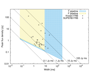
Figure 1: Left: Single-pulse search sensitivity plot for the SUPERB survey. Over-plotted are the 27 known FRBs with the relevant parameters published, including the five SUPERB discoveries (see the FRB Catalogue of Petroff et al. 2016, Keane et al. 2016 and Paper 2 for more details). Right: Periodicity search sensitivity plot for the SUPERB survey with the known pulsar population over-plotted in sub-groups (denoted by different symbols and colours) divided by their DM values.

The first SUPERB observing run was in April 2014 and lasted for 2 days. Subsequently it ran with some regularity from July 2014 to January 2016. January 2016 to late 2016 saw a hiatus as Parkes was used primarily to commission a phased-array-feed (Deng et al., 2017), but SUPERB resumed observations from December 2016. In this first paper we consider the results up to the end of January 2016. The major observing parameters are outlined in Table 1 and the motivations for these choices are given below. Additionally, the entire list of survey pointings performed to the end of January 2016, illustrated in Figure 2, is included in the additional online material associated with this article.

Table 1: Observational parameters of the survey. Where two values are given the first is for SUPERB (P858) and the second is for the SUPERBx (P892) components of the project.

Parameter	Value
Regions (P858)	$-120^{\circ}<l<50^{\circ}$, $15^{\circ}<|b|<25^{\circ}$
	$29^{\circ}<l<50^{\circ}$, $-25^{\circ}<b<25^{\circ}$
Regions (P892)	$-140^{\circ}<l<50^{\circ}$, $25^{\circ}<b<45^{\circ}$
	$-140^{\circ}<l<50^{\circ}$, $-30^{\circ}<b<-25^{\circ}$
	$-140^{\circ}<l<50^{\circ}$, $b<-45^{\circ}$
	$-140^{\circ}<l<-120^{\circ}$, $-25^{\circ}<b<25^{\circ}$
$\tau_{\rm obs}$ (s)	$\sim 560$
$N_{\rm beams}$ (planned)	86424 and 180583
$N_{\rm beams}$ (observed)	71572 and 141512
$T_{\rm samp}$ ($\upmu$s)	64
$\Delta\nu$ (MHz)	400
$\Delta\nu_{\rm chan}$ (kHz)	390.625
$N_{\rm chans}$	1024
$N_{\rm samples}$	$\sim$223
$N_{\rm bits}$ (online search)	2 (periodicity), 8 (single pulse)
$N_{\rm bits}$ (offline search)	2
$N_{\rm bits}$ (archival)	2
Archived data (TB)	154 and 303

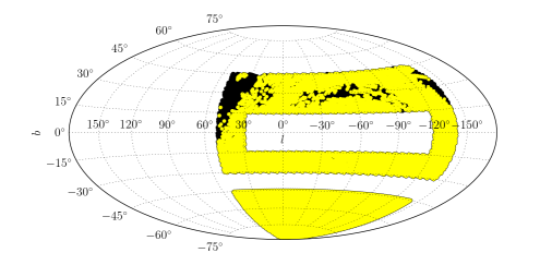
Figure 2: An Aitoff projection of the sky in Galactic coordinates. Those regions covered with 9-minute SUPERB pointings are marked in yellow. Pointings planned, but not yet observed before the end of January 2016 are marked in black.

3 Infrastructure

One of the core objectives of SUPERB is to enable real-time pulsar and FRB searches. Thus it requires comprehensive infrastructure with minimal human input to allow for automated operation. Below we describe the data acquisition, processing pipelines and data management scheme used in the project, which is shown schematically in Figure 3.

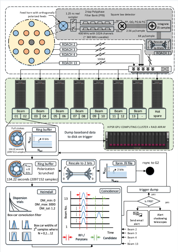
Figure 3: A schematic of the SUPERB acquisition and data analysis pipeline. The top most block shows the Parkes primary beam (yellow) with the 13-beam pattern of the multi-beam reciever over-plotted. Each beam is processed separately in the same way (grey block) on a Roach field programmable gate array — Nyquist sampled in two orthogonal polarisations, formed into a filterbank, square-law detected to polarisation products and integrated down in time, rescaled from 32 bits to 8, then transferred to a GPU-enabled computing cluster for further searching (green block). The F pipeline single-pulse search happens on these machines — a ring buffer in memory is searched for dispersed pulses satisfying several criteria (see main text) to identify these as FRB candidates. Bona fide FRB candidate information is sent to other telescopes for data dumps (for shadowing telescopes) and/or follow-up.

3.1 Data Acquisition

SUPERB makes use of a modified version of the observing system described by Keith et al. (2010). Here the Berkeley Parkes Swinburne Recorder (BPSR) backend is used to digitise, filterbank, detect and temporally average the signal from each beam of the Parkes 21-cm multibeam receiver (Staveley-Smith et al. 1996). The output from BPSR is an 8-bit, full-Stokes filterbank with 1024 frequency channels spanning 400 MHz of bandwidth (1182 - 1582 MHz) and 64-$\upmu$s time resolution. As noted by Keith et al. (2010) the effective bandwidth is $\sim$340 MHz due to the presence of strong RFI from communication satellites emitting in the 1525-1559 MHz band and roll-off at the band edges (see § 5.4). The output from BPSR is sent to the HI-Pulsar Signal Processor (HIPSR, Price et al. 2017) backend for further processing. It is here that the observing systems of HTRU-S and SUPERB diverge. Where previously data arriving in HIPSR would have been bit-compressed and the Stokes I component written to disk and thence to magnetic tape, for the SUPERB survey the data are instead pushed into a 120-s ring buffer. This ring buffer serves two purposes; it provides input to a real-time transient search and it enables full-Stokes data to be recorded upon receipt of a trigger. Following the transient search, the Stokes I component of the data is bit-compressed to 2 bits per sample and is written to disk on HIPSR. The removal of the magnetic tape storage step, employed by HTRU-S and previous surveys, is significant as the writing of data to tape had been the major contributing factor in discovery lag.

3.2 Processing Hardware

Upon completion of an observation at Parkes the data are streamed from the HIPSR backend to the Green II (G2) supercomputing cluster located at the Swinburne University of Technology. The G2 is composed of three main components, the SwinSTAR and gSTAR compute clusters and a $\sim$5 PB lustre file system. For the purposes of SUPERB data processing we are primarily interested in the number of GPUs available on each cluster, to wit SwinSTAR provides 47 nodes each with two six-core X5650 CPUs, 48 GB of RAM and two Nvidia Tesla C2070 GPUs and gSTAR provides 61 nodes each with two eight-core E5-2660 CPUs, 64 GB RAM and a Nvidia Tesla K10 GPU. SwinSTAR further provides 3 high-density nodes, each with two six-core X5650 CPUs, 48 GB RAM and seven Tesla M2090 GPUs. G2 uses a PBS-based queue system, employing Torque and Moab for resource management and job scheduling, respectively.

3.3 Processing Pipelines

Data observed as part of SUPERB are searched for both periodic and transient signals. In both cases the data go through both a fast (F) and thorough (T) version of the respective processing pipeline. The objective of the F pipeline processing is to enable real-time processing, picking up the brighter signals with less extreme properties, while the objective of the T pipeline processing is to maximise our chances of discovery by searching a larger volume of parameter space with higher resolution. Below we describe the F and T versions of both our periodicity and transient searches, which is shown schematically in Figure 4.

Figure 4: A schematic of the SUPERB processing pipelines on gSTAR.

3.3.1 Transient Search Pipeline

While the data are still stored in the 120-s ring buffer on the HIPSR system they are searched using the F pipeline for single pulses while still at 8-bit precision. This pipeline uses the heimdall software package to search 16-s segments (or ‘gulps’) of incoming data over a range of pulse widths, and dispersion measures for signals with properties resembling those of real astrophysical pulses. The F pipeline search is restricted to 1623 DM trials between 0 and 2000 pc cm^-3 and 13 width trials between $0.064$ and $262.144$ ms. The maximum DM was in December 2015, increased to 3000 pc cm^-3. The search is run on each beam individually to produce a list of candidates which are then cross-correlated between beams to eliminate local RFI which occurs uniformly, or in non-neighbouring beams. Frequency channels of known sources of RFI are masked during the search to limit contamination. Several cuts, described in the following section, are applied to the resulting candidates for each gulp to search for FRBs; the list of single-pulse candidates is not saved to disk.

After a pointing is completed the data are saved as filterbank files and sent to the gSTAR supercomputer at Swinburne, they are searched again for single pulses using the T pipeline. This pipeline is an expanded version of the F pipeline on HIPSR which searches an entire pointing over a larger parameter space to ensure that no viable candidates are missed. For the T pipeline the pointing is searched up to a maximum DM of 10,000 pc cm^-3 using 1986 DM trials, and searched for pulses up to a maximum width of $262.144$ ms. The beams are processed in a similar manner to the F pipeline, i.e. individually and then compared to remove coincident RFI. Additional RFI excision occurs in the form of frequency masking (as with the F pipeline) and an eigenvector decomposition based algorithm (Kocz et al., 2010). The list of single-pulse candidates are, in this case, saved to disk.

Table 2: The processing parameters for the F and T transient and periodicity search pipelines.

Single-pulse pipeline parameter	F pipeline	T pipeline
DM range (pc cm-3)	0–2000	0–9988
DM trials, $N_{\rm DM}$	1623	1986
Width trials	$(1-2^{12})\times t_{\mathrm{samp}}$	$(1-2^{12})\times t_{\mathrm{samp}}$
RFI excision methods	Bad channels	Bad channels
		eigenvector excision
Periodicity search pipeline parameter	F pipeline	T pipeline
Maximum DM, $\rm{DM}_{\rm max}$ (pc cm-3)	400	400
Trial DMs, $N_{\rm DM}$	884	1448
Maximum acceleration, $|a_{\rm max}|$ (m s-2)	25	250
Acceleration trials, $N_{\rm acc}$	36	549
Number of harmonic folds performed, $N_{\mathrm{h}}$	4	4
RFI excision methods	Bad channels	Bad channels
	Birdie list	Birdie list
		Eigenvector excision

3.3.2 Transient Candidate Selection

After running the F and T pipelines the above parameters produce a sizeable number of candidates. These are parsed according to the following rules. In the F pipeline we apply:

$$\mathrm{DM}\geq 1.5\times\mathrm{DM}_{\mathrm{Galaxy}}$$

$$\mathrm{S/N}\geq 10$$

$$N_{\mathrm{beams,adj}}\leq 4$$

$$W\leq 8.192\>\mathrm{ms}$$

$$N_{\mathrm{events}}(t_{\mathrm{obs}}-2\>\mathrm{s}\to t_{\mathrm{obs}}+2\>\mathrm{s})\leq 5$$ (1)

where DM and DM_Galaxy are the dispersion measure of the candidate and the modeled DM contribution from the Milky Way from the NE2001 model (Cordes & Lazio, 2002), respectively, S/N is the signal-to-noise ratio of the candidate, $N_{\mathrm{beams,adj}}$ is the number of adjacent beams in which the candidate appears, $W$ is the width of the candidate pulse, and the final cut describes the number of candidates detected within a 4-second window centred on the time of the candidate. If there are too many candidates in a time region around the candidate of interest it is ignored, a precaution to reduce the number of false positives due to RFI. The F pipeline only searches for pulses from FRBs, hence the high-DM cutoff for viable candidates. The excess DM factor of $1.5$ is arbitrary and might conceivably result in missed FRBs in the F pipeline (or initial classification of an FRB as a RRAT, see Keane 2016).

In the T pipeline the data are searched for single pulses from pulsars as well as pulses from FRBs to ensure that no candidates are missed in the full processing of the data. For the T pipeline we apply:

$$\mathrm{DM}\geq 2\leavevmode\nobreak\ \mathrm{pc}\;\mathrm{cm}^{-3}$$

$$\mathrm{S/N}\geq 8$$

$$N_{\mathrm{beams}}\leq 4$$

$$W\leq 262.144\>\mathrm{ms}$$

where the parameters are as in Equation 1. The T pipeline processing is intended to detect lower S/N FRBs and single pulses from pulsars (see Figure 5).

Figure 5: A single-pulse search candidate plot for a single SUPERB pointing. The top three panels show a histogram of events as a function of DM, then a histogram as a function of S/N, and a scatter plot of the DM and S/N of each candidate. The bottom plot shows the candidates in time and DM; here the colour corresponds to the pulse width and the number is the beam in which the candidate was detected. All candidates above a S/N of 8 are plotted here. In this example several pulses are evident in beam 13 at a DM of approximately 10 pc cm^-3. We note that the bottom panel’s axis label is DM$+1\;\mathrm{pc}\;\mathrm{cm}^{-3}$ rather than simply DM. The reason for this is that a base-10 logarithmic scaling is appropriate for our DM sampling, but there is still a need to display zero DM events to identify RFI. RFI signals peak at zero DM and depending on their time duration can be detected at higher DM values also.

3.3.3 Periodicity Searching

Periodicity searching of the SUPERB survey is performed using the GPU-enabled pulsar searching code, peasoup. To implement a real-time pipeline, the three high-density gSTAR nodes (21 Tesla M2070 GPUs) were reserved for all SUPERB observing sessions. The search parameters are summarized in Table 2.

In both F and T pipelines, we fold all candidates detected by peasoup with a S/N higher than $9$, and always fold the $24$ brightest candidates of every beam. Figure 6 shows an example of candidate diagnostic plots from the periodicity search. Motivated by the difficult RFI environment at Parkes and the constraint of real-time processing for the F pipeline, a folding software package named cubr has been written for the survey. It can fold candidates in parallel, which reduces processing time by a factor of $\sim 5$ as compared to equivalent tools in the psrchive package (Hotan et al., 2004). It also has the ability to delete interference signals directly in the folded data; abnormal frequency channels or sub-integrations are identified using an outlier detection method and the corresponding data are replaced by an appropriately chosen constant value. This has the benefit of reducing the difficulty of candidate evaluation, and in some cases identify pulsars that would otherwise be entirely masked by interference (see Figure 7). cubr’s RFI mitigation algorithms are described in length in Morello (2016).

Figure 6: An example candidate plot from our pulsar searching pipeline: this is the first detection of PSR J1421$-$44. The panels shown are, in grey scale, the period-folded signal as a function of frequency (top) and time (bottom), a folded pulse profile (blue profile) and a curve showing the S/N as a function of DM. Pertinent information about the pointing and candidate are also displayed. Diagnostic plots such as these are often used in examining candidates arising from our pipelines.

Figure 7: An observation of PSR J1759$-$1029 ($P=2.512$ s) before and after the application of the cubr RFI mitigation algorithms. The pulsar’s signal is the vertical trail (two periods are shown for readability), and is demonstrably nulling in sub-integrations 20 to 25. Top left panel: a strong, periodic sine-wave like RFI is present in frequency band no. 10. Middle left panel: additionally, three bright dashes correspond to brief bursts of broadband interference; they are also visible in the sub-bands plot as curved trails, and generate secondary pulses in the overall folded profile (bottom panel). Right column: the same plots after the application of interference mitigation algorithms.

3.3.4 Periodicity Candidate Selection

The combined output rate of both periodicity search pipelines is approximately 4,000 candidates per observed hour, and they have generated a total of 5.9 million folded candidates so far. Visual inspection of all candidates is not a viable option considering the thousands of hours of tedium it would involve and more importantly the real-time discovery constraint we set for the F pipeline. We therefore entirely transferred the task of candidate selection to a Machine Learning algorithm. We use an improved version of the SPINN (the Straightforward Pulsar Identification Neural Network) pulsar candidate classifier (Morello et al., 2014). It is an artificial neural network that evaluates candidates based on eight numerical features, and outputs a score between 0 and 1 that can be interpreted as the likelihood of being a pulsar.

SPINN was trained on a large sample of candidates obtained by running our search and folding pipeline on the HTRU-S Intermediate Latitude survey (Keith et al., 2010), which was observed between 2008 and 2010 with the same telescope, instrument, and sampling and integration times, but covered an area of the sky that does not overlap with that of SUPERB. We could therefore rigorously test the classification accuracy of SPINN on a sample of SUPERB candidates, knowing that none of those could have been ‘seen’ by the algorithm during training. Using the ephemerides published in the ATNF pulsar catalogue (Manchester et al., 1990), we manually identified every known pulsar detection found by peasoup during the first part of the survey (up to April 2015). This gave us a test sample of 139 pulsar detections along with 1,418,598 non-pulsar candidates which were scored by our classifier. From there we computed classification error rates as a function of score selection threshold; the results are summarized in Figure 8.

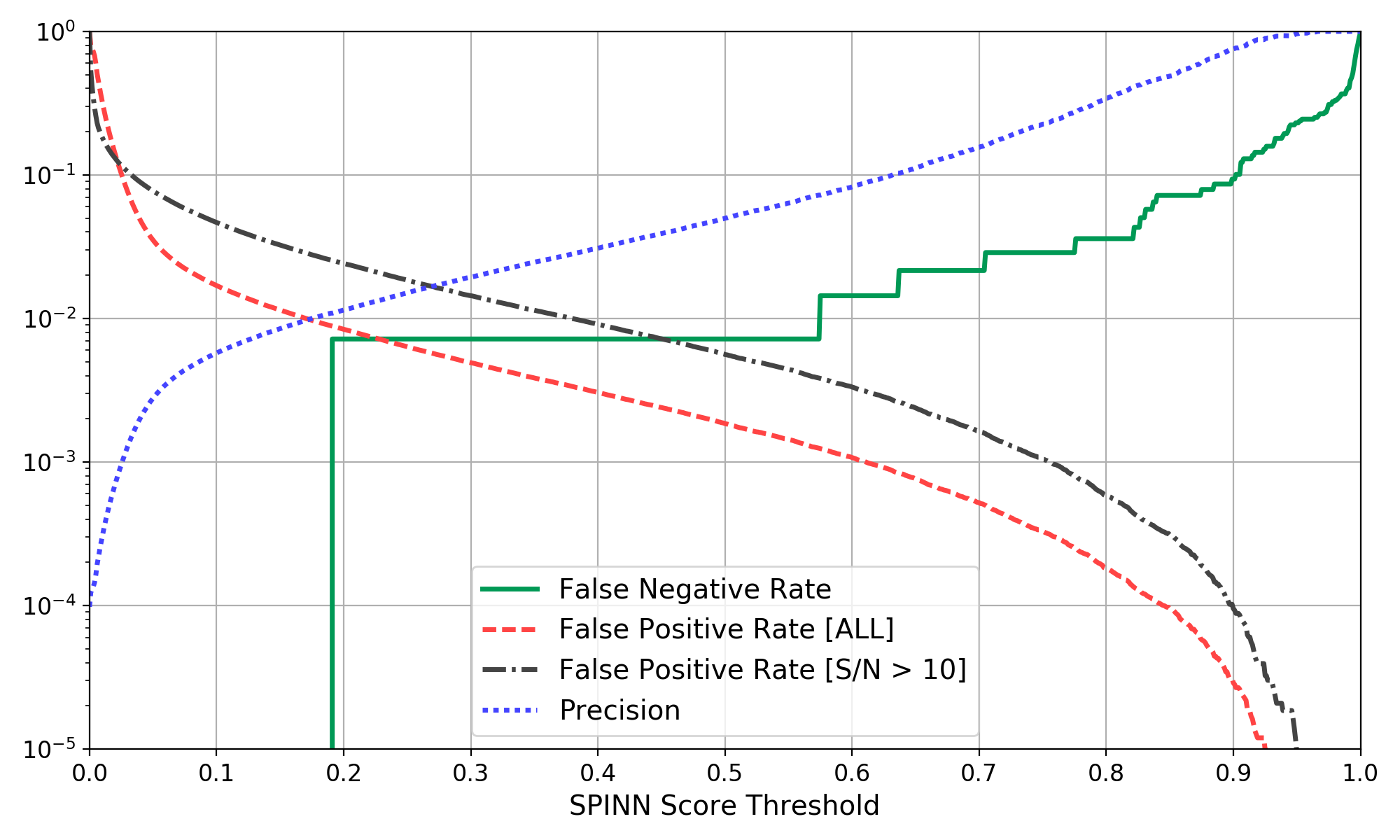
Figure 8: Classification error rates (log-scale) of SPINN as a function of output score selection threshold. The false negative rate is the fraction of pulsars missed (green line). The false positive rate is the fraction of spurious candidates incorrectly reported as pulsars (red line). We also evaluated it on the subset of candidates with $\mathrm{S/N}>10$ (black line), since those cannot be trivially rejected by the classifier based on their lack of statistical significance. Precision (blue line), is the fraction of genuine pulsars contained in the sample of candidates selected by the classifier, a relevant metric for the real-time detection pipeline.

We use different neural network score thresholds for the F and T pipeline. For real time discovery, we select candidates scoring higher than 0.85 to ensure a small false positive rate ($\approx$ 1 in 10,000) so that discovery alerts are reliable and can be acted upon quickly. In the T pipeline, we value search completeness most highly and therefore tolerate a higher false positive rate at the cost of a longer round of visual candidate inspection; we typically inspected candidates down to a score of 0.5, and 0.4 for millisecond pulsar candidates. This involved looking at on order of 10,000 candidate plots over the course of the entire survey.

3.3.5 Peryton Pipeline

At the inception of the project we planned to search for ‘perytons’ (Burke-Spolaor et al., 2011). These transient signals had been detected in archival data from Parkes with more than a decade of discovery lag and, although clearly terrestrial in nature, their source had yet to be pinpointed as of 2014 when SUPERB was beginning. We searched for perytons as for transient events above but with two slight modifications. Firstly, to take advantange of the fact that perytons are local and therefore detectable in most or all 13 beams of the receiver, the 13 beams are added to produce a new filterbank. Astrophysical events, which are typically in a single beam, are thus suppressed in S/N by a factor of $\sqrt{13}\sim 3.6$ whereas peryton signals are boosted by up to this factor in the resultant data set. This data is then searched as per the single-pulse search of a single beam. In identifying peryton candidates the number-of-beams sifting rule does not apply, and no DM cut is applied. SUPERB thus has the ability to discover peryton events in real time and did this when they first occurred during SUPERB observations in January 2015. The combination of the ability to identify these signals without any discovery lag, and the data from the RFI monitor installed at Parkes in December 2014 allowed the source of the perytons to be identified. The simultaneous coverage up to 3 GHz allowed us to identify the carrier frequency of $\sim 2.4-2.5$ GHz and through a process of deduction the culprit: unshielded microwave ovens on site. This work is discussed in more detail in Petroff et al. (2015). Since this time a live peryton search is not routinely performed but the publicly available survey data still contains these signals should others wish to pursue this study.

3.3.6 Future Pipelines

(i) Fast Folding Search: Due to short observing lengths the survey suffers a sensitivity loss to long-period pulsars that cannot be detected through their single pulses. It has long been known that the Fast Folding Algorithm (FFA, Staelin 1969) offers the possibility to recover sensitivity to these pulsars, even in short and noisy observations. Due to its computationally intensive nature, the FFA has seen only sparse use in blind pulsar surveys to date (although it has seen use in targeted searches, see e.g. Kondratiev et al., 2009). However, renewed interest in FFAs (Cameron et al., 2017) and their implementation on many-core compute architectures has led to the development of new codes that can be applied to the SUPERB data set. The application of an FFA to SUPERB data will address known biases in our processing and greatly improve our capability to discover pulsars at the long-period extreme of the population. This pipeline commenced in April 2017 and the results of this will be reported at a later date.

(ii) Low-Level RFI Mitigation Algorithms: In both the transient and periodicity search pipelines, most of the burden of RFI rejection is currently placed on the final candidate selection stage. This approach is not optimal since interference occurring during a pulsar observation can be strong enough to make the pulsar’s signal completely unrecognizable at the candidate inspection stage, even by a highly trained expert. In particular, a very common and unwelcome occurrence in SUPERB data is that of bright, broadband non-dispersed pulses lasting several milliseconds that are simultaneously visible in all beams of the receiver. These negatively impact the detectability of slow pulsars in the Fourier domain and are a prolific source of false positives to the single-pulse search. Existing tools such as the rfifind routine of the presto package (Ransom et al., 2002) do not effectively mitigate their effects. An attractive approach here is the application of spatial filtering (Leshem & van der Veen, 2000; Raza & van der Veen, 2002; Kocz et al., 2010), which is particularly efficient at identifying and canceling any interfering signal present in a large number of beams; while normally applied to baseband data, we are currently investigating the use of spatial filtering on incoherent filterbanks, allowing its deployment on archival data.

4 Multi-wavelength Synergies

The Parkes telescope is the primary instrument of the SUPERB project. However it is joined in its search efforts for varying amounts of time by a number of additional facilities, some of which work simultaneously and some of which react to triggers from Parkes. In this section we describe the shadowing (simultaneous observations) and triggering performed in the electromagnetic spectrum as well as multi-messenger searches for counterparts to Parkes discoveries.

4.1 Shadowing

The observations at Parkes are shadowed to various degrees by other telescopes. At the time of writing, this has been done with the upgraded Molonglo Synthesis Telescope (UTMOST), the Giant Metrewave Radio Telescope (GMRT) and the Murchison Widefield Array (MWA). At the conception of the SUPERB project in late 2013 the intention was to shadow Parkes with Molonglo at all times. By the start of the first SUPERB observing session in April 2014 the shadowing infrastructure was in place, but the Molonglo upgrade, was still in progress. Upon detection of an FRB a ring buffer of the polarisation power data at Parkes is dumped and a signal is sent to Molonglo to dump the single polarisation complex voltage data from every module in the array. The idea is to detect the signal at both telescopes and, in the case of an FRB localise the signal an order of magnitude more precisely than either telescope can do by itself and to obtain vital information on spectra. This concept is illustrated in Figure 9.

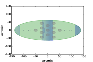
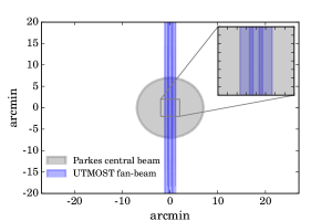
Figure 9: The left-hand panel shows a Molonglo primary beam (green) at 843 MHz over-laid on the 13-beam sky footprint of Parkes (grey). Some Molonglo fan-beams are also shown. A simultaneous detection at both telescopes can thus be used for more precise localisation than can be achieved at either telescope operating by itself. The right-hand panel shows a zoom-in on a single Parkes beam and shows three overlapping Molonglo fan-beams. Parkes FRBs are typically (although not always) in a single beam; Molonglo FRB detections are typically in 1 to 3 fan-beams. Combining this information an FRB can be localised an order of magnitude more precisely than with Parkes alone.

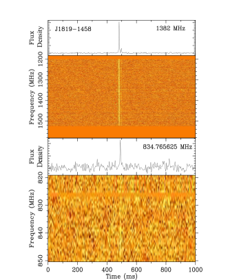
Figure 10: First simultaneous detection of a pulse from J1819$-$1458 at Parkes and Molonglo. The top panel shows the detection at Parkes, and the bottom the simultaneous detection at Molonglo. Note the different vertical scales for frequency.

Tests of this joint observing mode were performed using the erratic pulsar J1819$-$1458 (McLaughlin et al., 2006) which has a known spectrum and exhibits very bright pulses every $\sim$minute at 1.4 GHz at Parkes. The initial tests revealed that the sensitivity of Molonglo was less than $1\%$ of its final target sensitivity and as such Molonglo shadowing, though available, was not utilised for most of the observations reported here. However in the interim the Molonglo upgrade has proceeded at pace, further tests with J1819$-$1458 were a resounding success (see Figure 10), and the sensitivity is now at a level above $10\%$ of the theoretical optimum. This progress is well illustrated by the recent independent discoveries (i.e. not in tandem with Parkes) of 3 FRBs by UTMOST (Caleb et al., 2017).

The MWA ($\sim 600$ ${\rm deg}^{2}$ field of view at $200$ MHz) is also used, on occasion, to shadow SUPERB. Occasional shadowing has been performed since mid-2015 with more routine shadowing since January 2016. Data are recorded using the standard mode of the MWA’s hybrid correlator, recording visibilities at a cadence of 500 ms and 40 kHz. Furthermore, since the MWA’s sensitivity is a strong function of zenith angle, in order to keep the loss in sensitivity minimal and ensure quality calibration, Parkes pointings that are west-most are preferentially selected while the MWA is available for shadowing (but see § 5.4 for discussion of the RFI implications of this). The large field of view means there are no addition requirements in terms of additional calibration observations as multiple suitable sources are typically present for any given MWA pointing.

The 30-antenna GMRT is also used, on occasion, to shadow SUPERB, in particular in the 325-MHz band, where the 84^′ (FWHM) beam is well-matched to Parkes as it fully encompasses all 13 beams of the multi-beam receiver, albeit with non-uniform sensitivity. Simultaneously detecting a potential low-frequency counterpart allows one to constrain both the spectral nature and scattering properties of any FRBs in addition to the ability to precisely localise it in the sky (at the level of a few arcseconds). Shadowing with GMRT is complex as one must consider the down time due to the difference in slew rates, the need for approximately hourly phase calibration observations. Data are recorded using the high-time resolution mode of the GMRT software correlator (Roy et al., 2010) whereby the visibilities are recorded once every 125 ms, at a spectral resolution of 65 kHz, over a bandwidth of 16.66 MHz, centred at a frequency of 325.83 MHz. Despite the inevitable temporal and dispersive smearing expected for any potential counterparts to the FRB signals, this still ensures good detection prospects; e.g. a putative low frequency counterpart of FRB 110220 would be detectable as a 7$\sigma$ event. The time allocation and coordination considerations typically allow shadowing about 10% of the SUPERB survey. The common visibility is ensured by preferentially going for Northerly pointings ($\delta>-40^{\circ}$) that are past transit for Parkes during the times the GMRT is used (again see § 5.4).

4.2 Triggering

When an FRB is found in the F Pipeline burst search an alert is issued to the observers via email which can be visually inspected and assessed. If the signal is judged to be a FRB detection, a trigger is issued to collaborators for multi-wavelength follow-up. SUPERB maintains agreements with a large number of telescopes and collaborations to search for the signatures of FRBs across the electromagnetic spectrum. At the highest energies, SUPERB triggers the High Energy Spectroscopic System (HESS, Bernlöhr et al. 2003) operating in the range 10 GeV – 10 TeV. At X-ray wavelengths the Swift satellite (Burrows et al., 2005) is triggered, which then observes X-ray photons from $0.2-10$ keV.

Additionally, triggers are sent to the 2-m Liverpool telescope in La Palma, the 1.35-m Skymapper telescope in New South Wales, Australia, the 1-m Zadko telescope in Western Australia, the 2.4-m Thai telescope, the 8.2-m Subaru telescope in Hawaii and the 10-m Keck telescopes in Hawaii, the 6.5-m Magellan telescopes in Chile, and the Blanco 4-m telescope in Chile using the Dark Energy Camera (DECam). At radio wavelengths, triggers are sent to the 64-m Sardinia radio telescope capable of observing at 1.4 GHz, the GMRT, and the MWA (Tingay et al., 2013). Internally, the SUPERB collaboration also operates the Australia Telescope Compact Array (ATCA) to image the field of the FRB at 5.5 and 7.5 GHz. Follow-up timing of pulsar discoveries is also performed by some of the radio telescopes in this network.

Table 3: The network of instruments alerted to SUPERB FRB triggers.

Telescope name	Band/filters
H.E.S.S.	10 GeV – 10 TeV
Swift	0.2 – 10 keV
Liverpool Telescope	$R$
Skymapper Telescope	Hα, $ugvriz$
Zadko Telescope	$R$
Thai National Observatory	$R$
Blanco Telescope	$ir$VR
Subaru Telescope	$r^{\prime}i^{\prime}$
Keck Telescope	$400-1100$ nm
Magellan Telescope	J
MWA	185 MHz
GMRT	1.4 GHz, 610 MHz
Sardinia Radio Telescope	1.4 GHz
Effelsberg	1.4 GHz
ATCA	$4-8$ GHz

4.3 Multi-messenger Searches

The SUPERB project has agreements in place with multi-messenger facilities to search for counterparts to FRB events. A subset of FRB progenitor models involve merger events of compact objects and as such may have an associated gravitational wave counterpart. Furthermore the redshift ranges for many of the FRBs are plausibly within the relevant redshift horizon for ground-based gravitational wave detectors. As such we have an agreement in place with the LIGO consortium to identify counterparts in the Advanced LIGO dataset. Some FRB progenitors may also exhibit a neutrino signal. Earth-based neutrino detectors, which are sensitive to muon interactions with neutrinos, use the Earth itself as a filter against background muon signals, essentially look through the planet. We have an agreement with the ANTARES collaboration (Ageron et al., 2011) to search for neutrino signals associated with FRBs.

4.4 Public Alerts

From 2018-04-01 SUPERB will issue public alerts of FRB discoveries, with an associated Astronomer’s Telegram. The alert will be in the VOEvent Standard in the FRB format currently being finalised. While at present Parkes is the dominant FRB search machine, having discovered $22$ of the $31$ FRBs known, it is envisioned that other instruments, in particular CHIME, ASKAP and MeerKAT, will soon contribute significantly to the known population. As such it makes sense to create and adopt a world standard for FRB followups, and it is widely considered that public alerts are the best way to do this. The lead time to change to public alerts, as opposed to immediate adoption, is (a) to allow us to satisfy our commitments under agreements with partner instruments; and (b) allow finalisation of the format for FRB VOEvents and development of associated tools, which is currently underway.

5 Results

In this section we describe the first results from the survey, including verification of the expected sensitivity, the impact of radio frequency interference on the survey, and discoveries of FRBs and pulsars.

5.1 Survey Sensitivity Verification

To verify that the expected sensitivity of the survey is being achieved we keep track of all of the detections of previously known pulsars, detected in the pipelines described above.

Single-pulse search: The sensitivity of the SUPERB survey to single pulses from pulsars was compared to the sensitivity from the HTRU survey (Burke-Spolaor et al., 2011) for a subset of the detected pulsars. The theoretical flux denity of a single pulse detected by the multi-beam receiver is given by the modified radiometer equation:

$$S_{\mathrm{peak}}=\frac{(\mathrm{S/N})T_{\mathrm{sys}}\beta}{G\sqrt{n_{\mathrm{p}}\,\Delta\nu\,W}}$$ (3)

where $S_{\mathrm{peak}}$ is the peak flux density of the pulse, S/N is the signal-to-noise ratio as before, $\beta$ is a correction factor to account for small loses due to the digitisation ($\beta\approx 1.066$ for 2-bit digitisation in our case), $G$ is the gain of the telescope beam, $n_{\mathrm{p}}$ is the number of polarisations summed to create the signal, $\Delta\nu$ is the bandwidth, and $W$ is the pulse width. For a single pulse detected in the primary beam of the receiver with a S/N of 10 and a width of 1 ms this corresponds to a peak flux density of 0.5 Jy. The sensitivity to single pulses was found to be unchanged between the SUPERB and HTRU surveys and consistent with flux densities expected from Equation 3.

Periodicity search: We directly folded the survey data (up to and including February 2015) using ephemerides of all known pulsars that had a published mean flux density, $S_{\mathrm{mean}}$, at 1400 MHz and whose position was observed at least once. After visually inspecting the output we identified 124 detections of such pulsars and recorded their S/N. Using the modified radiometer equation appropriate for folded observations one can compute the expected folded S/N of a pulsar with duty cycle $\delta$:

$$\mathrm{S/N}=\frac{gS_{\mathrm{mean}}G\sqrt{n_{\mathrm{p}}\,\Delta\nu\,T_{\mathrm{obs}}}}{\beta T_{\mathrm{sys}}}\sqrt{\frac{1-\delta}{\delta}}$$ (4)

where $T_{\mathrm{obs}}$ is the integration time, and $g=\exp(-\alpha^{2}/2\alpha_{0}^{2})$ is an adjustment to the boresight gain due to positional offset of the pulsar — the beam response is Gaussian; $\alpha_{0}=6.0$ arcmin for the Parkes multi-beam receiver. Figure 11 displays the measured vs. expected folded S/N for our sample of pulsars. The vast majority of sources follow the identity line as it should be. The only notable exception is PSR J0904$-$7459: it was seen twice with a S/N approximately 30 times lower than expected, and failed to be detected in two other observations where it should have been seen with S/N $\approx$ 150. These repeated and consistent discrepancies suggest that the catalogued flux density of B0904$-$74 (J0904$-$7459) is erroneously high, an inference which is supported by a recent large scale study of pulsar spectral properties (Jankowski et al., 2017). As a result of this realisation the pulsar catalogue (version 1.56) has now been updated to reflect our observations (R.N. Manchester, priv. comm.).

We also checked which known pulsars of our sample were not properly detected by our search pipeline. The notable non-detections of peasoup are listed in Table 4. None of those are surprising as they can be explained by either the presence of RFI, or the fact that the FFT tends to lose sensitivity to signals with long periods. SPINN gave a score lower than 0.5 only to a single pulsar observation, whose candidate plot was heavily affected by impulsive RFI. This can also be seen in Figure 8, where the false negative rate at a score of 0.5 is not quite zero.

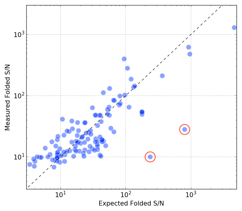
Figure 11: Measured versus expected folded S/N for known pulsars whose position was observed during the first part of the survey (excludes SUPERBx). The dashed line materializes the expected 1:1 correlation. Expected S/N has been computed under the assumption of a 5% pulsar duty cycle. The outliers circled in orange correspond to two detections of J0904$-$7459, whose previously catalogued flux density at 1400 MHz appears to have been vastly larger than what our data indicates (see text).

Table 4: List of notable non-detections of peasoup. We also ran the seek routine of the well-established sigproc pulsar searching package, and obtained three faint detections. No major discrepancy can be seen though. One can also note the potential benefits of an FFA-based pulsar search. Note that J1910$+$0714 was affected by impulsive RFI, and J1105$-$4357 was impacted by the presence of periodic RFI at a period of 1000.0 ms.

Name	P (ms)	DM	Folded S/N	seek S/N
J1105$-$4357	351.1	38.3	12.2	6.9
J1842$+$0257	3088.3	148.1	13.9	6.7
J0633$-$2015	3253.2	90.7	14.0	$-$
J0636$-$4549	1984.6	26.3	14.0	$-$
J1846$-$7403	4878.8	97.0	14.1	6.4
J1910$+$0714	2712.4	124.1	17.6	$-$
J1945$-$0040	1045.6	59.7	24.6	$-$

5.2 FRBs

The first FRB discovered by SUPERB is FRB 150418. This source has been reported in Keane et al. (2016) and further discussed in many susequent publications as we now recap. FRB 150418 is at low Galactic latitude ($b=-3.3\degree$) but despite this is clearly extragalactic with $\mathrm{DM}/\mathrm{DM}_{\mathrm{Milky\;Way}}$ of $4.2$ ($2.4$) according to the NE2001 (YMW16) model of the electron density in the Galaxy (Cordes & Lazio, 2002; Yao et al., 2017). In brief the main point of subsequent discussion has been the statistical association (and its implications) discussed in Keane et al. (2016). This association, with a source in the elliptical galaxy WISE J071634.59$-$190039.2, was based on its contemporaneous brightening and an estimate of the likelihood of its light curve ($\sim 99\%$ probability of association, based on 5 observation epochs). Further observations at the highest angular resolutions show that the source (which must be more compact than $\sim 10$ pc) is most likely an AGN (Bassa et al., 2016; Giroletti et al., 2016). As more data became available the light curve of the variable radio source became ever better characterised and the statistical significance of the association reduced (to $\sim 92\%$, based on 24 epochs, see e.g. Williams & Berger 2016; Johnston et al. 2017). Unless a repeat FRB is seen from the source this association is thus likely to remain somewhat controversial, at least until such time as the statistics of longer ($\sim$day) timescale variability at below $100$ $\mathrm{\upmu Jy}$ becomes clearer.

Four further FRB discoveries from SUPERB will be reported in detail, along with their multi-wavelength and multi-messenger followup, in Paper 2 in this series.

5.3 New Pulsars

The first 10 pulsars discovered in this survey are listed in Table 5. For seven of these the positions listed denote the phase centre of the beam in which they were discovered and should only be taken as indicative prior to a full timing solution being obtained; the exceptions are identified below. Figure 12 shows the pulse profiles.

Table 5: The parameters of 10 newly-discovered pulsars from the SUPERB Survey. The timing solution for PSR J1421$-$4409 is detailed in Table 6. We list the positions in both Equatorial coordinates with uncertainties, and the equivalent Galactic coordinates omitting those same uncertainties, the spin period ($P$), the DM and the NE2001-derived distances of these pulsars. Values in parentheses are the nominal 1-$\sigma$ uncertainties in the last digits. We understand that two of these pulsars have been independently identified, but not yet published, in two other ongoing surveys denoted here as: * = GBNCC, ** = PALFA.

PSR name	R.A. (J2000)	Dec. (J2000)	$l$	$b$	$P$	DM	Dist	Comment
	(h:m:s)	$(^{\circ}:\,^{\prime}:\,^{\prime\prime})$	$(^{\circ})$	$(^{\circ})$	(ms)	(cm-3pc)	(kpc)
J0621$-$55	06:20.7(5)	$-$56:05(7)	264.822	$-$26.416	-	22	1.1	RRAT
J0749$-$68	07:50:50(1)	$-$68:44:27(4)	281.013	$-$20.110	915.171299(2)	26	1.1	scintillates
J1126$-$38*	11:26.3(5)	$-$38:38(7)	285.230	21.286	887.55(1)	46	1.7
J1306$-$40	13:06:56.0(5)	$-$40:35:23(7)	306.108	22.186	2.20453(2)	35	1.2	MSP, intermittent
J1337$-$44	13:37.1(5)	$-$44:43(7)	311.412	17.386	1257.52(9)	96	3.5	nuller
J1405$-$42	14:05.8(5)	$-$42:33(7)	317.249	18.233	2346.80(4)	64	2.0	-
J1421$-$4409	14:21:20.9646(3)	$-$44:09:04.541(4)	319.497	15.809	6.38572883816(3)	54.6	1.6	MSP, binary
J1604$-$31	16:04.4(5)	$-$31:39(7)	344.118	15.380	883.883(5)	63	1.9	-
J1914$+$08**	19:14.3(5)	$-$08:45(7)	43.327	$-$1.042	440.048(2)	285	7.0	-
J2154$-$28	21:54.8(5)	$-$28:08(7)	20.854	$-$51.089	1343.35(2)	28	1.2	-

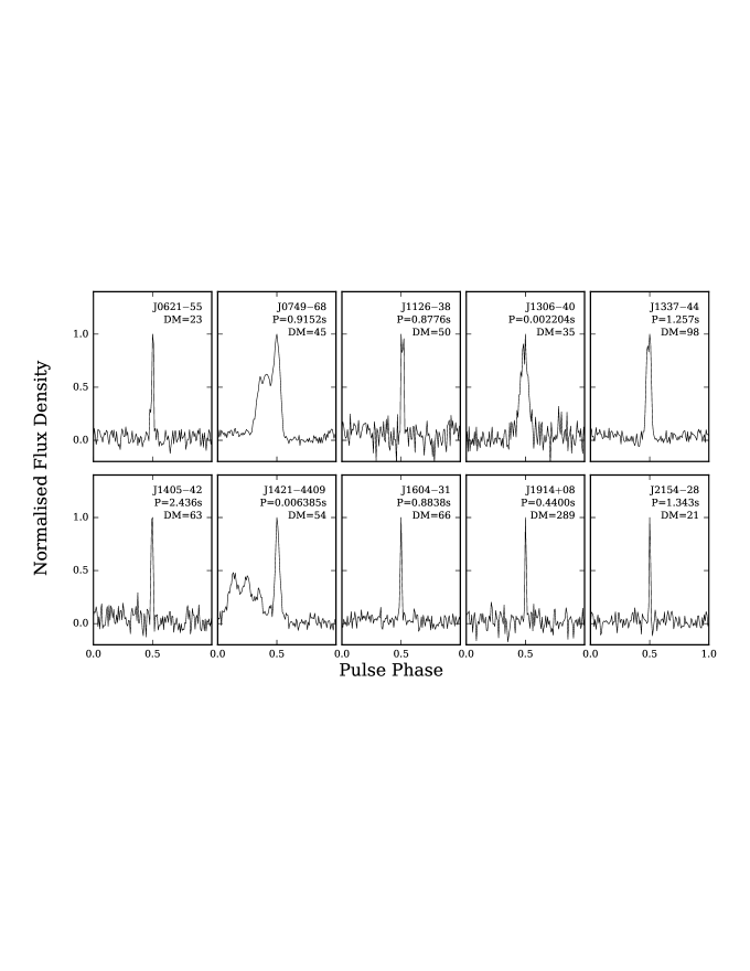
Figure 12: Pulse profiles of the first 10 pulsar discoveries from SUPERB. Each panel shows one pulse period and the pulsar name is given in the top right corner, along with its rotation period in seconds and dispersion measure in units of $\mathrm{cm}^{-3}\,\mathrm{pc}$. J0621$-$55 does not yet have a determined periodicity.

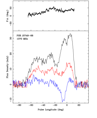
Figure 13: Polarisation properties of PSR J0749$-$68. In the upper panel the polarisation position angle is shown. In the lower panel black, blue and red denote total intensity, linear and circular polarisation respectively.

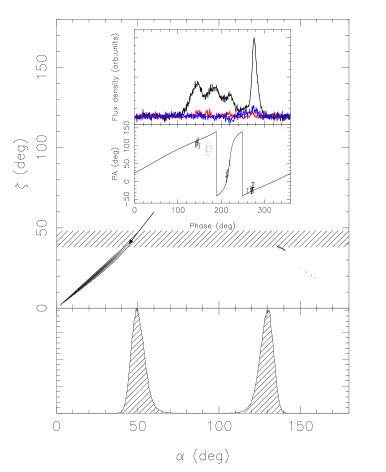
Figure 14: Polarisation properties of PSR J1421$-$4409. The main top panel shows the system geometry as derived from a least-squares-fit of the RVM to the PA of the linearly polarized emission; also shown are regions of the magnetic inclination angle ($\alpha$) and viewing angle ($\zeta$) plane with the best RVM fits (1-$\sigma$ contours). We also mark the constraint on the orbital inclination angle as a horizontal strip. Also, assuming a filled emission beam, we derive a distribution of inclination angles (lower panel) that is consistent with the observed pulse width. For the point that satisfies the profile, polarimetric and orbital inclination constraints ($\alpha\,=\,44^{\circ}$ and $\zeta\,=\,40^{\circ}$) we calculate the RVM PA versus phase curve and superimpose it on the measurements (bottom panel of inset). The top inset panel shows the pulse profile using the same conventions as in Figure 13.

PSR J0621$-$55: This source was found in the single-pulse pipeline and is undetectable in our periodicity searches. As such it can be classified as a ‘RRAT’ (Keane & McLaughlin, 2011). As only 3 pulses have been detected for this source it has not yet been possible to identify any underlying periodicity.

PSR J0749$-$68: This pulsar is undetected in several observations but has high S/N in others; its period averaged flux density is $4.1$ mJy. This may be due to scintillation or possibly nulling. The profile is broad with a width of $80\degree$. It has a 40% linear polarization fraction which is high given the pulsar’s long spin period. Circular polarization is modest and shows a change in sign close to the profile peak (see Figure 13). We measure the rotation measure to be $-23\pm 2\;\mathrm{rad}\,\mathrm{m}^{-2}$. The position angle swing is relatively flat leading to the conclusion that the pulsar is an almost aligned rotator. A partial timing solution has been obtained for this pulsar so that, as indicated in Table 5, its position is determined more accurately than most of the sources presented here.

PSR J1126$-$38: This 887-ms pulsar, although not previously reported, appears to have also been independently discovered by the Green Bank North Celestial Cap (GBNCC) survey.

PSR J1337$-$44: This slow pulsar appears to be nulling and as such is difficult to time, at least at $\sim 1.4$ GHz. Our efforts to observe this source at $\sim 750$ MHz at Parkes (pulsars generally being stronger at these lower frequencies, Bates et al. 2013) have been scuppered due to the recent appearance of strong terrestrial RFI in the band. The origin of this RFI is a 4G telephone base station now located less than $10$ km from the telescope. Given this and the Southerly declination of the source it may evade a full timing solution for a while. The nulling seems to be intrinsic as scintillation might be precluded as the pulsar’s DM implies a scintillation bandwidth that is much smaller than our observing bandwidth.

PSR J1405$-$42: This 2.3-s pulsar is the slowest in our sample. It would have been missed were it not for our RFI mitigation techniques. We expect our final pulsar sample to contain a much higher fraction of such slow pulsars as we focus efforts on relevant RFI mitigation strategies as well as optimised searching, e.g. with the FFA pipeline.

PSR J1604$-$31: In contrast to PSR J0749$-$68, the profile is very narrow with a width of only $5\degr$. The fractional polarization is low and no RM is measurable.

PSR J1914$+$08: This 440-ms pulsar is the one with by far the highest DM in our sample, as one might expect for the source that is closest to the Galactic plane. Although not previously reported, appears to have also been independently discovered by the Pulsar Arecibo L-band Feed Array (PALFA) survey.

PSR J2154$-$28: This pulsar was initially missed in the F pipeline but was detected in the T pipeline as a result of the additional RFI mitigation performed therein.

5.3.1 PSR J1306$-$40

This pulsar has a period of $2.2$ ms and has proven to be the most elusive of those reported here. It was initially detected in June 2015 in two survey pointings separated by 30 minutes (see Figure 15). The S/N of these initial two detections were $\sim 14$ and $\sim 23$. The source then proved undetectable in extended efforts to re-detect it in a total observation time of $9$ hours. Combining the two detections we derived an improved sky position for the source ‘in between’ the two survey pointings, by considering the beam model and weighting appropriately by the S/N values. Focusing on this refined position, our best estimate for the true position, we later re-detected the source twice again in September 2016 in observations 5 days apart. In each detection the signal is seen with a positive orbital acceleration where the convention is such that this implies we are observing the pulsar on the ‘near’ side of its orbit. Although four detections is a small sample this is suggestive of an ecclipsing system where the pulsar is not detectable when on the ‘far’ side of the orbit. The difficulty in detecting this source is also likely compounded by scintillation. The nominal sky position of the pulsar also happens to be within the field where there are $130$ ks of observation accumulated, by XMM Newton, as part of a study of a nearby Seyfert galaxy. In these data it can be seen that the nominal position of the pulsar is coincident with the source 3XMM J130656.2$-$403523. The spectrum of the source is at first glance consistent with what one might see in an ecclipsing ‘red back’ binary system, with a hint of variability on a $\sim 1/2$-day time scale, but it is unclear if the spectrum is reliable given the source’s location so close to the edge of the detector.

Linares (2017) has further studied these X-ray data, along with optical data from the Catalina Sky Survey, and derives a period of $26.3$ hr. Extrapolating this period to the times at which our radio detections have been made shows that our detections are indeed all on the ‘near’ side of the orbit, but with several non-detections also falling in this range. These non-detections might be attributable to scintillation or ‘transitional’ behaviour in the system. Overall the picture is consistent with the red back hypothesis. We will report in further detail on our ongoing studies of this source in future publications.

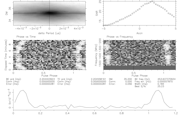
Figure 15: One of the detections of PSR J1306$-$40. The top-left panel shows the S/N (in grey scale) as a function of trial DM and period; the top-right panel shows S/N as a function of trial acceleration — a highly significant orbital acceleration is evident. The middle panels the S/N (grey scale) as a function of time during the observation (left) and frequency across the observing band (right). The bottom panel shows the integrated pulse profile at the optimised period, acceleration and DM.

5.3.2 PSR J1421$-$4409

Discovered in the real-time periodicity search pipeline, PSR J1421$-$4409 (hereon J1421) is the first millisecond pulsar discovered by SUPERB. Its pulse profile is complex as seen in many MSPs eg. Dai et al (2015) with half-maximum width of just $11.2\degree$ but, because of the trailing peak, reaches the 10 percent level only after $176\degree$ of pulse phase. The pulse averaged flux density is $1.4$ mJy and the linear polarization is low, at just $10\%$ (see Fig 14). We estimate the rotation measure to be $-43\pm 8\leavevmode\nobreak\ \mathrm{rad}\,\mathrm{m}^{2}$. The linear polarization loosely tracks the total intensity profile but the circularly polarized component becomes significant in the trailing half of the profile, presenting a change in handedness from right to left. Individual observations were polarization calibrated following the Measurement Equation Template Matching technique described in van Straten (2013) to correct for the cross-coupling of the feeds, using long-track observations of PSR J0437$-$4715. Additionally, the gain imbalance between the receiver feeds was corrected by utilising square wave observations of a noise diode with known polarization properties.

The pulsar has a 6.3-ms spin period and resides in a 30.7-day binary system. With a minimum companion of mass of 0.18 $M_{\odot}$, J1421 would appear to be a typical PSR-HeWD binary. However, binary periods of between 22 and 48 days are rare for MSPs (the “Camilo gap”; Camilo, 1995) with the only Galactic-field PSR-HeWD binaries known to have orbital periods in this range being the so-called eccentric MSPs (eMSPs, Barr et al. 2017). Although several have been proposed, there is currently no generally accepted model describing the evolution of eMSPs. One model of note for discussion of J1421 is that of Antoniadis (2014). In this model, hydrogen shell flashes at the end of the recycling phase result in a super-Eddington mass transfer rate between the donor and companion. Matter then cannot be accreted onto the neutron star and forms a circum-binary disk and it is through interaction with this disk that eccentricity is induced in the system. Antoniadis (2014) predicts that non-eccentric binaries can also exist in this gap if they are capable of photo-evaporating their circumbinary disks before they can induce eccentricity in the orbit. A pulsar’s capability to photo-evaporate its disk is proportional to its spin-down luminosity and inversely proportional to its semi-major axis distance. If we compare J1421’s properties to those of the eMSPs, we find that it has a slightly lower projected semi-major axis distance than the eMSPs (12.7 lt-s as compared to a median of 14 lt-s for the eMSPs) and its spin-down luminosity is close to the mean of the eMSPs, $4.6\times 10^{33}$ ergs s^-1. As such J1421 does not clearly distinguish itself from the eMSPs and thus presents a challenge to the circumbinary disk model.

Table 6: Ephemerides for PSR J1421$-$4409.

Parameter	Value (Error)
Epoch (MJD)	57600
Pulse period, $P$ (ms)	6.38572883816(3)
Period derivative, $\dot{P}$ (10-20)	1.27(4)
Right ascension, $\alpha$ (J2000.0)	14h21m20$\aas@@fstack{s}$9646(3)
Declination, $\delta$ (J2000.0)	$-$44°09′04$\aas@@fstack{\prime\prime}$541(4)
$\mu_{\alpha}$ (mas yr-1)	$-$10(8)
$\mu_{\delta}$ (mas yr-1)	3(2)
Composite proper motion, $\mu$ (mas yr-1)	11(8)
Celestial position angle, $\phi_{\mu}$ (°)	$-$70(2)
Dispersion measure, DM (pc cm-3)	54.635(4)
Binary model	ELL1
Solar System ephemeris	DE421
Orbital period, $P_{\rm b}$ (days)	30.7464535(2)
Projected semi-major axis, $x$ (lt-s)	12.706655(5)
Orbital eccentricity, $e$	0.0000128(4)
Epoch of periastron, $T_{0}$ (MJD)	56935.6(1)
Longitude of periastron, $\omega$ (°)	39(1)
Mass function ($\mathrm{M}_{\odot}$)	0.002330(8)
Characteristic age, $\tau_{c}$ (Gyr)	7.97

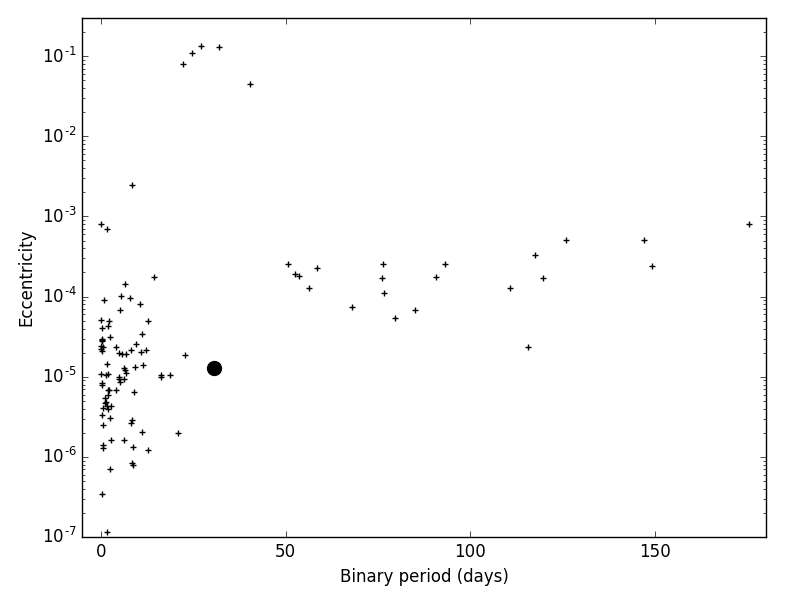
Figure 16: Eccentricity and binary period for every binary MSP that is not in a double neutron star system, globular cluster and does not have a main sequence companion. PSR J1421$-$4409 is identified with a large black circle. It can be seen that its eccentricity is anomalously low for systems in this period range, the so-called “Camilo gap”.

As shown in Figure 16, J1421 falls in the previous identified gap in eccentricity-binary period space, and is indeed more similar to the ordinary PSR-HeWD binaries. For orbital periods larger than 2 days, their evolution is usually well understood, allowing one to derive an orbital period–companion mass relationship (Tauris & Savonije, 1999), which appears to describe the known systems well. Assuming its validity also for J1421, the companion mass should be $\sim 0.28M_{\odot}$. This relatively large value would imply a relatively low orbital inclination angle given the value of the mass function. Assuming a range of pulsar masses between $1.2\leavevmode\nobreak\ \mathrm{M}_{\odot}$ and $1.7\leavevmode\nobreak\ \mathrm{M}_{\odot}$, the implied inclination angle ranges between $38\degree$ and $48\degree$, respectively. One can try to constrain the orbital inclination angle also from the polarisation properties of the pulse profile. If the pulsar’s position angle (PA) swing can be described by a rotating vector model (RVM, Radakrishnan & Cooke 1969), the viewing angle between the spin axis and the line-of-sight to the observer at the closest approach to the magnetic axis, $\zeta$, should be similar to the orbital inclination angle $\zeta\sim i$, if the recycling process spinning up J1421 to its current period led to the expected alignment of orbital angular momentum and spin axis. However, fitting RVMs to recycled pulsars is often difficult, although recent results (e.g. Freire et al., submitted; Berezina et al. submitted) suggest that it is possible in an increasing number of cases. We fitted the RVM to the PA data of J1421 (see Figure 14). We use the PSR/IEEE convention as explained in detail in van Straten et al. (2010), minimizing $\chi^{2}$ for a combination of $\zeta$ and the magnetic inclination angle $\alpha$. The resulting 1-$\sigma$ contours are shown in Figure 14. The best solution implies small $\alpha$ and $\zeta$ values. This is consistent with a wide pulse profile, as observed. However, the data are consistent also with values as large as $\sim 45\degree$. One solution is shown as a solid line in the PA-pulse phase plot below the pulse profile shown in the inset, representing a so-called “inner line of sight” (e.g. Lorimer & Kramer 2005). The data points in light grey have been ignored during the fit and are shown here shifted by $90\degree$ (an “orthogonal jump”) from their original value. Non-orthogonal jumps are not uncommon, but given the low level of the associated linear polarisation they were excluded. Including these data points in the fit, does not change the best fit solution but increases the size of the contours.

The RVM solution corresponds to a combination of angles indicated by the arrow ($\alpha\sim 44\degree$, $\zeta\sim 40\degree$). The solution was chosen as an example for the following reasons. Assuming that the open field-line region of the pulsar is filled with emission, the observed pulse width can be related to $\alpha$ and $\zeta$ and the angular radius of the open field line region, $\rho$. There are indications that this assumption is often not fulfilled for recycled pulsars (Kramer et al., 1998), but it can serve as a useful guide (e.g. Freire et al. submitted). Assuming a period-$\rho$ scaling as found for normal pulsars (e.g. Kramer et al. 1994), we performed Monte-Carlo simulations that result in a distribution of $\alpha$ values consistent with the observed pulse width (see Berezina et al., submitted, for details). Under these assumptions, two ranges of $\alpha$ values are consistent with the data, centred on $50\degree$ and $130\degree$, respectively, as shown in the distribution below the $\alpha$-$\zeta$ plane. Moreover, we can also indicate the range of inclination angles as derived from the Tauris-Savonije relationship, assuming that $\zeta\sim i$. The corresponding range is indicated by the horizontal hashed region. As shown by the arrow, we can find a solution that is consistent with the data and the described constraints. While this is not a unique solution, it does provide a consistent picture of the evolution of the system, the pulse profile and the polarisation information.

5.4 Radio Frequency Interference

The survey has been subject to a large amount of RFI. This comes in many forms — external sources (e.g. satellites, air traffic control radar, malfunctioning observatory equipment), internal sources (e.g. self-induced RFI in individual beams, due to maintenance issues with the multi-beam receiver). RFI is time variable on a number of scales and can be both narrow and broad band. Generally speaking at Parkes, as with most observatories worldwide, the RFI environment is getting worse over time; even the Murchison Radio Observatory site, perhaps the best radio astronomy site on the planet is subject to these effects (Sokolowski et al., 2015). These effects have a strong deleterious effect on our ability to detect astrophysical signals. We are attempting to perform a census of the RFI environment at Parkes using the SUPERB dataset. By characterising the RFI as fully as possible we can improve the quality of our data and thus identify otherwise obscured astrophysical signals (we have had success with this already — see above); this information should be useful to all other users of the observatory also. Here, as an initial illustration of this work, we present several metrics to quantify the effects of RFI in our data. We examine: (i) the number of time-samples removed by our RFI cleaning algorithms after an eigen-value decomposition of the input from all 13 beams — this effects both periodicity and single-pulse searches; (ii) the number of ‘birdies’, i.e. frequencies in the fluctuation spectra that were removed by our algorithms — this effects the periodicity searches; (iii) the number of single-pulse candidates generated — this clearly is only a metric relevant to single-pulse searches. The criteria used for identifying these signals are threshold searches by comparison with the expectation of white noise — in the case of the birdie search an initially ‘de-reddening’ of the fluctuation is performed. These metrics are illustrated in Figures 17 and 18 where we examine altitude and azimuth dependence of these quantities, and their time variability on hourly and monthly timescales. Several patterns are evident in the data, e.g. that RFI is more prevalent during local working hours and contamination is worst for Westerly pointings. A thorough examination of the wide range of RFI signals in the data will be presented in a later paper.

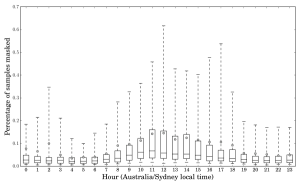
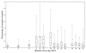
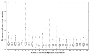
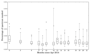
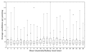
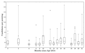
Figure 17: Illustrations of three assessments of the RFI environment at Parkes, as a function of time, during the survey observations reported here. The metrics are shown on hourly (left) and monthly (right) time scales. Top row: The percentage of time samples masked in the eigenvector decomposition based assessment. Middle row: The percentage of spectral bins masked in the ‘birdie’ search. Bottom row: The number of detected single pulse events above a threshold (more than six times the standard deviation in excess of the mean) in each pointing. These metrics are derived from a representative sample of 10000 random survey pointings.

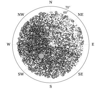
Figure 18: Illustrations of three assessments of the RFI environment at Parkes, as a function of azimuth and zenith for the survey observations reported here. The quantities plotted are the same as in Figure 17: percentage masked samples in the top 2 panels (time samples on the left, frequencies on the right), and number of excess single pulse candidates in the bottom panel. In each panel the centre of each circle is at the position of the single pointing in question and the area of the circle denotes the magnitude of the quantity. Again, these metrics are derived from a random representative sample of 10000 survey pointings.

6 Summary

We have presented the features of SUPERB, an experiment designed for searching for pulsars and fast transients using the multi-beam receiver of the Parkes radio telescope in the 1400-MHz band. The survey exploits a usable bandwidth of $\sim 340$ MHz, split into $390$ kHz wide channels; the integration time is 9-min and the voltages are sampled at $2$ bits every 64 $\upmu$s. In the observations reported here covering the time up to and including January 2016, have accumulated an observing time-field of view product of $\sim 1350$ deg hr (to the half-power sensitivity level), and have tessellated most of the sky visible from Parkes, with particular focus on the intermediate and high Galactic latitudes.

SUPERB has introduced a few significant improvements with respect to the past large scale surveys for pulsar and/or transients carried on at Parkes or elsewhere: (i) the implementation of a real-time search for both periodic (both isolated and binary systems) and transient signals, followed by an offline deeper analysis of all the collected data; (ii) the capability of quickly distributing alerts for the occurrence of transient signals and the associated triggering of a multi-messenger campaign for follow-ups of the transient signals; (iii) the setup of a program of observations shadowing the survey pointings; (iv) the availability of full-Stokes data for transients. Observations are in agreement with the expected limiting sensitivity of the surveys.

Here we have reported on the first 10 pulsar discoveries. One of the two new millisecond pulsars, PSR J1421$-$4407 (6.4 ms spin period) is in a 30.7-d orbit, showing a remarkably small eccentricity in comparison with the other already known systems with a similar orbital period. PSR J1306$-$40 is a 2.2-ms pulsar in an orbit that is as yet unsolved. Indications are that it may be eclipsed by its companion (or associated winds) for a significant fraction of its orbit, and may be similar to the red back binary systems. Further pulsar discoveries, with a particular focus on new ultra-long period pulsars, will be reported in subsequent papers in this series. The next four FRB discoveries (joining the already reported FRB 150418) will be reported in Paper 2. The number of discoveries are roughly in agreement with the expectations based on simple pulsar population models. This will be examined in detail in the future using the SUPERB dataset to include intermittency, scintillation etc. into pulsar population modelling for the first time. SUPERB looks set to continue working successfully and will continue to adapt and improve over time. For example, as new computing capabilities become available and new telescope equipment, such as cooled phased array feeds, come into use, the parameter space searched opens up and the survey gets ever better.

Data Access

Data obtained in this project are archived for long-term storage on the CASS/ANDS data server. These data are publicly available 18 months from the day they are recorded. The data are recorded in sigproc filterbank format, a de facto standard for pulsar search data, and are converted to psrfits format for upload to the data server. From here they can be accessed by anybody. The full resolution data products are produced at a rate of $\sim 46$ MiB/s when observing. For typical observing efficiencies (considering telescope stowing due to wind, RFI or maintenance issues that occur during routine observing) this amounts to $\sim 4$ TB per day of observation.

References

- Ageron et al. (2011) Ageron, M. et al., 2003, Nuclear Instruments and Methods in Physics Research A, 656, 11
- Antoniadis (2014) Antoniadis, J., 2014, ApJ, 797, L24
- Bailes et al. (2011) Bailes M. et al., 2011, Science, 333, 1717
- Bannister et al. (2016) Bannister K. W., Stevens J., Tuntsov A. V., Walker M. A., Johnston S., Reynolds C., Bignall H., 2016, Science, 351, 354
- Barr et al. (2017) Barr E. D. et al., 2017, MNRAS, 465, 1711
- Barsdell et al. (2010) Barsdell B. R., Barnes D. G., Fluke C. J., 2010, MNRAS, 408, 1936
- Bates et al. (2013) Bates S. D., Lorimer D. R., Verbiest J. P. W., 2013, MNRAS, 431, 1352
- Bassa et al. (2016) Bassa C. G. et al., 2016, MNRAS, 463, L36
- Bernlöhr et al. (2003) Bernlöhr K. et al., 2003, Astroparticle Physics, 20, 111
- Braun et al. (2015) Braun R., Bourke T., Green J. A., Keane E., Wagg J., 2015, Advancing Astrophysics with the Square Kilometre Array (AASKA14), 174
- Burke-Spolaor et al. (2011) Burke-Spolaor S., Bailes M., Ekers R., Macquart J.-P., Crawford F., III, 2011, ApJ, 727, 18
- Burke-Spolaor et al. (2011) Burke-Spolaor S. et al., 2011, MNRAS, 416, 2465
- Burrows et al. (2005) Burrows, D. N. et al., 2005, Space Science Reviews, 120, 165
- Caleb et al. (2017) Caleb M. et al., 2017, MNRAS, 468, 3746
- Cameron et al. (2017) Cameron A. D. et al., 2017, MNRAS, 468, 1994
- Camilo (1995) Camilo F., in “The Lives of the Neutron Stars” (NATO ASI Series) Kluwer, Dordrecht, eds. Alpar A., Kiziloglu U., van Paradis J., p. 243.
- Deng et al. (2017) Deng, X. et al., 2017, PASA, 34, 26
- Cordes & Lazio (2002) Cordes & Lazio, 2002, astro-ph/0207156
- Giroletti et al. (2016) Giroletti M. et al., 2016, A&A, 593, L16
- Hallinan et al. (2007) Hallinan G. et al., 2007, ApJ, 663, L25
- Horesh et al. (2015) Horesh A., Cenko S. B., Perley D. A., Kulkarni S. R., Hallinan G., Bellm E., 2015, ApJ, 812, 86
- Hotan et al. (2004) Hotan, A. W., van Straten, W., Manchester, R. N., 2004, PASA, 21, 302
- Hyman et al. (2005) Hyman S. D., Lazio T. J. W., Kassim N. E., Ray P. S., Markwardt C. B., Yusef-Zadeh F., 2005, Nature, 434, 50
- Jankowski et al. (2017) Jankowski F. et al., 2017, MNRAS, in press.
- Johnston et al. (2017) Johnston S. et al., 2017, MNRAS, 465, 2143
- Keane & McLaughlin (2011) Keane E. F., McLaughlin, M. A., 2011, BASI, 39, 333
- Keane et al. (2016) Keane E. F. et al., 2016, Nature, 530, 453
- Keane (2016) Keane E. F., 2016, MNRAS, 459, 1360
- Keith et al. (2010) Keith M. J. et al., 2010, MNRAS, 409, 619
- Keith et al. (2011) Keith M. J. et al., 2011, MNRAS, 419, 1752
- Kocz et al. (2010) Kocz J., Briggs F. H., Reynolds J., 2010, AJ, 140, 2086
- Kondratiev et al. (2009) Kondratiev V. I., McLaughlin M. A., Lorimer D. R., Burgay M., Possenti A., Turolla R., Popov S. B., Zane S., 2009, ApJ, 702, 692
- Kramer et al. (1994) Kramer M., Wielebinski R., Jessner A., Gil J. A., Seiradakis J. H., 1994, A&AS, 107, 515
- Kramer et al. (1998) Kramer M. et al., 1998, ApJ, 501, 270
- Kramer et al. (2006) Kramer M. et al., 2006, Science, 312, 549
- Kramer & Stappers (2015) Kramer M., Stappers B. W., 2015, Advancing Astrophysics with the Square Kilometre Array (AASKA14), 36
- Leshem & van der Veen (2000) Leshem A., van der Veen, A.-J., 2000, Proceedings of “Perspectives on Radio Astronomy: Technologies for Large Antenna Arrays”, ISBN: 90-805434-2-X
- Levin et al. (2013) Levin L. et al., 2013, MNRAS, 434, 1387
- Levin et al. (2010) Levin L. et al., 2010, ApJ, 721, L33
- Linares (2017) Linares, M., 2017, MNRAS submitted, astro-ph/1707.00698
- Lorimer & Kramer (2005) Lorimer D. R., Kramer M., 2005, Handbook of Pulsar Astronomy, CUP
- Lorimer et al. (2007) Lorimer D. R., Bailes M., McLaughlin M. A., Narkevic D. J., Crawford F., 2007, Science, 318, 777
- Lyne et al. (1990) Lyne A. G. et al., 1990, Nature, 347, 650
- Manchester et al. (1990) Manchester, R. N., Hobbs, G. B., Teoh, A., Hobbs, M., 2005, AJ, 129, 1993
- McLaughlin et al. (2006) McLaughlin M. A. et al., 2006, Nature, 439, 817
- Morello et al. (2014) Morello, V., Barr, E. D., Bailes, M., Flynn, C. M., Keane, E. F., van Straten, W., 2014, MNRAS, 443, 1651
- Morello (2016) Morello V., 2016, MSc Thesis, Swinburne University of Technology, “Discovering Pulsars with Machine Learning”
- Osten & Bastian (2008) Osten R. A., Bastian T. S., 2008, ApJ, 674, 1078
- Petroff et al. (2014) Petroff E. et al., 2014, ApJ, 789, L26
- Petroff et al. (2015) Petroff E. et al., 2015, MNRAS, 447, 246
- Petroff et al. (2015) Petroff E. et al., 2015, MNRAS, 451, 3933
- Petroff et al. (2016) Petroff E. et al., 2016, PASA, 33, 45
- Price et al. (2017) Price D. C. et al., 2016, J. Astron. Instrum., 05, 1641007
- Radakrishnan & Cooke (1969) Radakrishnan V., Cooke D. J., 1969, Astrophys. Lett., 3 225
- Ransom et al. (2002) Ransom S. M. et al., 2002, AJ, 124, 1788
- Ransom (2005) Ransom S. M., 2005, Science, 307, 892
- Raza & van der Veen (2002) Raza J. & van der Veen A. J., 2002, IEEE Signal Processing Letters, 9, 64
- Rickett (1970) Rickett B. J., 1970, MNRAS, 150, 67
- Robinson et al. (1995) Robinson C., Lyne A. G., Manchester R. N., Bailes M., D'Amico N., Johnston S., 1995, MNRAS, 274, 547
- Roy et al. (2010) Roy J., Gupta Y., Pen Ue-Li., Peterson J. B., Kudale S., Kodilkar J., 2010, ExA, 28, 25
- Sokolowski et al. (2015) Sokolowski M., Wayth R. B., Morgan, L., 2015, proceedings of GEMCCON, 2015 IEEE Global; doi:/10.1109/GEMCCON.2015.7386856
- Spitler et al. (2016) Spitler L. G. et al., 2016, Nature, 531, 202
- van Straten et al. (2010) van Straten W., Manchester R. N. Johnston S., Reynolds J. E., 2010, PASA, 27, 104
- van Straten (2013) van Straten W., 2013, ApJS, 204, 13
- Staelin (1969) Staelin D. H., 1969, IEEE Proceedings, 57, 724
- Tauris & Savonije (1999) Tauris T. M., Savonije G. J., 1999, A&A, 350, 928
- Thornton et al. (2013) Thornton D. et al., 2013, Science, 341, 53
- Tiburzi et al. (2013) Tiburzi C. et al., 2013, MNRAS, 436, 3557
- Tingay et al. (2013) Tingay, S. J. et al., 2013, PASA, 30, 7
- Williams & Berger (2016) Williams P. K. G., Berger E., 2016, ApJ, 821, L22
- Yao et al. (2017) Yao, M. J., Manchester, R. N., Wang, N., 2017, ApJ, 835, 29