Revisiting ignited-quenched transition and the non-Newtonian rheology of a sheared dilute gas-solid suspension

Abstract

The hydrodynamics and rheology of a sheared dilute gas-solid suspension, consisting of inelastic hard-spheres suspended in a gas, are analysed using anisotropic Maxwellian as the single particle distribution function. The closed-form solutions for granular temperature ($T$) and three invariants of the second-moment tensor are obtained as functions of the Stokes number ($St$), the mean density ($\nu$) and the restitution coefficient ($e$). Multiple states of high and low temperatures are found when the Stokes number is small, thus recovering the “ignited” and “quenched” states, respectively, of Tsao & Koch (J. Fluid Mech.,1995, vol. 296, pp. 211-246). The phase diagram is constructed in the three-dimensional ($\nu,St,e$)-space that delineates the regions of ignited and quenched states and their coexistence. Analytical expressions for the particle-phase shear viscosity and the normal stress differences are obtained, along with related scaling relations on the quenched and ignited states. At any $e$, the shear-viscosity undergoes a discontinuous jump with increasing shear rate (i.e.  discontinuous shear-thickening) at the “quenched-ignited” transition. The first (${\mathcal{N}}_{1}$) and second (${\mathcal{N}}_{2}$) normal-stress differences also undergo similar first-order transitions: (i) ${\mathcal{N}}_{1}$ jumps from large to small positive values and (ii) ${\mathcal{N}}_{2}$ from positive to negative values with increasing $St$, with the sign-change of ${\mathcal{N}}_{2}$ identified with the system making a transition from the quenched to ignited states. The superior prediction of the present theory over the standard Grad’s method and the Chapman-Enskog solution is demonstrated via comparisons of transport coefficients with simulation data for a range of Stokes number and restitution coefficient.

1 Introduction

During the last few decades, a lot of research has been done to understand the behaviours of rapid granular flows (Savage & Jeffrey, 1981; Lun et al., 1984; Jenkins & Richman, 1985; Campbell, 1990; Sela & Goldhirsch, 1998; Brey et al., 1998; Goldhirsch, 2003; Rao & Nott, 2008; Forterre & Pouliquen, 2008), a collection macroscopic inelastic (the restitution coefficient $e<1$) hard-particles for which the effect of the interstitial fluid is neglected, and the tools from dense-gas kinetic theory have been successfully employed to understand its hydrodynamics and rheology. The closely related research-area of gas-solid suspensions (Davidson & Harrison, 1963; Anderson & Jackson, 1968; Buyevich, 1971; Gidaspow, 1994; Jackson, 2000; Guazzelli & Morris, 2011), in which the viscous drag due to interstitial fluid and other related hydrodynamic effects must be incorporated, has also been extensively studied over the last century due to its importance in fluidized-bed and FCC reactors  (Davidson & Harrison, 1963; Gidaspow, 1994) encountered in chemical and process industries. For continuum models of gas-solid suspensions, the kinetic-theory-based rheological models have been suggested by considering elastically colliding particles (Koch, 1990; Tsao & Koch, 1995) as well as for inelastic particles (Louge, Mastorakos & Jenkins, 1991; Sangani et al., 1996; Lun & Savage, 2003) interacting in a bath of a Newtonian gas.

For the present problem of a sheared gas-solid suspension of inelastic particles, the energy input due to shear is compensated by two mechanisms, (i) inelastic inter-particle collisions, characterized by a coefficient of normal restitution ($e$) and (ii) the drag force which the surrounding fluid exerts on the particles. The volume fraction of the suspended particles (of diameter $\sigma$ and mass $m$) is assumed to be small, i.e.  $\nu=\pi\sigma^{3}n/6\ll 1$, representing a ‘dilute’ suspension, along with the conditions of (ii) small Reynolds number $\Rey=\rho_{g}{\dot{\gamma}}\sigma^{2}/\mu_{g}\ll 1$ (where $\rho_{g}$ and $\mu_{g}$ are the gas density and its viscosity, respectively, and ${\dot{\gamma}}$ is the imposed shear rate on the suspension) and (iii) finite Stokes number

$$St={\dot{\gamma}}\tau_{v},\quad\mbox{with}\quad\tau_{v}=m/(3\pi\mu_{g}\sigma)$$ (1)

being the viscous relaxation time which is a measure of the time a typical particle takes to relax back to the local fluid velocity. The limit of $St\to\infty$ represents the ‘dry’ granular gas (Campbell, 1990; Goldhirsch, 2003). Under the above assumptions, Tsao & Koch (1995) analysed the hydrodynamics and the non-Newtonian rheology of a dilute suspension of elastic ($e=1$) hard-particles employing the Grad’s moment-expansion method (i.e. an expansion in terms of Hermite polynomials around a Maxwellian,  Grad (1949)). They discovered two qualitatively different states, dubbed (i) “quenched” (low temperature) and (ii) “ignited” (high temperature) states, corresponding to the time intervals (i) $\tau_{c}\gg\tau_{v}\gg{\dot{\gamma}}^{-1}$ and (ii) $\tau_{c}\ll{\dot{\gamma}}^{-1}\ll\tau_{v}$, respectively, where $\tau_{c}$ is the collision time (i.e, the average time between two successive collisions). They analytically determined two critical Stokes numbers $St_{c_{1}}$ and $St_{c_{2}}$ (with $St_{c_{2}}>St_{c_{1}}$), below and above which the flow remains in the quenched and ignited states, respectively. They also determined the shear viscosity and the first and second normal-stress differences, and compared their theory with DSMC (direct simulation Monte Carlo) data.

Sangani et al. (1996) extended the work of Tsao & Koch (1995) to (i) a ‘dense’ gas-solid suspension of elastic ($e=1$) particles as well as to (ii) a ‘dilute’ suspension of inelastic ($e<1$) particles. The same Grad moment-expansion was used to derive constitutive relations from the underlying Enskog-Boltzmann equation; but their analysis is deficient in the sense that they found zero value for the second normal stress difference as they did not incorporate certain non-linear terms (see §5 in this work). They briefly discussed about the lower limit of Stokes number $St_{c_{1}}$, but a thorough analysis of the “ignited-quenched” transitions, identifying the regions for the existence of different states, in terms of Stokes number ($St$), particle volume fraction ($\nu$) and the coefficient of restitution ($e$) has not been worked out till date. The latter effect of the restitution coefficient is important for dissipative particles which forms one motivation of the present work.

In the current decade, Parmentier, J-F. & Simonin (2012) analysed a sheared gas-solid suspension by considering a distribution function that sandwiches both the ignited and quenched states – the resulting rheological fields are reasonably well-predicted over a range of density and Stokes number, although quantitative mis-match with simulation data exists that increase with increasing dissipation (i.e. at smaller $e$). A Navier-Stokes-order continuum model has been developed by  Garzo et al. (2012) for a moderately-dense gas-solid suspension following dense-gas kinetic theory. They solved the underlying Enskog-Boltzmann equation using a Chapman-Enskog-like expansion around a time-dependent homogeneous cooling state for a gas-solid suspension, and the particle motion has been modelled via a Langevin-type stochastic model with Stokesian drag. The resulting transport coefficients for the particle-phase are found to have explicit dependence on the gas-phase parameters. However, the prediction of the latter model for the shear viscosity of a suspension indicates large discrepancies with simulation data in the dilute limit of low-$St$ suspension, presumably due to the presence of order-one values of normal stress differences and other non-Newtonian effects. A related work to uncover the non-Newtonian rheology of a ‘dilute’ gas-solid suspension has been done recently by  Chamorro, Reyes & Garzo (2015). They followed the standard Grad’s method to analyse the ignited state of a gas-solid suspension, and the related predictions on the granular temperature and the non-Newtonian stress tensor are found to be quantitatively similar to the earlier work of Tsao & Koch (1995); for example, the suspension viscosity is over-predicted by the Grad’s moment-theory at smaller values of $e$, although the discrepancy decreases with increasing Stokes number. Collectively, the above literature review points toward the need to go beyond the well-studied Newtonian rheology (of Navier-Stokes-order) for both dry granular and gas-solid suspensions.

In this paper, we revisit and extend the work of Tsao & Koch (1995) by considering a dilute system of inelastic ($e\leq 1$) particles suspended in a bath of a Newtonian gas, and interacting via (i) a Stokeian drag force and (ii) hard-core inelastic collisions. Our work differs from all previous works on gas-solid suspensions as we adopt the anisotropic Maxwellian distribution function (Goldreich & Tremaine, 1978; Jenkins & Richman, 1988; Richman, 1989) to analyse the underlying Boltzmann equation under homogeneous shearing conditions. The latter assumption is motivated from our recent work (Saha & Alam, 2014, 2016; Alam & Saha, 2017) on ‘dry’ ($St\to\infty$) sheared granular fluid which established that the transport coefficients for highly inelastic system ($e\ll 1$) of a sheared granular fluid (both dilute and dense) can be accurately predicted by the anisotropic Maxwellian [in comparison to (i) the standard Grad’s moment expansion (in terms of a truncated Hermite series around a Maxwellian) as well as (ii) the Burnett-order solutions obtained from Chapman-Enskog expansion]. Here we demonstrate the superiority of the former for the case of a sheared gas-solid suspension via a one-to-one comparison of two theories with simulation data. Another focus of the present work is to analyse and quantify the anisotropy of the second-moment, ${\mathsfb M}=\langle{\boldsymbol{C}}{\boldsymbol{C}}\rangle$, of fluctuation/peculiar velocity, and subsequently tie and explain the rheological/transport coefficients of a sheared gas-solid suspension in terms of the anisotropies of ${\mathsfb M}$. The underlying analysis utilizes the geometric structure of the eigen-basis of both the shear tensor and the second-moment tensor; this provides geometric insight into the origin of normal stress differences as found for the case of a sheared granular fluid (Saha & Alam, 2016). It must be noted that the analysis of stress anisotropy in this form was initiated in a seminal work by Goldreich & Tremaine (1978) and subsequently by others (Araki & Tremaine, 1986; Araki, 1988; Shukhman, 1984; Jenkins & Richman, 1988; Richman, 1989) and the present effort is a continuation of the same legacy to the case of a sheared gas-solid suspension.

This paper is organized as follows. A brief account of the problem and the governing equations for the gas and particle phases are given in §2. The anisotropic-Maxwellian distribution function is introduced in §2.1 which is employed to analyse the “ignited” state of sheared gas-solid suspension; the second moment tensor for the uniform shear flow is constructed in §2.1.1 in terms of its eigen-basis. The source term of the second moment balance equation is calculated in §2.1.2 and §2.2 for the ignited and quenched states, respectively. The second-moment balance combining both ignited ($I$) and quenched ($Q$) states is analysed in §2.3. The multi-stability and hysteresis transitions in granular temperature are analysed in detail in §3, along with (i) the validation and superiority of the present analysis in §3.1, (ii) analytical solutions for temperatures in three states in §3.2 and (iii) the critical Stokes numbers for “$I\leftrightarrow Q$” transitions in §3.3. The non-Newtonian rheology (shear-thickening, normal stress differences) is analysed in §4.2 and §4.3, in terms of the anisotropies of the second-moment tensor (§4.1). The relative merits of the present theory over the standard Grad’s moment-expansion and Chapman-Enskog expansion are analysed in §5 via comparisons with available simulation data. The conclusions are given in §6. The mathematical details of various analyses are relegated to Appendices A to F.

2 Problem description and the kinetic-theory analysis

We examine the uniform shear flow of a dilute gas-solid suspension in the absence of gravity, with a collection of smooth inelastic spheres of mass $m$ and diameter $\sigma$ being suspended in a gas; with $x$, $y$ and $z$ pointing the velocity, gradient and vorticity directions (see figure 1), respectively, the velocity field for the suspension is given by

$${\boldsymbol{u}}\equiv(u_{x},u_{y},u_{z})=(\dot{\gamma}y,0,0),$$ (2)

where $\dot{\gamma}$ is the overall shear rate. We are interested in a steady state suspension where the fluid inertia is very small but the particle inertia remains finite. Under the assumptions of the smallness of particle Reynolds number, the gas-phase obeys the Stokes equations of motion

$$\mu_{g}\nabla^{2}v_{i}=\nabla_{i}p_{g},\qquad\nabla_{i}v_{i}=0,$$ (3)

where $\mu_{g}$ is the shear viscosity of the gas. The velocity profile (2) satisfies (3).

For the particle-phase, we adopt the kinetic theory of granular gases (Chapman & Cowling, 1970; Jenkins & Richman, 1985; Sela & Goldhirsch, 1998; Brey et al., 1998; Brilliantov & Pöschel, 2004). Any physical quantity at the macroscopic level is defined as the ensemble averaged value of the same at the particle level, using the single particle distribution $f({\boldsymbol{c}},{\boldsymbol{x}},t)$ function

$$\langle\psi({\boldsymbol{c}})\rangle\equiv\frac{1}{n}\int\psi{\boldsymbol{c}}f({\boldsymbol{c}},{\boldsymbol{x}},t)d{\boldsymbol{c}},$$ (4)

with $\psi({\boldsymbol{c}})$ being any particle-level quantity. Here $n\equiv n({\boldsymbol{x}},t)$ denotes the number density and $\rho({\boldsymbol{x}},t)=mn\equiv\rho_{p}\nu$ is the mass-density of the particle-phase, with $\nu$ being the volume fraction of particles and $\rho_{p}=m/(\pi\sigma^{3}/6)$ is its intrinsic/material density. The macroscopic/hydrodynamic velocity ${\boldsymbol{u}}=\langle{{\boldsymbol{c}}}\rangle$, the granular temperature $T=\langle{{\boldsymbol{C}}^{2}/3}\rangle$ and the particle-phase stress tensor ${\boldsymbol{P}}=\langle{m{\boldsymbol{C}\boldsymbol{C}}}\rangle$ are obtained by substituting $\psi={\boldsymbol{c}},\;\frac{1}{3}{\boldsymbol{C}}^{2}\;{\rm and}\;m{\boldsymbol{C}C}$, respectively, in (4), where ${\boldsymbol{C}}={\boldsymbol{c}}-{\boldsymbol{u}}$, is the peculiar velocity.

For a dilute suspension ($\nu\ll 1$), the evolution of the single particle distribution function $(f({\boldsymbol{c}},{\boldsymbol{x}},t))$ follows the celebrated Boltzmann equation (Chapman & Cowling, 1970)

$$\left(\frac{\partial}{\partial t}+{\boldsymbol{c}}\cdot\nabla\right)f+\nabla_{\boldsymbol{c}}\cdot\left(f\frac{{\rm d}{\boldsymbol{c}}}{{\rm d}t}\right)=\Big{(}\frac{\partial f}{\partial t}\Big{)}_{coll},$$ (5)

where $\nabla_{\boldsymbol{c}}$ is divergence operator in the velocity space; the acceleration of the particles is assumed to follow the Stokes’s linear drag law:

$$\frac{{\rm d}{\boldsymbol{c}}}{{\rm d}t}=-\frac{{\boldsymbol{c}}-{\boldsymbol{v}}}{\tau_{v}},$$ (6)

with $\tau_{v}=m/(3\pi\mu_{g}\sigma)$ being the viscous relaxation time of the particles. Equation (6) holds if the particle Reynolds number and the density-ratio ($\rho_{f}/\rho_{p}$) are very small; for large Reynolds numbers, a nonlinear form of the drag-law would be necessary. The hydrodynamic interactions have been neglected throughout the present analysis – the particles are assumed to follow the fluid velocity, i.e., there is no slip (${\boldsymbol{v}}={\boldsymbol{u}}$). These additional effects and a complete analysis of the particle-phase rheology in the dense limit (based on Enskog equation) will be considered in a future work.

For the present problem of the steady homogeneous shear flow, the mass-density $\rho$, the velocity gradient ${\boldsymbol{\nabla}u}\propto{\dot{\gamma}}$ and the stress tensor ${\mathsfb P}$ are constants and the heat flux vanishes. In this case the balance equations for mass and linear momentum are identically satisfied and the balance of the second moment of fluctuation velocity, ${\mathsfb M}=\langle{{\boldsymbol{C}\boldsymbol{C}}}\rangle$, reduces to

$${\mathsfb P}\cdot\nabla{\boldsymbol{u}}+\left({\mathsfb P}\cdot\nabla{\boldsymbol{u}}\right)^{T}+\frac{2{\dot{\gamma}}}{St}{\mathsfb P}={\boldsymbol{\aleph}},$$ (7)

where $St=\dot{\gamma}\tau_{v}$ is the Stokes number and ${\boldsymbol{\aleph}}$ is the source (collisional production) of second moment, given by (Jenkins & Richman, 1985; Saha & Alam, 2014)

$${\boldsymbol{\aleph}} = \int m{\boldsymbol{C}}{\boldsymbol{C}}\Big{(}\frac{\partial f}{\partial t}\Big{)}_{coll}d{\boldsymbol{C}}=\frac{\sigma^{2}}{2}\int\Delta\Big{(}m{\boldsymbol{C}}{\boldsymbol{C}}\Big{)}f({\boldsymbol{C}}_{1})f({\boldsymbol{C}}_{2})d{\boldsymbol{C}}_{1}d{\boldsymbol{C}}_{2},$$ (8)

with

$$\Delta\Big{(}m{\boldsymbol{C}}{\boldsymbol{C}}\Big{)}=-\frac{m}{2}(1+e)({\boldsymbol{g}}\cdot{\boldsymbol{k}})\left[(1-e)({\boldsymbol{g}}\cdot{\boldsymbol{k}}){\boldsymbol{k}}{\boldsymbol{k}}+({\boldsymbol{j}}{\boldsymbol{k}}+{\boldsymbol{k}}{\boldsymbol{j}}){\boldsymbol{g}}{\boldsymbol{j}}\right],$$ (9)

where ${\boldsymbol{g}}={\boldsymbol{c}}_{1}-{\boldsymbol{c}}_{2}$ is the relative velocity between two colliding particles $1$ and $2$; ${\boldsymbol{k}}\equiv{\boldsymbol{k}}_{12}=({\boldsymbol{x}}_{1}-{\boldsymbol{x}}_{2})/|{\boldsymbol{x}}_{1}-{\boldsymbol{x}}_{2}|$ is the unit contact vector joining the center of particle-$1$ to that particle-$2$, and ${\boldsymbol{j}}$ is its normal.

With an appropriate choice of the distribution function $f({\boldsymbol{c}},{\boldsymbol{x}},t)$, the collision integral (8) can be evaluated, which will be plugged into (7) to carry out the analysis for the particle-phase rheology and hydrodynamics of a sheared gas-solid suspension.

2.1 Analysis in the ignited sate

The “ignited” state (Tsao & Koch, 1995) represents the hydrodynamic state of fluidized-particles in rapid granular flow (Goldhirsch, 2003), where the particles fly around randomly in between two collisions without getting much affected by the viscous drag of the interstitial fluid. A typical particle encounters successive collisions with other particles again and again before it can relax back to the local fluid velocity and hence the collision time is much smaller than the viscous relaxation time ($\tau_{c}\ll\tau_{v}$). In this state, the particles have strong velocity fluctuations, resulting in $T/\dot{\gamma}\sigma\gg 1$.

As in our recent work (Saha & Alam, 2014, 2016), the distribution function in the ignited state of a sheared suspension is assumed to be an anisotropic Maxwellian,

$$f({\boldsymbol{c}},{\boldsymbol{x}},t)=\frac{n}{(8\pi^{3}|{\mathsfb M}|)^{1/2}}{\rm exp}\Big{(}-\frac{1}{2}{\boldsymbol{C}}\cdot{\mathsfb M}\cdot{\boldsymbol{C}}\Big{)},$$ (10)

where $|{\mathsfb M}|=det({\mathsfb M})$. This form of the distribution function has been used previously in studying the velocity dispersions in Saturn’s rings (Goldreich & Tremaine, 1978; Shukhman, 1984; Araki & Tremaine, 1986; Araki, 1988) as well as to analyse the shear flow of dry rapid granular flows (Jenkins & Richman, 1988; Richman, 1989; Lutsko, 2004).

In the isotropic limit, (10) reduces to the Maxwellian distribution function, and an Hermite expansion of the form

$$f({\boldsymbol{c}},{\boldsymbol{x}},t) = \frac{n}{(2\pi T)^{3/2}}{\rm exp}\Big{(}-C^{2}/2T\Big{)}\sum_{i}a^{(i)}{\mathcal{H}}^{(i)}$$ (11)

$$= \frac{n}{(2\pi T)^{3/2}}{\rm exp}\Big{(}-C^{2}/2T\Big{)}\Big{\{}1+\frac{1}{2\rho T^{2}}P_{\langle\alpha\beta\rangle}C_{\alpha}C_{\beta}\Big{\}}+HOT,$$

represents the well-known Grad’s moment expansion (GME) (Grad, 1949) – such moment expansion has subsequently been employed to solve the Boltzmann equation for molecular gases (Herdegen & Hess, 1982; Kremer, 2010), granular gases (Jenkins & Richman, 1985; Kremer & Marques, 2011) and gas-solid suspensions (Tsao & Koch, 1995; Sangani et al., 1996; Chamorro, Reyes & Garzo, 2015). Equation (11) with leading-order term ($P_{\langle\alpha\beta\rangle}=\rho M_{\alpha\beta}-T\delta_{\alpha\beta}$ is the stress deviator) yields the 10-moment system of Grad (1949), with density, velocity, temperature and stress-deviator constituting the extended set of ten hydrodynamic fields (Saha & Alam, 2016).

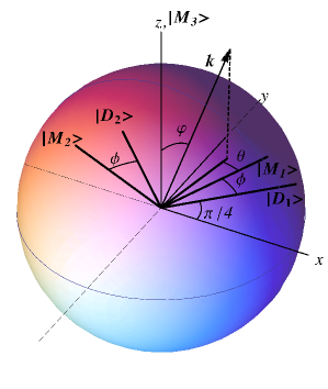
Figure 1: Schematic of the co-ordinate system and the eigen-basis for analysis; the eigen-directions of the shear tensor ${\mathsfb D}$ and the second moment tensor ${\mathsfb M}$ are decpicted. The uniform shear flow, ${\boldsymbol{u}}=({\dot{\gamma}}y,0,0)$, is directed along the $x$-direction, with the velocity gradient along the $y$-direction and the mean-vorticity along the $z$-direction.

2.1.1 Uniform shear flow (USF) and the second moment tensor

The analysis in this section closely follows the theoretical framework introduced by (Goldreich & Tremaine, 1978; Shukhman, 1984; Araki & Tremaine, 1986; Jenkins & Richman, 1988; Richman, 1989). For the uniform shear flow, the velocity gradient tensor can be decomposed as

$$\bnabla{{\boldsymbol{u}}}={\mathsfb D}+{\mathsfb W}\equiv\left[\begin{array}[]{ccc}0&\dot{\gamma}/2&0\\ \dot{\gamma}/2&0&0\\ 0&0&0\end{array}\right]\quad+\quad\left[\begin{array}[]{ccc}0&\dot{\gamma}/2&0\\ -\dot{\gamma}/2&0&0\\ 0&0&0\end{array}\right],$$ (12)

where $\mathsfb D$ and $\mathsfb W$ are the shear and spin tensors, respectively. Referring to figure 1, the ($x,y$)-plane is dubbed the shear plane and the $z$-direction is the vorticity direction. The eigenvalues of ${\mathsfb{D}}$ are $\dot{\gamma}/2$, $-\dot{\gamma}/2$ and $0$, with the corresponding orthonormal eigenvectors, respectively,

$$|D_{1}\rangle=\left[\begin{array}[]{ccc}\cos\frac{\pi}{4}\\ \sin\frac{\pi}{4}\\ 0\end{array}\right],\quad|D_{2}\rangle=\left[\begin{array}[]{ccc}-\sin\frac{\pi}{4}\\ \>\>\>\cos\frac{\pi}{4}\\ 0\end{array}\right]\quad\mbox{and}\quad|D_{3}\rangle=\left[\begin{array}[]{ccc}0\\ 0\\ 1\end{array}\right],$$ (13)

that are sketched in figure 1. While $|D_{3}\rangle$ is directed along the $z$-axis, the shear-plane eigenvectors $|D_{1}\rangle$ and $|D_{2}\rangle$ are rotated by $45\,^{\circ}$ anticlockwise from the $xy$-axes.

Since the granular temperature $T=M_{\alpha\alpha}/3$ is the isotropic measure of the second moment tensor $\mathsfb{M}=\langle{\boldsymbol{C}}{\boldsymbol{C}}\rangle$, we can decompose it as ${\mathsfb{M}}/{T}={\mathsfb I}+{\widehat{\mathsfb{M}}}/{T}$, where $\widehat{\mathsfb{M}}/T$ is the dimensionless counterpart of its deviatoric/traceless tensor. The eigenvalues of ${\mathsfb{M}}$ are denoted by $T(1+\xi)$, $T(1+\varsigma)$ and $T(1+\zeta)$, with $\xi$, $\varsigma$ and $\zeta$ being the eigenvalues of $\widehat{\mathsfb{M}}/T$ such that

$$\xi+\varsigma+\zeta=0.$$ (14)

The corresponding orthonormal set of eigen-directions are assumed to be $|M_{1}\rangle$, $|M_{2}\rangle$ and $|M_{3}\rangle$, respectively, as depicted in figure 1. Therefore, the second-moment tensor ${\mathsfb{M}}$ can be written in terms of its eigen-basis:

$$\mathsfb{M}=T(1+\xi)|M_{1}\rangle\langle M_{1}|+T(1+\varsigma)|M_{2}\rangle\langle M_{2}|+T(1+\zeta)|M_{3}\rangle\langle M_{3}|.$$ (15)

Referring to figure 1, we assume that the shear-plane eigenvectors $|M_{1}\rangle$ and $|M_{2}\rangle$ can be obtained by rotating the system of axes at an angle $(\pi/4+\phi)$, with $\phi$ being unknown, in the anti-clockwise sense about the $z$-axis which coincides with $|M_{3}\rangle$:

$$|M_{1}\rangle=\left[\begin{array}[]{ccc}\cos\left(\phi+\frac{\pi}{4}\right)\\ \sin\left(\phi+\frac{\pi}{4}\right)\\ 0\end{array}\right],\quad|M_{2}\rangle=\left[\begin{array}[]{ccc}-\sin\left(\phi+\frac{\pi}{4}\right)\\ \>\>\>\cos\left(\phi+\frac{\pi}{4}\right)\\ 0\end{array}\right]\quad\mbox{and}\quad|M_{3}\rangle=\left[\begin{array}[]{ccc}0\\ 0\\ 1\end{array}\right].$$ (16)

We further assume that the contact vector ${{\boldsymbol{k}}}$ makes an angle $\varphi$ with $|M_{3}\rangle$, and $\theta$ is the angle between $|M_{1}\rangle$ and ${\boldsymbol{k}}-({\boldsymbol{k}}\bcdot{\boldsymbol{z}}){\boldsymbol{z}}$, the projection of ${\boldsymbol{k}}$ on the shear plane, as shown in figure 1. Inserting (16) into (15), we obtain the following expression for the second moment tensor

$$\mathsfb{M}=T[\delta_{\alpha\beta}]+\widehat{\mathsfb M},$$ (17)

with its deviatoric part being given by

$$\widehat{\mathsfb M}=T\left[\begin{array}[]{ccc}\lambda^{2}+\eta\sin 2\phi&-\eta\cos 2\phi&0\\ -\eta\cos 2\phi&\lambda^{2}-\eta\sin 2\phi&0\\ 0&0&-2\lambda^{2}\end{array}\right].$$ (18)

Here we have introduced the following notations

$$\eta\equiv\frac{1}{2}(\varsigma-\xi)\geq 0\quad\mbox{and}\quad\lambda^{2}\equiv\frac{1}{2}(\varsigma+\xi)=-\frac{\zeta}{2}\geq 0,$$ (19)

such that the eigenvalues in the shear-plane can be expressed in terms of $\eta$ and $\lambda$ via

$$\xi=\lambda^{2}-\eta\quad\mbox{and}\quad\varsigma=\lambda^{2}+\eta>\xi,$$ (20)

with the eigenvalue, $\zeta$, along the vorticity direction ($z$), being given by (19).

Since $\phi=0$ implies that the shear tensor (${\mathsfb D}$) and the second-moment tensor (${\mathsfb M}$) have same principal directions, a non-zero value of $\phi$ is a measure of the non-coaxiality angle between the principal directions of ${\mathsfb D}$ and ${\mathsfb M}$. It is straightforward to show that $\eta\sim(T_{x}-T_{y})$ is proportional to the difference between two temperatures $T_{x}$ and $T_{y}$ on the shear-plane ($x,y$), and hence $\eta\neq 0$ is indicative of the degree of temperature-anisotropy on the shear plane. On the other hand, a non-zero value of $\lambda^{2}$ is a measure of the excess temperature (Saha & Alam, 2016),

$$T^{ex}_{z}=(T-T_{z})=2\lambda^{2}T\quad\Rightarrow\;\;\lambda^{2}=\frac{T^{ex}_{z}}{2T},$$ (21)

along the mean vorticity direction. In summary, the anisotropy of ${\mathsfb M}$ is quantified in terms of three dimensionless quantities: (i) $\eta\propto(T_{x}-T_{y})\neq 0$, or, $\phi\neq 0$ and (ii) $\lambda^{2}\propto T_{z}^{ex}\neq 0$.

The second-moment tensor (17-18) in the USF of suspension, constructed from its eigen-basis, is therefore completely determined when $T$, $\eta$, $\phi$ and $\lambda^{2}$ are specified; the dependence on the Stokes number $St$ and the particle volume fraction ($\nu$) is implicit as will be made clear below.

2.1.2 Source term in the ignited state

Employing (10), the collisional production term (8) for the ignited state has been evaluated

$$\aleph_{\alpha\beta}^{is}=-\frac{6(1+e)\rho_{p}\nu^{2}}{\upi^{\frac{3}{2}}\sigma}\Big{\{}(1-e)\int k_{\alpha}k_{\beta}(\boldsymbol{k}\cdot{\mathsfb M}\cdot\boldsymbol{k})^{\frac{3}{2}}d\boldsymbol{k}$$

$$\hskip 113.81102pt+2\int(k_{\alpha}j_{\beta}+j_{\alpha}k_{\beta})(\boldsymbol{k}\cdot{\mathsfb M}\cdot\boldsymbol{k})^{\frac{1}{2}}(\boldsymbol{k}\cdot{\mathsfb M}\cdot\boldsymbol{j})d\boldsymbol{k}\Big{\}}.$$ (22)

$$\qquad=-\frac{4(1+e)\rho_{p}\nu^{2}T^{3/2}}{35\sigma\sqrt{\pi}}\Big{\{}(1-e)\times$$

$$\left[\begin{array}[]{ccc}70+9\eta^{2}+42\lambda^{2}+42\eta\sin 2\phi&-42\eta\cos 2\phi&0\\ -42\eta\cos 2\phi&70+9\eta^{2}+42\lambda^{2}-42\eta\sin 2\phi&0\\ 0&0&70+3\eta^{2}-84\lambda^{2}\end{array}\right]$$ (26)

$$\quad+\;4\left[\begin{array}[]{ccc}\eta^{2}+21\lambda^{2}+21\eta\sin 2\phi&-21\eta\cos 2\phi&0\\ -21\eta\cos 2\phi&\eta^{2}+21\lambda^{2}-21\eta\sin 2\phi&0\\ 0&0&-2(\eta^{2}+21\lambda^{2})\end{array}\right]\Big{\}},$$ (30)

which is a function of $\nu$, $e$, $T$, $\eta$, $\phi$ and $\lambda^{2}$. In the final expression (30), we have retained terms that are up-to second-order in $\eta$, $\sin\phi$ and $\lambda$ – we shall show in the end that this is sufficient to yield accurate predictions of transport coefficients of a sheared dilute suspension.for a wide range of (i) restitution coefficient $e$ and (ii) Stokes number $St$.

2.2 Analysis in the quenched sate

Tsao & Koch (1995) envisaged a scenario of a dilute gas-solid suspension in which the particle inertia is very low such that the particles tend to align with fluid streamlines after a collision. Most of the particles will be having their individual velocity equal to the fluid velocity $({\boldsymbol{c}}\approx{\boldsymbol{u}})$ which implies that the peculiar velocity ${\boldsymbol{C}}\approx 0$ and therefore the particle agitation is very small ($T/\dot{\gamma}\sigma\ll 1$) – this is dubbed the quenched state. The collisions in this state are mainly shear-induced with some occasional variance-driven collisions and the particles relax back to the local fluid velocity after such a collision before they encounter a second collision and therefore the viscous relaxation time is much smaller than the collision time $\tau_{v}\ll\tau_{c}$. The velocity distribution function of the quenched state is taken to be a delta function

$$f=n\delta({\boldsymbol{C}}),$$ (31)

which is a solution of the Boltzmann equation. Using (31), the collisional production term at second-order can be evaluated as

$$\aleph_{\alpha\beta}^{qs} = -\rho{\dot{\gamma}}^{3}\sigma^{2}\frac{3(1+e)^{2}\nu}{2\upi}\int_{k_{x},k_{y}>0}(k_{x}k_{y})^{3}k_{\alpha}k_{\beta}d\boldsymbol{k},$$ (35)

$$= \rho_{p}{\dot{\gamma}}^{3}\sigma^{2}\frac{(1+e)^{2}\nu^{2}}{16}\left[\begin{array}[]{ccc}\frac{512}{315\upi}&-\frac{16}{35}&0\\ -\frac{16}{35}&\frac{512}{315\upi}&0\\ 0&0&\frac{128}{315\upi}\end{array}\right].$$

Note that this expression differs from that of Tsao & Koch (1995) by a numerical-factor $2$ which was also noted previously (Parmentier, J-F. & Simonin, 2012).

2.3 Second moment balance combining quenched and ignited states

Combining the ignited and quenched states, the second-order moment balance equation (7) for a ‘dilute’ gas-solid suspension undergoing uniform shear flow is

$$P_{\delta\beta}u_{\alpha,\delta}+P_{\delta\alpha}u_{\beta,\delta}+\frac{2\dot{\gamma}}{St}P_{\alpha\beta}=\aleph_{\alpha\beta}\equiv\aleph_{\alpha\beta}^{qs}+\aleph_{\alpha\beta}^{is},$$ (36)

where the superscripts $qs$ and $is$ stand for the source of second moment in quenched and ignited states, respectively. Following (17-18), the expression for the stress tensor can be written as

$${\mathsfb P}=\rho{\mathsfb M}=\rho_{p}\nu T\left[\begin{array}[]{ccc}1+\lambda^{2}+\eta\sin 2\phi&-\eta\cos 2\phi&0\\ -\eta\cos 2\phi&1+\lambda^{2}-\eta\sin 2\phi&0\\ 0&0&1-2\lambda^{2}\end{array}\right].$$ (37)

Substituting (22), (35) and (37) into (36), we obtain the following four independent equations:

$$\left.\begin{array}[]{rcl}-2T\eta\cos 2\phi+\frac{2}{St}T(1+\lambda^{2}+\eta\sin 2\phi)&=&\Big{[}-\frac{2(1-e^{2})\nu T^{\frac{3}{2}}}{35\sqrt{\upi}}(70+9\eta^{2}+42\lambda^{2}+42\eta\sin 2\phi)\\ &&-\frac{8(1+e)\nu T^{\frac{3}{2}}}{35\sqrt{\upi}}(\eta^{2}+21\lambda^{2}+21\eta\sin 2\phi)\Big{]}\\ &&+\Big{[}\frac{128(1+e)^{2}\nu}{315\pi}\Big{]},\\ \frac{2}{St}T(1+\lambda^{2}-\eta\sin 2\phi)&=&\Big{[}-\frac{2(1-e^{2})\nu T^{\frac{3}{2}}}{35\sqrt{\upi}}(70+9\eta^{2}+42\lambda^{2}-42\eta\sin 2\phi)\\ &&-\frac{8(1+e)\nu T^{\frac{3}{2}}}{35\sqrt{\upi}}(\eta^{2}+21\lambda^{2}-21\eta\sin 2\phi)\Big{]}\\ &&+\Big{[}\frac{128(1+e)^{2}\nu}{315\pi}\Big{]},\\ \frac{2}{St}T(1-2\lambda^{2})&=&\Big{[}-\frac{2(1-e^{2})\nu T^{\frac{3}{2}}}{35\sqrt{\upi}}(70+3\eta^{2}-84\lambda^{2})\\ &&+\frac{16(1+e)\nu T^{\frac{3}{2}}}{35\sqrt{\upi}}(\eta^{2}+21\lambda^{2})\Big{]}+\Big{[}\frac{32(1+e)^{2}\nu}{315\pi}\Big{]},\\ T(1+\lambda^{2}-\eta\sin 2\phi)-\frac{2}{St}T\eta\cos 2\phi&=&\Big{[}\frac{12(1-e)(3-e)\nu T^{\frac{3}{2}}}{5\sqrt{\upi}}\eta\cos 2\phi-\frac{4(1+e)^{2}\nu}{35\pi}\Big{]}.\end{array}\right\},$$ (38)

Note that the terms involving the Stokes number ($St$) on the left-hand sides of (38) vanish in the limit of $St\to\infty$, thereby recovering the second-moment balance for the shear flow of a ‘dry’ granular gas (Saha & Alam, 2016).

In (38), we have made temperature dimensionless via $T=T/(\dot{\gamma}\sigma/2)^{2}$. The coupled system of equations (38) must be solved to determine $\eta$, $\lambda$, $\phi$ and $T$ for specified values of (i) particle volume fraction ($\nu$), (ii) Stokes number ($St$) and (iii) restitution coefficient ($e$). Analytical progress can be made to solve (38) as discussed in §3 and §4.

Before proceeding further, it may be noted that the analysis of the second moment balance (36) or (38) in the ignited state (i.e. with $\aleph_{\alpha\beta}^{qs}=0$) is considerably simplified for elastically-colliding ($e=1$) particles, see Appendix A. The related analytical results on the temperature field provide a lower-bound on the Stokes number for the existence of the ignited state (and consequently on the multiple states and hysteresis, §3.2) in a dilute gas-solid suspension.

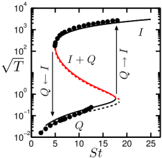
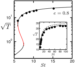
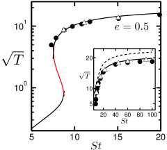
(a) (b) (c) (d)

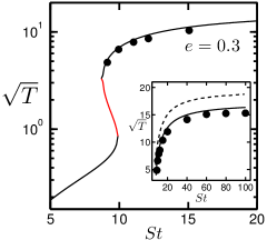
Figure 2: Hysteretic/first-order transitions of granular temperature for (a) $e=1$ and $\nu=5\times 10^{-4}$; (b) $e=0.8$, (c) $e=0.5$ and (d) $e=0.3$ with $\nu=0.01$. The solid and dashed (inset) lines denote the present anisotropic-Maxwellian theory and the Maxwellian theory (Tsao & Koch, 1995; Sangani et al., 1996), respectively. The filled-circles represent the DSMC data of Sangani et al. (1996); the open-triangles in panel $c$ denote the DSMC data of Chamorro, Reyes & Garzo (2015). In each panel, the black and red lines represent stable and unstable solutions, respectively, of Eq. (3.1).

3 Granular temperature: Multi-stability and ignited-to-quenched state transitions

After some tedious algebra, we found that (38) can be decoupled to yield a $10$-th degree polynomial for granular temperature $\xi=\sqrt{T}$:

$$\mathcal{G}(\xi)\equiv a_{10}\xi^{10}+a_{9}\xi^{9}+a_{8}\xi^{8}+a_{7}\xi^{7}+a_{6}\xi^{6}+a_{5}\xi^{5}+a_{4}\xi^{4}+a_{3}\xi^{3}+a_{2}\xi^{2}+a_{1}\xi+a_{0}=0,$$ (39)

the explicit expressions of the coefficients $a_{i}$ are given in Appendix B. It is straightforward to verify that for the case of elastically colliding particles ($e=1$), $a_{10}=0=a_{9}=a_{8}$ and hence (39) reduces to a polynomial of 7th-degree; in fact these three roots vapourize to $-\infty$ at $e=1$ and remain negative for $e<1$ and hence unphysical. It has been verified numerically (as well as via an ordering analysis, see Appendix B) that at most three roots of (39) are real positive, depending on the values of $\nu$, $St$ and $e$, and the remaining roots are negative and/or complex.

3.1 Validation of present anisotropic-Maxwellian theory

First, we solve the temperature equation (39) numerically and compare it with simulation data in order to validate the present theory.

Figure 2(a,b,c,d) shows the variations of the granular temperature with Stokes number $(St)$ at particle volume fractions of $(a)$ $\nu=5\times 10^{-4}$ and $(b,c,d)$ $\nu=0.01$, with different values of the restitution coefficient (a) $e=1$, (b) $e=0.8$, (c) $e=0.5$ and $e=0.3$. In each panel and inset, the symbols represent the DSMC (direct simulation Monte Carlo) data of Sangani et al. (1996) which are compared with the (i) present anisotrpic-Maxwellian theory (solid line) and (ii) the standard moment expansion (dashed line) of Tsao & Koch (1995, for $e=1$) and Sangani et al. (1996, for $e\neq 1$), Figure 2($a$) indicates that for the case of elastically colliding particles, the present theory is on par with Tsao-Koch theory. On the other hand, for inelastic particles ($e<1$), the insets of figure 2(b,c,d) confirm that the present theory is able to better predict the temperature-variation with $St$; however, the agreement with Tsao-Koch theory worsens with increasing dissipation. In panel $c$, the recent DSMC data (open triangles) of Chamorro, Reyes & Garzo (2015) for $e=0.5$ also agree quantitatively with the present theory.

Overall, the moment theory with anisotropic-Maxwellian as the leading term seems better suited for a dilute gas-solid suspension of inelastic particles undergoing shear flow for a large range of $e<1$ at small and moderate values of Stokes number. It may be noted that a similar analysis (Saha & Alam, 2014, 2016) for a sheared granular gas ($St=\infty$) provides excellent predictions for temperature and rheological quantities for highly dissipative particles. The same conclusions seem to carry over to the limit of small Stokes numbers of a sheared gas-solid suspension too – this issue is further discussed in §5 (with respect to predictions for viscosity and normal stress differences).

3.2 Analytical solution for three temperatures: hysteresis and multi-stability

Returning to figure 2, we note that the temperature is a multi-valued function of Stokes number for a range of $St$ over which there are three possible solutions; there are hysteretic/discontinuous jumps in temperature from the low/high temperature branches with increasing/decreasing $St$. For a better understanding of this hysteresis phenomenon, equation (39) has been solved in the asymptotic limit $\nu\ll 1$, $St\gg 1$, and $St^{3}\nu\ll 1$ via an ordering analysis, the details of which are given in Appendix C. Three real solutions have been found,

$$\sqrt{T_{is}} = \frac{5(1+e)^{-1}(1691+539e-1223e^{2}+337e^{3})\sqrt{\upi}}{48(3-e)(12607-19952e+10099e^{2}-1746e^{3})}\left(\frac{St}{\nu}\right)\;\stackrel{{\scriptstyle e=1}}{{\equiv}}\;\frac{5\sqrt{\pi}}{144}\frac{St}{\nu},$$ (40)

$$\sqrt{T_{qs}} = \sqrt{\frac{32(1+e)^{2}}{945\upi}}St^{3/2}\nu^{1/2}\;\stackrel{{\scriptstyle e=1}}{{\equiv}}\;\frac{8\sqrt{2}}{3\sqrt{105\pi}}St^{3/2}\nu^{1/2},$$ (41)

$$\sqrt{T_{us}} = \frac{840\sqrt{\upi}}{(1+e)(107+193e)}\left(\frac{1}{St^{3}\nu}\right)\;\stackrel{{\scriptstyle e=1}}{{\equiv}}\;\frac{7\sqrt{\pi}}{5}\left(\frac{1}{St^{3}\nu}\right),$$ (42)

which correspond to the temperatures in the ignited ($T_{is}$), quenched ($T_{qs}$) and unstable ($T_{us}$) states, respectively. These three solutions (40-42) can be identified in figure 2 as the high-, low-, and intermediate-temperature branches, respectively; the red-colored solution branch in each panel of figure 2 represent $T_{us}$ which is of course unstable from stability viewpoint (see §4.2 for related discussions).

It is clear from (40) that $T_{is}$ increases with increasing Stokes number $St$, but decreases with increasing particle volume fraction $\nu$. On the other hand, the quenched-state temperature (41) increases with increasing $St$ and $\nu$, whereas the unstable temperature (42) decreases with increasing $St$ and $\nu$. These overall predictions are verified in figure 3 which display the variations of granular temperature as functions of ($\nu,e$) for two values of Stokes number (a) $St=10$ and (b) $St=20$. In each panel, the upper-most branch corresponds to the ignited-state of high temperature $T_{is}$; the middle and the lower-most planes represent the unstable and quenched states, respectively. The latter two states are connected via a line of turning-points, resulting in saddle-node bifurcations (jump-transitions) from “$Q\to I$” with increasing $\nu$, above which the ignited state is the only solution. The critical density $\nu=\nu_{c}(St,e)$ for this transition increases with increasing inelasticity but decreases with increasing $St$ (see panel $b$). The corresponding Stokes number for “$Q\to I$”-transition is denoted by $St_{c_{2}}(\nu,e)$ which can also be identified with the right limit-point in figure 2.

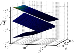
(a) (b)

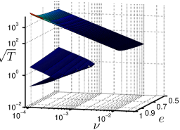
Figure 3: Multiple states of granular temperature as functions of the mean volume fraction $\nu$ and restitution coefficient $e$ for (a) $St=10$ and (b) $St=20$.

A noteworthy feature of figure 3 is that the ignited branch [$T\propto\nu^{-2}$, see (40)] is disconnected from the quenched and unstable branches, and therefore there is no jump-transitions (on decreasing $\nu$) from $I\to Q$ at $St=10$ (panel $a$) and $20$ (panel $b$). However, on further decreasing the Stokes number (below $St=10$), the ignited state solution disappears below a minimum $St$ – how this process occurs is explained in figures 4(a,b,c) for $e=1$, $0.8$ and $0.5$, respectively. In particular, at any $e$, the unstable branch (red line) and the ignited-branch come closer with decreasing $St$ and merge with each other at some minimum $St$ below which only the quenched-state solution [$T\propto\nu$, see (41)] survives. Similarly, by fixing the Stokes number at $St=6$ but increasing the inelasticity (decreasing $e$) also results in the disappearance of the ignited state solution, see figure 4(d). Therefore, the quenched state is the only possible solution below a minimum Stokes number $St=St_{c_{1}}(e,\nu)$ – this can be identified with the left limit-point in figure 2 for “$I\to Q$” transition.

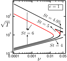
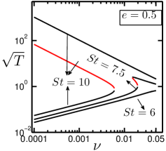
(a) (b)
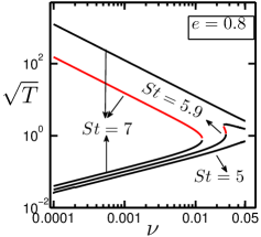
(c) (d)

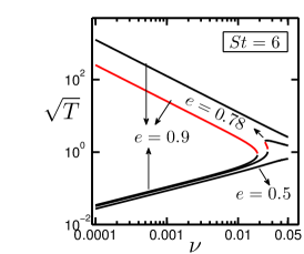
Figure 4: Disappearance of the ignited-state branch with (a,b,c) decreasing Stokes number at (a) $e=1$, (b) $e=0.8$ and (c) $e=0.5$, and (d) the same with decreasing restitution coefficient at $St=6$.

3.3 Critical Stokes numbers ($St_{c_{1}},St_{c_{2}}$) and the master phase-diagram

Referring to figure 2, two critical/limit points (at $St=St_{c_{1}}$ and $St_{c_{2}}$, with $St_{c_{2}}>St_{c_{1}}$) correspond to the double roots of (39) at which the following conditions must be satisfied:

$$\mathcal{G}(\xi_{c})=0\quad\mbox{and}\quad\mathcal{G}^{\prime}(\xi_{c})=0.$$ (43)

This implies that two solution branches, corresponding to two different states [(i) ignited $(T_{is})$, (ii) quenched $(T_{qs})$ and (iii) unstable $(T_{us})$] meet at $\xi=\xi_{c}$, leading to saddle-node bifurcations from one stable state to another stable state.

The discontinuous “$Q\to I$” transition corresponds to a limit point ($St=St_{c_{2}}$, viz. figure 2$a$) at which the quenched and unstable solution branches meet. Carrying out the asymptotic analysis of (39) with $T_{qs}=T_{us}$ and satisfying (43) (see Appendix D for details), we obtain the following relation

$$St_{c_{2}}^{3}\nu_{c}=\Bigg{(}\frac{3087000\pi^{2}}{(1+e)^{4}(107+193e)^{2}}\Bigg{)}^{\frac{1}{3}},$$ (44)

that represents a critical-surface in the ($\nu,St,e$)-plane, above which only the ignited state exists. Equation (44) is depicted in figure 5 as a blue-surface. In the elastic limit of $e=1$, (44) reduces to $St_{c_{2}}^{3}\nu_{c}=2.7685$ which differs from the prediction $(\approx 3.23)$ of Tsao & Koch (1995).

The critical Stokes number, $St_{c_{1}}$, for the “$I\to Q$” transition (on decreasing $St$) corresponds to the limit point at which $T_{is}=T_{us}$. The asymptotic analysis of (39) yields the following expression for $St_{c_{1}}$ (see Appendix D for details):

$$St_{c_{1}}\approx 9.9-4.91e,$$ (45)

which is marked as a brown-shaded plane in figure 5, to the left of which only the quenched state exists. For elastically colliding particles ($e=1$), we have $St_{c_{1}}\approx 4.99$ which is close to our numerical solution of $4.94...$; both are close to the result of $\sqrt{169.5/7}\approx 4.92$ obtained by Tsao & Koch (1995). Note that (45) depends only on the restitution coefficient, and therefore the minimum value of Stokes number $(St_{c_{1}})$, below which only the quenched-state exists, is independent of the volume fraction for a dilute gas-solid suspension.

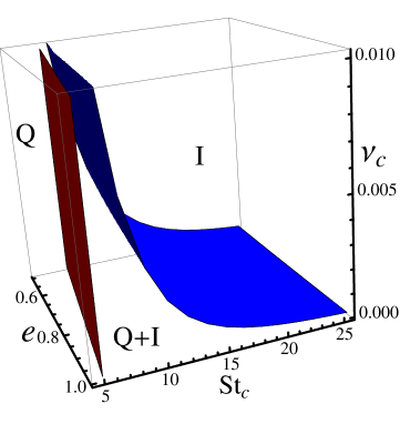
Figure 5: Complete phase diagram of different states [“ignited” (I), “quenched” (Q) and their coexistence (Q+I)] in the ($\nu,St,e$)-plane. The blue- and brown-colored planes, above and below which, respectively, the ignited and quenched states exist, have been determined analytically from an ordering analysis of (3.1) in the dilute limit; for details, see the text in §3.3 and Appendix D.

The master phase-diagram in figure 5 summarizes all possible states in the ($\nu,St,e$)-plane: (i) the ignited state ($I$) exists above the blue-surface, (ii) the quenched state ($Q$) is the only solution to the left of the brown surface and (iii) the coexistence of ignited and quenched ($I+Q$) states occurs for parameter values lying between the blue and brown surfaces. Two critical surfaces in figure 5 would meet along a curve, thus acting as an upper bound for the existence of the unstable state ($T_{us}$) solution (and hence the existence of the mixed state $I+Q$). By equating $St_{c_{1}}=St_{c_{2}}$, the equation of this curve is obtained as

$$\nu_{us}^{l}(e)=\Bigg{(}\frac{3087000\pi^{2}}{(1+e)^{4}(107+193e)^{2}}\Bigg{)}^{\frac{1}{3}}/{(9.9-4.91e)^{3}},$$ (46)

which is a decreasing function of the restitution coefficient. Note that (46) is not a critical point, rather it represents an upper-bound on density below which the phase-coexistence [$I+Q$] occurs in the small-$St$ regime of a sheared gas-solid suspension.

It is clear from from (45) and (44) that the critical Stokes numbers $St_{c_{1}}$ and $St_{c_{2}}$ increase with decreasing $e$ (i.e.  increasing inelasticity) at a fixed volume fraction $\nu<\nu_{us}^{l}$, When dissipative particles ($e\ll 1$) collide with each other they loose more energy and hence loose more of their inertia; in that case the recovery time $(\tau_{v})$ reduces and the adjustment with the local fluid velocity becomes faster, leading to the quenched state. On the other hand, for nearly elastic ($e\sim 1$) collisions, the particles lose very little kinetic energy during collisions and take much more time to come back to the bulk flow and hence the recovery process becomes slow. Therefore, at higher values of $e$, both ignited and quenched states exist but only the quenched state is possible if we increase inelasticity of the system, leading to the behaviour of $St_{c_{1}}$ as in (45). Similar argument holds for the variation of $St_{c_{2}}$ with inelasticity as well.

4 Non-Newtonian rheology: second-moment anisotropy, discontinuous shear-thickening and normal stress differences

Once the temperature field is solved from (39) for specified values of $\nu$, $St$ and $e$, the non-coaxiality angle $\phi$, the temperature-anisotropy $\eta$ and the excess temperature $\lambda^{2}$ can be calculated from the remaining equations of (38) – these are amenable to analytical solutions as described in §4.1. The behaviour of shear viscosity and normal stress differences are analysed in §4.2 and §4.3, respectively.

4.1 Anisotropies of second-moment tensor: analytical solution for $\phi$, $\eta$ and $\lambda^{2}$

After some algebra and rearrangement of terms in (38), the closed-form solutions for $\phi$, $\eta^{2}$ and $\lambda^{2}$ have been found:

$$\phi = \frac{1}{2}\tan^{-1}\left(\frac{2}{St}+\frac{12(1+e)(3-e)\nu\sqrt{T}}{5\sqrt{\pi}}\right)^{-1},$$ (47)

$$\eta^{2} = -\frac{\mathfrak{b}}{2\mathfrak{a}}-\frac{1}{2\mathfrak{a}}\sqrt{{\mathfrak{b}}^{2}-4{\mathfrak{a}}{\mathfrak{c}}},$$ (48)

$$\lambda^{2} = \frac{\frac{5\sqrt{\pi}}{2St}T+(1+e)\nu T^{3/2}[5(1-e)-(5+3e)\frac{\eta^{2}}{14}]-\frac{8(1+e)^{2}\nu}{63\sqrt{\pi}}}{\left(\frac{5\sqrt{\pi}}{St}T+{6(1+e)(3-e)\nu T^{3/2}}\right)},$$ (49)

with $T$ being calculated from (39) for specified values of $St$, $\nu$ and $e$. The solution for the temperature-anisotropy $\eta$ follows from the quadratic equation ${\mathfrak{a}}\eta^{4}+{\mathfrak{b}}\eta^{2}+{\mathfrak{c}}=0$, where

$$\left.\begin{array}[]{lcl}{\mathfrak{a}}&=&\frac{9(1-e^{2})^{2}\nu^{2}T^{3}}{25{\pi}}>0\\ {\mathfrak{b}}&=&\frac{6(1-e^{2})\nu T^{3/2}}{5\sqrt{\pi}}\left(\frac{3}{St}T-\frac{16\nu(1+e)^{2}}{35\pi}+\frac{6(1-e^{2})\nu T^{3/2}}{\sqrt{\pi}}\right)-T^{2}\cos^{2}{2\phi}\\ {\mathfrak{c}}&=&\left(\frac{3}{St}T-\frac{16\nu(1+e)^{2}}{35\pi}+\frac{6(1-e^{2})\nu T^{3/2}}{\sqrt{\pi}}\right)^{2}>0\end{array}\right\}.$$ (50)

For a suspension of elastically colliding particles ($e=1$, with finite $St$), we have ${\mathfrak{a}}=0$ and ${\mathfrak{b}}=-T^{2}\cos^{2}{2\phi}$, and hence the above solutions (47-49) simplify to

$$\left.\begin{array}[]{rcl}\phi(e=1)&=&\frac{1}{2}\tan^{-1}\left(\frac{2}{St}+\frac{48\nu\sqrt{T}}{5\sqrt{\pi}}\right)^{-1}>0,\\ \eta^{2}(e=1)&=&-\frac{{\mathfrak{c}}}{\mathfrak{b}}\equiv\left(\frac{3}{St}T-\frac{64\nu}{35\pi}\right)^{2}T^{-2}\sec^{2}{2\phi}>0,\\ \lambda^{2}(e=1)&=&\frac{\frac{5\sqrt{\pi}}{2St}T-\frac{8}{7}\nu T^{3/2}\eta^{2}-\frac{32\nu}{63\sqrt{\pi}}}{\left(\frac{5\sqrt{\pi}}{St}T+{24\nu T^{3/2}}\right)}>0.\end{array}\right\}$$ (51)

Recall from (2.17) that the non-zero values of ($\phi,\eta,\lambda^{2}$) quantify the degree of anisotropy of the second-moment tensor $\mathsfb{M}$ (and hence is a measure of the anisotropy of the kinetic stress tensor, $\mathsfb{P}=\langle\rho{\boldsymbol{C}}{\boldsymbol{C}}\rangle=\rho\mathsfb{M}$, too).

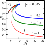
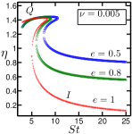
(a) (b) (c)

Figure 6: Variations of (a) the non-coaxiality angle $\phi$, (b) the shear-plane anisotropy $\eta$ and (c) the excess temperature $\lambda^{2}$ with Stokes number for different $e$. The mean volume fraction is set to $\nu=0.005$.

The positivity of (47-49) is verified in figures 6(a), 6(b) and 6(c), respectively, which display the variations of $\phi$, $\eta$ and $\lambda^{2}$ with Stokes number for different values of the restitution coefficient $e\leq 1$, at a mean volume fraction of $\nu=0.005$ – the results look qualitatively similar at other values of $\nu<\nu_{us}^{l}$ (46). It is seen from figure 6 that the increasing inelasticity markedly increases the values of ($\phi,\eta,\lambda^{2}$) on the ignited state, thereby enhancing the anisotropy of the second-moment tensor. In contrast, the inelasticity does not noticeably affect ($\phi,\eta,\lambda^{2}$) on the quenched state in which the particle collisions are rare and the dynamics is primarily dictated by fluid inertia. Interestingly, increasing shear makes the second-moment tensor more anisotropic on the quenched branch – this can be understood by considering the scaling relations of ($\phi,\eta,\lambda^{2}$) at $St\sim 0$ as follows. Using the closed-form solutions for three temperatures (3.2-3.4), the non-coaxiality angle for $e=1$ can be rewritten as

$$\tan{2\phi_{qs}}=\frac{St}{2+\frac{128\sqrt{2}}{5\sqrt{105}\pi}\nu^{3/2}St^{5/2}}\sim St/2\quad\mbox{at}\quad St\sim 0.$$ (52)

Therefore, in the limit of small $St$, the inertia enhances the non-coaxiality angle in the quenched state. On the other hand, increasing $St$ decreases $\phi$ in the ignited state, reaching some asymptotic value (depending on $e$) at large enough $St$ as seen in figure 6(a). This can be explained from an analysis of the ignited branch solution, leading to:

$$\tan{2\phi_{is}}=\frac{3St}{6+St^{2}}\sim\frac{3}{St},\quad\mbox{for}\quad St\gg 1.$$ (53)

Similar scalings (52-53) hold for the temperature anisotropy $\eta$ and the excess temperature $\lambda^{2}$ too, that explain the observed behaviour in figures 6(b) and 6(c), respectively. In summary, the degree of anisotropy of the second-moment tensor in the quenched and ignited states is primarily dictated by the background shear and inelasticity, respectively. The latter effect of inelasticty can be understood from following scaling arguments.

It may be noted that the scaling relation (53) is not strictly valid at $St\to\infty$ since the double-limit of $e\to 1$ and $St\to\infty$ leads to a singular behaviour of temperature $T\to\infty$ (and hence a thermostat is necessary to achieve a steady shearing state of elastically colliding particles in the absence of fluid drag). The case of a sheared granular gas ($St=\infty$ at $e\neq 1$) has been analysed previously (Jenkins & Richman, 1988; Richman, 1989; Saha & Alam, 2014, 2016); it can be verified that the above solutions (47-49) for the ignited-branch reduce to the low-density solution of Saha & Alam (2016):

$$\left.\begin{array}[]{rcl}\lambda^{2}&\approx&\frac{1}{48e}\left(168+53(1-e)\right)\left[\sqrt{1+5760e(1-e)(168+53(1-e))^{-2}}-1\right]\\ &\approx&\frac{5}{14}(1-e)\left(1+\frac{53}{168}(1-e)\right)\left(1-\frac{53}{84}(1-e)\right)\\ \eta^{2}&=&\frac{3\lambda^{2}(7+6\lambda^{2})}{6+\lambda^{2}}\approx\frac{7}{2}\lambda^{2}=\frac{5}{4}(1-e)\left(1+\frac{53}{168}(1-e)\right)\left(1-\frac{53}{84}(1-e)\right)\\ \sin{2\phi}&=&\frac{\eta}{1+\lambda^{2}}\approx\eta\sim\sqrt{1-e}\\ \sqrt{T}&=&\frac{5\sqrt{\pi}\eta\cos{\phi}}{3(1-e^{2})\nu(10+\eta^{2})}\approx\frac{\sqrt{\pi}}{6(1-e^{2})\nu}\eta(1-\eta^{2}/10)(1-\eta^{2}/2)\\ &\approx&\frac{\sqrt{\pi}}{6(1-e^{2})\nu}\eta(1-\frac{3}{5}\eta^{2})\sim(1-e)^{-1/2}\end{array}\right\}$$ (54)

Therefore, in the limit ($St\to\infty$) of a granular gas, $\eta\sim\lambda\sim\sin{2\phi}\sim\sqrt{(}1-e)$, with the granular temperature diverging like $T\sim(1-e)^{-1}$ – the latter finding rules out the possibility of the quenched-state solution in a sheared granular gas. The scaling relations (54) hold at leading-order in $\sqrt{1-e}$ for $St\gg 1$, and therefore we conclude that the inelasticty enhances the degree of anisotropy of ${\mathsfb M}$ on the ignited branch, see figure 6.

(a)

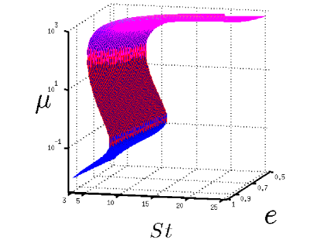
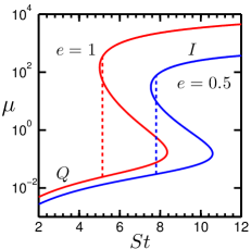
(b) (c)

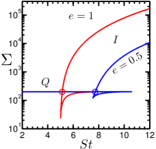
Figure 7: (a) Hysteretic behaviour of particle-phase viscosity ($\mu$) as functions of ($St,e$) for a volume fraction of $\nu=0.005$; this represents DST (discontinuous shear-thickening) behaviour for any $e$ at $\nu<\nu_{us}^{l}$ [(3.8)]. (b) Viscosity versus $St$ for $e=1$ (red line) and $e=0.5$ (blue line); the vertical dotted lines represent the coexistence-point, marked by circles in panel $c$, at which two states $I$ and $Q$ coexists with each other. (c) An effective Massieu function (58), with parameter values as in panel $b$; see the text for details.

4.2 Shear viscosity: continuous and discontinuous shear-thickening (DST)

The dimensionless shear viscosity for the particle phase is given by

$$\mu = -\frac{P_{xy}}{\rho_{p}\nu(\dot{\gamma}\sigma/2)^{2}}=\eta\cos(2\phi)T$$ (55)

$$\equiv \frac{3}{St}T-\frac{16\nu(1+e)^{2}}{35\pi}+\frac{3(1-e^{2})\nu T^{3/2}}{5\sqrt{\pi}}(10+\eta^{2}),$$

$$\stackrel{{\scriptstyle St\to\infty}}{{\equiv}} -\frac{16\nu(1+e)^{2}}{35\pi}+\frac{3(1-e^{2})\nu T^{3/2}}{5\sqrt{\pi}}(10+\eta^{2})>0,\qquad\forall\quad e<1.$$ (56)

For the ignited-state solution only (i.e. $\aleph\equiv\aleph^{is}$), it can be verified that the shear viscosity for elastically colliding particles ($e=1$) is $\mu={3T}/{St}$ which represents the first term in (55).

The variation of (55) as functions of ($St,e$) is depicted in figure 7(a) for particle volume fraction of $\nu=0.005$. Similar to granular temperature, the shear viscosity undergoes hysteretic jumps at $St=St_{c_{2}}$ (“$Q\to I$”) and $St_{c_{1}}$ (“$I\to Q$”) on increasing and decreasing $St$, respectively. The effect of dissipation ($e<1$) is to reduce the viscosity of the particle-phase in each state, see figure 7(b). On the other hand, the effect of Stokes number can be understood by considering the viscosity of elastically colliding ($e=1$) particles as given by

$$\mu_{is} \approx \frac{75\pi}{20736}\frac{St}{\nu^{2}},\quad\mu_{qs}\approx\frac{384}{945\pi}\nu St^{2},\quad\mbox{and}\quad\mu_{us}\approx\frac{147\pi}{25}\nu^{-2}St^{-7},$$ (57)

in the ignited, quenched and unstable states, respectively. Clearly, two shear-thickening branches ($Q$ and $I$) are connected via a shear-thinning branch.

The ‘discontinuous shear thickening’ (DST) behaviour, such as in figure 7(a,b), occurs only in the small Stokes-number limit of a dilute gas-solid suspension at $\nu<\nu_{us}^{l}$, (46), for any restitution coefficient. The middle-branch in figure 7(a,b), over which $\mu$ decreases with increasing $St$ (i.e. the shear-thinning branch), is unstable. This is a thermodynamic/constitutive instability which can be understood from a phenomenological viewpoint. Let us calculate the following quantity,

$$\Sigma(\dot{\gamma})=\int_{\dot{\gamma}_{R}}^{\dot{\gamma}}\mu(\dot{\gamma})\dot{\gamma}{\rm d}\dot{\gamma}+\Sigma_{R},$$ (58)

which is a measure of the stress work and the reference value $\Sigma_{R}$ is added to make $\Sigma(\dot{\gamma})$ positive definite. The variation of (58) is plotted against $St$ in figure 7(c) for $e=1$ (red line) and $0.5$ (blue line). For each case, the upper-most envelope in figure 7(c) represents the stable solution, and the intersection between the ignited and quenched branches represent the coexistence point at which both states coexist with each other. The latter point is marked by vertical dashed lines in figure 7(b) – this also follows from the well-known Maxwell’s equal-area rule. For the present problem, the effective shear work (58) behaves like a Massieu function (Callen, 1985) for the selection of the ‘coexisting’ solution branch, although it must be noted that the choice of (58) is not unique. For example, if we choose to probe the jump in dynamic friction, $\mu/p$, the location of the coexisting branch gets slightly shifted (not shown). A proper identification of a Massieu/entropy function, or, a thermodynamic potential for the present sheared suspension may require a stability analysis of the underlying moment equations subject to uniform shear flow, which is left to a future work.

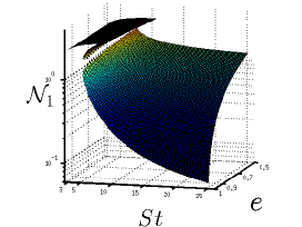
(a) (b)

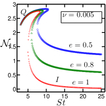
Figure 8: Variations of the first $({\mathcal{N}}_{1})$ normal stress differences against Stokes number ($St$) and restitution coefficient ($e$) at $\nu=0.005$. In panel $b$ the projection of panel $a$ is displayed for different $e$.

In the area of liquid-solid suspensions, the shear-thickening and its discontinuous analog are well-known since the original work of Hoffman (1972). There have been a renewed research activity to understand the origin of DST in the “dense” regime of colloidal and non-colloidal suspensions as well as in dense granular media (Brown & Jaeger, 2014; Denn & Morris, 2014). Extending the present theoretical formalism to the dense regime of suspensions, by incorporating frictional interactions and related physics (Seto et al., 2013; Fernandez et al., 2013; Wyart & Cates, 2014; Clavaud et al., 2017), would be an interesting future work. We became aware of a recent work that uses gas kinetic theory (Hayakawa & Takada, 2016) in the context of a dilute “thermerlized” granular gas, and their finding on DST as a “saddle-node” bifurcation is similar to the present findings (Saha & Alam, 2016a) – however, they did not refer to the work of Tsao & Koch (1995) from which the present work follows. How a thermalized granular gas is related to present system of a gas-solid suspension needs to be investigated.

4.3 First and second normal stress differences

The expression for the first normal stress difference is

$${\mathcal{N}}_{1} = \frac{P_{xx}-P_{yy}}{p}=2\eta\sin{2\phi},$$ (59)

which has been ‘scaled’ by the mean pressure $p=(P_{xx}+P_{yy}+P_{zz})/3$; in (59), $\phi$ and $\eta$ are calculated from (47) and (48), respectively. The variation of (59) as functions of ($St,e$) is displayed in figure 8(a,b). The quenched-branch ${\mathcal{N}}_{1}$ remains unaffected by inelasticity (see panel b), however, on the ignited branch, increasing inelasticity increases ${\mathcal{N}}_{1}$; the effect of the gas-phase (i.e. decreasing $St$) also increases the ignited branch ${\mathcal{N}}_{1}$. On the whole, the dependence of ${\mathcal{N}}_{1}$ on both $St$ and $e$ mirrors that of the non-coaxiality angle ($\phi$) and the shear-plane temperature-anisotropy ($\eta$), compare figure 8(b) with figure 6(a,b). It is clear from (59) that the origin of the first normal stress difference is tied to the shear-plane anisotropies ($\eta$ and $\phi$) of the second-moment tensor as in the case of a sheared granular gas (Jenkins & Richman, 1988; Saha & Alam, 2016) – the dependence of $St$ on its origin remains implicit via two anisotropy parameters ($\phi,\eta$).

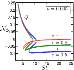
(a) (b)

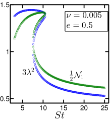
(c)

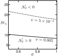
Figure 9: (a) Variation of the second $({\mathcal{N}}_{2})$ normal stress difference against Stokes number $(St)$ for different values of the restitution coefficient; the particle volume fraction is $\nu=0.005$. (b) Variations of $3\lambda^{2}$ (blue circles) and ${\mathcal{N}}_{1}/2$ (green triangles) with $St$ for $e=0.5$, with other parameters as in panel $a$. (c) Variations of the critical Stokes number $St_{\pm}$ (at which ${\mathcal{N}}_{2}=0$) with $e$ for $\nu=0.005$ (solid line) and $\nu=0.0005$ (dashed line).

The scaled second normal stress difference is given by

$${\mathcal{N}}_{2} = \frac{P_{yy}-P_{zz}}{p}=3\lambda^{2}-\eta\sin{2\phi}=3\lambda^{2}-\frac{1}{2}{\mathcal{N}}_{1}.$$ (60)

The variation of (60) with $St$ is shown in figure 9(a) for different values of the restitution coefficient $e$. Similar to ${\mathcal{N}}_{1}$, the effect of inelasticity is to increase the magnitude of the second normal stress difference on the ignited branch, but the quenched-branch ${\mathcal{N}}_{2}$ remains unaffected (expectedly) by changing $e$. It is noteworthy in figure 9(a) that ${\mathcal{N}}_{2}$ is positive and negative in the quenched and ignited states, respectively. This sign-change can be understood from figure 9(b) which display the variations of two terms in (60) with $St$. In the quenched state the excess temperature ($3\lambda^{2}\propto T_{z}^{ex}$) dominates over the shear-plane anisotropies ($\eta\sin{2\phi}\equiv{\mathcal{N}}_{1}/2$), whereas the latter dominates over the former in the ignited state, resulting in the sign-change of ${\mathcal{N}}_{2}$ at some finite value of $St$.

The parameter combinations ($St,e,\nu$) at which ${\mathcal{N}}_{2}$ undergoes sign-reversal can be calculated by solving the following equation

$${\mathcal{N}}_{1}-6\lambda^{2}=0,$$ (61)

along with (59) and (49). Figure 9(c) shows the variation of $St_{\pm}$ with restitution coefficient: ${\mathcal{N}}_{2}$ is positive and negative, respectively, below and above each line for a specified density $\nu$. It is seen that the effect of inelastic dissipation is to increase the critical value of $St_{\pm}$ at which ${\mathcal{N}}_{2}$ changes its sign; reducing the mean-density increases $St_{\pm}$ at any $e$.

It may be noted that for a ‘dense’ sheared granular gas ($St\to\infty$), the second normal-stress difference undergoes sign-change (Alam & Luding, 2005; Saha & Alam, 2016) at some critical density ($\nu_{\pm}\sim 0.2$), with ${\mathcal{N}}_{2}$ being negative and positive in the dilute and dense limit, respectively; the competition between (i) the collisional anisotropies in a dense system (that makes the particle-motion increasingly streamlined (Alam & Luding, 2005) with increasing density) and (ii) the second-moment anisotropies ($\phi,\eta,\lambda^{2}$) is known to be responsible for this sign-change (Saha & Alam, 2016). For the present case of a ‘dilute’ suspension, the behaviour of ${\mathcal{N}}_{2}$ in the quenched state resembles that in a sheared ‘dense’ granular fluid; this could possibly be due to the ‘streamlined’ particle motion in both systems, characterizing the underlying anisotropy.

5 Discussion: Comparison with Grad’s moment-expansion (GME)

Recall that in figure 2, we have made a detailed comparison between the predictions of two moment theories: (i) the standard Grad’s moment-expansion (GME) around a Maxwellian (Grad, 1949; Tsao & Koch, 1995; Sangani et al., 1996; Chamorro, Reyes & Garzo, 2015) using Hermite polynomials and (i) the present anisotropic-Maxwellian moment-expansion (AME). Overall, the AME predictions for granular temperature are found to be more accurate (see insets in figure 2) than that of GME, especially at lower values of restitution coefficient, via a comparison with available simulation data. This conclusion holds for shear viscosity too (not shown) since $\mu\propto\sqrt{T}$ – in the following we focus on the predictive abilities of the present theory (AME) with reference to two normal-stress differences. (The reader is referred to Saha & Alam (2014) for details on AME that has been used to derive a generalized Fourier law for heat-flux vector, along with conductivity tensors; the heat-flux, however, vanishes in uniform shear flow as in the present case.)

5.1 Suspension of elastic and inelastic hard spheres: ${\mathcal{N}}_{1}$ and ${\mathcal{N}}_{2}$

From the present AME theory, the normal stress differences for elastic ($e=1$) hard-sphere suspensions in the “ignited” state are given by (Appendix A)

$$\mathcal{N}_{1}=\frac{18}{6+\Omega St^{2}}\quad\mbox{and}\quad-\mathcal{N}_{2}=\frac{9(9+\Omega St^{2})\Omega St^{2}}{(6+\Omega St^{2})\left[252+{87}\Omega St^{2}+{7}\Omega^{2}St^{4}\right]}>0.$$ (62)

with

$$\Omega=\frac{1}{2St^{2}}\left[\left(St^{2}-\frac{171}{7}\right)+\left(\left(St^{2}-\frac{3}{7}\right)^{2}-(12\sqrt{2})^{2}\right)^{1/2}\right].$$ (63)

The last quantity $\Omega$ is positive for $St>St_{c_{1}}=\sqrt{171/7}$ (the critical Stokes number for “ignited-to-unstable” transition, viz. eqn. (3.7)), and asymptotically approaches unity, $\Omega(St\to\infty)=1$, and hence $\Omega\in(0,1)$ at any $St>St_{c_{1}}$.

The AME-predictions (62) can be compared with the corresponding GME predictions for ${\mathcal{N}}_{1}$ and ${\mathcal{N}}_{2}$:

$${\mathcal{N}}_{1}=\frac{18}{6+\Theta St^{2}}\quad\mbox{and}\quad-{\mathcal{N}}_{2}=\frac{\frac{9}{14}\Theta}{6+\Theta St^{2}}>0,$$ (64)

where

$$\Theta=\frac{1}{2St^{2}}\left[\left(St^{2}-\frac{171}{14}\right)+\left(\left(St^{2}-\frac{171}{14}\right)^{2}-12^{2}\right)^{1/2}\right].$$ (65)

In (64) that there is a minor correction in the expression for ${\mathcal{N}}_{2}$: the numerical factor $9/14$ in the numerator was taken as $9/7$ in Tsao & Koch (1995). The positivity of (65) follows from the positivity of its discriminant, resulting in $St>St_{c_{1}}=\sqrt{169.5/7}$, which is very close to $\sqrt{171/7}$ for the positivity of (63). It is worth pointing out that the functional dependence of both (63) and (65) yields almost identical values for $\Omega$ and $\Theta$ at any $St>St_{c_{1}}$.

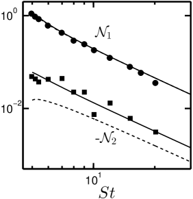
Figure 10: Variations of the first (circles) and second (squares) normal-stress differences with Stokes number for a suspension of elastic ($e=1$) hard-spheres – the particle volume fraction is $\nu=0.01$, representing a ‘dilute’ suspension. The solid lines represent the present theory (62) and the dashed lines represent the standard Grad’s moment theory (64); the DSMC simulation data (Tsao & Koch, 1995) are denoted by symbols.

Figure 10 shows a comparison of (62) (denoted by solid lines) for ${\mathcal{N}}_{1}$ and ${\mathcal{N}}_{2}$ with (i) the DSMC simulation data (symbols) of Tsao & Koch (1995) and (ii) the GME theory (64) (dashed lines) – the particle volume fraction is set to $\nu=0.01$, representing a ‘dilute’ gas-solid suspension. It is seen that both (62) and (64) predict the correct behaviour of ${\mathcal{N}}_{1}$ – two theories are almost indistinguishable from each other, with excellent quantitative agreement with simulation. However, there is a significant disagreement (by a factor of about $2$) between (64) and the DSMC data for the second normal-stress difference ${\mathcal{N}}_{2}$; in contrast, the predictions of AME (62) are uniformly good for both ${\mathcal{N}}_{1}$ and ${\mathcal{N}}_{2}$ over a range of Stokes number.

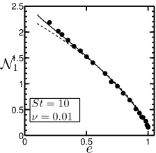
(a) (b)

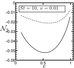
Figure 11: Comparisons of (a) first and (b) second normal-stress differences at $St=10$: (i) DSMC simulation (filled circles, Sangani et al. (1996)), (ii) present theory (solid lines), (iii) the standard Grad’s moment expansion [dashed lines, see Appendix E].

It may be noted that in GME the quadratic nonlinear-terms (proportional to $P_{\alpha\beta}^{2}$) need to be taken into account while evaluating the source term $\aleph_{\alpha\beta}$ (8) in order to obtain ‘non-zero’ second normal-stress difference as suggested by Herdegen & Hess (1982) for a Boltzmann (dilute) gas. A brief account of the related analysis for a gas-solid suspension of inelastic particles is provided in Appendix E – the resulting expressions for ${\mathcal{N}}_{1}$ and ${\mathcal{N}}_{2}$ reduce to (64) for elastically-colliding particles. On the other hand, the analysis of Sangani et al. (1996) did not include such nonlinear Grad-terms, resulting in ${\mathcal{N}}_{2}=0$; the recent work of Chamorro, Reyes & Garzo (2015) also confirmed that the nonlinear Grad-terms are necessary for ${\mathcal{N}}_{2}\neq 0$. It has been verified that the quadratic non-linear terms do not noticeably affect the value of ${\mathcal{N}}_{1}$ as well as the shear viscosity.

The effect of inelasticity on ${\mathcal{N}}_{1}$ and ${\mathcal{N}}_{2}$ can be ascertained from figures 11(a) and  11(b), respectively, for a suspension with small Stokes number ($St=10$); other parameters are as in figure 10. It is clear from panel $a$ that the present predictions of ${\mathcal{N}}_{1}$ (solid line) agree well with simulation data for the whole range of $e$, but the GME-predictions (dashed and dot-dashed lines) are slightly lower at $e<0.5$. On the other hand, the GME theory grossly under-predicts (by a factor of $3$) the value of ${\mathcal{N}}_{2}$ for dissipative particles, see figure 11(b).

5.2 From sheared suspension to ‘dry’ ($St\to\infty$) granular gas

To further understand the predictions of normal stress differences (${\mathcal{N}}_{1}$ and ${\mathcal{N}}_{2}$) from two theories (GME and AME) for dissipative particles ($e<1$), we focus on the uniform shear flow of a dilute granular gas ($St\to\infty$) – the molecular-dynamics (MD) simulations of inelastic hard-spheres with Lees-Edward boundary conditions have been carried out for a range of restitution coefficients $e\in(1,0.3)$ at a particle volume fraction of $\nu=0.01$; a relatively small system with $N=1000$ particles was simulated– other simulation details can be found in (Alam & Luding, 2005; Gayen & Alam, 2008). From these simulations, it is easy to extract data on two anisotropy parameters, namely, (i) the shear-plane temperature anisotropy $\eta$ [see (19)] and (ii) the excess temperature $T^{ex}_{z}/T=\lambda^{2}$ [see (21)], which are marked by filled-circles in figures 12(a) and 12(b), respectively. In each panel, the theoretical predictions of Saha & Alam (2016) are shown by solid lines. Overall, there is excellent agreement between AME theory and MD simulation.

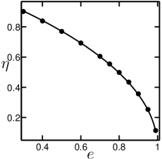
(a) (b)

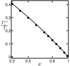
Figure 12: Comparisons of (a) shear-plane temperature-anisotropy $\eta$ and (b) the excess temperature $T^{ex}_{z}/T\equiv 2\lambda^{2}$ in uniform shear flow of a granular gas ($St=\infty$): MD simulation (symbols) and theory [solid line, Saha & Alam (2016)]. The particle volume fraction is $\nu=0.01$ and the number of particles is $N=1000$ in simulations.

Figures 13(a) and  13(b) compare the MD simulation data (symbols) for ${\mathcal{N}}_{1}$ and ${\mathcal{N}}_{2}$, respectively, with theory; the AME predictions, denoted by solid lines, are calculated from (59) and (60) by setting $St\to\infty$ (Saha & Alam, 2016), and the corresponding GME-predictions (Appendix E) are denoted by dashed lines. In addition, the dot-dashed line in each panel represents the super-Burnett-order solution of Sela & Goldhirsch (1998), obtained from the Chapman-Enskog expansion of inelastic Boltzmann equation. It is clear that both GME and AME theories predict almost the same value of ${\mathcal{N}}_{1}$ for a range of restitution coefficient $e\in(0.3,1)$, but the GME-prediction for ${\mathcal{N}}_{2}$ is consistently lower than that of AME and can be off by a factor of $3$ at $e=0.3$. On the other hand, the AME-predictions for both ${\mathcal{N}}_{1}$ and ${\mathcal{N}}_{2}$ are comparable to those of Chapman-Enskog solution for $e\geq 0.8$, but the latter becomes increasingly inaccurate for $e<0.8$. Therefore, the quantitative predictions of the AME for two normal stress differences are better than those of GME and Chapman-Enskog solution – this overall conclusion holds for both gas-solid and dry granular suspensions of inelastic particles.

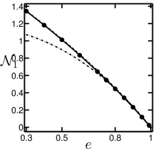
(a) (b)

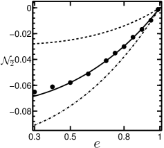
Figure 13: Comparisons of (a) ${\mathcal{N}}_{1}$ and (b) ${\mathcal{N}}_{2}$ in uniform shear flow of a granular gas ($St=\infty$): (i) MD simulation (symbols), (ii) present theory [solid lines, Saha & Alam (2016)] and (iii) the standard Grad’s moment theory (dashed line). The dot-dash line in each panel represent the super-Burnett-order Chapman-Enskog solution of Sela & Goldhirsch (1998), see Appendix F. Parameter values as in figure 12.

6 Summary and Conclusion

The rheology of a dilute gas-solid suspension, consisting of inelastic spheres suspended in a Newtonian fluid, undergoing simple shear flow is analysed, with the effect of the gas-phase being modelled via a Stokesian drag force. The pertinent inelastic Boltzmann equation is solved using an anisotropic Gaussian as the single particle distribution function which is known to be appropriate for a sheared system. The resulting hydrodynamic model for the particle-phase consists of a 10-moment system $(\rho,{\boldsymbol{u}},{\mathsfb M})$ of density ($\rho$), hydrodynamic velocity ($\bf u$) and the second-moment (${\mathsfb M}=\langle{\boldsymbol{C}}{\boldsymbol{C}}\rangle$) of fluctuation/peculiar velocity. One focus of the present work has been to analyse the anisotropy of ${\mathsfb M}$ in the simple shear flow of a dilute gas-solid suspension and subsequently tie and explain the rheological quantities in terms of them.

The seond-moment tensor has been characterized by three parameters: (i) the non-coaxiality angle ($\phi$, the angle between the principal eigen-direction of ${\mathsfb M}$ and the shear tensor ${\mathsfb D}$), (ii) the shear-plane temperature-anisotropy ($\eta$, the difference between the principal eigenvalues of ${\mathsfb M}$ on the shear plane, $\eta\propto T_{x}-T_{y}$, where $T_{i}$ is the granular temperature along $i$-th direction) and (iii) the excess temperature ($\lambda^{2}\propto T-T_{z}$) along the vorticity direction; the first two [$\phi$ and $\eta$] are dubbed ‘shear-plane’ anisotropies and the last-one ($\lambda^{2}$) is dubbed vorticity-plane anisotropy. The closed-form expressions for three anisotropy parameters ($\phi$, $\eta$, $\lambda^{2}$) and the granular temperature ($T$) have been obtained as functions of the Stokes number ($St$), the mean density ($\nu$) and the restitution coefficient ($e$) by solving the second-moment balance equation; these are used to obtain analytical expressions for the particle-phase viscosity and two normal-stress differences. Scaling relations have been obtained in the limits of small and large $St$ as well as small inelasticity $(1-e)$.

Static multiple states of high and low temperatures are found when the Stokes number is small enough, thereby recovering the original “ignited” ($I$) and “quenched” ($Q$) states of Tsao & Koch (1995) – the role of inelasticity on these states has been examined. The high-temperature ignited state, in which the randomness of the particle motion is high giving rise to a large value of granular temperature ($T$), exists above some minimum Stokes number $(St_{c_{1}})$ whose value increases with increasing $e$. In contrast, the low-temperature quenched state, in which most of the particles in the system follow the local fluid velocity, appears below a critical value of Stokes number $(St_{c_{2}})$ which is a decreasing function of both $e$ and $\nu$. Both these Stokes numbers ($St_{c_{1}}$ and $St_{c_{2}}$) have been determined analytically as functions of $\nu$ and $e$, and the regions of co-existence of two states (quenched and ignited) along with the transition regimes have been identified in a three-dimensional ($St,e,\nu$) phase diagram.

The effect of inelasticity is found to reduce the particle-phase viscosity on both ignited and quenched states, with shear-thickening behaviour (increasing viscosity with increasing shear rate) being found in both states. At any $e$, the shear-viscosity undergoes a discontinuous jump with increasing $St$ at “$Q\rightarrow I$” transition, which can be interpreted as “discontinuous shear thickening” (DST). The two normal stress differences also undergo similar first-order jump-transitions: (i) ${\mathcal{N}}_{1}$ from large to small positive values and (ii) ${\mathcal{N}}_{2}$ from positive to negative values. The sign-change of ${\mathcal{N}}_{2}$ (figure 10) has been identified with the system being making a “$Q\leftrightarrow I$” transition. The origin of this sign-change has been tied to a competition between (i) the excess temperature ($T_{z}^{ex}\propto 3\lambda^{2}$) and (ii) the shear-plane anisotropies ($\eta\sin{2\phi}\equiv{\mathcal{N}}_{1}/2$) of the second-moment tensor: while the former dominates over the latter in the quenched state, the latter dominates in the ignited state, resulting in the sign-change of ${\mathcal{N}}_{2}$ at some finite value of $St$. For both granular and gas-solid suspensions, the excess temperature along the vorticity direction is responsible for the origin of ${\mathcal{N}}_{2}\neq 0$, while the temperature anisotropy $\eta$ and the non-coaxiality angle $\phi$ are responsible for ${\mathcal{N}}_{1}\neq 0$.

The comparative analyses in figures 2, 10, 11, 12 and 13 can be summarized as follows: the moment expansion about an anisotropic-Maxwellian (AME) yields accurate transport coefficients (shear viscosity and normal stress differences) for dissipative particles ($e<1$) in both small and large Stokes number limits, representative of gas-solid and dry granular suspensions, respectively. The standard Grad’s moment-expansion (GME) significantly under-predicts the value of the second normal stress difference ${\mathcal{N}}_{2}$, although it is comparable with AME with respect to ${\mathcal{N}}_{1}$ up-to a restitution coefficient of $e=0.5$. On the other hand, the latter theory (GME) also over-predicts the shear viscosity ($\mu\propto\sqrt{T}$, viz. figure 2) of small-$St$ suspensions even for moderately dissipative ($e=0.8$) particles; the mismatch between GME and simulation increases with decreasing $e$. Based on the present work we conclude that the superior predictive ability of the AME theory for hydrodynamics and rheology of ‘dry’ ($St\to\infty$) sheared granular gases (Saha & Alam, 2014, 2016) carries over to small-$St$ gas-solid suspensions of highly inelastic particles.

It would be interesting to check the applicability of this theory to dense gas-solid suspensions of inelastic particles (with frictional interactions) which can be taken up in future. The present work can also be extended to include a ‘non-linear’ drag law (dependence on particle Reynolds number) by modifying (6) via well-known empirical correlations. Lastly, the anisotropies ($\phi,\eta,\lambda^{2}$) of the second-moment tensor should be measured from simulations of finite-$St$ suspensions so that one-to-one comparisons with theory can be made in this regard.

Appendix A Analysis in the ignited state for elastic hard-spheres

For a gas-solid suspension of elastic hard-spheres ($e=1$), the collisional source of second-moment in the ignited state is given by

$$\aleph_{\alpha\beta} = \frac{-24\rho_{p}\nu^{2}}{\sigma\pi^{\frac{3}{2}}}\int(k_{\alpha}j_{\beta}+k_{\beta}j_{\alpha})({\textbf{\emph{k}}}\cdot{{\mathsfb M}}\cdot{\textbf{\emph{j}}})({\textbf{\emph{k}}}\cdot{{\mathsfb M}}\cdot{\textbf{\emph{k}}})^{\frac{1}{2}}d{\boldsymbol{k}}$$ (69)

$$= -\frac{32\rho_{p}\nu^{2}T^{3/2}}{35\sigma\sqrt{\pi}}\times$$

$$\left[\begin{array}[]{ccc}\eta^{2}+21\lambda^{2}+21\eta\sin 2\phi&-21\eta\cos 2\phi&0\\ -21\eta\cos 2\phi&\eta^{2}+21\lambda^{2}-21\eta\sin 2\phi&0\\ 0&0&-2(\eta^{2}+21\lambda^{2})\end{array}\right],$$

which is a function of $\nu$,$T$, $\eta$, $\phi$ and $\lambda^{2}$.

Four independent equations of second-moment balance,

$$P_{\delta\beta}u_{\alpha,\delta}+P_{\delta\alpha}u_{\beta,\delta}+\frac{2\gamma}{St}P_{\alpha\beta}=\aleph_{\alpha\beta},$$ (70)

can be rearranged to yield a quartic-order equation,

$$\omega^{2}\Big{[}12096St^{2}\omega^{2}+\left(10260St-420St^{3}\right)\omega+3225-175St^{2}\Big{]}=0,$$ (71)

where $\omega$ is the rescaled temperature

$$\omega=\frac{\nu}{\sqrt{\pi}}\frac{\sqrt{T}}{(\dot{\gamma}\sigma/2)}.$$ (72)

In the following, the temperature has been made dimensionless by dividing it by $(\dot{\gamma}\sigma/2)^{2}$. Three distinct solutions of (71) are

$$\sqrt{T_{is}} = \frac{5\pi^{\frac{1}{2}}}{144}\frac{St}{\nu}\Omega(St),$$ (73)

$$\sqrt{T_{us}} = \frac{5\pi^{\frac{1}{2}}}{144}\frac{St}{\nu}\Big{[}\frac{7St^{2}-171-\sqrt{49St^{4}-42St^{2}-14103}}{14St^{2}}\Big{]},$$ (74)

$$T_{qs} = 0,$$ (75)

with $T_{is}>T_{us}>T_{qs}$, where

$$\Omega(St)=\Big{[}\frac{7St^{2}-171+\sqrt{49St^{4}-42St^{2}-14103}}{14St^{2}}\Big{]}\equiv\frac{144}{5}\omega_{is}St^{-1}.$$ (76)

In the above expressions, $T_{qs}$ corresponds to the quenched state temperature, $T_{us}$ corresponds to an unstable temperature and $T_{is}$ corresponds to the temperature in the ignited state. It is clear from (74) that a positive value for $T_{us}$ requires the following condition on the Stokes number:

$$7St^{2}-171\geqslant 0,\qquad\Rightarrow\quad St\geqslant\sqrt{\frac{171}{7}}\approx 4.9425\equiv St_{c_{1}}.$$ (77)

Therefore, $St$ must be greater than or equal to $St_{c_{1}}$, and (77) provides a lower bound on $St$ for the existence of the ignited state in a dilute sheared gas-solid suspension.

The remaining equations of (70) can be solved to yield solutions for $\eta^{2}$ and $\lambda^{2}$ in the ignited state:

$$\left.\begin{array}[]{lcl}\eta^{2}&=&\frac{(9+\Omega St^{2})}{4\left(1+\frac{29}{84}\Omega St^{2}+\frac{1}{36}\Omega^{2}St^{4}\right)}\\ \lambda^{2}&=&\frac{(7+\Omega St^{2})}{14\left(1+\frac{29}{84}\Omega St^{2}+\frac{1}{36}\Omega^{2}St^{4}\right)}\end{array}\right\};$$ (78)

the solution for the non-coaxilality angle is

$$\sin(2\phi)=\frac{\eta}{1+\lambda^{2}}.$$ (79)

Therefore, the normal stress differences in the ignited state are given by

$$\mathcal{N}_{1} = \frac{15}{5+24St\omega}\equiv\frac{18}{6+\Omega St^{2}},$$ (80)

$$-\mathcal{N}_{2} = \frac{270St\omega(5+16St\omega)}{(5+24St\omega)(175+1740St\omega+4032St^{2}\omega^{2})}.$$ (81)

In the ignited state, the expression for the shear viscosity of the particle phase is

$$\mu=-P_{xy}/\dot{\gamma}=\mu_{N}\Omega(St),$$ (82)

where

$$\mu_{N}=\frac{5\sqrt{\pi}}{96}\rho_{p}\sigma\sqrt{T}$$ (83)

is the Newtonian viscosity of a dilute gas. Therefore, $\Omega(St)$ [(76)] is a measure of the deviation of particle-phase viscosity from the Newtonian viscosity of a dilute hard-sphere gas.

Appendix B Coefficients $a_{i}$

Explicit expressions of the individual coefficients $a_{i}$ appearing in (39) are given by:

$$a_{10} = 86416243200(3-e)^{4}(1-e)^{3}(1+e)^{7}\pi St^{6}\nu^{7},$$ (84)

$$a_{9} = 28805414400(3-e)^{3}(1-e)^{2}(1+e)^{6}(19-13e)\pi^{(3/2)}St^{5}\nu^{6},$$ (85)

$$a_{8} = 28576800(3-e)^{2}(1-e)(1+e)^{5}\pi^{2}St^{4}\nu^{5}\Big{(}252(197-278e+93e^{2})$$ (86)

$$\qquad\qquad\qquad\qquad\qquad\qquad+5(1747-1438e+363e^{2})St^{2}\Big{)},$$

$$a_{7} = 3810240(3-e)(1+e)^{4}\sqrt{\pi}St^{3}\nu^{4}\Big{(}2100(1-e)(241-284e+79e^{2})\pi^{2}$$ (87)

$$\qquad\qquad\qquad\qquad+25(12607-19952e+10099e^{2}-1746e^{3})\pi^{2}St^{2}$$

$$\qquad\qquad\qquad\qquad\qquad\qquad-3456(3-e)^{3}(1-e)^{2}(1+e)^{4}St^{3}\nu^{3}\Big{)},$$

$$a_{6} = 79380(1+e)^{3}\pi St^{2}\nu^{3}\Big{(}21000(1-e)(871-854e+199e^{2})\pi^{2}$$ (88)

$$\qquad\qquad\qquad\qquad+500(56617-78677e+35629e^{2}-5361e^{3})\pi^{2}St^{2}$$

$$\qquad\qquad\qquad\qquad-125(1691+539e-1223e^{2}+337e^{3})\pi^{2}St^{4}$$

$$\qquad\qquad\qquad\qquad-27648(3-e)^{3}(1-e)(1+e)^{4}(29-23e)St^{3}\nu^{3}\Big{)},$$

$$a_{5} = 18900(1+e)^{2}\pi^{(3/2)}St\nu^{2}\Big{(}441000(1-e)(23-11e)\pi^{2}$$ (89)

$$+10500(3437-3093e+688e^{2})\pi^{2}St^{2}-875(477+442e-247e^{2})\pi^{2}St^{4}$$

$$\qquad\qquad-580608(3-e)^{2}(1-e)(1+e)^{4}(11-7e)St^{3}\nu^{3}$$

$$\qquad\qquad-1152(3-e)^{2}(1+e)^{4}(991-934e+279e^{2})St^{5}\nu^{3}\Big{)},$$

$$a_{4} = 63(1+e)\nu\Big{(}165375000(1-e)\pi^{4}+656250(2437-1069e)\pi^{4}St^{2}$$ (90)

$$-109375(107+193e)\pi^{4}St^{4}-48384000(3-e)(1-e)(1+e)^{4}(37-19e)\pi^{2}St^{3}\nu^{3}$$

$$-288000(3-e)(1+e)^{4}(3917-3368e+843e^{2})\pi^{2}St^{5}\nu^{3}$$

$$-3024000(3-e)^{3}(1+e)^{4}\pi^{3}St^{6}\nu^{3}+7962624(3-e)^{4}(1-e)(1+e)^{8}St^{6}\nu^{6}\Big{)},$$

$$a_{3} = 2520\sqrt{\pi}St\Big{(}2296875\pi^{4}-504000(1-e)(1+e)^{4}(41-17e)\pi^{2}St\nu^{3}$$ (91)

$$-6000(1+e)^{4}(5617-4438e+933e^{2})\pi^{2}St^{3}\nu^{3}-189000(3-e)^{2}(1+e)^{4}\pi^{3}St^{4}\nu^{3}$$

$$-1000(1+e)^{4}(1203-1002e+247e^{2})\pi^{2}St^{5}\nu^{3}$$

$$+663552(3-e)^{3}(1-e)(1+e)^{8}St^{4}\nu^{6}\Big{)},$$

$$a_{2} = -2400(1+e)^{3}\pi St\nu^{2}\Big{(}1323000(1-e)\pi^{2}+15750(383-151e)\pi^{2}St^{2}$$ (92)

$$+165375(3-e)\pi^{3}St^{3}+875(789-305e)\pi^{2}St^{4}$$

$$-870912(3-e)^{2}(1-e)(1+e)^{4}St^{3}\nu^{3}-1728(3-e)^{2}(1+e)^{4}(47-39e)St^{5}\nu^{3}\Big{)},$$

$$a_{1} = -2000(1+e)^{2}\pi^{(3/2)}St^{2}\nu\Big{(}441000\pi^{2}+55125\pi^{3}St+98000\pi^{2}St^{2}$$ (93)

$$-580608(3-e)(1-e)(1+e)^{4}St\nu^{3}-3456(3-e)(1+e)^{4}(47-39e)St^{3}\nu^{3}\Big{)},$$

$$a_{0} = 1440000(1+e)^{5}\pi^{2}St^{2}(4+St^{2})\nu^{3}\Big{(}42(1-e)+(13-9e)St^{2}\Big{)}.$$ (94)

Appendix C Ordering analysis to determine three temperatures

We will solve (39) analytically in the asymptotic limit $\nu\ll 1$, $St\gg 1$, and $St^{3}\nu\ll 1$ (Tsao & Koch, 1995), and three feasible solutions have been found as described below.

C.1 Temperature in the quenched state

For $\xi\sim O(St^{3/2}\sqrt{\nu})$, the leading order term in (39) is $O(St^{\frac{11}{2}}\nu^{\frac{3}{2}})$ and consequently we have

$$a_{3}\xi^{3}+a_{1}\xi=0,$$ (95)

where

$$a_{3}=5788125000\upi^{\frac{9}{2}}St,\qquad a_{1}=-196000000\upi^{\frac{7}{2}}(1+e)^{2}St^{4}\nu.$$ (96)

The solution at this level of approximation is

$$T_{qs}=\xi^{2}=\frac{32(1+e)^{2}}{945\upi}St^{3}\nu,$$ (97)

which corresponds to the temperature in the quenched state. Note that the quenched temperature increases with increasing both $St$ and $\nu$.

C.2 Unstable temperature

When $\xi\sim O(St^{3}\nu)^{-1}$, the highest-order term in (39) is $O(1/St^{8}\nu^{3})$, and on neglecting terms smaller than this, we have at leading order

$$a_{4}\xi^{4}+a_{3}\xi^{3}=0,$$ (98)

where

$$a_{4}=-6890625(1+e)(107+193e)\upi^{4}St^{4}\nu,\qquad a_{3}=5788125000\upi^{\frac{9}{2}}St.$$ (99)

Therefore, we have

$$\sqrt{T_{us}}=\xi=\frac{840\sqrt{\upi}}{(1+e)(107+193e)}\left(\frac{1}{St^{3}\nu}\right),$$ (100)

This is the temperature of an intermediate state which is unstable – note that $T_{us}$ decreases with increasing $St$ and $\nu$.

C.3 Temperature in the ignited state

In the asymptotic limit of $\xi\sim O(St/\nu)$, the leading order term of $a_{i}\xi^{i}\;i=0(1)11$ is $O(St^{12}/\nu^{3})$ and consequently we have from (39)

$$a_{7}\xi^{7}+a_{6}\xi^{6}=0,$$ (101)

where

$$\left.\begin{array}[]{lcl}a_{7}&=&95256000(3-e)(1+e)^{4}(12607-19952e+10099e^{2}-1746e^{3})\upi^{\frac{5}{2}}St^{5}\nu^{4},\\ a_{6}&=&-9922500(1+e)^{3}(1691+539e-1223e^{2}+337e^{3})\upi^{3}St^{6}\nu^{3}.\end{array}\right\}.$$ (102)

Therefore, the temperature at this order of approximation is

$$\sqrt{T_{is}}=\xi=\frac{5(1691+539e-1223e^{2}+337e^{3})\sqrt{\upi}}{48(3-e)(1+e)(12607-19952e+10099e^{2}-1746e^{3})}\left(\frac{St}{\nu}\right),$$ (103)

which corresponds to the temperature in the ignited state. While $T_{is}$ increases with increasing $St$, it deceases with increasing the particle volume fraction $\nu$.

Appendix D Analytical determination of limit-points $St_{c_{1}}$ and $St_{c_{2}}$

At the critical/limit points, two solution branches of (39) corresponding to two different states [(i) quenched $(T_{qs})$ and unstable $(T_{us})$ states and (ii) unstable $(T_{us})$ and ignited $(T_{is})$ states] meet and consequently we have saddle-node bifurcations from one stable state to another. Therefore, these limit points correspond to the double roots of (39) at which the following conditions must be satisfied:

$$\mathcal{G}(\xi_{c})=0\quad\mbox{and}\quad\mathcal{G}^{\prime}(\xi_{c})=0.$$ (104)

D.1 Determining $St_{c_{1}}$: discontinuous transition from “ignited” to “quenched” states

The critical Stokes number, $St_{c_{1}}$, for the transition from the ignited to quenched states corresponds to the limit point at which the temperatures corresponding to the ignited ($T_{is}$) and unstable ($T_{us}$) branches overlap with each other. Considering $\xi\sim O(\nu St)^{-1}\gg 1$, and retaining the highest-order terms, (39) reduces to

$$\mathcal{G} \approx a_{7}\xi^{7}+a_{6}\xi^{6}+a_{5}\xi^{5}+a_{4}\xi^{4}+a_{3}\xi^{3}=0=a_{7}\xi^{4}+a_{6}\xi^{3}+a_{5}\xi^{2}+a_{4}\xi+a_{3},$$ (105)

$${\rm and} 4a_{7}\xi^{3}+3a_{6}\xi^{2}+2a_{5}\xi+a_{4}=0,$$ (106)

where

$$\left.\begin{array}[]{rcl}a_{7}&=&95256000(3-e)(1+e)^{4}(12607-19952e+10099e^{2}-1746e^{3})\pi^{\frac{5}{2}}St^{5}\nu^{4},\\ a_{6}&=&9922500(1+e)^{3}\pi^{3}St^{4}\Big{(}4(56617-78677e+35629e^{2}-5361e^{3})\\ &&\qquad\qquad\qquad\qquad\qquad\qquad-(1691+539e-1223e^{2}+337e^{3})St^{2}\Big{)}\nu^{3},\\ a_{5}&=&16537500(1+e)^{2}\pi^{\frac{7}{2}}St^{3}\Big{(}12(3437-3093e+688e^{2})\\ &&\qquad\qquad\qquad\qquad\qquad\qquad-(477+442e-247e^{2})St^{2}\Big{)}\nu^{2},\\ a_{4}&=&6890625(1+e)\pi^{4}St^{2}(6(2437-1069e)-(107+193e)St^{2})\nu,\\ a_{3}&=&5788125000\pi^{\frac{9}{2}}St.\end{array}\right\}$$ (107)

Using the condition of equal roots of a fourth-degree polynomial (105), we obtain an expression for the critical Stokes number for the “ignited-to-unstable” transition:

$$St_{c_{1}}\approx 9.9-4.91e.$$ (108)

While decreasing the Stokes number along the ignited-state branch (see figure 2), the system jumps from the ignited to the quenched state at $St<St_{c_{1}}$ for all $\nu<\nu^{l}_{us}$ (3.8). Therefore, (108) represents the minimum/critical Stokes number below which (39) admits the unique “quenched” state solution.

D.2 Determining $St_{c_{2}}$: discontinuous transition from “quenched” to “ignited” state

The limit point corresponding to the overlap of the quenched and unstable branches of the system is denoted by the Stokes number $St_{c_{2}}$ at which the temperatures associated with the quenched ($T_{qs}$) and unstable ($T_{us}$) states coincide – above this critical value of Stokes number the quenched state ceases to exist. Mathematically, $St_{c_{2}}$ is the point of the double root $T_{is}=T_{us}$ of (39). above which there exists only one feasible solution $T_{is}$ (corresponding to the ignited state) and the system jumps from the quenched state into the ignited state At this order of approximation $\xi\sim O(1)$ and the highest order terms are of the orders of $\nu St^{4}$ and $St$. Therefore on neglecting the terms of $O(St^{4}\nu^{2})$ and using the statement of $T_{is}=T_{us}$, we have from (39)

$$\mathcal{G}(\xi_{c}) \approx a_{4}\xi^{4}+a_{3}\xi^{3}+a_{1}\xi=0=a_{4}\xi^{3}+a_{3}\xi^{2}+a_{1},$$ (109)

$${\rm and}\quad\mathcal{G}^{\prime}(\xi_{c}) \approx 3a_{4}\xi^{2}+2a_{3}\xi=0,$$ (110)

where

$$\left.\begin{array}[]{rcl}a_{4}&=&-6890625(1+e)(107+193e)\pi^{4}St^{4}\nu,\\ a_{3}&=&5788125000\pi^{\frac{9}{2}}St,\\ a_{1}&=&-196000000(1+e)^{2}\pi^{\frac{7}{2}}St^{4}\nu.\end{array}\right\}$$ (111)

It follows from (110) that

$$\xi_{c}=\frac{-2a_{3}}{3a_{4}}=\frac{560\sqrt{\pi}}{(1+e)(170+193e)St^{3}\nu}.$$ (112)

On substituting (112) into (109) we obtain the critical-surface

$$St_{c_{2}}^{3}\nu_{c}=\Bigg{(}\frac{3087000\pi^{2}}{(1+e)^{4}(107+193e)^{2}}\Bigg{)}^{\frac{1}{3}},$$ (113)

above which only the ignited state exists.

Appendix E Grad’s moment expansion (GME) for inelastic gas-solid suspension

The standard Grad’s moment expansion (GME) in terms of a truncated Hermite series around the Maxwellian (Grad, 1949) has been employed by many researchers (Herdegen & Hess, 1982; Tsao & Koch, 1995; Chamorro, Reyes & Garzo, 2015) to analyse the Boltzmann equation for a “sheared” hard-sphere gas as well as gas-solid suspensions.

• Herdegen & Hess (1982)$\Rightarrow$ $e=1,\;St=\infty$  (Dilute gas of elastic hard-spheres)

• Tsao & Koch (1995)$\Rightarrow$ $e=1,\;St$ finite  (Suspension of elastic hard-spheres)

• Chamorro, Reyes & Garzo (2015)$\Rightarrow$ $e\neq 1,\;St$ finite  (Suspension of inelastic hard-spheres)

For the case of a dilute gas-solid suspension of “inelastic” hard-spheres, the collisional production term of the second moment has been evaluated as:

$$\aleph_{\alpha\beta} = -\frac{8\rho_{p}\nu^{2}(1-e^{2})T^{\frac{3}{2}}}{\sqrt{\pi}\sigma}\delta_{\alpha\beta}-\frac{24\nu(1+e)(3-e)T^{\frac{1}{2}}}{5\sqrt{\pi}\sigma}P_{\langle\alpha\beta\rangle}$$ (114)

$$+\frac{(1+e)}{35\sqrt{\pi}\sigma\rho_{p}T^{\frac{1}{2}}}\underline{\Big{\{}(5+3e)P_{\langle kl\rangle}P_{\langle kl\rangle}\delta_{\alpha\beta}+12(e-3)P_{\langle\alpha l\rangle}P_{\langle l\beta\rangle}\Big{\}}},$$

where the underlined terms represent the quadratic nonlinearity in the pressure deviator $P_{\langle\alpha\beta\rangle}=P_{\alpha\beta}-p\delta_{\alpha\beta}$, with $p=P_{\alpha\alpha}/3$; $\rho_{p}=m/(\pi\sigma^{3}/6)$ is the intrinsic/material density of particles, $\nu$ is the particle volume fraction and $e$ is the restitution coefficient. In fact, the second normal-stress difference is zero (${\mathcal{N}}_{2}=0$) in the absence of the underlined non-linear terms in (114), see the proof at the end of this appendix.

Defining the non-dimensional quantities as

$$P^{*}=\frac{P}{\rho_{p}\nu(\dot{\gamma}\sigma/2)^{2}},\qquad T^{*}=\frac{T}{(\dot{\gamma}\sigma/2)^{2}},\qquad\aleph^{*}=\frac{\aleph}{\rho_{p}\nu{\dot{\gamma}}^{3}(\sigma/2)^{2}},$$ (115)

and on omitting the $*$ signs, for convenience, the dimensionless second-moment balance for steady homogeneous shear flow,

$$P_{\delta\beta}u_{\alpha,\delta}+P_{\delta\alpha}u_{\beta,\delta}+\frac{2}{St}P_{\alpha\beta}=\aleph_{\alpha\beta},$$ (116)

can be written in component form as follows:

$$(1+e)(5+3e)\Big{(}P_{\langle xx\rangle}^{2}+P_{\langle yy\rangle}^{2}+P_{\langle zz\rangle}^{2}+2P_{xy}^{2}\Big{)}-12(1+e)(3-e)\Big{(}P_{\langle xx\rangle}^{2}+P_{xy}^{2}\Big{)}$$

$$\qquad\qquad-280(1-e^{2})T^{2}-168(1+e)(3-e)TP_{\langle xx\rangle}-\frac{140\sqrt{\pi}\sqrt{T}P_{xy}}{\nu}$$

$$\hskip 199.16928pt-\frac{140\sqrt{\pi}\sqrt{T}}{St\nu}(T+P_{\langle xx\rangle})=0,$$ (117)

$$(1+e)(5+3e)\Big{(}P_{\langle xx\rangle}^{2}+P_{\langle yy\rangle}^{2}+P_{\langle zz\rangle}^{2}+2P_{xy}^{2}\Big{)}-12(1+e)(3-e)\Big{(}P_{\langle yy\rangle}^{2}+P_{xy}^{2}\Big{)}$$

$$\qquad-280(1-e^{2})T^{2}-168(1+e)(3-e)TP_{\langle yy\rangle}-\frac{140\sqrt{\pi}\sqrt{T}}{St\nu}(T+P_{\langle yy\rangle})=0,$$ (118)

$$(1+e)(5+3e)\Big{(}P_{\langle xx\rangle}^{2}+P_{\langle yy\rangle}^{2}+P_{\langle zz\rangle}^{2}+2P_{xy}^{2}\Big{)}-12(1+e)(3-e)P_{\langle zz\rangle}^{2}$$

$$\qquad-280(1-e^{2})T^{2}-168(1+e)(3-e)TP_{\langle zz\rangle}-\frac{140\sqrt{\pi}\sqrt{T}}{St\nu}(T+P_{\langle zz\rangle})=0,$$ (119)

$$12(1+e)(3-e)P_{xy}P_{\langle zz\rangle}-168(1+e)(3-e)TP_{xy}-\frac{70\sqrt{\pi}\sqrt{T}}{\nu}(T+P_{\langle yy\rangle})$$

$$\hskip 227.62204pt-\frac{140\sqrt{\pi}T^{\frac{1}{2}}}{St\nu}P_{xy}=0,$$ (120)

along with constraint $\widehat{P}_{\alpha\alpha}=0$. These equations have been solved numerically for specified values of $e$, $St$ and $\nu$ to yield $T$, $P_{\langle\alpha\alpha\rangle}$ and $P_{xy}$; two normal stress differences ${\mathcal{N}}_{1}$ and ${\mathcal{N}}_{2}$ can be expressed in terms of $P_{\langle\alpha\alpha\rangle}$. These are dubbed “GME” solutions and their comparisons with the present theory (§4) based on anisotropic-Maxwellian expansion (AME) are shown in figures  10, 11 and 13, as discussed in §5.1 and §5.2.

Theorem 1

The source term is uniquely decomposed as $\aleph_{\alpha\beta}=\left(\frac{1}{3}\aleph_{\gamma\gamma}\right)\delta_{\alpha\beta}+\aleph_{\langle\alpha\beta\rangle}$. If $\aleph_{\langle\alpha\beta\rangle}=BP_{\langle\alpha\beta\rangle}$, then ${\mathcal{N}}_{2}=0$.

Proof E.2.

For the case of homogeneous shear $u_{x}=\dot{\gamma}y$, $u_{y}=0$, $u_{z}=0$; the balance of second moment for a granular gas is

$${\rm P}_{\delta\beta}{\rm u}_{\alpha,\delta}+{\rm P}_{\delta\alpha}{\rm u}_{\beta,\delta}=\aleph_{\alpha\beta}.$$ (121)

Now, upon substituting $\alpha=2$, $\beta=2$ and $\alpha=3$, $\beta=3$ we have

$$\aleph_{22}=0=\aleph_{33}.$$ (122)

From ${P}_{ij}=p\delta_{ij}+{P}_{\langle ij\rangle}$, we can write

$${\mathcal{N}}_{2}=\left({P}_{\langle 22\rangle}-{P}_{\langle 33\rangle}\right)=B^{-1}\left({\aleph}_{\langle 22\rangle}-{\aleph}_{\langle 33\rangle}\right)=0.$$ (123)

Of course, (123) is in contradiction with (i) the nonlinear expression (114) obtained from the standard Grad-moment expansion as well as with (ii) our choice of anisotropic Maxwellian distribution function, both yielding ${\mathcal{N}}_{2}\neq 0$.

References

- Alam & Luding (2005) Alam, M. & Luding, S. 2005 Non-Newtonian granular fluid: Simulation and theory. In Powders & Grains (Editors: R. Garcia-Rojo, H. J. Herrmann and S. McNamara), pp. 1141-1144, A. A. Balkema.
- Alam & Saha (2017) Alam, M. & Saha, S. 2017 Normal stress differences and beyond-Navier-Stokes hydrodynamics. EPJ Conf. Proc. 140, (Powders and Grains 2017)
- Anderson & Jackson (1968) Anderson, T. B. & Jackson, R. 1968 A fluid mechanical description of fluidized beds: equations of motion. Ind. Eng. Chem. Fundam. 6, 527-539.
- Araki (1988) Araki, S. 1988 The dynamics of particle disks: II. Effects of spin degrees of freedom. Icarus 76, 182-198.
- Araki & Tremaine (1986) Araki, S. & Tremaine, S. 1986 The dynamics of dense particle disks. Icarus 65, 83-109.
- Boyer, Pouliquen & Guazzelli (2011) Boyer, F., Pouliquen, O. & Guazzelli, E. 2011 Dense suspensions in rotating-rod flows: normal stresses and particle migration. J. Fluid Mech. 686, 5-25.
- Brey et al. (1998) Brey, J. J., Dufty, J. W., Kim, C. S. & Santos, A. 1998 Hydrodynamics for granular flow at low density. Phys. Rev. E 58, 4638?4653.
- Brilliantov & Pöschel (2004) Brilliantov, N. V. & Pöschel, T. 2004 Kinetic Theory of Granular Gases. Oxford Univ. Press.
- Brown & Jaeger (2014) Brown, E. & Jaeger, H. M. 2014 Shear thickening in concentrated suspensions. Rep. Prog. Phys., 77, 046602.
- Buyevich (1971) Buyevich, Y. A. 1971 Statistical hydrodynamics of disperse systems, Part 1. physical background and general equations. J. Fluid Mech. 49, 489-507.
- Callen (1985) Callen, H. B. 1985 Thermodynamics and an introduction to Thermostatics. John Wiley Sons
- Campbell (1990) Campbell, C. S. 1990 Rapid granular flows. Annu. Rev. Fluid Mech. 22, 57-90.