trackr: A Framework for Enhancing Discoverability and Reproducibility of Data Visualizations and Other Artifacts in R

Abstract

Research is an incremental, iterative process, with new results relying and building upon previous ones. Scientists need to find, retrieve, understand, and verify results in order to confidently extend them, even when the results are their own. We present the trackr framework for organizing, automatically annotating, discovering, and retrieving results. We identify sources of automatically extractable metadata for computational results, and we define an extensible system for organizing, annotating, and searching for results based on these and other metadata. We present an open-source implementation of these concepts for plots, computational artifacts, and woven dynamic reports generated in the R statistical computing language.

Keywords: metadata, computing, provenance, publishing

1 Introduction

Research is an incremental, iterative process, with new results relying and building upon previous ones. Scientists need to find, retrieve, understand, and verify results in order to confidently extend them, even when the results are their own. Understanding an existing result requires knowing how it was generated (Rossini and Leisch 2003; Becker 2014). Associating a result with the set of actions (Lee and Grinstein 1995) or code (Claerbout and Karrenbach 1992; Buckheit and Donoho 1995; Leisch 2002) that generated it enhances the understandability and reproducibility of the result. Further associating a result with information about the input data and the software involved provides even stronger guarantees of reproducibility (Gentleman and Temple Lang 2004; Stodden et al. 2015). Researchers must be aware of a result in order to extend it, so the tracking, organization, and discoverability of results is key to their incorporation into a larger body of scientific work. The ability of a scientist to find and retrieve an existing result from within a body of results depends on how well the result is annotated with metadata that enable its discovery and differentiate it from other results (Figshare Support Team 2016).

Standardized tracking, organization, and annotation of results serves different purposes when leveraged at different organizational scales. Individual analysts often generate dozens of visualizations and other artifacts during a single analysis. They then retrieve particular results as needed — e.g., when presenting in a group meeting, preparing a manuscript, or reviewing past work. When their results are organized and stored in standard ways, locating and retrieving the correct artifact is easier and less error-prone (Schwab et al. 2000). Searching for a result based on metadata annotations, for example the datasets and variables used, plot title, statistical model type and specification, etc., is generally easier still and more efficient than manually locating an image file or serialized result on the file system — particularly as the number of results and the time since their creation grow. Beyond locating individual results, metadata can identify groups of related results, such as those involving a certain variable or data subset. This grants the analyst a more holistic, retrospective view of their analysis, potentially leading to new insights derived from the synergy of many individual results.

Systematic tracking of results provides additional benefits to research teams and the broader scientific community at large. Tracking artifacts in a standardized way across multiple analysts, projects, and research efforts facilitates the creation and effective use of a body of institutional or communal knowledge. This increases an organization’s effectiveness by reducing duplication of work, helping identify connections between related or synergistic work, and increasing the impact of results. Sharing results is necessary for collaboration between analysts and subject-material experts. For these and other reasons, standalone publication of datasets, plots (Plotly Technologies Inc. 2013; RStudio Inc. ) and other computational artifacts (Hahnel 2011; Rstudio Inc. 2012) is coming to be an accepted means of scientific discourse.

Tracking results requires bookkeeping that distracts scientists from pursuing answers to their scientific questions, so scientists benefit from software that automatically annotates results with metadata useful for rediscovery and stores the results in a queryable database. Biecek and Kosiński (2015)’s archivist R package seeks to address some aspects of the problem. It provides a framework for caching and (re-)discovering R objects based on manual annotations and a limited number of automatic ones.

Recognizing the need for more comprehensive automatic annotations, we present the trackr and histry R packages. Together, these define a framework for for tracking, automatically annotating, discovering, and reproducing the intermediate and final results of computational work done within the R statistical programming language (R Core Team 2015). We have developed several interfaces to trackr, for different use cases, all of which integrate with existing R-based analysis workflows. More generally, we have determined useful types of metadata and how we can automatically generate them — particularly in the case of data visualizations.

2 Methods

Our trackr framework aims to provide a flexible mechanism for organizing, locating, and retrieving comptuational results and information about them. To do this we will provide two key features: the ability to record a result so that it will be annotated and stored in a way that ensures users will be able to locate it, and a mechanism for automatically generating useful metadata annotations to be associated with results.

Recording a result using the trackr framework is an extension of saving it to disk. When given a result, the trackr recording process:

1. saves the result in whatever form(s) trackr is configured to retain,

2. automatically infers metadata about it, and

3. adds a record representing the result and its metadata to a searchable database of results trackr knows about.

Users are then able to locate results — of their own and/or of others, depending on the database — by searching their metadata.

While our system is general and supports annotating and recording arbitrary in-session computational artifacts, we have particularly focused on extracting rich metadata from data visualizations. For the remainder of this section, we discuss types and particular pieces of metadata that we have identified as both useful and automatically derivable from available information without requiring manual input from the analyst.

This section discusses metadata and its capture at a conceptual level. We provide a concrete example of exactly what trackr captures in Section 3.1 and along with a complete metadata record in the supplimentary materials.

2.1 Identifying and computing useful artifact metadata

Certain pieces of low- to medium-level information provide insight into the purpose of a computation and the conclusions drawn from the result. These details are useful axes of inquiry when searching for the artifact or similar or related ones from among a host (database) of others.

The trackr package constructs metadata annotations falling into four broad categories:

1. Information about the computational environment hosting trackr ,

2. Aspects of the artifact’s design and/or structure,

3. Aspects of the code that generated the artifact, including upstream analysis (when available), and

4. Aspects of the data (when available).

2.1.1 Information about the computing environment

When analysts use trackr to record and track an artifact, we collect contextual information, including the submitting user and the timestamp of the submission. When storing the artifact in the database, we assign it a unique identifier using Becker and Jenkins (2015)’s fastdigest package. In addition, we capture information about the containing project and/or file when possible — currently, when the code is being evaluated from a file within the RStudio IDE, or when R is running from within an R package directory structure.

2.1.2 Aspects of the artifacts’s design and construction

A computational artifact is intrinsically linked to the question(s) the analyst seeks to answer. The analyst designs a statistical model or plot that aims to answer the question, then writes and runs code to create the corresponding artifact. By capturing information about the underlying design of the artifact, we enable users to infer the questions motivating the analysis, locate particular artifacts or broader classes thereof, and better interpret the results these artifacts represent. For example, an analyst wishing to compare subpopulation distributions might generate a boxplot, based on the decision that a boxplot would effectively compare the distributions. If we learn that the plot is a boxplot, we help the discoverer infer that the analyst was comparing distributions. This is particularly effective when combined with other metadata discussed in subsequent sections, such as the name and attributes of the dataset being analyzed.

Wilkinson (1999) and Wickham (2009) defined a grammar of graphics for describing statistical plots. While intended and used primarily to create plots, we instead analyze the formal description to make inferences about a plot’s content and purpose. For example, the set of variables being plotted, represented by the aesthetic mappings, is a clue about the nature of the data and the questions asked of it. Components like the geometric representation (geom) and statistical transformation (stat) are also relevant. For example, a scatterplot generally looks at the relationship between two continuous variables, while a quantile-quantile plot specifically compares two distributions. Small multiple plots (Tufte and Graves-Morris 1983) — generated via faceting in ggplot2’s grammar or conditioning in lattice (Sarkar 2008) — and plots with variables mapped to aesthetics such as color or plotting symbol indicate multivariate relationships of interest. Guides, such as plot titles, axis labels and values, and the textual components of legends, are semantically rich annotations that convey the context of the analysis in terms a human reader can understand. By annotating a plot with the geoms, stats, guides and other components of its grammatical description, trackr is able to preserve information about the plot known to the analyst at creation-time, information that often indicates the intent of the analysis.

The plotting system used to create a plot — e.g., ggplot2, lattice, or graphics — is also informative. When searching for a particular plot, the user often has some notion as to the software used to generate it. That might be due to memory of its overall appearance, or simply because a user tends to prefer a particular package for a certain type of plot.

trackr extracts metadata directly from ggplot2 and lattice plot objects. In the case of base graphics, trackr mines the recordedPlot object and analyzes the generating code. Those sources are semantically poor relative to the high-level plot objects, so trackr is unable to extract as much information from base graphics.

Many non-plot artifacts have analogous specifications which can inform annotations. For example, we annotate the object representing the fit of a generalized linear model with the model design (formula) and the link function. From this information, we can derive which variables the analyst thought were important, and which relationships between them were of interest. Furthermore, unlike plot objects, model fits contain labeled numerical results. For example, we can annotate a model fit with the names of all the significant terms.

2.1.3 Aspects of analysis code

The code that creates an artifact also describes it in a low-level way. Automatically inferring semantics from the code is challenging; however, it is still worth saving the code, because it enables technical reproducibility, and anyone who finds the code can make inferences about it.

Comments would be a very good source of information about the analyst’s intentions. Unfortunately in the R parser does not retain comments passed to it. Thus when, e.g., sending lines from a script file into R via an IDE, comments are not available as a source of metadata.

The name of the function that constructs the object is often informative. For example, the names of the hist and histogram functions in the graphics and lattice packages, respectively, unambiguously indicate the type of plot they produce. Similarly, the names of the, e.g., lm, glm, and prcomp functions each indicate the nature and purpose of the objects that they generate.

The code leading up to artifact generation contains additional information. If we see that the plot function is called on an object which was returned by the density function, for example, we can infer that the plot is a density plot. Furthermore, we know that the analyst was investigating the distribution of a particular variable, and that the variable was (approximately) continuous. We gain similar, perhaps even stronger, insight if we can detect that, e.g, the residuals of a model created by previous code are plotted in any of the common diagnostic manners. In this case, we might append information about the model to that plot’s metadata, leveraging information about the larger analytic context.

String constants are also highly informative; file names, website urls, and key function arguments are all often found as strings within the code. Discovering one or more particular artifacts generated during an analysis becomes much easier when armed with file names for the data or the knowledge that the analyst filtered by a specific sample id.

Finally, for the sake of reproducibility, we associate an artifact with the the full, runnable set of expressions that generated it. With this code and access to the correct data and software, users can recreate results and potentially extend the archived analysis.

We use Temple Lang et al. (2015)’s CodeDepends package to perform static code analysis and determine which expressions, variables, and string constants act as inputs — potentially via a chain of dependency — to the result generation, as well as the generating function and packages loaded by the code. This depends on a mechanism for capturing the code, which we describe in Section 2.3.

2.1.4 Aspects of analyzed data

Type and summary information about the data can provide insight into the type and purpose of an artifact, and even hint at its conclusions in some cases. Median information for each group in a boxplot, for example, can help a user locate a particular plot. Similarly, knowing the range of the plotted points can identify scatterplots of variables on a domain of interest. Summaries of numerical and categorical variables can further differentiate between, e.g., plots which display different subsets of a dataset.

The lattice and ggplot2 plotting systems incorporate the plotted data into the generated trellis or ggplot object, though in different forms. Model fitting systems in R, including the lm and glm functions, generally do the same. Locating the data in the case of base graphics and general R object artifacts, on the other hand, is more difficult; here we must rely on code analysis heuristics.

We also enable the analyst to provide additional annotations. While we can automatically infer a great deal about an R object (and what it represents), its creator will understand the context, purpose, and ultimate message of an artifact in a way that our automated systems can only approximate.

2.2 Tracking and annotating dynamic documents

When communicating results, scientists often combine individual artifacts, including plots, model fits, processed datasets, and the like, in a woven report. Woven reports are results themselves and holistically represent an analysis by integrating renderings of multiple individual sub-results, descriptive text providing context and interpretation, and a subset of the code that generated the results.

One of the major sources of discoverability for a report is association with its results, and vice versa. An end-user might discover a report by locating a plot displayed within it and following the association from that plot to the containing report. The opposite workflow, where the user locates an artifact by first discovering the containing report — e.g., via a query based on the descriptive text — is also important.

2.2.1 Sources of metadata for woven reports

The information trackr extracts for woven reports falls into five broad categories:

1. the computational environment hosting trackr,

2. the set of result artifacts the report conveys,

3. the descriptive text of the report,

4. the full body of code within the report, and

5. any header material or other metadata encoded within the report.

We describe elsewhere how we capture information about the computational environment, component artifacts and code. We discuss the other aspects below.

2.2.2 Information about the set of rendered results

We associate metadata extracted from individual results to the metadata for the parent report. We also summarize the set of results via information such as: how many results are displayed in the report, how many of them are plots or other specific types, and even whether they depend on each other.

2.2.3 Information about the descriptive text

The descriptive text within a woven report explicitly details the context, conclusions, interpretation, and even implications of the analysis it embodies. Capturing these aspects, even imperfectly, enhances discoverability, as we can now ask for, e.g., the set of all reports involving a particular dataset whose text indicates that a particular gene was upregulated or a particular variable was found to be significantly associated with the response of interest.

Currently, trackr captures the text as a whole, allowing it to be indexed and made searachable by whatever backend is in use. In the future, we might extract additional semantics by inferring key phrases and concepts within the text.

2.2.4 Information from metadata within the dynamic document

Dynamic document formats typically encode metadata including author, title, destination format, and more (Allaire et al. 2016). When available, we annotate the report with that information. R package vignettes also encode additional “vignette metadata”, including keywords, package dependencies required by the vignette, etc.

2.3 Tracking and incorporating the history of successful R expressions

We showed in 2.1.3 that the body of code used to generate an object is a rich source of information about its structure and purpose. For convenience and fidelity, we automatically capture the code behind an artifact, whether generated in batch mode or interactively. Our algorithm for automatically associating code with an artifact has two steps:

1. Capture and retain all successfully evaluated top-level expressions within the interactive session or document being processed, and

2. identify the subset of expressions relevant to the creation of a specified artifact.

For (1), we provide a formal abstraction for keeping a running history of successfully evaluated expressions in the histry package. We have implemented the abstraction for interactive use and for knitr reports.

For (2), we again use Temple Lang et al.’s CodeDepends to identify expressions that contributed to the creation of the artifact. This is the same set of expressions that would be required to regenerate the artifact, to the extent that the code was recorded. In the ideal case this code encompasses the entire program for creating the artifact, starting from the data, assuming they have not changed. We then extract the metadata we described in Section 2.1.3 from the filtered expressions.

3 Results

In this section, we describe trackr as software, including its user interface and how it can be extended. Full code for the plots and R operations in these sections are included in the supplemental materials.

3.1 Annotating and tracking an R plot with trackr

Tracking a plot with trackr requires two inputs:

1. An R object representing the artifact; and,

2. A description of where/how trackr should store artifacts and their metadata.

Suppose we start with a plot of 3000 observations sampled from the diamonds dataset provided by Wickham (2009)’s ggplot2 package:

library(trackr)
library(ggplot2)
set.seed(620)
dsamp <- diamonds[sample(nrow(diamonds), 3000), ]
d <- ggplot(dsamp, aes(carat, price, colour = clarity)) +
    geom˙point() + geom˙smooth(se = FALSE) +
    scale˙colour˙manual(values = c("#999999", "#E69F00", "#56B4E9",
                                   "#009E73", "#F0E442", "#0072B2",
                                   "#D55E00", "#CC79A7"))
d

## ‘geom_smooth()‘ using method = ’loess’

By default, trackr uses a backend based that writes to a local JSON file in a standard, user-specific location. Our code below assumes that this backend is in use, or that the default backend has been replaced within the session. We refer readers to the package vignettes for details on how this would be done. We are now add our plot, d, to the database by calling the record function.

record(d)

## Warning in if (as.character(fn) == "close") {: the condition has length > 1 and only the first element will be used

## ‘geom_smooth()‘ using method = ’loess’
## ‘geom_smooth()‘ using method = ’loess’
## ‘geom_smooth()‘ using method = ’loess’

Once the artifact is in the database, we can search for it using findRecords, given a search pattern .

plt <- findRecords("smooth", ret_type = "id")
plt

## [1] "SpkyV2_ce8a4f2e063ce6ca3c4a1e770cba1f8b"

We can see a subset of the specific metadata captured by rehydrating and printing the FeatureSet object corresponding to our plot, like so:

fs = trackr:::listRecToFeatureSet(findRecords(plt, fields = "uniqueid")[[1]])
show(fs)

## An GGplotFeatureSet for a ggplot2 plot
## id: SpkyV2_ce8a4f2e063ce6ca3c4a1e770cba1f8b
## tags: ggplot gg, ggplot
## location: 1 lines of code in <unknown file> within
## Ψrstudio project: NA
## Ψpackage:
## titles: NA
## vars: carat <x>, price <y>, clarity <group.color>
## facets:
## geom(s): point smooth
## stat(s): identity smooth

Here we have captured the geoms and variables used in the construction of the plot, as well as some standard information about where the plot resides. More complete static code analysis results and sessionInfo() output are also captured; these are omitted by the show method for brevity. We refer interested readers to the supplimentary materials for a complete JSON record for this plot.

Finally, if we need to remove a plot from our database from within R, we can use the rmRecord function. This function can take the artifact being removed — if available within the R session — or the unique ID associated with it in the database.

rmRecord(d)
plt <- findRecords("smooth", ret_type = "id")
plt

## character(0)

3.2 Processing and tracking Rmd-based dynamic reports

Beyond individual artifacts, trackr supports annotating and tracking entire dynamic reports. We provide the knit_and_record function, which wraps functionality in Xie (2015)’s knitr for generating dynamic reports.

The knit_and_record function performs five high-level actions, it:

1. invokes knitr to weave the input document into a dynamic report,

2. captures and annotates all artifacts displayed within the report to a temporary backend,

3. generates a metadata record for the report itself,

4. associates the individual results and report by id, and finally

5. records the report and individual results to its current backend

Once this is done, users can search for either the report as a whole or a particular artifact within it. In either case, the metadata associated with the record they find allows them to easily retrieve the other.

3.3 Tracking history to enhance annotations

We have created the histry R package for the automatic capture and retention of the history of successfully-evaluated expressions. The trackr package leverages histry automatically to ensure code is available when recording objects, guaranteeing we can extract the types of code-based metadata discussed in 2.1.3.

histry defines a formal mechanism for tracking expression-history generally, and provides two history trackers which are activated automatically when the package is loaded. The first retains all successfully evaluated top-level expressions, while the second tracks code evaluated while weaving dynamic reports using knitr or rmarkdown. (Xie 2015; Allaire et al. 2016) Other trackers could be developed for use in other contexts, e.g., for use with Leisch (2002)’s Sweave package.

3.4 Customizing metadata extraction

Different pieces of metadata can be extracted from different classes of R object, as we pointed out in 2.1. We provide specialized metadata-extraction capabilities for a number of common artifact types, including plots, data.frames, and linear model fits. We also include a basic metadata-extraction routine that acts as the default.

Beyond this, users and package developers customize metadata for a particular class of R object in two ways: customizing the tags extracted from objects of that class, and defining new formal fields associated with metadata for that class and creating a custom method which extracts values for them. We refer interested readers to the trackr package’s Extending-trackr vignette for details on how this is done.

3.5 Storage backends

Different ways of storing the metadata extracted by trackr are best suited to different use-cases. Out-of-the-box, we support a light-weight JSON file-based backend and a heavier-weight Solr backend based on Lawrence, Becker, and Vogel (2015)’s rsolr package. The former is useful for tracking the analysis artifacts of a single analyst on a single machine, while the latter can support tracking analyses of entire research-groups or departments. We refer readers to the relevant trackr package vignette for instructions on setting up solr for use with trackr.

Beyond these two backends, trackr is fully extensible, allowing users to create new backends that fit their computing needs. trackr interacts with backends exclusively via S4 generics that dispatch on the class of the backend in use. The user can implement a backend by defining a class and providing methods for those generics. For more details and a working example of a custom backend, see the trackr vignette Extending-trackr.

3.6 Graphical frontends

Many types of artifacts, particularly plots, have intuitive visual representations, so it is often desirable to search the artifact database through a graphical query interface. We have prototyped several graphical frontends for discovering and retrieving results recorded via trackr, with different organizational scales and use cases in mind. When tracking an individual analyst’s artifacts, the key features are automatic organization and easy retrieval. When multiple analysts are using trackr within an organization and want to share and discover results across the group, there is a greater emphasis on search, discovery, and dissemination of artifacts, and we need to adapt the interface accordingly. Finally, real-time collaboration would benefit from a graphical live stream of results.

3.6.1 Analysis-embedded Frontend

To incorporate trackr into the analysis process, we provide a Shiny-based (Chang et al. 2016) frontend for discovery tasks within the analysis workflow. The Shiny application can serve as an addin for the RStudio IDE (Figure 1), directly integrating result discovery with result generation. The app accepts a simple text-based query and displays a gallery of matching results.

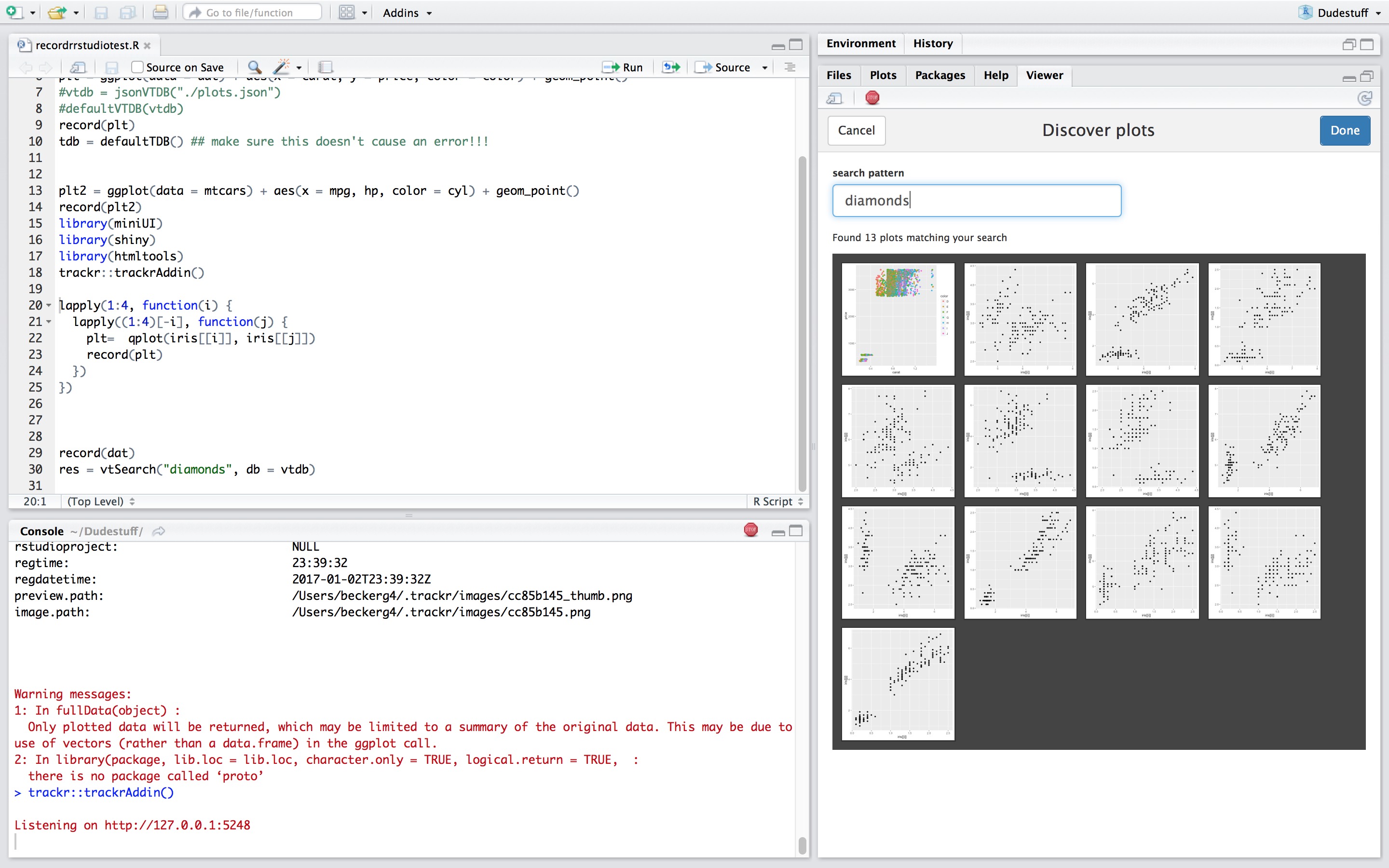
Figure 1: With the RStudio Addin version of our Shiny-based frontend, analysts can search for and view results seamlessly without leaving the RStudio IDE.

The result gallery may be a useful visualization in its own right. When viewed as a single meta-visualization, the body of results generated while analyzing a particular dataset can enable inference about higher-order relationships that are not immediately obvious from any individual result.

3.6.2 Collaborative Frontend

Blacklight (Project Blacklight 2015) is an image-gallery frontend for Solr designed to provide a visual catalog of assets for libraries and museums. Many of the features it offers out of the box align well with our goals of metadata-based search, discovery, and visual exploration. These include automatic GUI controls for faceting and restriction based on particular metadata fields, flexible paginated display of result thumbnails, bookmarking and query history tracking, and Solr’s powerful search syntax and capabilities.

In Figures 2 and 3, we see an example blacklight a gallery, and the result of searching within it for plots created using the diamonds dataset.

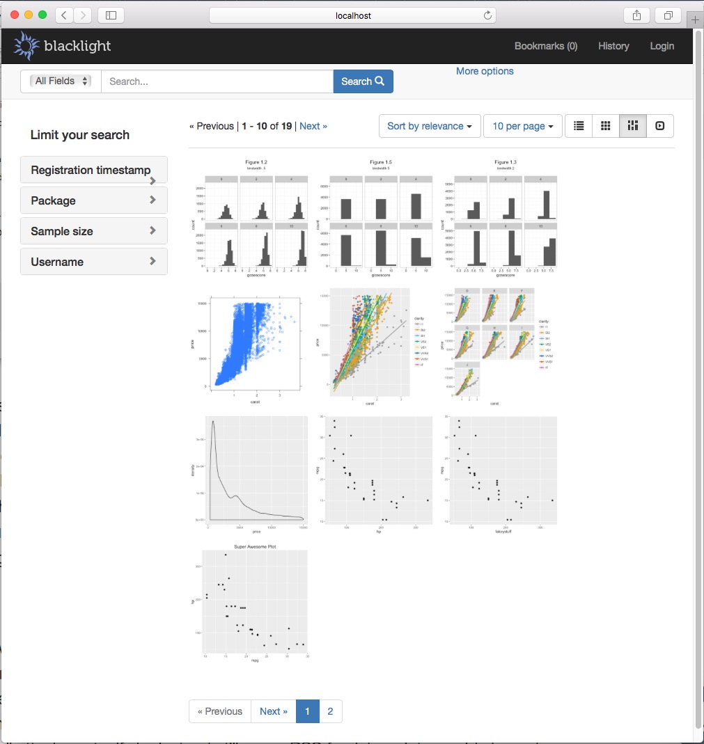
Figure 2: This blacklight gallery is running on top of a Solr core — populated by trackr — which contains visualizations of the diamonds, Chem97, and mtcars datasets.

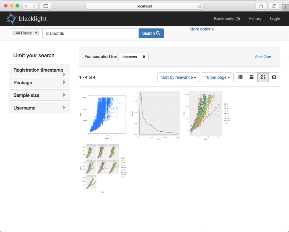
Figure 3: We use the Blacklight GUI to identify plots from our corpus which display the diamonds data. We could also do this by querying the underlying Solr core directly, or via trackr’s R API.

3.6.3 Result Feeds

When collaborating in real-time, scientists need to continually communicate their results to the rest of the group. The web technology Really Simple Syndication (RSS) is a standard mechanism for disseminating streams of content. With a standard web browser, users can view an RSS feed of updates to the result database, subject to a filter (conveniently encoded in the URL) that might restrict artifacts to plots made by a certain user, or marked with a certain tag. The RSS feed is essentially an auto-updating search, referenced by a URL. Even in the single user context, the RSS feed is useful for observing the history of an interactive analysis session. It is relatively straightforward to configure Solr to provide an RSS feed of updates.

4 Discussion

4.1 Prior Work

Examples of attaching metadata to computational artifacts are found in three related contexts: history-capture and provenance tracking within scientific visualization platforms (Brodlie et al. 1993; Heer et al. 2008; Woodruff and Stonebraker 1997), provenance capture in scientific-workflow systems (Wolstencroft et al. 2013; Callahan et al. 2006), and data sharing and archival efforts (Michener et al. 1997, 2011). Here the metadata primarly describe how the artifact was created and, in the case of datasets, what data they contain. These metadata are typically intended to enhance or ensure reproducibilty of a plot or visualization state. In the context of interaction history, this granularity can range from formally modeled high-level decisions, as in GRASPARC, to a series of individual low-level user interactions such as mouse clicks and menu selections, with many systems falling somewhere in the middle (Heer et al. 2008). In the case of general computational provenance, most specifications are relationship-based, tracking low-level details about the data, actions and entities involved in generating a dataset or result (Moreau et al. 2011; Missier et al. 2013).

Lee and Grinstein (1995) propose extending metadata capture to include the querying and manipulation of the underlying data. They further propose high-level summaries of both queries and query results, as well as their use in modeling and inferring information about an analyst’s data explorations. While their ExBase system provided this functionality only in the context of highly constrained, database-backed visualization systems, their ideas provide a core pillar of our work. Searchability of stored metadata has also come to be considered a core feature of modern provenance systems (Freire et al. 2008), generalizing the ideas of Lee and Grinstein (1995)’s vision and providing further foundation for the work we present here.

Finally, multiple services exist for sharing and publishing data visualizations and computational artifacts tagged with metadata. Figshare (Hahnel 2011) is the seminal service in this space, supporting both visualizations and general artifacts, while Plotly (Plotly Technologies Inc. 2013) is a more recent addition focused on interactive data visualizations. Despite recognizing the importance of good metadata (Figshare Support Team 2016), however, neither service annotates artifacts automatically beyond basic logistics of the submission. These services could provide alternative endpoints to our framework, allowing users to supply some or all of the metadata we generate for an artifact during submission. Similarly, metadata extracted by trackr could be used to construct submissions to provenance stores such as ProvStore (Huynh and Moreau 2014).

4.2 Limitations

4.2.1 Relying on internal representations of plot objects

Plot objects generated via the ggplot2 and lattice frameworks are intended primarily for internal consumption by those frameworks. As such, those packages do not provide official, supported APIs to extract the types of information laid out in Section 2.1.2, so we rely on implementation details that are subject to change. This incurs a substantial maintenance cost. In fact, Wickham (2009) released version 2.0.0 of the ggplot2 package during the preparation of this manuscript, rendering this limitation non-hypothetical.

4.2.2 Manual recording of artifacts

trackr requires an analyst to manually record artifacts in most cases. This can be tedious, and may overlook intermediate artifacts an analyst does not foresee needing in the future. This represents an unfortunate but ultimately necessary trade-off between effective discoverability and fully capturing the research process.

An early prototype of trackr contained an option to automatically record every plot drawn to a graphics device whenever it was loaded. We quickly found this approach to be infeasible. During data exploration, analysts often generate many similar versions of a plot or model fit before arriving at the “final” version of that artifact. These small iterations on the same artifact will typically have very similar, overlapping metadata, which can make it difficult to write simple discoverability queries that identify and return only the desired final version.

We view recording an artifact as an extension of saving it. Saving an object is typically a manual step that implies importance, and the same applies to recording. By explicitly recording an object, the analyst declares the result to noteworthy enough to warrant later retrieval.

The exception is dynamic report generation, where we automatically capture every artifact displayed in the output, based on the principle that if an artifact is important enough to be displayed in the report, it is important enough to record.

4.3 Future Directions

4.3.1 Automatic classification of plot type

Users may often want to restrict their searches to a particular class of plot — histograms, residual scatterplots used for model diagnostics, gene expression heatmaps, etc. They may be searching for a particular plot, and know it falls in that class, or may wish to discover and explore all plots of that class meeting other search criteria. For some plot types, this is relatively straightforward using the metadata we already generate. Generally speaking, however, requiring users to hand-construct search terms which indicate plot classes ranges from burdensome to infeasible, depending on the type of plot in question.

One major avenue of possible future work is automatically annotating plots with predicted plot classes and other high-level semantic inferences about their content or purpose. The low-level, plot-specific metadata we generate now could be used as inputs to a combination of hand-constructed heuristics, and statistical learning and text mining methods, in order to generate such predictions.

4.3.2 Extension to interactive graphics

Our current framework supports only static graphics, and it would be natural to extend support to interactive graphics. The specification of an interactive graphic, independent of a specific state, encodes a great deal of information in the modes of interactivity it offers. Tooltips are obviously useful as a direct visual representation of annotations, while interactive controls based on a variable or entered value encode an assumption that altering those values will change the content plotted and/or the conclusions the viewer might draw from it.

A snapshot of an interactive plot, particularly a state indicated by the user as final or particularly useful, also contains meaningful information. The parameters chosen, the subset of the data in view, the current selection, etc, are all sources of inference about the question asked and answer found by the analyst. Moreover, freezing and preserving the state of an interactive graphic, to the extent possible, would contribute to the reproducibility and discoverability of those answers.

4.3.3 Transforming static graphics into interactive ones

In addition to annotating interactive graphics, the metadata we capture about visualizations could also be used to create them. Given two plots , we could, for example, use their metadata to infer that they plot the same dataset, and then create a linked-plot combining the two. This comes as a natural extension to the holistic view of related plots use-case trackr already facilitates.

Individual static graphics can also be (re-)rendered as interactive graphics that provide GUI controls for setting particular parameters used by the code (Nolan and Temple Lang 2007; Becker 2014). A plot that displays the subset of data from a particular year, for example, might be re-rendered with a year-selector via the combination of a straightforward transformation of the code and an engine to redraw the plot. With trackr ensuring code is available, scientists could interactively explore shared results, even when the original analyst created only static data visualizations.

4.3.4 Annotating the analysis itself

It is rare that a single, independent result adequately represents the output of an entire analysis. In our experience, analyses typically produce many artifacts, each of them connected to the others through the thread of the analysis process. To capture these relationships, we need to track the analysis as a whole.

An annotated analysis might simply be a collection of annotated computational artifacts, along with the full code and data implementing the analysis. This collection would be annotated with analysis-level metadata. Some of these top-level annotations would likely be inherited directly from among the annotations of the artifacts, particularly if the system is able to identify (or is told) which artifacts are representative. Other annotations could be inferred from the number and type of artifacts the analysis generated, from combinations of annotations across artifacts, and from the full body of code that performed (and would re-perform) the analysis.

5 Conclusion

We have presented the trackr framework, consisting of our trackr and histry packages. Our framework provides three capabilities which combine to improve reproducibility, understandability, and discoverability of R-based results. First, it provides a mechanism for standardized capture and storage of results annotated with metadata. Second, it provides a mechanism for automatically extracting meaningful metadata from the results themselves as well as the code, environment, and data that generated them. Finally it provides the ability to query and search for results, based on their metadata, in multiple contexts via the presented proof-of-concept interfaces.

By automatically organizing, annotating, and indexing results, trackr enables analysts and organizations to more easily find, understand, reproduce and extend previous results, whether their own or of others, accelerating the iterative research process.

6 Availability

Up-to-date versions of our trackr and histry packages are available on Github at http://github.com/gmbecker/recordr and http://github.com/gmbecker/histry, respectively. The rdocdb dependnecy is also available on Github at http://github.com/lawremi/rdocdb; all other dependencies are available on CRAN. After responding to anything that might arise during review, they will be posted on CRAN.

References

- Allaire et al. (2016) J. Allaire, J. Cheng, Y. Xie, J. McPherson, W. Chang, J. Allen, H. Wickham, A. Atkins, and R. Hyndman. rmarkdown: Dynamic Documents for R, 2016. URL {https://CRAN.R-project.org/package=rmarkdown}. R package version 1.1.
- Becker (2014) G. Becker. Dynamic Documents for Data Analytic Science. PhD thesis, UNIVERSITY OF CALIFORNIA, DAVIS, 2014.
- Becker and Jenkins (2015) G. Becker and B. Jenkins. fastdigest: Fast, Low Memory-Footprint Digests of R Objects, 2015. URL {https://CRAN.R-project.org/package=fastdigest}. R package version 0.6-3.
- Biecek and Kosiński (2015) P. Biecek and M. Kosiński. archivist: Tools for Storing, Restoring and Searching for R Objects, 2015. URL http://CRAN.R-project.org/package=archivist. R package version 1.6.
- Brodlie et al. (1993) K. Brodlie, A. Poon, H. Wright, L. Brankin, G. Banecki, and A. Gay. GRASPARC: A Problem Solving Environment Integrating Computation and Visualization. In D. Bergeron and G. Nielson, editors, Proceedings of the 4th Conference on Visualization ’93, VIS ’93, pages 102–109, Washington, DC, USA, 1993. IEEE Computer Society. ISBN 0-8186-3940-7. URL http://dl.acm.org/citation.cfm?id=949845.949868.
- Buckheit and Donoho (1995) J. B. Buckheit and D. L. Donoho. WaveLab and Reproducible Research. In Wavelets and Statistics, pages 55–81. Springer Science Business Media, 1995. doi: 10.1007/978-1-4612-2544-7˙5. URL http://dx.doi.org/10.1007/978-1-4612-2544-7_5.
- Callahan et al. (2006) S. P. Callahan, J. Freire, E. Santos, C. E. Scheidegger, C. T. Silva, and H. T. Vo. VisTrails: Visualization Meets Data Management. In C. Yu and P. Scheuermann, editors, Proceedings of the 2006 ACM SIGMOD International Conference on Management of Data, SIGMOD ’06, pages 745–747. ACM, 2006. ISBN 1-59593-434-0. doi: 10.1145/1142473.1142574. URL http://doi.acm.org/10.1145/1142473.1142574.
- Chang et al. (2016) W. Chang, J. Cheng, J. Allaire, Y. Xie, and J. McPherson. shiny: Web Application Framework for R, 2016. URL {https://CRAN.R-project.org/package=shiny}. R package version 0.14.2.
- Claerbout and Karrenbach (1992) J. F. Claerbout and M. Karrenbach. Electronic documents give reproducible research a new meaning. In SEG Technical Program Expanded Abstracts 1992. Society of Exploration Geophysicists, jan 1992. doi: 10.1190/1.1822162. URL http://dx.doi.org/10.1190/1.1822162.
- Figshare Support Team (2016) Figshare Support Team. FAQ - How discoverable is my research?, 2016. URL https://support.figshare.com/support/solutions/articles/6000079066-how-discoverable-is-my-research-.
- Freire et al. (2008) J. Freire, D. Koop, E. Santos, and C. T. Silva. Provenance for Computational Tasks: A Survey. Computing in Science and Engg., 10(3):11–21, may 2008. ISSN 1521-9615. doi: 10.1109/MCSE.2008.79. URL http://dx.doi.org/10.1109/MCSE.2008.79.
- Gentleman and Temple Lang (2004) R. Gentleman and D. Temple Lang. Statistical Analyses and Reproducible Research. Bioconductor Project Working Papers, (2), 2004. URL http://biostats.bepress.com/bioconductor/paper2.
- Hahnel (2011) M. Hahnel. figshare - credit for all your research, 2011. URL http://figshare.com.
- Heer et al. (2008) J. Heer, J. Mackinlay, C. Stolte, and M. Agrawala. Graphical Histories for Visualization: Supporting Analysis Communication, and Evaluation. IEEE Trans. Visual. Comput. Graphics, 14(6):1189–1196, nov 2008. doi: 10.1109/tvcg.2008.137. URL http://dx.doi.org/10.1109/tvcg.2008.137.
- Huynh and Moreau (2014) T. D. Huynh and L. Moreau. Provstore: a public provenance repository. June 2014. URL http://eprints.soton.ac.uk/365509/.
- Jenkins (2012) B. Jenkins. Spookyhash: a 128-bit noncryptographic hash, 2012. URL http://burtleburtle.net/bob/hash/spooky.html.
- Lawrence et al. (2015) M. Lawrence, G. Becker, and J. Vogel. rsolr: R to Solr interface, 2015. URL {https://github.com/lawremi/rsolr}. R package version 0.0.4.
- Lee and Grinstein (1995) J. Lee and G. Grinstein. An architecture for retaining and analyzing visual explorations of databases. In Proceedings Visualization '95. Institute of Electrical & Electronics Engineers (IEEE), 1995. doi: 10.1109/visual.1995.480801. URL http://dx.doi.org/10.1109/visual.1995.480801.
- Leisch (2002) F. Leisch. Sweave: Dynamic Generation of Statistical Reports Using Literate Data Analysis. In Compstat, pages 575–580. Springer Science Business Media, 2002. doi: 10.1007/978-3-642-57489-4˙89. URL http://dx.doi.org/10.1007/978-3-642-57489-4_89.
- Michener et al. (2011) W. Michener, D. Vieglais, T. Vision, J. Kunze, P. Cruse, and G. Janée. DataONE: data observation network for earth—preserving data and enabling innovation in the biological and environmental sciences. D-Lib Magazine, 17(1/2):12, 2011.
- Michener et al. (1997) W. K. Michener, J. W. Brunt, J. J. Helly, T. B. Kirchner, and S. G. Stafford. Nongeospatial metadata for the ecological sciences. Ecological Applications, 7(1):330–342, 1997.
- Missier et al. (2013) P. Missier, K. Belhajjame, and J. Cheney. The W3C PROV family of specifications for modelling provenance metadata. In Proceedings of the 16th International Conference on Extending Database Technology - EDBT '13. Association for Computing Machinery (ACM), 2013. doi: 10.1145/2452376.2452478. URL http://dx.doi.org/10.1145/2452376.2452478.
- Moreau et al. (2011) L. Moreau, B. Clifford, J. Freire, J. Futrelle, Y. Gil, P. Groth, N. Kwasnikowska, S. Miles, P. Missier, J. Myers, B. Plale, Y. Simmhan, E. Stephan, and J. V. den Bussche. The Open Provenance Model core specification (v1.1). Future Generation Computer Systems, 27(6):743–756, jun 2011. doi: 10.1016/j.future.2010.07.005. URL http://dx.doi.org/10.1016/j.future.2010.07.005.
- Nolan and Temple Lang (2007) D. Nolan and D. Temple Lang. Dynamic, Interactive Documents for Teaching Statistical Practice. International Statistical Review, 75(3):295–321, 2007. ISSN 1751-5823. doi: 10.1111/j.1751-5823.2007.00025.x. URL http://dx.doi.org/10.1111/j.1751-5823.2007.00025.x.
- Plotly Technologies Inc. (2013) Plotly Technologies Inc. Collaborative data science, 2013. URL https://plot.ly.
- Project Blacklight (2015) Project Blacklight. Blacklight, Version 5.14.0. Charlottesville, VA, 2015. URL https://github.com/projectblacklight/blacklight.
- R Core Team (2015) R Core Team. R: A Language and Environment for Statistical Computing. R Foundation for Statistical Computing, Vienna, Austria, 2015. URL {https://www.R-project.org/}.
- Rossini and Leisch (2003) A. Rossini and F. Leisch. Literate Statistical Practice. UW Biostatistics Working Paper Series, 2003.
- (29) RStudio Inc. Shiny User Showcase. URL https://www.rstudio.com/products/shiny/shiny-user-showcase/.
- Rstudio Inc. (2012) Rstudio Inc. RPubs - Easy web publishing from R, 2012. URL https://Rpubs.com.
- Sarkar (2008) D. Sarkar. Lattice: Multivariate Data Visualization with R. Springer, New York, 2008. URL http://lmdvr.r-forge.r-project.org. ISBN 978-0-387-75968-5.
- Schwab et al. (2000) M. Schwab, M. Karrenbach, and J. Claerbout. Making scientific computations reproducible. Computing in Science & Engineering, 2(6):61–67, 2000.
- Stodden et al. (2015) V. Stodden, S. Miguez, and J. Seiler. ResearchCompendia.org: Cyberinfrastructure for Reproducibility and Collaboration in Computational Science. Computing in Science Engineering, 17(1):12–19, Jan 2015. ISSN 1521-9615. doi: 10.1109/MCSE.2015.18.
- Temple Lang et al. (2015) D. Temple Lang, R. Peng, D. Nolan, and G. Becker. CodeDepends: Analysis of R code for reproducible research and code view, 2015. URL https://github.com/duncantl/CodeDepends. R package version 0.4-2.
- Tufte and Graves-Morris (1983) E. R. Tufte and P. Graves-Morris. The visual display of quantitative information, volume 2. Graphics press Cheshire, CT, 1983.
- Wickham (2009) H. Wickham. ggplot2: elegant graphics for data analysis. Springer New York, 2009. ISBN 978-0-387-98140-6. URL http://had.co.nz/ggplot2/book.
- Wilkinson (1999) L. Wilkinson. The Grammar of Graphics. Springer-Verlag New York, Inc., New York, NY, USA, 1999. ISBN 0-387-98774-6.
- Wolstencroft et al. (2013) K. Wolstencroft, R. Haines, D. Fellows, A. Williams, D. Withers, S. Owen, S. Soiland-Reyes, I. Dunlop, A. Nenadic, P. Fisher, J. Bhagat, K. Belhajjame, F. Bacall, A. Hardisty, A. Nieva de la Hidalga, M. P. Balcazar Vargas, S. Sufi, and C. Goble. The taverna workflow suite: designing and executing workflows of web services on the desktop, web or in the cloud. Nucleic Acids Research, 41(W1):W557, 2013. doi: 10.1093/nar/gkt328. URL +http://dx.doi.org/10.1093/nar/gkt328.
- Woodruff and Stonebraker (1997) A. Woodruff and M. Stonebraker. Supporting fine-grained data lineage in a database visualization environment. In Proceedings 13th International Conference on Data Engineering, pages 91–102, Apr 1997. doi: 10.1109/ICDE.1997.581742.
- Xie (2015) Y. Xie. Dynamic Documents with R and knitr. Chapman and Hall/CRC, Boca Raton, Florida, 2nd edition, 2015. URL http://yihui.name/knitr/. ISBN 978-1498716963.