Accelerating Bayesian Structure Learning in Sparse Gaussian Graphical Models

Abstract

Gaussian graphical models are relevant tools to learn conditional independence structure between variables. In this class of models, Bayesian structure learning is often done by search algorithms over the graph space. The conjugate prior for the precision matrix satisfying graphical constraints is the well-known $G$-Wishart. With this prior, the transition probabilities in the search algorithms necessitate evaluating the ratios of the prior normalizing constants of $G$-Wishart. In moderate to high-dimensions, this ratio is often approximated using sampling-based methods as computationally expensive updates in the search algorithm. Calculating this ratio so far has been a major computational bottleneck. We overcome this issue by representing a search algorithm in which the ratio of normalizing constant is carried out by an explicit closed-form approximation. Using this approximation within our search algorithm yields significant improvement in the scalability of structure learning without sacrificing structure learning accuracy. We study the conditions under which the approximation is valid. We also evaluate the efficacy of our method with simulation studies. We show that the new search algorithm with our approximation outperforms state-of-the-art methods in both computational efficiency and accuracy. The implementation of our work is available in the R package BDgraph.

Keywords: Model Selection; $G$-Wishart; Normalizing Constants; Bayes Factors.

1 Introduction

Gaussian graphical models (GGM) have been widely used in many application areas for learning conditional independence structure among a (possibly large) collection of variables. Bayesian structure learning, for these models, while providing a natural and principled way for uncertainty quantification, often lag behind frequentist approaches (Friedman et al., 2008) in terms of computational efficiency and scalability. Despite significant developments of Bayesian structure learning methods in recent years, the scalability of these methods has continued to pose challenges regarding the growing demand for higher dimensions.

An essential element of Bayesian structure learning in GGMs is the prior distribution on the precision matrix $K$ given the graph $G$ constraints. Most Bayesian methods use the so-called $G$-Wishart distribution, which is the conjugate prior (Roverato, 2002). For structure learning, more recent Bayesian methods, use versions of search algorithms over the graph space with the capability of jointly estimate graph structure and precision matrix, see Hinne et al. (2014); Cheng and Lenkoski (2012); Lenkoski (2013); Dobra and Lenkoski (2011); Dobra et al. (2011); Wang and Li (2012); Mohammadi and Wit (2015). A computationally challenging step in these search algorithms is to estimate the ratio of prior normalizing constants for the $G$-Wishart distribution. This ratio, in general, is not available in closed form, except for specific cases, and typically needs to be evaluated using Monte Carlo based approaches. Until recently, Uhler et al. (2018) give the exact analytic expression of the normalizing constants of $G$-Wishart, which gave hope of direct evaluation of this ratio. The capability of applying this expression in the search algorithms need yet to investigate, since the expression is mathematically rather complex.

To approximate the ratio of normalizing constant, Wang (2012) introduces the double Metropolis-Hastings algorithm (Liang, 2010), by using on the block Gibbs sampler from $G$-Wishart. By using direct sampling form $G$-Wishart distribution (Lenkoski, 2013), recently, Hinne et al. (2014); Lenkoski (2013) propose more efficient versions of the search algorithms that combine the concept behind the exchange algorithm (Murray et al., 2006) with trans-dimensional MCMC algorithm (Green, 2003). Likewise, Mohammadi and Wit (2015) proposed a search algorithm over the graph space based on continuous-time birth-death processes, and following Lenkoski (2013) combined it with the exchange algorithm. These algorithms avoid to compute the ratio of normalizing constants by using the exchange algorithm; Essentially, the ratio of normalizing constants is canceling out in the probabilities of jumping to the proposal graphs, by using exact samples from the $G$-Wishart distribution. While these algorithms have clear computational benefits compared to earlier approaches, they require exact samples from the $G$-Wishart distribution, which are computationally expensive updates within the search algorithm. We are going to illustrate it in more detail in Section 2.2.

We aim to introduce a search algorithm in which the ratio of normalizing constant is evaluated by an explicit closed-form approximation. For Bayesian structure learning, we first represent the birth-death Markov Chain Monte Carlo (BDMCMC) search algorithm proposed by Mohammadi and Wit (2015). Then we provide an explicit closed-form approximation to the ratio of the prior normalizing constant of $G$-Wishart, the use of which leads to significant improvement in the scalability of the search algorithms. To immediately illustrate the accuracy, in terms of structure learning, and the computational efficiency of our proposed approximation within the search algorithm, we represent here Figure 1 where $G$ has a random graph structure with $150$ nodes ($p=150$) and a sample size of $150$. The left-hand side represents the receiver operating characteristic (ROC) plot for comparing the structure learning accuracy of the BDMCMC search algorithm done with our approximation and with the exchange algorithm. We see that our method (BDMCMC-Gamm, in blue) performs at least as well as the state-of-the-art (BDMCMC-DMH, in red). The right-hand side represents the execution time of both search algorithms. We see that for $p=150$, the execution time when using BDMCMC with our approximation is three times faster than when BDMCMC is done with the exchange algorithm. More details are given in Section 6.

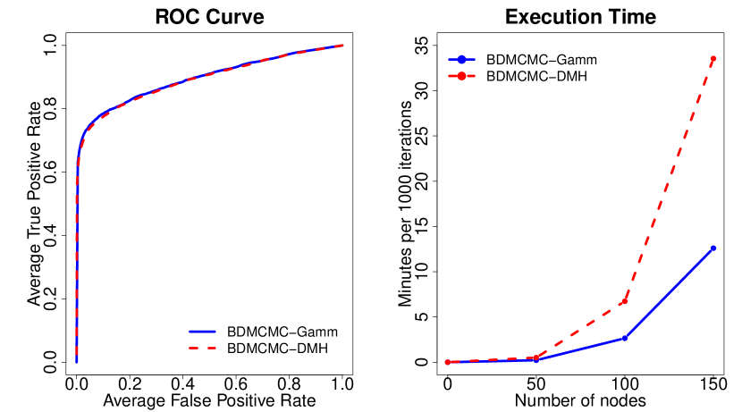
Figure 1: Plots from the simulation study in Section 6 over $50$ replications where $G$ is a random graph with $150$ nodes and sample size $150$. (Left) ROC curve for the BDMCMC search algorithm with our approximation (BDMCMC-Gamm) and the BDMCMC search algorithm with exchange algorithm (BDMCMC-DMH), as state-of-the-art. (Right) execution time for both algorithms where time is per minutes for $1000$ iterations for different number of nodes ($p=50,100,150$).

The outline of our paper is as follows. In Section 2, we introduce background materials for Bayesian structure learning in GGMs. After presenting the birth-death MCMC search algorithm in Subsection 2.1, we review the existing methods for approximating the ratio of normalizing constants in Subsection 2.2, and then we introduce our approximation. In Section 3, we provide the technical detail for proving the accuracy of the proposed approximation of the ratio of the normalizing constant. In Sections 4 and 5, we represent our two main results, Theorems 1 and 2.

In Theorem 1, we establish the approximation with explicit bounds in the particular case when all paths between the two nodes corresponding to the removed edge are disjoint (Figure 3 left-side). In Subsection 4.1, we verify the accuracy of the approximation by various collections of disjoint paths. We compute the theoretical boundary of our approximation as well as the value of the relative error following the Monte Carlo approach of Atay-Kayis and Massam (2005). We find that, while the theoretical boundary can be as high as $0.30$, the actual value of the relative error hardly goes above $0.10$ (see Figure 4).

In Theorem 2, we consider the general case where paths between the two nodes corresponding to the removed edge are not necessarily disjoint (Figure 3 right-side). In that case, we prove that under a technical assumption, our approximation is accurate. The question is then to know whether this assumption is realistic. In Subsection 5.1, for different types of graphs, we verify numerically how well this assumption holds. We also evaluate the accuracy of our approximation by simulation. To do so, we compute the ratio of the normalizing constant in two ways: first following the Monte Carlo approximation of Atay-Kayis and Massam (2005) and, second, using our approximation. We see that in all cases, both approximations take the same range of values. They are both reasonably accurate. When the number of nodes is greater than $30$, due to the limitations of the Monte Carlo approximation in Atay-Kayis and Massam (2005), one cannot numerically verify the accuracy of the approximation directly. So, in Section 6, we verify it indirectly: we use both our approximation and the exchange algorithm to compute the ratio in the BDMCMC search algorithm of Mohammadi and Wit (2015) for graphs containing $50$, $100$, or $150$ nodes. We see that in all cases, our approximation yields results as good or slightly better than the exchange algorithm as a state-of-the-art.

2 Bayesian structure learning in GGMs

Graphical models (Lauritzen, 1996) are powerful tools to express the conditional dependence structure among random variables by a graph in which each node corresponds to a random variable. For the case of undirected graphs, also known as Markov random field (Rue and Held, 2005), an edge between two nodes determines the conditional dependence of the regarding variables. Let $G=(V,E)$ be an undirected graph where $V$ contains $p$ nodes corresponding to the $p$ coordinates and the edges $E$ describe the conditional independence relationships among variables; We use the convention that if $(i,j)\in E$ then $i<j$. Let $\overline{E}$ be the complement of $E$ that indexes the missing edges of $G$.

A Gaussian graphical model for the Gaussian random vector $\mathbf{X}=(X_{1},...,X_{p})\sim\mathcal{N}_{p}(\mu,K^{-1})$ is represented by an undirected graph $G=(V,E)$. Variables $X_{i}$ and $X_{j}$ are independent given all the other variables if and only if there is no edge $(i,j)$ in $E$. It is well-known (Lauritzen, 1996) that in that case, the precision matrix $K=\Sigma^{-1}$ belongs to the cone $P_{G}$ of positive definite matrices with $K_{ij}=0$ whenever $(i,j)\in\overline{E}$. In other words, the zero entries in the off-diagonal of the precision matrix correspond to conditional independencies in the graph; It is an essential property of the precision matrix for model selection (Dempster, 1972). One can then define the GGM for a given graph $G$ as the family of distributions

$${\cal N}_{G}=\{N(0,\Sigma):K=\Sigma^{-1}\in P_{G}\}.$$

The likelihood based on a random sample $\mathbf{X}=(\mathbf{X}^{(1)},...,\mathbf{X}^{(n)})^{\top}$ from ${\cal N}_{G}$ is

$$P(\mathbf{X}|K,G)\propto|K|^{n/2}\exp\left\{\frac{-1}{2}\mbox{tr}(KS)\right\},$$

where $S=\mathbf{X}^{\top}\mathbf{X}$.

In GGMs, for Bayesian structure learning, the standard conjugate prior for the precision matrix $K$ of the Gaussian distribution is the $G$-Wishart distribution (Roverato, 2002; Letac et al., 2007). The G-Wishart is the Wishart distribution restricted to the space of precision matrices with zero entries specified by a graph $G$. The G-Wishart density $W_{G}(b,\Omega)$ is

$$P(K\mid G)=\frac{1}{I_{G}(\delta,\Omega)}|K|^{\frac{\delta-2}{2}}\exp\{\frac{-1}{2}\mbox{tr}(K\Omega)\}{\bf 1}_{P_{G}}(K),$$

where $|K|$ denotes the determinant of $K$ and the symmetric positive definite matrix $\Omega$ and the scalar $\delta>2$ are called, respectively, the scale and shape parameters. The normalizing constant

$$I_{G}(\delta,\Omega)=\int_{K\in P_{G}}|K|^{\frac{\delta-2}{2}}\exp\{\frac{-1}{2}\mbox{tr}(K\Omega)\}dK$$ (1)

is of central interest to us. For arbitrary graphs, the explicit formula for this normalizing constant is given in Proposition 1; We return to the computations of this fact in Section 3.

The joint posterior distribution of the graph $G$ and the precision matrix $K$ is given as

$$P(K,G\mid\mathbf{X}) \propto P(\mathbf{X}\mid K,G)~{}P(K\mid G)~{}P(G)$$ (2)

$$\propto P(G)~{}\frac{1}{I_{G}(\delta,\Omega)}|K|^{\frac{\delta+n-2}{2}}\exp\{\frac{-1}{2}\mbox{tr}(K(\Omega+S))\},$$

where $P(G)$ is the prior distribution of the graph $G$, which here we consider a uniform distribution over all graphs with fixed $p$ nodes, as a non-informative prior; For other options, see Dobra et al. (2011); Hinoveanu et al. (2018); Mohammadi and Wit (2015).

2.1 Structure learning via birth-death MCMC algorithm

Bayesian structure learning in GGMs which revolves around the joint posterior distribution of the precision matrix and graph (2) requires carefully designed MCMC search algorithms over the graph space. A common way to explore the graph space is by using a search algorithm known as reversible jump MCMC (RJMCMC) (Green, 1995) which is based on a discrete-time Markov chain. These kinds of algorithms often suffer from low acceptance rates since the graph space is enormous and proposals with low probabilities are frequent. Mohammadi and Wit (2015) addressed this issue by developing a continuous-time Markov chain process—or a BDMCMC search algorithm—as an alternative to RJMCMC. The BDMCMC search algorithm explores the graph space by either jumping to a larger dimension (birth) or lower dimension (death). The birth/death events are modeled as independent Poisson processes, thus the time between two successes events is exponentially distributed. The stationary distribution of the process is determined by the rates of the birth and death events that occur in continuous time; See Figure 2 for a graphical representation of birth and death events from a given graph.

In the birth and death process, given the current state $(G,K)$, each edge is added/deleted independently of the rest as a Poisson process with birth/death rate $R_{e}(G,K)$ for each $e\in\{E\cup\overline{E}\}$. Since birth and death events are independent Poisson processes, the time between two consecutive events has an exponential distribution with mean

$$W(G,K)=\frac{1}{\sum R_{e}(G,K)}$$ (3)

which is the waiting time. The waiting times capture all the possible moves of each step of the BDMCMC search algorithm. Essentially, the birth-death process tends to stay shorter in the current state for a small waiting time, while the process tends to stay longer for a large waiting time. The birth and death probabilities involved are

$$P(\mbox{birth/death of edge }e\in\{E\cup\overline{E}\})\propto R_{e}(G,K).$$ (4)

The BDMCMC seaerch algorithm converges to the joint posterior distribution (2) given the birth and death rates as a ratio of the joint posterior distributions as follows

$$R_{e}(G,K)=\min\left\{\frac{P(G^{*},K^{*}|\mathbf{x})}{P(G,K|\mathbf{x})},1\right\},\text{ for each }e\in\{E\cup\overline{E}\}.$$ (5)

For the birth of edge $e\in\overline{E}$ we take $G^{*}=(V,E\cup{e})$ and for the death of edge $e\in E$ we take $G^{*}=(V,E\setminus{e})$ and with the regarding preposition matrix is $K^{*}$. Algorithm 1 represents the pseudo-code for the BDMCMC search algorithm.

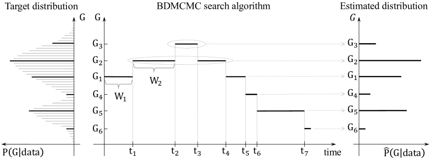
Figure 2: The left panel represents the target posterior distribution of the graphs. The middle panel shows the sampling scheme of BDMCMC algorithms in which $\left\{W_{1},W_{2},...\right\}$ stand for waiting times and $\left\{t_{1},t_{2},...\right\}$ stand for jumping times of the BDMCMC algorithm. The right panel shows the estimated posterior distribution of the graphs based on the BDMCMC sampler which are the proportional to the total waiting times of the visited graphs.

Input: A graph $G=(V,E)$ with a precision matrix $K$ and data $X$.

for $N$ iteration do

       for all the possible moves in parallel do

             Calculate the birth and death rates by Equation 5;

            

      Calculate the waiting time by Equation 3;

       Update the graph based on the birth/death probabilities in Equation 4;

       Update the precision matrix;

      

Output: Samples from the joint posterior distribution (2).

Algorithm 1 BDMCMC search algorithm

The essential element of the BDMCMC search algorithm is that a continuous-time jump process is associated with the birth and death rates. Whenever a jump occurs, the corresponding move is always accepted, which can consider as more intelligent navigation of the graph space. The acceptance probabilities of commonly used RJMCMC algorithms are replaced by the waiting times in the BDMCMC algorithm. Correspondingly, graphs with high posterior probabilities have larger waiting times while graphs with low posterior probabilities have small waiting times and as a result, die quickly. Another computational advantage of the BDMCMC algorithm is that the nested for loop, as a computationally expensive part of the algorithm, for computing the birth/death rates can be implemented in parallel since the rates associated with each edge can be calculated independently of each other. We have implemented this part in parallel in the current version of the R package BDgraph (Mohammadi and Wit, 2019a). These properties make the BDMCMC algorithm an efficient search approach to explore the graph space to identify the high posterior probability regimes, particularly for high-dimensional graphical models.

The main computational bottleneck of Algorithm 1 is to evaluate the birth/death rates, which are based on the ratio of the posterior probabilities. These birth/death rates can be considered as the conditional Bayes factor of the comparison between graph $G$ and $G^{+e}$/$G^{-e}$, similar to Hinne et al. (2014). These ratios in Equation 5 can be derived as

$$\frac{P(G^{*},K^{*}|\mathbf{x})}{P(G,K|\mathbf{x})}=\frac{I_{G}(\delta,\Omega)}{I_{G^{*}}(\delta,\Omega)}H(K,\Omega+S,\delta+n,e),$$

where

$$H(K,\Omega+S,\delta+n,e)=\left(\frac{|K^{*}|}{|K|}\right)^{\frac{\delta+n}{2}-1}\frac{\exp\{\frac{-1}{2}\mbox{tr}(K^{*}(\Omega+S))\}}{\exp\{\frac{-1}{2}\mbox{tr}(K(\Omega+S))\}}.$$ (6)

For details regarding how to compute the above function, see Cheng and Lenkoski (2012); Mohammadi and Wit (2015); Hinne et al. (2014). We see that computing the ratio of posteriors requires evaluating the ratio of prior normalizing constants. That is the main computational bottleneck of these types of search algorithms.

2.2 Existing methods to compute the normalizing constant

Exact formula: Recently, Uhler et al. (2018) certify that it is possible to drive an explicit expression for the intractable normalizing constant for general graphs. Since the expression is (by its nature) mathematically complex, the capability of applying this intricate expression for Bayesian structure learning has yet to be investigated. One possibility, as they point it out, would be to find more computationally efficient procedures than Uhler et al. (2018, Theorem 3.3) for computing the normalizing constant for particular classes of graphs.

Monte Carlo approximation: Atay-Kayis and Massam (2005) developed a Monte Carlo (MC) approach to approximate the normalizing constant based on the decomposition described in Section 3. Although the MC approximation is accurate, it can be computationally expensive. In our simulation of Sections 4.1 and 5.1, we faced numerical and computational issues of MC approximation for $p$ higher than 30.

Laplace approximation: Lenkoski and Dobra (2011) developed a Laplace approximation to compute $I_{G}(\delta,\Omega)$. Their approximation is based on using the iterative proportional scaling algorithm for computing the mode of the integral in Equation 1. This approximation is computationally faster than the MC approach, though it tends to be accurate only for the case of computing the posterior normalizing constant.Thus, they suggest using the Laplace approximation (as a computationally fast but less accurate approach) for the posterior normalizing constant and the MC integration (as a computationally expensive but more accurate approach) for the prior normalizing constant.

Exchange algorithm: Murray et al. (2006) proposed the exchange algorithm for simulating from distributions, where prior distributions–like $G$-Wishart– have intractable normalizing constants that varies according to the model. These types of algorithms are also known as auxiliary variable approaches since they require exact sampling from the auxiliary variable to canceling out the ratio of normalizing constant in the Metropolis-Hastings acceptance probabilities (Park and Haran, 2018). Hinne et al. (2014); Lenkoski (2013); Mohammadi and Wit (2015) have implemented this algorithm in GGMs to avoid normalizing constant calculation by using the exact sampler algorithm from $G$-Wishart distribution, proposed by Lenkoski (2013). As state-of-the-art, this development has proven to yield significant computational improvement as it avoids the need for expensive approximations within the search algorithm. We briefly review the implementation of the exchange algorithm within the search algorithm; For more details, see (Wang, 2012, Section 5.2).

Suppose we want to compute the birth/death rate (5) for graph $G=(V,E)$ with the precision matrix $K$ as a current state of the search algorithm. By using the exchange algorithm, we can replace the intractable normalizing constant ratio with an estimate from a single sample at each parameter setting as

$$\frac{I_{G}(\delta,\Omega)}{I_{G^{*}}(\delta,\Omega)}\approx\frac{|\widetilde{K}|^{\frac{\delta}{2}-1}\exp\{\frac{-1}{2}\mbox{tr}(\widetilde{K}\Omega)\}}{|\widetilde{K}^{*}|^{\frac{\delta}{2}-1}\exp\{\frac{-1}{2}\mbox{tr}(\widetilde{K}^{*}\Omega)\}}$$

where $\widetilde{K}$ has to be an exact sampler from the prior distribution, $W_{G}(\delta,\Omega)$. The exchange algorithm replaces the ratio of the intractable normalizing constants with an estimate from a single sample at each parameter setting. By using the above approximation, the birth/death rates will be

$$R_{e}(G,K)\approx\min\left\{\frac{H(K,\Omega+S,\delta+n,e)}{H(\widetilde{K},\Omega,\delta,e)},1\right\},\text{ for each }e\in\{E\cup\overline{E}\},$$ (7)

where function $H$ is given in Equation 6. Essentially, the intractable prior normalizing constants have been replaced by an evaluation of function $H$ at $\widetilde{K}$ as an exact sample from the prior distribution $W_{G}(\delta,\Omega)$.

Algorithm 2 represents the pseudo-code for the BDMCMC search algorithm combined with the exchange algorithm to compute the ratio of normalizing constant. We call it a double BDMCMC algorithm and consider it here as state-of-the-art. For more details, see Mohammadi and Wit (2015); Hinne et al. (2014).

Input: A graph $G=(V,E)$ with a precision matrix $K$ and data $X$.

for $N$ iteration do

       Draw $\widetilde{K}\thicksim W_{G}(\delta,\Omega)$;

       for all the possible moves in parallel do

             Calculate the birth and death rates by Equation 7 ;

            

      Calculate the waiting time by Equation 3 ;

       Update the graph based on birth/death probabilities in Equation 4 ;

       Update the precision matrix;

      

Output: Samples from the posterior distribution (2).

Algorithm 2 Double BDMCMC algorithm

Remark 1.

Algorithm 2 requires exact sampling from the prior distribution of $G$-Wishart as a computationally expensive update within the BDMCMC search algorithm. Exact sampling from $G$-Wishart distribution, following Lenkoski (2013), can be done by first sampling a standard Wishart variable from a full model and then using the iterative proportional scaling algorithm to place the variable in the correct space. It requires the solution of systems involving large matrices, in particular the inverse calculation of matrix $K$.

2.3 Proposed method to compute the normalizing constant

To bypass the computational bottleneck from the intractable normalizing constant in Algorithm 1, we represent a simple explicit analytic formula to approximate the normalizing constant as

$$\frac{I_{G^{-e}}(\delta,\mathbb{I}_{p})}{I_{G}(\delta,\mathbb{I}_{p})}\approx\frac{1}{2\sqrt{\pi}}\frac{\Gamma(\frac{\delta+d}{2})}{\Gamma(\frac{\delta+d+1}{2})}$$ (8)

where $d$ is the number of paths of length two linking the endpoints of $e$. As is the case most of the time, in the absence of prior information, the parameter $\Omega$ is taken to be the $p$-dimensional identity matrix $\mathbb{I}_{p}$; Throughout, we set $\Omega=\mathbb{I}_{p}$. This approximation is exact in some cases, as we mentioned in Remark 4. The following sections are therefore devoted to proving this approximation and analyzing its accuracy.

3 The ratio of normalizing constants

We first recall a result by Atay-Kayis and Massam (2005) which expresses $I_{G}(\delta,\Omega)$ as the product of a constant and an expectation. Let $K$ be the precision matrix and $K=\Psi^{t}\Psi$ its Cholesky decomposition where $\Psi$ is upper triangular with positive diagonal elements. Given the fact $K_{ij}=0$ for $(i,j)\in\overline{E}$, through simple matrix multiplication, we can verify

$$\psi_{E}=\{\psi_{ij}:(i,j)\in E\;\&\;\psi_{ii}:i\in V\}$$

is in 1-1 correspondence with $K_{E}=\{K_{ij}:(i,j)\in E\;\&\;K_{ii}:i\in V\}$. Also, the entries of $\psi_{\overline{E}}=\{\psi_{ij}:(i,j)\in\overline{E}\}$ can be expressed in terms of $\psi_{E}$, a fact used in Proposition 1 below. Thus the entries of $\psi_{E}$ are called free variables while the entries of $\psi_{\overline{E}}$ are non-free variables. Using the change of variables from $K_{E}$ to $\psi_{E}$, Atay-Kayis and Massam (2005) prove the normalizing constant $I_{G}(\delta,\Omega)$ can be expressed as a known constant multiplied by the expected value of a function of $\psi_{E}$. In the particular case where $\Omega=\mathbb{I}_{p}$, which is of concern to us, the result is as follows.

Proposition 1.

For each node $i=\{1,\ldots,p\}$ of the undirected graph $G$, let $\nu_{i}$ be the number of neighbours of $i$ which have a numbering larger than or equal to $i+1$. Then we have

$$I_{G}(\delta,\mathbb{I}_{p})=\left[\prod_{i=1}^{p}\pi^{\frac{\nu_{i}}{2}}2^{\frac{\delta}{2}+\nu_{i}}\Gamma\left(\frac{\delta+\nu_{i}}{2}\right)\right]\mathbb{E}\left(e^{-\frac{D}{2}}\right)$$

where

$$D=\sum_{(i,j)\in\overline{E}}\psi_{ij}^{2}.$$

The expected value is taken with respect to a product of independent random variables $\psi_{ij}\sim N(0,1)$ where $(i,j)\in E$ and random variables $\psi_{ii}^{2}\sim\chi^{2}_{\delta+\nu_{i}}$ where $i=\{1,\ldots,p\}$.

The value of $I_{G}(\delta,\mathbb{I}_{p})$ is independent of the ordering of the nodes, so without loss of generality, in the remainder of this paper, we assume the nodes defining the edge $e$ are $q=p-1$ and $p$, that is the endpoints of $e$ are numbered last. For convenience, we write $\psi_{e}=\psi_{qp}$, which is a non-free variable in the graph $G^{-e}$.

Corollary 1.

Let $G^{-e}$ be the graph obtained from $G$ by removing the edge $e=(q,p)$. The ratio of the prior normalizing constants for $G^{-e}$ and $G$ is

$$\frac{I_{G^{-e}}(\delta,\mathbb{I}_{p})}{I_{G}(\delta,\mathbb{I}_{p})}=\frac{1}{2\sqrt{\pi}}\frac{\Gamma(\frac{\delta}{2})}{\Gamma(\frac{\delta+1}{2})}\frac{\mathbb{E}\left(e^{\frac{-1}{2}\left(D+\psi_{e}^{2}\right)}\right)}{\mathbb{E}\left(e^{\frac{-1}{2}D}\right)}.$$ (9)

Let $nb(i)$ denote the set of neighbours of $i\in V$ for $i=\{1,\ldots,p\}$. The proof of Corollary 1 is immediate if we observe that, since $\nu_{i}=|nb(i)\cap\{i+1,\ldots,p\}|$, the only $\nu_{i}$ that changes between $G^{-e}$ and $G$ is the node $\nu_{q}$ and, clearly, $\nu_{q}^{G^{-e}}=0$ while $\nu_{q}^{G}=1$.

3.1 Reformulation of the ratio of normalizing constants

We can drive the non-free entries of $\psi$ as

$$\psi_{1j}=0\;\;\;\text{and}\;\;\;\psi_{ij}=\frac{-1}{\psi_{ii}}\sum_{l=1}^{i-1}\psi_{li}\psi_{lj},\;i\not=1.$$ (10)

The variables $\psi_{li}$ or $\psi_{lj}$ in the expression of $\psi_{ij}$ above may be free or non-free variables; see also Atay-Kayis and Massam (2005, Proposition 2).

Remark 2.

If $\psi_{ij}$ is non-free, it follows from Equation 10 that $\psi_{ij}$ can only be function of free variables $\psi_{lk},l\not=k$ such that $l\leq i$ and $k<j$ and $\psi_{ll},l\leq i$.

Since the value of $I_{G}(\delta,\mathbb{I}_{p})$ does not depend upon the order of the nodes, from now on in this paper, we assume the nodes which are neighbours to both $q$ and $p$, are numbered $p-1-d,p-1-(d-1),\ldots,p-1-1$ where $d$ is the number of paths of length 2 between nodes $q$ and $p$; See for example the node orders in Figure 3. With this convention, we have $\psi_{e}=A+b$ where

$$A =\frac{-1}{\psi_{qq}}A_{1}\;\;\text{ where }\;\;A_{1}=\sum^{q-1}_{l=q-d}\psi_{lq}\psi_{lp},$$ (11)

$$b =\frac{-1}{\psi_{qq}}b_{1}\;\;\;\text{ where }\;\;\ b_{1}=\sum^{q-(d+1)}_{l=1}\psi_{lq}\psi_{lp}.$$ (12)

Remark 3.

The numbering we have adopted for nodes that are neighbours both to $q$ and $p$ ensures that $A$ is independent of $b$ and $D$.

With the notations above, Equation 9 can be written

$$\frac{I_{G^{-e}}(\delta,\mathbb{I}_{p})}{I_{G}(\delta,\mathbb{I}_{p})}=\frac{1}{2\sqrt{\pi}}\frac{\Gamma(\frac{\delta}{2})}{\Gamma(\frac{\delta+1}{2})}\frac{\mathbb{E}\left(e^{-\frac{D}{2}}e^{-\frac{(A+b)^{2}}{2}}\right)}{\mathbb{E}\left(e^{-\frac{D}{2}}\right)}.$$

Our aim is to approximate this ratio and, towards this goal, we have the following approximation

$$\mathbb{E}\left(e^{-\frac{D}{2}}e^{-\frac{(A+b)^{2}}{2}}\right)\approx\mathbb{E}\left(e^{-\frac{D}{2}}\right)\mathbb{E}\left(e^{-\frac{A^{2}}{2}}\right).$$ (13)

If we prove that the above approximation holds, then we will have

$$\frac{I_{G^{-e}}(\delta,\mathbb{I}_{p})}{I_{G}(\delta,\mathbb{I}_{p})}\approx\frac{1}{2\sqrt{\pi}}\frac{\Gamma(\frac{\delta}{2})}{\Gamma(\frac{\delta+1}{2})}\mathbb{E}\left(e^{-\frac{A^{2}}{2}}\right).$$

Regarding Proposition 2 of the Supplementary File, we have the analytic expression

$$\mathbb{E}\left(e^{-\frac{A^{2}}{2}}\right)=\frac{\Gamma(\frac{\delta+1}{2})}{\Gamma(\frac{\delta}{2})}\frac{\Gamma(\frac{\delta+d}{2})}{\Gamma(\frac{\delta+d+1}{2})}$$

and thus we have

$$\frac{I_{G^{-e}}(\delta,\mathbb{I}_{p})}{I_{G}(\delta,\mathbb{I}_{p})}\approx\frac{1}{2\sqrt{\pi}}\frac{\Gamma(\frac{\delta+d}{2})}{\Gamma(\frac{\delta+d+1}{2})}$$

which is the approximation (8) that we want to prove.

Remark 4.

It is important to note that in Equation 13 if $b=0$, then our approximation (8) is exact. This means that when there are only paths of length 2, or no path, between nodes $q$ and $p$, the approximation is exact. It is interesting to note that this happens also in other cases. In fact, Uhler et al. (2018, Theorem 2.5) show that if $G^{-e}$ is such that $G$ is decomposable, then our approximation (8) is exact.

Lemma 1.

Using the quantities, $D$, $A$, $b$, and $b_{1}$ defined above, we have

$$\mathbb{E}\left(e^{-\frac{D}{2}-\frac{(A+b)^{2}}{2}}\right)=\mathbb{E}\left(e^{-\frac{A^{2}}{2}}\right)\mathbb{E}\left(e^{-\frac{D}{2}}\mathbb{E}\left(h\left(b_{1},\delta^{*}\right)\big{|}\Psi_{\cup}^{-}\right)\right),$$

where $\delta^{*}=\frac{\delta+d}{2}$ and

$$h(b_{1},\delta^{*})=\frac{2^{-\delta^{*}}}{\Gamma(\delta^{*})}\int_{0}^{+\infty}y^{\delta^{*}-1}e^{\frac{-1}{2}\left(y+\frac{b_{1}^{2}}{y}\right)}dy,$$ (14)

and

$$\Psi_{\cup}^{-}=\{\psi_{ij}:(i,j)\in E\setminus\left(E_{q}\cup E_{p}\right)\}.$$ (15)

where $E_{q}=\{(i,j):(i,q)\in E\}$ and $E_{p}=\{(i,j):(i,p)\in E\}$. $\Psi_{\cup}^{-}$ includes all the free elements of the matrix $\Psi$ except those are the neighbors of nodes $p$ and $q$.

The proof is given in Section B of the Supplementary file. Regarding to the above lemma, proving

$$\mathbb{E}\left(e^{-\frac{D}{2}}\mathbb{E}\left(h\left(b_{1},\delta^{*}\right)\big{|}\Psi_{\cup}^{-}\right)\right)\approx\mathbb{E}\left(e^{-\frac{D}{2}}\right)$$

leads to the approximation in Equation 13. For convenience, we will also adopt the notation

$$I_{1}=\mathbb{E}\left(e^{-\frac{D}{2}}\mathbb{E}\left(h\left(b_{1},\delta^{*}\right)\big{|}\Psi_{\cup}^{-}\right)\right)\;\ \text{and}\;\;I_{2}=\mathbb{E}\left(e^{-\frac{D}{2}}\right).$$

and therefore

$$\frac{I_{1}}{I_{2}}=\frac{\mathbb{E}\left(e^{-\frac{D}{2}}\mathbb{E}\left(h\left(b_{1},\delta^{*}\right)\big{|}\Psi_{\cup}^{-}\right)\right)}{\mathbb{E}\left(e^{-\frac{D}{2}}\right)}.$$ (16)

Note that the accuracy of our approximation in Equation 8 is represented by how close is the above ratio $I_{1}/I_{2}$ to 1. Thus, proving that our approximation is accurate is equivalent to prove that $I_{1}/I_{2}$ can accurately be approximated by 1. For example, for the cases that $I_{1}/I_{2}$ is equal to 1, our approximation is exact.

Remark 5.

It is important to mention that $I_{1}/I_{2}$ is always equal to or less than 1 ($I_{1}/I_{2}\leq 1$). It follows immediately from Equation 14 since $b_{1}^{2}/Y$ is always positive and $e^{-b_{1}^{2}/Y}\leq 1$.

Remark 6.

If we could show, whatever the value of $\Psi_{\cup}^{-}$, the expectation $\mathbb{E}\left(h\left(b_{1},\delta^{*}\right)\big{|}\Psi_{\cup}^{-}\right)$ can uniformly be approximated by $1$, it would follow that $I_{1}/I_{2}$ can also be approximated by $1$. We are not able to quite achieve this goal but, first, in the next Section (Theorem 1), we establish the approximation with explicit bounds in the special case when all paths between $q$ and $p$ are disjoint. The key to proving this result is the fact that $b_{1}$ can be expressed as a linear product of independent normal variables, for the cases of disjoint paths. Then, in Section 5, we show, conditional on $\Psi_{\cup}^{-}$ defined in Equation 15, the distribution of $b_{1}$ is a scale mixture of normal distributions. We then use this scale mixture of distributions to admit a unique $N(0,v_{D})$ approximation. Finally, we show that a sufficient condition for $\mathbb{E}\left(h(b_{1},\delta^{*})\big{|}\Psi_{\cup}^{-}\right)$ to be close to $1$ is that $v_{D}$ is close to $0$.

4 The ratio for the case disjoint paths

A path is a sequence of nodes in which each node is connected by an edge to the next and the path length is the number of edges between them. Two paths between $q$ and $p$ are disjoint if they have no node other than $p$ and $q$ in common. For example, in the left-hand side graph of Figure 3, the paths between $q=7$ and $p=8$ are

$$\lambda_{1}=\{q,1,2,3,p\},\;\;\lambda_{2}=\{q,4,5,p\},\;\;\lambda_{3}=\{q,6,p\},$$

and they are disjoint paths.

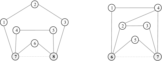
Figure 3: (Left) A graph with disjoint paths between $q$ and $p$. (Right) A graph with several non-disjoint paths between $q$ and $p$.

A path $\lambda\in\Lambda$ of length $\ell_{\lambda}+1$ is a sequence of distinct nodes as $\lambda=\{q,1_{\lambda},2_{\lambda},\ldots,\ell_{\lambda},p\}$ where $(q,1_{\lambda}),\ldots,(i_{\lambda},(i+1)_{\lambda}),\ldots,(\ell_{\lambda},p)$ are edges of $G$; The set of all such paths $\lambda$ between $q$ and $p$ is denoted $\Lambda$. We let $E_{\lambda}$ and $V_{\lambda}$ be, respectively, the set of edges, the set of interior nodes of $\lambda$ and the set of interior points deprived of $1_{\lambda}$, i.e.

$$E_{\lambda}=\left\{(q,1_{\lambda}),(1_{\lambda},2_{\lambda}),\ldots,(\ell_{\lambda},p)\right\},\;\;V_{\lambda}=\{1_{\lambda},2_{\lambda},\ldots,\ell_{\lambda}\}.$$

If $L=|\Lambda|$ is the total number of paths, we set an arbitrary order $\lambda_{1},\ldots,\lambda_{L}$ of the paths where, for convenience, we list the paths of length 2, i.e. $\ell_{\lambda}=1$ last. The nodes $q$ and $p$ are ranked last so that the order of the nodes in $V$ is

$$1_{\lambda_{1}},\ldots,\ell_{\lambda_{1}},1_{\lambda_{2}},\ldots,\ell_{\lambda_{2}},\ldots,\ldots,1_{\lambda_{L}},\ldots,\ell_{\lambda_{L}},q,p.$$

Using these notations, the following lemma gives the expression for $\psi_{e}$ in terms of the free variables $\psi_{E}$.

Lemma 2.

In the model with underlying graph $G^{-e}$, the variables $\psi_{qp}=\psi_{e}$ of the Cholesky decomposition of the precision matrix $K$ is expressed in terms of $\psi_{E}$ as

$$\psi_{e}=\frac{1}{\psi_{qq}}\sum_{\lambda\in\Lambda}(-1)^{\ell_{\lambda}}\frac{\prod_{a\in E_{\lambda}}\psi_{a}}{\prod_{v\in V_{\lambda}\setminus\{1_{\lambda}\}}\psi_{vv}}.$$ (17)

The proof relies on a repeated application of Equation 10. The proof is given in Section C of the Supplementary file. We illustrate these calculations with the following example.

Example 1.

Consider the graph of Figure 3 (left). The upper triangular matrix $\Psi$ is

$$\Psi=\begin{bmatrix}\psi_{11}&\psi_{12}&0&0&0&0&\psi_{17}&0\\ &\psi_{22}&\psi_{23}&0&0&0&*&0\\ &&\psi_{33}&0&0&0&*&\psi_{38}\\ &&&\psi_{44}&\psi_{45}&0&\psi_{47}&0\\ &&&&\psi_{55}&0&*&\psi_{58}\\ &&&&&\psi_{66}&\psi_{67}&\psi_{68}\\ &&&&&&\psi_{77}&*\\ &&&&&&&\psi_{88}\end{bmatrix}$$

where the entries marked with a “$*$” are the non-free entries and are given as

$$\psi_{27}=-\frac{\psi_{12}\psi_{17}}{\psi_{22}},\;\;\psi_{37}=\frac{\psi_{17}\psi_{12}\psi_{23}}{\psi_{22}\psi_{33}},\;\;\psi_{57}=-\frac{\psi_{45}\psi_{47}}{\psi_{55}},$$

and

$$\psi_{78} =-\frac{1}{\psi_{77}}\left(\psi_{67}\psi_{68}+\psi_{57}\psi_{58}+\psi_{37}\psi_{38}\right)$$

$$=\frac{1}{\psi_{77}}\left(-\psi_{67}\psi_{68}+\frac{\psi_{47}\psi_{45}\psi_{58}}{\psi_{55}}-\frac{\psi_{17}\psi_{12}\psi_{23}\psi_{38}}{\psi_{22}\psi_{33}}\right).$$

Equation 17 is verified. We see that the different terms in $\psi_{qp}=\psi_{78}$ above concern, successively, the paths of length 2, 3, and 4.

We are now in a position to state and prove the first of our two main results regarding the error made of our approximation in Equation 8 or equivalently the approximation in Equation 13.

Theorem 1.

For the case where in the graph $G$ the paths between the endpoints of the edge $e=(q,p)$ are disjoint, the ratio $I_{1}/I_{2}$ (16) is such that

$$B(\delta,d,\ell_{\lambda})\leq\frac{I_{1}}{I_{2}}\leq 1,$$ (18)

where

$$B(\delta,d,\ell_{\lambda})=1-\frac{\delta^{2}}{\pi(\delta+2)}\left(\frac{\Gamma(\frac{\delta}{2})}{\Gamma(\frac{\delta+1}{2})}\right)^{2}r(\delta+d-1)\sum_{\lambda\in\Lambda}{r(\delta)}^{\ell_{\lambda}},$$ (19)

with $\Lambda$ being the set of paths between $q$ and $p$, $d$ the number of paths of length 2, and

$$r(\delta)=\frac{\Gamma(\frac{\delta}{2})}{\sqrt{\pi}\Gamma(\frac{\delta+1}{2})}.$$

With an accuracy given by Equation 18, we have the approximation

$$\frac{I_{G^{-e}}(\delta,\mathbb{I}_{p})}{I_{G}(\delta,\mathbb{I}_{p})}\approx\frac{1}{2\sqrt{\pi}}\frac{\Gamma(\frac{\delta+d}{2})}{\Gamma(\frac{\delta+d+1}{2})}.$$

Proof. The proof is given in Section D of the Supplementary file. The proof is based on the fact that the expression of $b_{1}$ (12) can be expressed as a linear product of independent normal variables in the case the paths between $q$ and $p$ are disjoint.

4.1 Simulated experiments for the case of disjoint paths

To illustrate the results in Theorem 1, we report the ratio $I_{1}/I_{2}$ (16) following the MC approach of Atay-Kayis and Massam (2005) as well as the lower bound $B$ in Equation 19. We note that, if $I_{1}/I_{2}\approx 1$ our approximation is good, without any additional conditions. Note that, $1-I_{1}/I_{2}$ reflects the error rate of our approximation (8) for the prior normalizing constant of $G$-Wishart. Since $I_{1}/I_{2}$ and $B$ are functions of $\delta$ and type of disjoint paths ($d$ and $\ell_{\lambda}$), our simulation is based on graphs with different types of disjoint paths as well as different values of $\delta$. We consider $15$ different types of graphs with five different paths between $q$ and $p$. These graphs are indicated on the horizontal axis in Figure 4. Each sequence of four digits denotes the number of paths of length $2$, $3$, $4$, and $5$ in the graphs. For example, “$3110$” indicates a graph configuration with $3$ disjoints paths of length $2$, $1$ of length $3$, $1$ of length $4$, and $0$ of length $5$.

Figure 4 represents the values of $I_{1}/I_{2}$ (over $100$ replications) as well as the lower bound $B$ (19) for two values of $\delta=3$ and $\delta=10$. The worst-case scenarios are for the case $\delta=3$ and no paths of length two ($d=0$), likes the graph “$0500$” which has $5$ paths of length $3$ and no other type of paths; These types of graphs are highly unlikely cases. Even for this case, the relative error is around $0.12$. For the case $\delta=10$, we see that our approximation has pretty good performance with the maximum relative error $1-I_{1}/I_{2}$ around $0.025$.

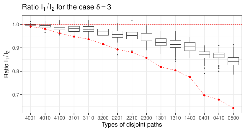
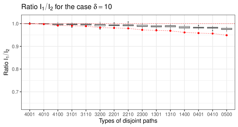
Figure 4: The ratio $I_{1}/I_{2}$ and its bound $B$ in Equation 19 for $\delta=3$ (top) and $\delta=10$ (bottom). The red dotted line is the lower bound $B$ and the boxplots are the $I_{1}/I_{2}$ computed by the MC algorithm of Atay-Kayis and Massam (2005), with over 100 replications. The $15$ different graphs are indicated on the horizontal axis. Each sequence of four digits indicates the number of paths of lengths 2, 3, 4, and 5 in the graph. For example, “$3110$” represents a graph with $3$ disjoints paths of length $2$, $1$ of length $3$, $1$ of length $4$, and $0$ of length $5$.

Figure 5 reports the values of the lower bound $B$ for different values of $\delta$ ($\delta=\{3,4,...,40\}$) and for the $15$ different graphs which are indicated on the horizontal axis in Figure 4. Each dotted line represents the $B$ values for a specific graph with different type of paths. For instance, the black bottom line is for the configuration “$0500$”. In general, this plot indicates that the accuracy of our approximation is increased by increasing the value of $\delta$. As we can see the worst-case scenario is for the minimum value of $\delta$($=3$), while for the cases $\delta>10$ the lower bound $B$ for our approximation is cloth to 1.

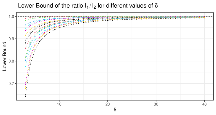
Figure 5: Plot visualization for the lower bound $B$ (19) for $\delta=\{3,4,...,40\}$ and for the $15$ different graphs which are indicated on the horizontal axis in Figure 4. Each dotted line represents the $B$ values for a graph with specific types of paths. For example, the black bottom line is for the case “$0500$” which means a graph with $0$ disjoints paths of length $2$, $5$ of length $3$, $0$ of length $4$, and $0$ of length $5$.

5 The ratio in general case

When the paths between $q$ and $p$ are not disjoint, the expression of $b_{1}$ (12) becomes more complicated. It can be expressed in terms of variables $\psi_{jp}\sim N(0,1),j<p$ and variables of the type

$$X_{ij}=\frac{\psi_{ij}}{\psi_{jj}},\;\;i<j,$$

where $\psi_{ij}\sim N(0,1)$ and $\psi_{jj}^{2}\sim\chi^{2}_{\delta+\nu_{j}}$. As a toy example, for the graph of Figure 3 (right) with tedious computations yield

$$b_{1}=\psi_{26}X_{23}^{2}X_{24}\psi_{47}+\psi_{26}X_{24}\psi_{47}+\psi_{16}X_{14}\psi_{47}+\psi_{26}X_{23}\psi_{37}.$$

For the details, see Example 2 in Section E.1 of the Supplementary File. We see that $b_{1}$ is the sum of polynomials in $X_{ij},(i,j)\in E$ multiplied by the product of two independent $N(0,1)$. But, unlike in the case of disjoint paths between $q$ and $p$, the polynomials here are not linear in each $X_{ij}$; We see in our simple example that one of them has degree 2, and larger graphs would lead to polynomials of higher linear degree. So, we could not find a lower bound, similar to Theorem 1. We therefore should find another argument to prove that $I_{1}/I_{2}$ is close to $1$. This result is given in the following Theorem as the second main result of the paper.

Theorem 2.

Under the approximation $b_{1}\sim N(0,v_{D})$, the ratio $I_{1}/I_{2}$ (16) can be written

$$\frac{I_{1}}{I_{2}}=\frac{\mathbb{E}\left(e^{-\frac{D}{2}}g\left(\delta^{*},v_{D}\right)\right)}{\mathbb{E}(e^{-\frac{D}{2}})},$$ (20)

where

$$g\left(\delta^{*},v_{D}\right)=\frac{\left(\frac{v_{D}}{2}\right)^{\delta^{*}}}{\Gamma(\delta^{*})}\int_{0}^{\infty}t^{\delta^{*}-\frac{1}{2}}(1+t)^{\frac{-1}{2}}e^{-\frac{v_{D}t}{2}}dt,$$

in which $\delta^{*}=\frac{\delta+d}{2}$. Moreover, when $v_{D}$ is small, we have

$$g\left(\delta^{*},v_{D}\right)=1-\frac{\Gamma\left(\delta^{*}+\frac{1}{2}\right)}{\Gamma\left(\delta^{*}\right)}\left(\frac{v_{D}}{2}\right)^{\delta^{*}}{\mathcal{O}}\left(\left|\frac{v_{D}}{2}\right|^{\delta^{*}-1}\right).$$

And when, for all $D$, $v_{D}$ is uniformly bounded by a small quantity, we have

$$\frac{I_{1}}{I_{2}}=1-\frac{\Gamma\left(\delta^{*}+\frac{1}{2}\right)}{\Gamma\left(\delta^{*}\right)}\frac{\mathbb{E}\left(e^{-\frac{D}{2}}\left(\frac{v_{D}}{2}\right)^{\delta^{*}}{\mathcal{O}}(|\frac{v_{D}}{2}|^{\delta^{*}-1})\right)}{\mathbb{E}(e^{-\frac{D}{2}})}\ \approx 1\;$$

and it leads that our approximation (8) holds.

Proof. The proof is in three steps. First, we show $b_{1}$ can be expressed as a bilinear form. Then, using the bilinear expression, we prove $b_{1}$ is distributed as the continuous scale mixture of centered Gaussian variables. Finally, this allows us to deduce that there exists a unique $v_{D}$ so that the normal $N(0,v_{D})$ distribution best approximates the $b_{1}$ distribution. For detailed proof see Section E of the Supplementary file.

In Theorem 2, we prove that $I_{1}/I_{2}$ can accurately be approximated by 1, under the assumption that $v_{D}$ is small, or equivalently our approximation in Equation 8 is accurate. The validity of the assumption that $v_{D}$ is small and the accuracy of the approximation is demonstrated numerically in the following subsection.

5.1 Simulated experiments for the general case

We compute the ratio $I_{1}/I_{2}$ in two different ways, first following the MC approach of Atay-Kayis and Massam (2005) and second using our approximation in Theorem 2; We call these values $I_{1/2,\mbox{MC}}$ and $I_{1/2,\mbox{Gamm}}$, respectively. We note that, if our approximation $I_{1}/I_{2}\approx 1$ is good, without any additional conditions, $I_{1/2,\mbox{MC}}$ should reflect that by being close to 1. However, if our approximation $I_{1}/I_{2}\approx 1$ is good, according to Theorem 2, $I_{1/2,\mbox{Gamm}}$ will be close to 1 if the assumption of $v_{D}$ small is satisfied.

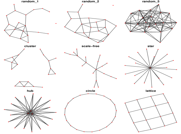
Figure 6: The $9$ different types of undirected graphs for $p=20$, as a number of nodes. For the case graph is Lattice $p=16$. The graphs Random_1, Random_2, Random_5 are random graphs with edge probabilites equal to $0.1$, $0.2$, and $0.5$ respectively ranging from sparse to dense graphs.

While it is straightforward to evaluate $I_{1/2,\mbox{MC}}$, it is less obvious how to compute $I_{1/2,\mbox{Gamm}}$ using Equation 20. The pseudo-code for evaluating the $I_{1/2,\mbox{Gamm}}$ is given in Section F of the Supplementary file. We represent the boxplot of the numerical values of $I_{1/2,\mbox{MC}}$ and $I_{1/2,\mbox{Gamm}}$ obtained over $100$ replications for nine different types of graphs (Figure 6) along with three different numbers of nodes $p=\{10,20,30\}$ and two different values for $\delta=\{3,10\}$. Besides, we report the corresponding values of $v_{D}$ so that one can see the variation of the accuracy of $I_{1/2,\mbox{Gamm}}$, as $v_{D}$ varies, as predicted by Theorem 2, but also that of $I_{1/2,\mbox{MC}}$.

For the case $\delta=3$, the values of $I_{1/2,\mbox{MC}}$ and $I_{1/2,\mbox{Gamm}}$ are represented in Figure 7 for $p=20$, and Figures 10 and 11 in Section G of the Supplementary File for $p=\{10,30\}$. We see that the values of $I_{1}/I_{2}$ slightly move away from 1 as $v_{D}$ moves away from 0. But in all cases, we see that $I_{1/2,\mbox{MC}}$ and $I_{1/2,\mbox{Gamm}}$ cover the same range of values and their medians are between $0.9$ and 1, giving relative errors less than $0.10$. While, from these facts, we cannot immediately conclude that the assumption of $v_{D}$ small is always satisfied, it is a strong indication that it is satisfied enough to ensure that our approximation is acceptable.

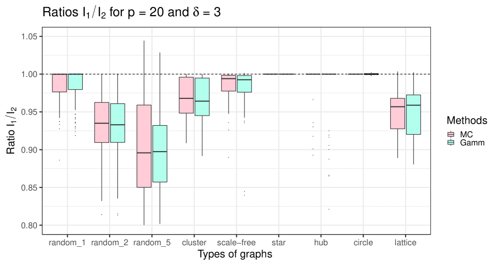
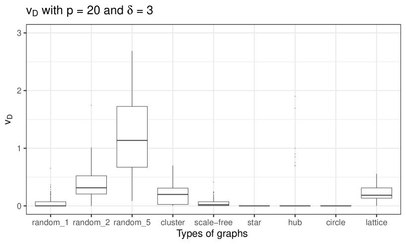
Figure 7: (Top) The boxplot for the ratio $I_{1}/I_{2}$ computed by the MC approach of Atay-Kayis and Massam (2005) (in red) and our approximation (20) (in blue). (Bottom) The boxplot of the variance $v_{D}$ of $b_{1}$ for the corresponding graphs. These computations are done over 100 replications for nine different graphs (Figure 6) with $p=20$ nodes and $\delta=3$.

For the case $\delta=10$, the values of $I_{1/2,\mbox{MC}}$ and $I_{1/2,\mbox{Gamm}}$ are represented in Figure 8 for $p=20$, and Figures 12 and 13 for $p=\{10,30\}$ in Section G of the Supplementary File. In all cases, we see that $I_{1/2,\mbox{MC}}$ and $I_{1/2,\mbox{Gamm}}$ cover the same range of values and their medians are between $0.995$ and 1, giving pretty low relative errors of less than $0.005$.

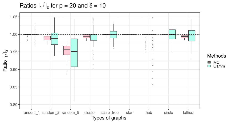
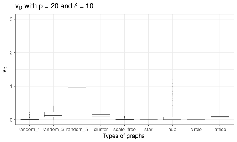
Figure 8: (Top) The boxplot for the ratio $I_{1}/I_{2}$ computed by the MC approach of Atay-Kayis and Massam (2005) (in red) and our approximation (20) (in blue). (Bottom) The boxplot of the variance $v_{D}$ of $b_{1}$ for the corresponding graphs. These computations are done over 100 replications for nine different graphs (Figure 6) with $p=20$ nodes and $\delta=10$.

We verify this result numerically. Besides, our numerical results show our approximation $I_{1}/I_{2}$ (given by $I_{1/2,\mbox{Gamm}}$) is accurate (close to 1) even for the cases that $v_{D}$’s are not close to $0$. In fact, both set of values for $I_{1/2,\mbox{MC}}$ and $I_{1/2,\mbox{Gamm}}$ seem to be affected by the size of $v_{D}$ but are reasonably close to 1, whatever the value of $v_{D}$.

We should mention that our simulations indicate that our approximation is more accurate for the sparser graphs. For example, in Figure 7 (top) consider the graphs Random_1, Random_2, and Random_5 which are respectively ranging from sparse to dense graphs. This figure as well as the other figures in this section indicate that our approximation is more accurate for the sparser graphs.

For $p>30$, we cannot verify the accuracy of our approximation directly by computing $I_{1/2,\mbox{MC}}$ and $I_{1/2,\mbox{Gamm}}$ because of the limitations of the Monte Carlo method of Atay-Kayis and Massam (2005). So, in the next section, for graphs with up to $150$ nodes, we will verify the performance of our approximation in the search algorithm that represents in Section 2.1.

6 Simulation study for high-dimensional graphs

We perform Bayesian structure learning on simulated data from high-dimensional graphs using the BDMCMC search algorithm, represented in Algorithm 1. We use our approximation (8) within Algorithm 1 and we call it BDMCMC-Gamm. For the sake of comparison, we also evaluate the ratio of normalizing constants, within the BDMCMC search algorithm, using the exchange algorithm which is represented in Algorithm 2, we call it BDMCMC-DMH; This algorithm can be considered as the state-of-the-art. Both approaches are implemented in the BDgraph R package (Mohammadi and Wit, 2019a, b) in the function bdgraph().

We consider four following graph structures:

• Scale-free: A graph which has a power-law degree distribution generated by the Barabási-Albert algorithm (Albert and Barabási, 2002).

• Random_p: A graph in which edges are randomly generated from independent Bernoulli distributions with mean equal to $p$.

• Random_2p: The same as the Random_p graph with mean equal to $2p$.

• Cluster: A graph in which the number of clusters is $\left|p/20\right|$. Each cluster has the same structure as the Random_p graph.

For each graph, we consider various scenarios based on the number of nodes $p\in\{50,100,150\}$ and the sample size $n\in\{p,2p\}$. We draw $n$ independent samples from the normal $N_{p}(0,K)$ distribution. We consider $\delta=3$, which is the worst-case value for our approximation (see subsections 4.1 and 5.1).

For each scenario, we run Algorithm 1 by using our approximation (8) as well as Algorithm 2 which is based on an exchange algorithm. The number of iterations is $100,000$ with $60,000$ iterations as burn-in. To evaluate the performance of both algorithms we use ROC curves, based on model averaging, by computing true and false-positive rates for each of $50$ replicated data sets and then by averaging over the $50$ replicates.

Figure 9 represents the ROC curves for the cases $p=150$ with $n\in\{150,300\}$. The ROC curves for $p=50$ and $p=100$ are, respectively, in Figures 14 and 15 in Section G of the Supplementary File. As we can see, in almost all cases, the performance of the BDMCMC algorithm based on both approximations is the same. In a few cases, the BDMCMC algorithm using our approximation (8) performs slightly better than the BDMCMC algorithm using the exchange algorithm: this happens especially when $p$ is large, for example, when $p=150$ and $n=150$. This discrepancy can be due to the convergence issue of the exchange algorithm in high-dimensional graphs.

The execution times for both algorithms are represented on the right-hand side of Figure 1. It indicates the computational gain of using our approximation within the search algorithm. For example, in the case $p=150$, the BDMCMC algorithm using our approximation is more than $3$ times faster than the BDMCMC algorithm using the exchange algorithm.

In summary, our simulation study shows that, from an accuracy point of view, the BDMCMC algorithm using our approximation (8), performs well especially for high-dimensional sparse graphs, which is the case for many real-world applications. From a computational point of view, using our approximation speeds up the BDMCMC search algorithm for the models with high-dimensional graphs.

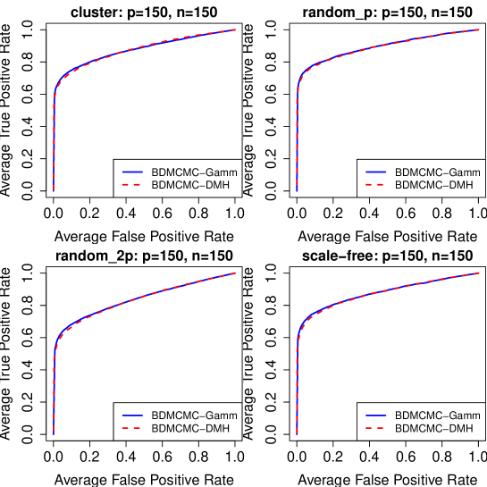
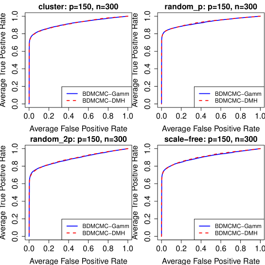
Figure 9: ROC curves for the BDMCMC algorithm with our approximation (8) (BDMCMC-Gamm) and BDMCMC algorithm with exchange algorithm (BDMCMC-DMH), over $50$ replications. Here, $p=150$, $n\in\{150,300\}$, and $4$ different graph structures.

7 Conclusion

In this paper, we represent a search algorithm in which the the prior normalizing constants of G-Wishart is carried out by our approximation in Equation 8. Using our approximation allows for Bayesian structure learning to avoid the sampling-based methods as computationally expensive updates within the search algorithm. We give theoretical results to justify this approximation when certain assumptions are satisfied. Then, as importantly, we show, through numerical experiments that the assumptions are reasonably satisfied and yield a good accuracy of the approximation. In Theorem 1, we consider the specific case where the paths between the endpoints are disjoint. Though this case is unrealistic in practice of course, it is interesting because we can obtain an analytic lower bound to the ratio $I_{1}/I_{2}$, which is a function of $\delta$ and the number of paths and their length. We see that the actual accuracy is much better than that given by the lower bound.

In the realistic and general case where the paths are not necessarily disjoint, we give an alternative expression in Theorem 2 for the ratio $I_{1}/I_{2}$, then an approximation to this expression. We show that when the variance $v_{D}$ is small, then the accuracy is good. When performing structure learning in practice, one will not verify this assumption any more than one would verify that the paths are disjoint. But we do examine a large array of standard graphs and verify numerically that the assumption of $v_{D}$ small is satisfied in most cases. Whatever the value of $v_{D}$, the accuracy of the approximation $I_{1}/I_{2}\approx 1$, or equivalently of the approximation in Equation 8, is very good. We do so by direct computation for graphs of size $p\leq 30$. Due to the limitations of Monte Carlo method to compute $I_{1}/I_{2}$, we cannot perform these direct computations for $p>30$. In that case, we perform structure learning on graphical models with up to $150$ variables and obtain the good results of Section 6. We should emphasize here that we stopped at $p=150$ because, beyond this size, the state-of-the-art algorithms become computationally expensive but the BDMCMC search algorithm with our approximation (8) can scale up to higher dimensions still.

The accuracy of our approximation (8) depends on (i) the value of $\delta$ (scale parameter of G-Wishart) (ii) the structure of the graphs, more specifically its sparsity. We illustrate it in the simulations of Sections 4.1 and 5.1. It also can be interpreted from Theorems 1 and 2. The accuracy of our approximation is increased by increasing the values of $\delta$. Thus, our recommendation in practice is to choose, preferably, the value of $\delta$ higher than $10$, to be on the save side. For the case of graph structure, the accuracy of our approximation depends on the sparsity of the graphs. Our results indicated that our approximation is more accurate for the sparser graphs, as is indicated in the simulations of Section 5.1. Since in real-life applications the underlying graphs are not dense (mainly sparse) is safe to use our approximation in practice.

In conclusion, we think that our approximation can be safely adopted in the search algorithm to replace the sampling-based methods such as the exchange algorithm. Finally, we also proved that $I_{1}/I_{2}\leq 1$. It shows that our approximation (8) yields a Bayes factor which favours $G^{-e}$ compared to $G$ so that we know that a model search using our approximation might lead to sparser graphs.

SUPPLEMENTARY MATERIALS

The supplementary materials contain technical proofs for all the theorems from the main article as well as additional simulation results.

Appendix A Proposition

The following proposition is used to compute $\mathbb{E}\left(e^{-\frac{A^{2}}{2}}\right)$ where $A$ defined in Equation 11 of the manuscript.

Proposition 2.

Let $U_{1},\ldots,U_{k}$, $V_{1}\dots,V_{k}$, and $Q$ be independent random variables such that $U_{i}$ and $V_{i}$ are $N(0,1)$ and $Q\sim\chi^{2}_{\delta}$. Then

$$E\left(e^{-\frac{1}{2Q}\left(\sum_{i=1}^{k}U_{i}V_{i}\right)^{2}}\right)=\frac{\Gamma\left(\frac{\delta+k}{2}\right)\Gamma\left(\frac{\delta+1}{2}\right)}{\Gamma\left(\frac{\delta}{2}\right)\Gamma\left(\frac{\delta+k+1}{2}\right)}.$$

Proof. We have

$$\sum_{i=1}^{k}U_{i}V_{i}\sim\left(U_{1}^{2}+\cdots+U_{k}^{2}\right)^{\frac{1}{2}}V_{1}=X^{\frac{1}{2}}V_{1},$$ (21)

where $X\sim\Gamma(\frac{k}{2},\frac{1}{2})$; To see this, we compute the Laplace transforms of both sides as follow

$$E\left(e^{-\frac{1}{2Q}\left(\sum_{i=1}^{k}U_{i}V_{i}\right)^{2}}\right)=E\left(e^{\frac{X}{Q}\frac{-V_{1}}{2}}\right)=E\left(\left(1+\frac{X}{Q}\right)^{\frac{-1}{2}}\right),$$

where the last equality is due to integrating with regard to variable $V_{1}$. Since $X\sim\Gamma(\frac{k}{2},\frac{1}{2})$ and $Q\sim\Gamma(\frac{d}{2},\frac{1}{2})$, we have $U=\frac{X}{Q}\sim B_{2}\left(\frac{k}{2},\frac{d}{2}\right)$ which is a Beta distribution of second kind. Thus

$$E\left(\left(1+\frac{X}{Q}\right)^{\frac{-1}{2}}\right)=\frac{\Gamma\left(\frac{\delta+k}{2}\right)\Gamma\left(\frac{\delta+1}{2}\right)}{\Gamma\left(\frac{\delta}{2}\right)\Gamma\left(\frac{\delta+k+1}{2}\right)}.$$

Appendix B Proof of Lemma 1

By considering $\Psi_{\cap}^{-}=\left\{\psi_{ij}:(i,j)\in E\setminus\left(E_{q}\cap E_{p}\right)\right\}$, we have

$$\mathbb{E}\left(e^{-\frac{D}{2}-\frac{(A+b)^{2}}{2}}\right)=\mathbb{E}\left(e^{-\frac{D}{2}}\mathbb{E}\left(e^{-\frac{(A+b)^{2}}{2}}\big{|}\Psi_{\cap}^{-}\right)\right).$$

Note that $D$ and $b_{1}$ are $\Psi_{\cap}^{-}$-measurable, that is, are functions of the elements of $\Psi_{\cap}^{-}$ only. Due to Equation 21, we have

$$\mathbb{E}\left(e^{\frac{-(A_{1}+b_{1})^{2}}{2\psi_{qq}}}\big{|}\Psi_{\cap}^{-}\right)=\mathbb{E}\left(e^{-\frac{1}{2}\,\frac{(UV+b_{1})^{2}}{\psi_{qq}}}\big{|}\Psi_{\cap}^{-}\right)$$

where $U$, $V$, and $\psi_{qq}$ are independent random variables such that $U^{2}\sim\chi^{2}_{d}$, $V\sim N(0,1)$, and $\psi_{qq}\sim\chi^{2}_{\delta}$. Integrating with respect to $V\sim N(0,1)$, we obtain

$$\mathbb{E}\left(e^{-\frac{1}{2}\,\frac{(UV+b_{1})^{2}}{\psi_{qq}}}\big{|}\Psi_{\cap}^{-}\right) =\mathbb{E}\left(e^{-\frac{1}{2}\,\frac{b_{1}^{2}}{U^{2}+\psi_{qq}}}\left(\frac{\psi_{qq}}{U^{2}+\psi_{qq}}\right)^{\frac{1}{2}}\Big{|}\Psi_{\cap}^{-}\right)$$

$$=\mathbb{E}\left(\sqrt{B}\right)\mathbb{E}\left(e^{\frac{-b_{1}^{2}}{2Y}}\big{|}\Psi_{\cap}^{-}\right),$$

where $B=\frac{\psi_{qq}}{U^{2}+\psi_{qq}}\sim Beta({\frac{\delta}{2},\frac{d}{2}})$ and is independent of $Y=U^{2}+\psi_{qq}\sim\chi^{2}_{\delta+d}$. Thus

$$\mathbb{E}\left(\sqrt{B}\right)=\frac{\Gamma(\frac{\delta+1}{2})\Gamma(\frac{\delta+d}{2})}{\Gamma(\frac{\delta+d+1}{2})\Gamma(\frac{\delta}{2})},$$

which is equal to $\mathbb{E}\left(e^{-\frac{A^{2}}{2}}\right)$. Since $Y\sim\chi_{\delta+d}^{2}$, we have

$$\mathbb{E}\left(e^{\frac{-b_{1}^{2}}{2Y}}\big{|}\Psi_{\cap}^{-}\right)=\mathbb{E}\left(h(b_{1},\delta^{*})\mid\Psi_{\cap}^{-}\right).$$

Regarding that $\Psi_{\cup}^{-}\subset\Psi_{\cap}^{-}$ we have

$$\mathbb{E}\left(h(b_{1},\delta^{*})\mid\Psi_{\cap}^{-}\right)=\mathbb{E}\left(h(b_{1},\delta^{*})\mid\Psi_{\cup}^{-}\right).$$

Note that, while $b_{1}$ is $\Psi_{\cap}^{-}$-measurable, it is not $\Psi_{\cup}^{-}$-measurable.

Appendix C Proof of Lemma 2

We note three important facts. First, the elements of the first row of the matrix $\psi$ are all zero except for those corresponding to the edges of the path $\lambda_{1}$, i.e.

$$\psi_{1v}=0,\;\;\text{for}\;\;v\in\cup_{\lambda\in\Lambda}V_{\lambda}\;\;\text{and}\;\;v\not=\{1,2,q\}.$$

Second, based on the above fact and Equation 10 of the manuscript, the remaining non-free entries in all the columns of $\psi$ except for the columns $q$ and $p$, are equal to zero. Third, due to the first entry $\psi_{1q}$ of column $q$ being free, none of the entries of column $q$ are necessarily zero. However, for each $\lambda\in\Lambda$, using iteratively Equation 10 of the manuscript, we see the non-free entries of column $p$ are zero except for the last one $\psi_{qp}$. Considering these important facts and applying Equation 10 of the manuscript yields

$$\psi_{qp}=\frac{-1}{\psi_{qq}}\sum_{\lambda\in\Lambda}\sum_{i_{\lambda\in V_{\Lambda}}}\psi_{i_{\lambda}q}\psi_{i_{\lambda}p}=\frac{-1}{\psi_{qq}}\sum_{\lambda\in\Lambda}\psi_{\ell_{\lambda}q}\psi_{\ell_{\lambda}p}.$$ (22)

The entries $\psi_{\ell_{\lambda}p},\;\lambda\in\Lambda$ are free. The entries $\psi_{\ell_{\lambda}q}$ are obtained by successively applying Equation 10 of the manuscript and the fact that $\psi_{(j-1)_{\lambda}j_{\lambda}}$, $j=\{1,\ldots,(l-1)\}$ are free and the non-free entries of $\Psi$ are equal to zero expect for the columns $q$ and $p$. That is

$$\begin{split}\psi_{\ell_{\lambda}q}&=-\frac{\psi_{(\ell-1)_{\lambda}\ell_{\lambda}}\psi_{(\ell-1)_{\lambda}q}}{\psi_{(\ell-1)_{\lambda}(\ell-1)_{\lambda}}}=+\frac{\psi_{(\ell-1)_{\lambda}\ell_{\lambda}}\psi_{(\ell-2)_{\lambda}\ell_{\lambda}}\psi_{(\ell-2)_{\lambda}q}}{\psi_{(l-1)_{\lambda}(l-1)_{\lambda}}\psi_{(l-2)_{\lambda}(l-2)_{\lambda}}}\\ &=\ldots\\ &=(-1)^{\ell_{\lambda}-1}\frac{\psi_{1_{\lambda}q}\prod_{j=1}^{\ell-1}\psi_{j_{\lambda}(j+1)_{\lambda}}}{\prod_{j=2}^{\ell}\psi_{j_{\lambda}j_{\lambda}}}=(-1)^{\ell_{\lambda}-1}\frac{\psi_{1_{\lambda}q}\prod_{j=1}^{\ell-1}\psi_{j_{\lambda}(j+1)_{\lambda}}}{\prod_{j=1}^{\ell-1}\psi_{(j+1)_{\lambda}(j+1)_{\lambda}}},\\ &=(-1)^{\ell_{\lambda}-1}\psi_{1_{\lambda}q}\prod_{j=1}^{l-1}\frac{\psi_{j_{\lambda}(j+1)_{\lambda}}}{\psi_{(j+1)_{\lambda}(j+1)_{\lambda}}}.\end{split}$$

Above equality and Equation 22 together yield

$$\psi_{qp}=\frac{1}{\psi_{qq}}\sum_{\lambda\in\Lambda}(-1)^{\ell_{\lambda}}\frac{\psi_{1_{\lambda},q}\psi_{\ell_{\lambda},p}\prod_{j=1}^{\ell-1}\psi_{j_{\lambda},(j+1)_{\lambda}}}{\prod_{j=2}^{l}\psi_{j_{\lambda},j_{\lambda}}}=\frac{1}{\psi_{qq}}\sum_{\lambda\in\Lambda}(-1)^{\ell_{\lambda}}\psi_{\ell_{\lambda},p}\psi_{1_{\lambda},q}\prod_{j=1}^{\ell-1}\frac{\psi_{j_{\lambda},(j+1)_{\lambda}}}{\psi_{(j+1)_{\lambda},(j+1)_{\lambda}}},$$

which is identical to Equation 17 of the manuscript.

Appendix D Proof of Theorem 1

The proof relies on a fact that for the case where the paths between $q$ and $p$ are disjoint, we rewrite $A_{1}$ and $b_{1}$ in Equations 11 and 12 of the manuscript as

$$A_{1}=\sum_{\lambda\in\Lambda,l_{\lambda=1}}\psi_{\ell_{\lambda},q}\psi_{\ell_{\lambda},p},\;\;\;b_{1}=\sum_{\lambda\in\Lambda,\ell_{\lambda}\geq 2}b_{1\lambda},$$

where

$$b_{1\lambda}=(-1)^{\ell_{\lambda}}\psi_{1_{\lambda},q}\psi_{\ell_{\lambda},p}\prod_{j_{\lambda}=1}^{\ell_{\lambda}-1}\frac{\psi_{j_{\lambda},(j+1)_{\lambda}}}{\psi_{(j+1)_{\lambda},(j+1)_{\lambda}}}$$

with the convention that $b_{1\lambda}=0$ if $\ell_{\lambda}=1$, and

$$D=\sum_{\lambda\in\Lambda}D_{\lambda}\;\text{ where }\;\;D_{\lambda}=\sum_{k=2}^{\ell_{\lambda}}\left((-1)^{k-1}\psi_{1_{\lambda},q}\prod_{j_{\lambda}=1}^{k-1}\frac{\psi_{j_{\lambda},(j+1)_{\lambda}}}{\psi_{(j+1)_{\lambda},(j+1)_{\lambda}}}\right)^{2}.$$

All the entries appearing in the expression for $A_{1}$ and $b_{1}$ are free variables independent of each other and those appearing in $b_{1\lambda},\lambda\in\Lambda,\ell_{\lambda}\geq 2$ are different from those appearing in $A_{1}$. Thus, $A_{1}$ and $\sum_{\lambda\in\Lambda,\ell_{\lambda}\geq 2}b_{1\lambda}$ are stochastically independent. Moreover, according to Proposition 1, all $\psi_{ij},i\not=j$ are $N(0,1)$ random variables while $\psi_{ii}^{2}$ follow a $\chi^{2}_{\delta+\nu_{i}}$ distribution. In particular $\psi^{2}_{qq}\sim\chi^{2}_{\delta}$.

To find a lower bound for the $I_{1}/I_{2}$, we use the Gaussian equality as follows: if $Z\sim N(0,\sigma^{2})$, then

$$\mathbb{E}\left(e^{itZ}\right)=\int_{-\infty}^{+\infty}e^{itz}e^{-\frac{z^{2}}{2\sigma^{2}}}\frac{dz}{\sigma\sqrt{2\pi}}=e^{-\frac{\sigma^{2}t^{2}}{2}}.$$

Applying above equality with $t=b_{1}$ and $\sigma^{2}=\frac{1}{y}$, we have

$$h(b_{1},\delta^{*}) = \frac{2^{-\delta^{*}}}{\Gamma(\delta^{*})}\int_{0}^{+\infty}y^{\delta^{*}-1}e^{\frac{-y}{2}}e^{\frac{-b_{1}^{2}}{2y}}dy$$

$$= \frac{2^{-\delta^{*}}}{\Gamma(\delta^{*})}\int_{0}^{+\infty}y^{\delta^{*}-1}e^{\frac{-y}{2}}\left(\int_{-\infty}^{+\infty}e^{ib_{1}z}e^{-\frac{yz^{2}}{2}}\sqrt{y}\frac{dz}{\sqrt{2\pi}}\right)dy$$

$$= \frac{2^{-\delta^{*}}}{\Gamma(\delta^{*})\sqrt{2\pi}}\int_{+\infty}^{+\infty}e^{ib_{1}z}\left(\int_{0}^{+\infty}y^{\delta^{*}-1/2}e^{\frac{-(1+z^{2})y}{2}}dy\right)dz$$

$$= \frac{2^{-\delta^{*}}}{\Gamma(\delta^{*})\sqrt{2\pi}}\int_{+\infty}^{+\infty}e^{ib_{1}z}\left(\frac{\Gamma(\delta^{*}+1/2)}{\left(\frac{1+z^{2}}{2}\right)^{\delta^{*}+1/2}}\right)dz$$

$$= \int_{+\infty}^{+\infty}e^{ib_{1}z}f(z)dz,$$

where

$$f(z)=\frac{\Gamma(\delta^{*}+1/2)}{\sqrt{\pi}\Gamma(\delta^{*})}\left(1+z^{2}\right)^{-\delta^{*}+1/2}.$$

Thus

$$\begin{split}\mathbb{E}\left(e^{-\frac{D}{2}}\mathbb{E}\left(h(b_{1},\delta^{*})\mid\Psi_{\cup}^{-}\right)\right)&=\int_{+\infty}^{+\infty}\mathbb{E}\left(e^{-\frac{D}{2}+ib_{1}z}\right)f(z)dz\\ &=\prod_{\lambda\in\Lambda}\int_{+\infty}^{+\infty}\mathbb{E}\left(e^{-\frac{D_{\lambda}}{2}+ib_{1\lambda}z}\right)f(z)dz\end{split}.$$

Similarly, we have

$$\mathbb{E}\left(e^{-\frac{D}{2}}\right)=\prod_{\lambda\in\Lambda}\mathbb{E}\left(e^{-\frac{D_{\lambda}}{2}}\right).$$

Consider independent identically distributed random variables $X_{1},\ldots,X_{n},\ldots$ such that $X_{1}\sim Z/\sqrt{Q}$ with $Z\sim N(0,1)$ independent of $Q\sim\chi^{2}_{\delta+1}$. For $\ell=\ell_{\lambda},\lambda\in\Lambda$, we define

$$S_{\ell}=X_{1}^{2}+X_{1}^{2}X_{2}^{2}+\cdots+(X_{1}\ldots X_{\ell-1})^{2},\ \ B_{\ell}=X_{1}X_{2}\ldots X_{\ell-1}.$$ (23)

We see that for $\lambda\in\Lambda$, we have

$$D_{\lambda} \sim N_{1_{\lambda}q}S_{\ell_{\lambda}},$$

$$b_{1\lambda} \sim N_{1_{\lambda}q}N_{\ell_{\lambda}p}B_{\ell_{\lambda}},$$

where $N_{1_{\lambda}q}$ and $N_{\ell_{\lambda}p}$ are independent $N(0,1)$ random variables, independent of $X_{1},\ldots,X_{\ell},\ldots$. We note that, from the independence of the entries of $\psi_{E}$, we have

$$(b_{1\lambda},D_{\lambda},N_{1_{\lambda}q},N_{\ell_{\lambda}p}),\;\;\;\lambda\in\Lambda$$

are mutually independent.

Omitting the index $\lambda$ on $\ell_{\lambda}$, and simplifying $N_{1_{\lambda}q}$ to $N_{q}$ and $N_{\ell_{\lambda}p}$ to $N_{p}$, we define

$$g_{\ell}(x)=\mathbb{E}\left(e^{-\frac{N_{q}^{2}S_{\ell}}{2}+iN_{p}N_{q}B_{\ell}x}\right).$$

Then

$$I_{1}=\prod_{\lambda\in\Lambda}\int_{-\infty}^{\infty}g_{\ell_{\lambda}}(x)f(x)dx\;\;\text{ and }\;\;I_{2}=\prod_{\lambda\in\Lambda}g_{\ell_{\lambda}}(0).$$

Therefore we can write

$$\begin{split}\frac{I_{2}-I_{1}}{I_{2}}&=\int_{-\infty}^{\infty}\frac{\prod_{\lambda\in\Lambda}g_{\ell_{\lambda}}(0)-\prod_{\lambda\in\Lambda}g_{\ell_{\lambda}}(x)}{\prod_{\lambda\in\Lambda}g_{\ell_{\lambda}}(0)}f(x)dx\\ &\leq\int_{-\infty}^{\infty}\sum_{\lambda\in\Lambda}\frac{g_{\ell_{\lambda}}(0)-g_{\ell_{\lambda}}(x)}{g_{\ell_{\lambda}}(0)}f(x)dx,\end{split}$$ (24)

where the last inequality is based on Lemma 4 applied to $a_{\lambda}=g_{\ell_{\lambda}}(0)$ and $b_{\lambda}=g_{\ell_{\lambda}}(x)$. Writing $\ell$ for $\ell_{\lambda}$, we have

$$g_{\ell}(0)-g_{\ell}(x) = \mathbb{E}\left(e^{-\frac{N_{q}^{2}S_{\ell}}{2}}\left(1-e^{iN_{p}N_{q}B_{\ell}x}\right)\right)$$

$$\leq \mathbb{E}\left(e^{-\frac{N_{q}^{2}S_{\ell}}{2}}|N_{p}N_{q}X_{1}\ldots X_{\ell-1}|\right)|x|$$

$$\leq \mathbb{E}\left(e^{-\frac{N_{q}^{2}X_{1}^{2}}{2}}|N_{q}X_{1}|\right)\mathbb{E}\left(|N_{p}X_{2}\ldots X_{\ell-1}|\right)|x|$$

$$= \frac{2}{\pi}\frac{\delta}{\delta+2}r(\delta)^{\ell}\;|x|,$$

where the first inequality is due to the fact that $|1-e^{iN_{p}N_{q}B_{\ell}x}|\leq|N_{p}N_{q}B_{\ell}|\;|x|$, the second inequality is due to the fact that $X_{1}^{2}\leq S_{\ell}$ and the independence of $(N_{q},X_{1})$ and $(N_{p},X_{2},\ldots,X_{\ell-1})$, and the last equality is obtained using Equations 25 and 26. Moreover, by using Equation 27, we have

$$\frac{g_{\ell}(0)-g_{\ell}(x)}{g_{\ell}(0)} \leq \frac{\delta^{2}}{\pi(\delta+2)}\left[\frac{\Gamma(\frac{\delta}{2})}{\Gamma(\frac{\delta+1}{2})}\right]^{2}r(\delta)^{\ell}\;|x|,$$

and Equation 24 yields

$$\begin{split}0\leq\frac{I_{2}-I_{1}}{I_{2}}&\leq\frac{\delta^{2}}{\pi(\delta+2)}\left(\frac{\Gamma(\frac{\delta}{2})}{\Gamma(\frac{\delta+1}{2})}\right)^{2}\left(\sum_{\lambda\in\Lambda}r(\delta)^{\ell_{\lambda}}\right)\int_{-\infty}^{\infty}|x|f(x)dx\\ &\leq\frac{\delta^{2}}{\pi(\delta+2)}\left(\frac{\Gamma(\frac{\delta}{2})}{\Gamma(\frac{\delta+1}{2})}\right)^{2}\left(\sum_{\lambda\in\Lambda}r(\delta)^{\ell_{\lambda}}\right)\frac{\Gamma(\delta^{*}-1/2)}{\sqrt{\pi}\Gamma(\delta^{*})}\\ &=\frac{\delta^{2}}{\pi(\delta+2)}\left(\frac{\Gamma(\frac{\delta}{2})}{\Gamma(\frac{\delta+1}{2})}\right)^{2}\left(\sum_{\lambda\in\Lambda}r(\delta)^{\ell_{\lambda}}\right)r(\delta+d-1)\end{split}$$

which leads to Equation 18 of the manuscript.

The following lemmas are used in the proof of Theorem 1.

Lemma 3.

Let $X_{1},\ldots,X_{\ell-1}$ be independent identically distributed random variables such that $X_{1}\sim Z/\sqrt{Q}$ with $Z\sim N(0,1)$ independent of $Q\sim\chi^{2}_{\delta+1}$ where $\delta\geq 3$. Let $N_{p}$ and $N_{q}$ also be standard normal $N(0,1)$ random variables, mutually independent and independent of $X_{1},\ldots,X_{\ell-1}$. We then have

$$\mathbb{E}\left(e^{-\frac{N_{q}^{2}X_{1}^{2}}{2}}\left|N_{q}X_{1}\right|\right)=\sqrt{\frac{2}{\pi}}\frac{\delta}{\delta+2}r(\delta)$$ (25)

and

$$\mathbb{E}\left(\left|N_{p}X_{1}\ldots X_{\ell-1}\right|\right)=\sqrt{\frac{2}{\pi}}r(\delta)^{\ell-1},$$ (26)

where $r(\delta)=\frac{\Gamma(\frac{\delta}{2})}{\sqrt{\pi}\Gamma(\frac{\delta+1}{2})}$. Let $S_{\ell}$ as defined in Equation 23 then

$$\mathbb{E}\left(e^{-\frac{N_{q}^{2}S_{\ell}}{2}}\right)>\frac{2}{\delta}\left(\frac{\Gamma\left(\frac{\delta+1}{2}\right)}{\Gamma\left(\frac{\delta}{2}\right)}\right)^{2}.$$ (27)

Proof.

For Equation 25, the variable $Y=X_{1}^{2}\sim B_{2}\left(\frac{1}{2},\frac{\delta+1}{2}\right)$ which is a Beta distribution of the second kind. Thus

$$\mathbb{E}\left(e^{-\frac{N_{q}^{2}X_{1}^{2}}{2}}|N_{q}X_{1}|\right) = \mathbb{E}\left(\mathbb{E}\left(e^{-\frac{N_{q}^{2}X_{1}^{2}}{2}}|N_{q}X_{1}|\;\Big{|}X_{1}\right)\right)$$

where

$$\mathbb{E}\left(e^{-\frac{N_{q}^{2}X_{1}^{2}}{2}}|N_{q}X_{1}|\;\Big{|}X_{1}\right) = \frac{|X_{1}|}{\sqrt{2\pi}}\int_{-\infty}^{+\infty}|u|e^{-\frac{(1+X_{1}^{2})}{2}u^{2}}du=\sqrt{\frac{2}{\pi}}\frac{|X_{1}|}{1+X_{1}^{2}}.$$

Thus

$$\mathbb{E}\left(e^{-\frac{N_{q}^{2}X_{1}^{2}}{2}}|N_{q}X_{1}|\right)=\sqrt{\frac{2}{\pi}}\mathbb{E}\left(\frac{|X_{1}|}{1+X_{1}^{2}}\right)=\sqrt{\frac{2}{\pi}}\mathbb{E}\left(\frac{\sqrt{Y}}{1+Y}\right)=\sqrt{\frac{2}{\pi}}\frac{\delta}{\delta+2}r(\delta).$$

For Equation 26, by using the mutual independence of $N_{p}$ and $X_{1},\ldots,X_{\ell-1}$ and the fact that $X_{i}^{2}\sim B_{2}\left(\frac{1}{2},\frac{\delta+1}{2}\right)$ for $i=\{1,\ldots,\ell-1\}$, we have

$$\mathbb{E}\left(|N_{p}X_{1}\ldots X_{\ell-1}|\right)=\mathbb{E}\left(|N_{p}|\right)\mathbb{E}\left(|X_{1}|\right)^{\ell-1}=\frac{\sqrt{2}}{\sqrt{\pi}}\left(\frac{\Gamma(\frac{\delta}{2})}{\sqrt{\pi}\Gamma(\frac{\delta+1}{2})}\right)^{\ell-1}=\sqrt{\frac{2}{\pi}}r(\delta)^{\ell-1}$$

For Equation 27, from Chamayou and Letac (1991, Example 9), if $U\sim B_{2}(a,b)$ for $b>a$ and $V$ are independent. Then $U(1+V)\sim V$ if and only if $V\sim B_{2}(a,b-a)$. One applies this to $U=X_{1}^{2}$, $V=S$, $a=\frac{1}{2}$, and $b=\frac{\delta+1}{2}$ since $S^{\prime}=\sum_{i=2}^{\infty}X_{2}^{2}\ldots X_{i}^{2}\sim S$ and $X_{1}^{2}(1+S^{\prime})=S$. Thus $S\sim B_{2}\left(\frac{1}{2},\frac{\delta}{2}\right)$. Since $S_{\ell}<S$, we have

$$\mathbb{E}\left(e^{-\frac{N_{q}^{2}S_{\ell}}{2}}\right)>\mathbb{E}\left(e^{-\frac{N_{q}^{2}S}{2}}\right)=\frac{2}{\delta}\left(\frac{\Gamma\left(\frac{\delta+1}{2}\right)}{\Gamma\left(\frac{\delta}{2}\right)}\right)^{2}.$$

∎

Lemma 4.

Let $a_{1},\ldots,a_{n}$ and $b_{1},\ldots,b_{n}$ be complex numbers such that $\left|b_{i}\right|\leq\left|a_{i}\right|$, for $i=1,\ldots,n$. Then

$$\left|\prod_{i=1}^{n}a_{i}-\prod_{i=1}^{n}b_{i}\right|\leq\prod_{i=1}^{n}\left|a_{i}\right|\sum_{j=1}^{n}\frac{|a_{j}-b_{j}|}{|a_{j}|}.$$

Proof.

$$\left|a_{1}\ldots a_{n}-b_{1}\ldots b_{n}\right| = |\left(a_{1}\ldots a_{n}-b_{1}a_{2}\ldots a_{n}\right)+\left(b_{1}a_{2}\ldots a_{n}-b_{1}b_{2}a_{3}\ldots a_{n}\right)$$

$$\hskip 85.35826pt+\ldots\ldots+\left(b_{1}\ldots b_{n-1}a_{n}-b_{1}b_{2}\ldots b_{n}\right)|$$

$$\leq \sum_{j=1}^{n}\left|\prod_{i=1}^{j-1}b_{i}\prod_{i=j}^{n}a_{i}-\prod_{i=1}^{j}b_{i}\prod_{i=j+1}^{n}a_{i}\right|=\sum_{j=1}^{n}\left|\prod_{i=1}^{j-1}b_{i}\prod_{i=j+1}^{n}a_{i}\right|\left|a_{j}-b_{j}\right|$$

$$\leq \sum_{j=1}^{n}\left|\prod_{i=1}^{j-1}a_{i}\prod_{i=j+1}^{n}a_{i}\right|\left|a_{j}-b_{j}\right|=\prod_{i=1}^{n}\left|a_{i}\right|\sum_{j=1}^{n}\left|1-\frac{b_{j}}{a_{j}}\right|$$

∎

Appendix E Proof of Theorem 2

The proof of Theorem 2 is long and is done in the next three subsections. In Subsection E.1, we show in Proposition 3 that, conditional on a quantity $\Psi_{\cup}^{-}$ as defined in Equation 15 of the manuscript, $b_{1}$ can be expressed as a bilinear form. In Proposition 4 of Subsection E.2, using its expression as a bilinear form, we show that $b_{1}$ is distributed like the continuous scale mixture of centered Gaussian variables. This allows us to deduce that there exists a unique $v_{D}$ such that the normal $N(0,v_{D})$ distribution best approximates the distribution of $b_{1}$. Finally, in Subsection E.3, we prove Theorem 2: under the assumption that $v_{D}$ is small, $I_{1}/I_{2}$ can accurately be approximated by 1 or equivalently the ratio of the normalizing constants can accurately be approximated by Equation 8 of the manuscript, which is what we want to prove.

E.1 Expression of $b_{1}$ as a bilinear form

Here we want to show that the distribution of $b_{1}$ is a scale mixture of normal distributions which can be approximated by another $N(0,v_{D})$ distribution where the variance $v_{D}$ depends on $\Psi_{\cup}^{-}$. But, to do so, we must first express $b_{1}$ as a bilinear form in two standard normal random vectors.

Regarding $E_{q}=\{(i,j):(i,q)\in E\}$ and $E_{p}=\{(i,j):(i,p)\in E\}$, we define

$$\Psi_{E_{q}^{-}}=\{\psi_{ij}:(i,j)\in E_{q}\setminus E_{p}\},\;\;\;\Psi_{E_{p}^{-}}=\{\psi_{ij}:(i,j)\in E_{p}\setminus E_{q}\}.$$

The $\Psi_{E_{q}^{-}}$ represents the free elements of matrix $\Psi$ regarding to just the neighbor of $q$ and the same for $p$. In the following, we express $D$ and $b_{1}$ as polynomials in $\Psi_{E_{q}^{-}}$ and $\Psi_{E_{p}^{-}}$.

Proposition 3.

Let $N_{q}^{-}$ denote the set of nodes that are neighbours of $q$ but not of $p$ and $N_{p}^{-}$ denote the set of nodes that are neighbours of $p$ but not of $q$. There exist vectors $M_{i}^{q}\in\mathbb{R}^{N_{q}^{-}}$ and $M_{i}^{p}\in\mathbb{R}^{N_{p}^{-}}$, $i=\{1,\ldots,q-d-1\}$, functions of $\Psi_{\cup}^{-}$, such that if $C$ is the $|N_{q}^{-}|\times|N_{p}^{-}|$-dimensional matrix

$$C=\sum_{i=1}^{q-d-1}M^{q}_{i}(M^{p}_{i})^{t}$$

then we have

$$b_{1}=\mbox{tr}\left(\Psi_{E_{q}^{-}}C\Psi_{E_{p}^{-}}\right).$$ (28)

Furthermore, $\left\{M^{q}_{i},M^{p}_{i}\right\}_{i=1}^{q-d-1}$, $\Psi_{E_{q}^{-}}$ and $\Psi_{E_{p}^{-}}$ are independent.

Proof.

From the expression of $b_{1}$ in Equation 12 of the manuscript we have

$$b_{1}=\sum^{q-d-1}_{i=1}\psi_{iq}\psi_{ip},$$

which is based on assume the nodes which are neighbours to both $q$ and $p$, are numbered $q-d,q-d+1,\ldots,p$. By Equation 10 of the manuscript, each $\psi_{iq},(i,q)\in\overline{E}$ is equal to the sum of products

$$\psi_{iq}=\frac{-1}{\psi_{ii}}\sum_{l=1}^{i-1}\psi_{li}\psi_{lq},$$ (29)

where each of these $\psi_{li}$ or $\psi_{lq}$, $l=\{1,\ldots,q-d-1\}$ may be free or not free. If $\psi_{lq}$ is free, $l$ necessarily belongs to $N_{q}^{-}$ because it is a neighbour of $q$ and, since $i\leq q-d$ and $l\leq i$, it cannot be a neighbour of both $q$ and $p$. If it is not free, then, we write the expression of $\psi_{lq}$ according to Equation 10 of the manuscript and we repeat this process until $\psi_{lq}$ has been expressed in terms of a ratio of a product of $\psi_{uv},(u,v)\in E,u\leq l,v\leq q$, one of which is necessarily (since the sum in Equation 29 is finite) equal to $\psi_{u_{l}q}$ for some $u_{l}\leq l,u_{l}\in N_{q}^{-}$, and a product of $\psi_{vv},v\leq l$. Similarly $\psi_{li}$ is free or not free. If not free, it will be expressed as a ratio of products of elements of $\psi_{E}$, none of which, in the numerator, can be equal to $\psi_{u_{l}q}$ since it is the product of entries $\psi_{uv}$ of $\psi$ with $u\leq l,v\leq i<q$. Thus, from Equation 29, we can write, for each $i=\{1,\ldots,q-d-1\}$

$$\psi_{iq}=\frac{-1}{\psi_{ii}}\sum_{l=1}^{i-1}\psi_{li}\psi_{lq}=\sum_{l\in N_{q}^{-}}(M_{i}^{q})_{l}\;\psi_{u_{l},q}=\mbox{tr}\left(M_{i}^{q}\Psi_{E_{q}^{-}}\right),$$ (30)

where $(M_{i}^{q})_{l},l\in N_{q}^{-}$ are the components of $M_{i}^{q}$, some of which can be equal to 0, if the Cholesky equations (in Equation 10 of the manuscript) do not lead to that particular $l\in N_{q}^{-}$, or 1, if $l\in N_{q}^{-}$. Similarly, we have

$$\psi_{ip}=\frac{-1}{\psi_{ii}}\sum_{l=1}^{i-1}\psi_{li}\psi_{lp}=\sum_{l\in N_{p}^{-}}(M_{i}^{p})_{l}\;\psi_{v_{l},p}=\mbox{tr}\left(M_{i}^{p}\Psi_{E_{p}^{-}}\right),$$ (31)

for some $v_{l}<l,v_{l}\in N_{p}^{-}$ and Equation 28 follows from Equations 30 and 31. ∎

Example 2.

Consider the graph in Figure 3 (right) of the manuscript where $q=6$, $p=7$, $N_{q}=\{1,2,5\}$, $N_{p}=\{3,4,5\}$, $N_{q}^{-}=\{1,2\}$, $N_{p}^{-}=\{3,4\}$, $d=1$, and $\psi_{E}=\{\psi_{14},\psi_{16},\psi_{23},\psi_{24},\psi_{26}$, $\psi_{37},\psi_{47},\psi_{56},\psi_{57}\}$. Thus $\Psi_{E_{q}^{-}}=\left(\psi_{16},\psi_{26}\right)$ and $\Psi_{E_{p}^{-}}=\left(\psi_{37},\psi_{47}\right)$. Using the notation $X_{ij}=\psi_{ij}/\psi_{jj}$ for convenience, the non-free entries are

$$\psi_{34} = -\psi_{24}X_{23},$$

$$\psi_{36} = -\psi_{26}X_{23}=-\left(\psi_{16},\psi_{26}\right)\left(0,X_{23}\right)^{t}=\mbox{tr}(\Psi_{E_{q}^{-}}M^{q}_{3}),$$

$$M^{q}_{3} = \left(0,X_{23}\right),$$

$$\psi_{46} = -\psi_{26}X_{23}^{2}X_{24}-\psi_{26}X_{24}-\psi_{16}X_{14}=-\left(\psi_{16},\psi_{26}\right)\left(X_{14},X_{24}+X_{23}^{2}X_{24}\right)^{t}=\mbox{tr}\left(\Psi_{E_{q}^{-}}M^{q}_{4}\right),$$

$$M^{q}_{4} = -\left(X_{14},X_{24}+X_{23}^{2}X_{24}\right)^{t},$$

$$\psi_{67} = \frac{1}{\psi_{66}}\left(-\psi_{57}\psi_{56}+\psi_{26}X_{23}^{2}X_{24}\psi_{47}+\psi_{26}X_{24}\psi_{47}+\psi_{16}X_{14}\psi_{47}+\psi_{26}X_{23}\psi_{37}\right)$$

$$= \frac{1}{\psi_{66}}\left(A_{1}+b_{1}\right),$$

where

$$A_{1} = -\psi_{57}\psi_{56},$$

$$b_{1} = \psi_{26}X_{23}^{2}X_{24}\psi_{47}+\psi_{26}X_{24}\psi_{47}+\psi_{16}X_{14}\psi_{47}+\psi_{26}X_{23}\psi_{37}.$$

It leads $b_{1}=\Psi_{E_{q}^{-}}^{t}C\Psi_{E_{p}^{-}}$ where

$$C=\left[\begin{array}[]{cc}0&X_{14}\\ X_{23}&X_{24}+X_{23}^{2}X_{24}\end{array}\right].$$

It also follows from the definition of $\Psi_{E_{q}^{-}}$ that $M_{1}^{q}=(1,0)^{t}$ and $M_{2}^{q}=(0,1)^{t}$. From the definition of $\Psi_{E_{p}^{-}}$, we have $M_{1}^{p}=M_{2}^{p}=(0,0)^{t}$ and $M_{3}^{p}=(1,0)^{t}$ and $M_{4}^{p}=(0,1)^{t}$. We can then verify

$$\mbox{tr}\left(\Psi_{E_{q}^{-}}^{t}C\Psi_{E_{p}^{-}}\right)=\sum_{i=1}^{4}\mbox{tr}\left(\Psi_{E_{q}^{-}}M_{i}^{q}\right)\mbox{tr}\left(\Psi_{E_{p}^{-}}M_{i}^{p}\right).$$

E.2 A normal approximation to the distribution of $b_{1}$

We see in Equation 28, that if we condition on $\Psi_{\cup}^{-}$, as defined in Equation 15 of the manuscript, then $b_{1}$ can be expressed as the bilinear form of $\Psi_{E_{q}^{-}}$ and $\Psi_{E_{p}^{-}}$ as

$$b_{1}=\Psi_{E_{q}^{-}}^{t}C\Psi_{E_{p}^{-}},$$

where $C=\sum_{i=1}^{q-d-1}(M^{q}_{i})^{t}M_{i}^{p}$ is a matrix of rank $m\leq\min\left(|N_{q}^{-}|,|N_{p}^{-}|\right)$. Once $\Psi_{\cup}^{-}$ is known, $C$ is fixed. We are now going to show that, conditional on $\Psi_{\cup}^{-}$, the distribution of $b_{1}$ has the following property.

Proposition 4.

When conditioned by $\Psi_{\cup}^{-}$, the distribution of $b_{1}$ is a continuous scale mixture of centered normal distributions. More precisely, $b_{1}$ follows the same distribution as $X\sqrt{Y/2}$ where $X$ and $Y$ are independent with $X\sim N(0,1)$ and

$$Y=\sum_{i=1}^{m}\frac{Y_{i}}{\lambda_{i}}\;\;\text{ where }\;\;Y_{i}\stackrel{{\scriptstyle iid}}{{\sim}}\chi_{2}^{2}$$

and where $1/\lambda_{1},\ldots,1/\lambda_{m}$ are the non-zero eigenvalues of $C^{T}C.$

Proof.

We first show that $b_{1}$ follows the same distribution as $X\sqrt{Y/2}$. To do so, it suffices to show the two Laplace transforms $\mathbb{E}\left(e^{sb_{1}}\right)$ and $\mathbb{E}\left(e^{sX\sqrt{Y/2}}\right)$ coincide. Integrating this last expected value first with respect to $X$, holding $Y$ fixed, and then with respect to $Y$, we obtain

$$\mathbb{E}\left(e^{sX\sqrt{Y/2}}\right)=\mathbb{E}\left(e^{s^{2}Y/2}\right)=\prod_{j=1}^{m}\left(1-\frac{\lambda_{j}s^{2}}{2}\right)^{\frac{-1}{2}}.$$

Next, from Equation 28 and then integrating with respect to $\Psi_{E_{q}^{-}}$, we have

$$\mathbb{E}\left(e^{sb_{1}}\right)=\mathbb{E}\left(e^{s\mbox{tr}\left(\Psi_{E_{q}^{-}}C\Psi_{E_{p}^{-}}\right)}\right)=\mathbb{E}\left(e^{\frac{s^{2}}{2}\mbox{tr}\left(\Psi_{E_{p}^{-}}C^{t}C\Psi_{E_{p}^{-}}\right)}\right).$$

Now we have

$$\mbox{tr}\left(\Psi_{E_{p}^{-}}C^{t}C\Psi_{E_{p}^{-}}\right)\sim Z^{t}\mathrm{diag}(1/\lambda_{1},\ldots,1/\lambda_{m})Z,$$

where $Z=(Z_{1},\ldots,Z_{m})$ are independent $N(0,1)$ random variables. Thus $b_{1}$ and $X\sqrt{Y/2}$ have the same Laplace transform. ∎

To show the distribution of $b_{1}$ is a scale mixture of centered normals, we note that if $X\sim N(0,1)$ and $V=Y/2$ is any positive random variable with distribution $\mu(dv)$, then if $U=X\sqrt{Y/2}$, the density of $U$ is

$$f_{U}(u)=\int_{0}^{+\infty}\frac{e^{-\frac{u^{2}}{2v}}}{\sqrt{2\pi v}}\mu(dv).$$

So, the distribution of $U$, that is the distribution of $b_{1}$, is a mixture of normal $N(0,v)$ distributions. Following Letac and Massam (2020, Theorem 3.1.), with the distribution of $b_{1}$ for $f$, we deduce that there exists a unique $v_{D}$ such that the normal $N(0,v_{D})$ distribution best approximates the distribution of $b_{1}$.

E.3 Expression $I_{1}/I_{2}$ regarding $b_{1}\sim N(0,v_{D})$

We will now derive an expression for $I_{1}/I_{2}$ when we approximate the distribution of $b_{1}$ by the $N(0,v_{D})$ distribution. We start with the following lemma.

Lemma 5.

Under the approximation $b_{1}\sim N(0,v_{D})$, we have

$$\mathbb{E}\left(h(b_{1},\delta^{*})\big{|}\Psi_{\cup}^{-}\right)=\frac{v_{D}^{\delta^{*}}}{2^{\delta^{*}}\Gamma(\delta^{*})}\int_{0}^{\infty}t^{\delta^{*}-\frac{1}{2}}(1+t)^{\frac{-1}{2}}e^{-\frac{v_{D}t}{2}}dt,$$

where $\delta^{*}=\frac{\delta+d}{2}$ and $h(b_{1},\delta^{*})$ defined in Equation 14 of the manuscript. Moreover, when $v_{D}$ is small, we have

$$\mathbb{E}\left(h(b_{1},\delta^{*})\big{|}\Psi_{\cup}^{-}\right)=1-\frac{\Gamma(\delta^{*}+\frac{1}{2})}{\Gamma(\delta^{*})}\left(\frac{v_{D}}{2}\right)^{\delta^{*}}{\mathcal{O}}\left(\Big{|}\frac{v_{D}}{2}\Big{|}^{\delta^{*}-1}\right).$$ (32)

Proof.

For $b_{1}\sim N(0,v_{D})$, we have

$$\mathbb{E}\left(h(b_{1},\delta^{*})\big{|}\Psi_{\cup}^{-}\right) = \frac{2^{-\delta^{*}}}{\Gamma(\delta^{*})}\int_{-\infty}^{+\infty}\left(\int_{0}^{+\infty}y^{\delta^{*}-1}e^{\frac{-1}{2}\left(y+\frac{b_{1}^{2}}{y}\right)}dy\right)\frac{e^{-\frac{b_{1}^{2}}{2v_{D}}}}{\sqrt{2\pi v_{D}}}db_{1}$$

$$= \frac{2^{-\delta^{*}}}{\Gamma(\delta^{*})}\int_{0}^{+\infty}\left(\int_{-\infty}^{+\infty}\frac{e^{-\frac{y+v_{D}}{2v_{D}y}b_{1}^{2}}}{\sqrt{2\pi v_{D}}}db_{1}\right)y^{\delta^{*}-1}e^{-\frac{y}{2}}dy$$

$$= \frac{2^{-\delta^{*}}}{\Gamma(\delta^{*})}\int_{0}^{+\infty}\left(\frac{y}{y+v_{D}}\right)^{\frac{1}{2}}e^{-\frac{y}{2}}y^{\delta^{*}-1}dy$$

$$= \frac{2^{-\delta^{*}}v_{D}^{\delta^{*}}}{\Gamma(\delta^{*})}\int_{0}^{\infty}t^{\delta^{*}-\frac{1}{2}}(1+t)^{\frac{-1}{2}}e^{-\frac{v_{D}t}{2}}dt.$$

We note that the above integral is a confluent hypergeometric function of the form

$$\Gamma(a)U(a,b,z)=\int_{0}^{+\infty}e^{-zt}t^{a-1}(1+t)^{b-a-1}dt,$$

with $z=\frac{v_{D}}{2}$, $a=\delta^{*}+\frac{1}{2}$, and $b=\delta^{*}+1$ (see Abramovitz and Stegun (1972), p.505, formula 13.2.5) and from p.508, formula 13.5.6 of the same, we know when $|z|\to 0$ and $b>2$, then

$$U(a,b,z)=\frac{\Gamma(b-1)}{\Gamma(a)}z^{1-b}+{\mathcal{O}}(|z|^{b-2}).$$

This yields Equation 32. ∎

Appendix F Pseudo-code for $I_{1}/I_{2}$ in Theorem 2

Since we cannot evaluate the approximation in Theorem 2 directly, we write instead

$$\frac{I_{1}}{I_{2}}=\frac{{\mathbb{E}}\left(e^{-\frac{D}{2}}g\left(\delta^{*},v_{D}\right)\right)}{{\mathbb{E}}\left(e^{-\frac{D}{2}}\right)}=\frac{\int g\left(\delta^{*},v_{D}\right)e^{-\frac{D}{2}}\pi(D)dD}{\int e^{-\frac{D}{2}}\pi(D)dD}=\int g\left(\delta^{*},v_{D}\right)\pi_{1}(D)dD$$

where $\pi(D)$ is the unknown density of $D$, and

$$\pi_{1}(D)=\frac{e^{-\frac{D}{2}}\pi(D)}{\int e^{-\frac{D}{2}}\pi(D)dD}.$$

We then approximate $I_{1}/I_{2}$ by the following sequence of steps.

1. Generate $D_{i},i=1,\ldots,N$ the usual way. Divide the range of $D$ into appropriate small intervals $int^{(q)},q=1,\ldots,Q$, and for each interval $int^{(q)}$, compute the relative frequency $f^{(q)}$.

2. Compute $D^{(q)}=\frac{1}{Nf^{(q)}}\sum_{D_{i}\in int^{(q)}}D_{i}$ and $r^{(q)}=\frac{e^{-\frac{D^{(q)}}{2}}f^{(q)}}{\sum_{j=1}^{Q}e^{-\frac{D^{(j)}}{2}}f^{(j)}}$, $q=1,\ldots,Q.$

3. Sample $M$ values of $D^{(m)},m=1,\ldots,M$ with probabilities given by the empirical distribution of the $r^{(q)},q=1,\ldots,Q$.

4. For each $D^{(m)}$, generate $b_{1}^{(m,k)},k=1,\ldots,K$ the usual way. Compute $v_{D^{(m)}}=\frac{1}{K}\sum_{k=1}^{K}(b_{1}^{(m,k)}-\overline{b_{1}}^{(m)})^{2}$ where $\overline{b_{1}}^{(m)}=\frac{1}{K}b_{1}^{(lmk)}$.

5. Compute

   $$I_{3}(v_{D^{(m)}})={\mathbb{E}}\left(\sqrt{\frac{t}{t+1}}\right)$$

   by simulating from the $\Gamma(\delta^{*},\frac{v_{D^{(m)}}}{2})$ distribution for $t$.

6. Take the average $\frac{1}{M}\sum_{m=1}^{M}I_{3}(v_{D^{(m)}})$ as the estimate of $I_{1}/I_{2}$.

Appendix G Additional simulation results

Figures 10, 11, 12, and 13 are the results for the simulation in Section 5.1 of the manuscript. Figures 14 and 15 are the ROC plots for Section 6 of the manuscript.

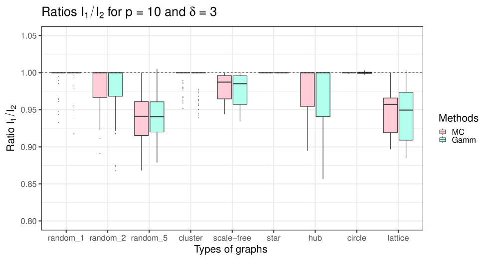
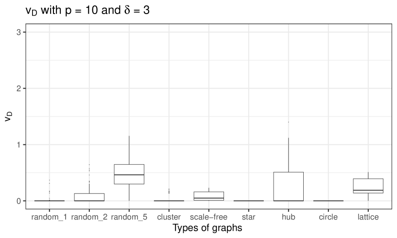
Figure 10: (Top) The boxplot for the ratio $I_{1}/I_{2}$ computed by the MC approach of Atay-Kayis and Massam (2005) (in red) and approximation (20) (in blue). (Bottom) The boxplot of the variance $v_{D}$ of $b_{1}$ for the corresponding graphs. These computations are done over 100 replications for nine different graphs (Figure 6) with $p=10$ nodes and $\delta=3$.

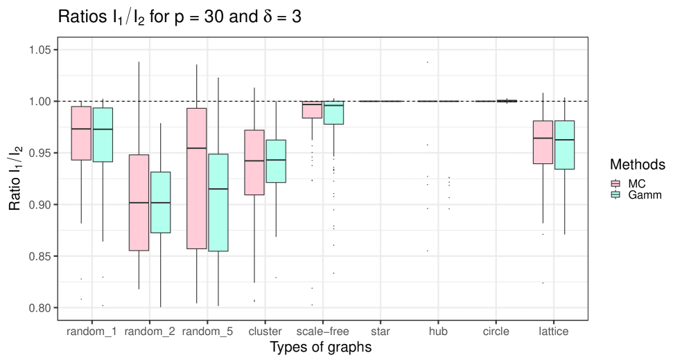
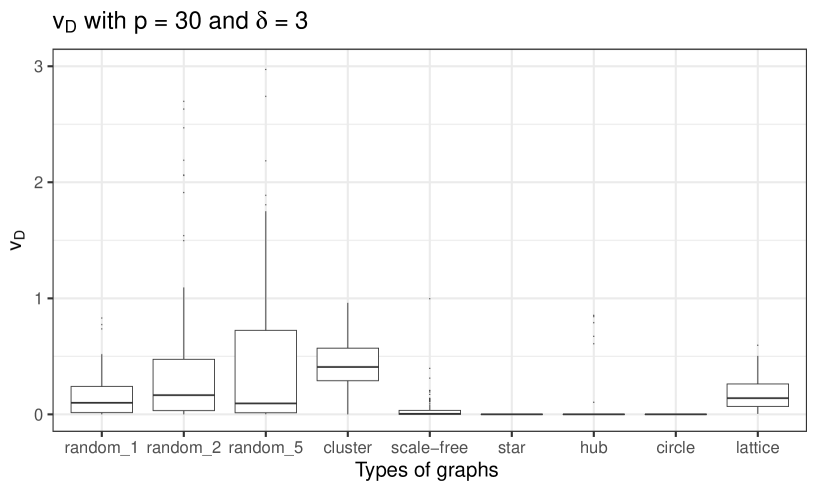
Figure 11: (Top) The boxplot for the ratio $I_{1}/I_{2}$ computed by the MC approach of Atay-Kayis and Massam (2005) (in red) and our approximation (20) (in blue). (Bottom) The boxplot of the variance $v_{D}$ of $b_{1}$ for the corresponding graphs. These computations are done over 100 replications for nine different graphs (Figure 6) with $p=30$ nodes and $\delta=3$.

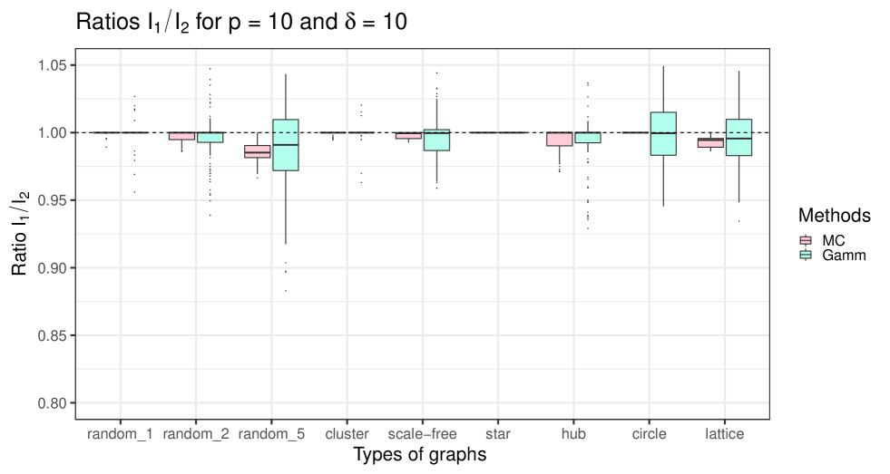
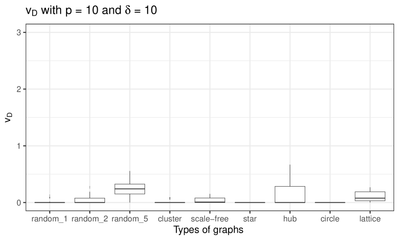
Figure 12: (Top) The boxplot for the ratio $I_{1}/I_{2}$ computed by the MC approach of Atay-Kayis and Massam (2005) (in red) and our approximation (20) (in blue). (Bottom) The boxplot of the variance $v_{D}$ of $b_{1}$ for the corresponding graphs. These computations are done over 100 replications for nine different graphs (Figure 6) with $p=10$ nodes and $\delta=10$.

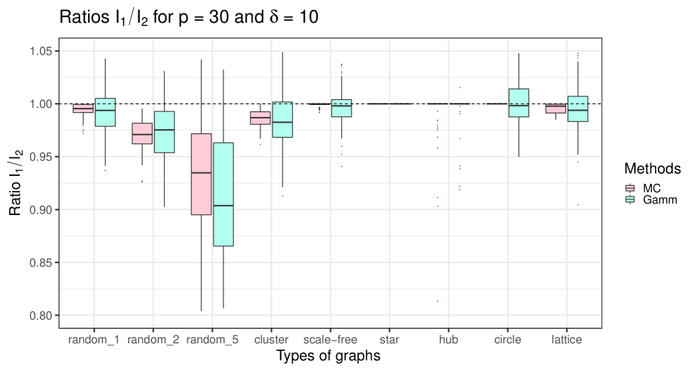
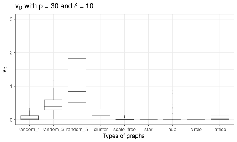
Figure 13: (Top) The boxplot for the ratio $I_{1}/I_{2}$ computed by the MC approach of Atay-Kayis and Massam (2005) (in red) and our approximation (20) (in blue). (Bottom) The boxplot of the variance $v_{D}$ of $b_{1}$ for the corresponding graphs. These computations are done over 100 replications for nine different graphs (Figure 6) with $p=30$ nodes and $\delta=10$.

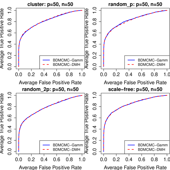
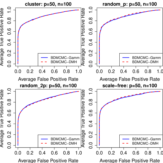
Figure 14: ROC curves for the BDMCMC algorithm with our approximation in Equation 8 (BDMCMC-Gamm) and BDMCMC algorithm with exchange algorithm (BDMCMC-DMH), over $50$ replications. Here, $p=50$, $n\in\{50,100\}$, and $4$ different graph structures.

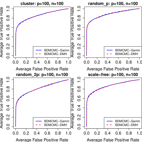
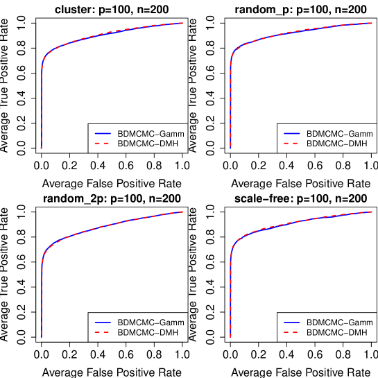
Figure 15: ROC curves for the BDMCMC algorithm with our approximation in Equation 8 (BDMCMC-Gamm) and BDMCMC algorithm with exchange algorithm (BDMCMC-DMH), over $50$ replications. Here, $p=100$, $n\in\{100,200\}$, and $4$ different graph structures.

References

- Abramovitz and Stegun (1972) Abramovitz, M. and I. Stegun (1972). Handbook of Mathematical Functions, Volume 55. National Bureau of Standards, Applied Mathematics.
- Albert and Barabási (2002) Albert, R. and A. Barabási (2002). Statistical mechanics of complex networks. Reviews of modern physics 74(1), 47.
- Atay-Kayis and Massam (2005) Atay-Kayis, A. and H. Massam (2005). A Monte Carlo method for computing the marginal likelihood in nondecomposable Gaussian graphical models. Biometrika 92(2), 317–335.
- Chamayou and Letac (1991) Chamayou, J.-F. and G. Letac (1991). Explicit stationary distributions for compositions of random functions and products of random matrices. Journal of Theoretical Probability 4(1), 3–36.
- Cheng and Lenkoski (2012) Cheng, Y. and A. Lenkoski (2012). Hierarchical Gaussian graphical models: Beyond reversible jump. Electronic Journal of Statistics 6, 2309–2331.
- Dempster (1972) Dempster, A. P. (1972). Covariance selection. Biometrics, 157–175.
- Dobra and Lenkoski (2011) Dobra, A. and A. Lenkoski (2011). Copula Gaussian graphical models and their application to modeling functional disability data. The Annals of Applied Statistics 5(2A), 969–993.
- Dobra et al. (2011) Dobra, A., A. Lenkoski, and A. Rodriguez (2011). Bayesian inference for general Gaussian graphical models with application to multivariate lattice data. Journal of the American Statistical Association 106(496), 1418–1433.
- Friedman et al. (2008) Friedman, J., T. Hastie, and R. Tibshirani (2008). Sparse inverse covariance estimation with the graphical lasso. Biostatistics 9(3), 432–441.
- Green (1995) Green, P. (1995). Reversible jump markov chain Monte carlo computation and Bayesian model determination. Biometrika 82(4), 711–732.
- Green (2003) Green, P. (2003). Trans-dimensional Markov chain Monte Carlo. Oxford Statistical Science Series, 179–198.
- Hinne et al. (2014) Hinne, M., A. Lenkoski, T. Heskes, and M. van Gerven (2014). Efficient sampling of gaussian graphical models using conditional bayes factors. Stat 3(1), 326–336.
- Hinoveanu et al. (2018) Hinoveanu, L. C., F. Leisen, and C. Villa (2018). A loss-based prior for gaussian graphical models. arXiv preprint arXiv:1812.05531.
- Lauritzen (1996) Lauritzen, S. (1996). Graphical Models, Volume 17. Oxford University Press, USA.
- Lenkoski (2013) Lenkoski, A. (2013). A direct sampler for G-Wishart variates. Stat 2(1), 119–128.
- Lenkoski and Dobra (2011) Lenkoski, A. and A. Dobra (2011). Computational aspects related to inference in Gaussian graphical models with the g-wishart prior. Journal of Computational and Graphical Statistics 20(1), 140–157.
- Letac and Massam (2020) Letac, G. and H. Massam (2020). Gaussian approximation of gaussian scale mixture. kybersetika 56(6), 1063–1080.
- Letac et al. (2007) Letac, G., H. Massam, et al. (2007). Wishart distributions for decomposable graphs. The Annals of Statistics 35(3), 1278–1323.
- Liang (2010) Liang, F. (2010). A double Metropolis–Hastings sampler for spatial models with intractable normalizing constants. Journal of Statistical Computation and Simulation 80(9), 1007–1022.
- Mohammadi and Wit (2015) Mohammadi, A. and E. Wit (2015). Bayesian structure learning in sparse Gaussian graphical models. Bayesian Analysis 10(1), 109–138.
- Mohammadi and Wit (2019a) Mohammadi, R. and E. Wit (2019a). BDgraph: Bayesian Structure Learning in Graphical Models using Birth-Death MCMC. R package version 2.62.
- Mohammadi and Wit (2019b) Mohammadi, R. and E. C. Wit (2019b). BDgraph: An R package for Bayesian structure learning in graphical models. Journal of Statistical Software 89(3), 1–30.
- Murray et al. (2006) Murray, I., Z. Ghahramani, and D. MacKay (2006). MCMC for doubly-intractable distributions. Proceedings of the 22nd Annual Conference on Uncertainty in Artificial Intelligence, 359–366.
- Park and Haran (2018) Park, J. and M. Haran (2018). Bayesian inference in the presence of intractable normalizing functions. Journal of the American Statistical Association 113(523), 1372–1390.
- Roverato (2002) Roverato, A. (2002). Hyper inverse Wishart distribution for non-decomposable graphs and its application to Bayesian inference for Gaussian graphical models. Scandinavian Journal of Statistics 29(3), 391–411.
- Rue and Held (2005) Rue, H. and L. Held (2005). Gaussian Markov random fields: theory and applications. CRC press.
- Uhler et al. (2018) Uhler, C., A. Lenkoski, and D. Richards (2018). Exact formulas for the normalizing constants of Wishart distributions for graphical models. The Annals of Statistics 46, 90–118.
- Wang (2012) Wang, H. (2012). The Bayesian graphical Lasso and efficient posterior computation. Bayesian Analysis 7, 771–790.
- Wang and Li (2012) Wang, H. and S. Li (2012). Efficient Gaussian graphical model determination under G-Wishart prior distributions. Electronic Journal of Statistics 6, 168–198.