Jammed spin liquid in the bond-disordered kagome Heisenberg antiferromagnet

Abstract

We study a class of continuous spin models with bond disorder including the kagome Heisenberg antiferromagnet. For weak disorder strength, we find discrete ground states whose number grows exponentially with system size. These states do not exhibit zero-energy excitations characteristic of highly frustrated magnets but instead are local minima of the energy landscape. This represents a spin liquid version of the phenomenon of jamming familiar from granular media and structural glasses. Correlations of this jammed spin liquid, which upon increasing the disorder strength gives way to a conventional spin glass, may be algebraic (Coulomb-type) or exponential.

Introduction: A large ground state degeneracy is a defining feature of strong geometric frustration in classical spin systems. It underpins much of their exotic properties, in particular the emergence of topological spin liquids Moessner and Ramirez (2006). For discrete spins Wannier (1950); Anderson (1956), the number of ground states can scale exponentially in the system size, whereas for continuous spins the ground states form a manifold whose dimension is proportional to the system size. Comparatively little is known about the effect of disorder and lattice distortions, with some pioneering works having unearthed both a capacity of spin liquids to accommodate disorder Shender et al. (1993); Moessner and Berlinsky (1999); Henley (2001), and an immediate instability towards spin glassiness for arbitrarily weak disorder Bellier-Castella et al. (2001); Saunders and Chalker (2007); Andreanov et al. (2010); Savary et al. (2011); Wang et al. (2007); Chern et al. (2008); Roychowdhury et al. (2017). Given their large degeneracy, the geometrically frustrated magnets should be particularly susceptible to perturbations and disorder in the ideal structure. Such perturbations are necessarily present in real materials and may themselves induce new phenomena Cépas and Canals (2012); Sala et al. (2014); Sen and Moessner (2015); Savary and Balents (2017). In addition, it has recently been realized that the field of classical spin liquids may be richer than appreciated so far. New arrivals include an anisotropic pyrochlore magnet exhibiting pinch-lines in the excitation spectrumBenton et al. (2016), as well as spin liquids exhibiting exponential, rather than Coulomb, correlations in the limit of low temperatures Rehn et al. (2017).

Here, we present a family of continuous spin models which exhibit a novel jammed spin liquid regime with an exponentially large set of discrete ground states. We study in depth the kagome Heisenberg magnet, where the jammed spin liquid appears most naturally. Like in the clean system, the ground-state spin configurations minimize energy for every triangle, but in contrast to it, they remain disconnected exhibiting no non-trivial zero-energy modes. Still they show a softer spectrum than that of a spin glass, which in turn appears at higher disorder strength. Depending on model details, the jammed spin liquid either inherits the algebraic Coulomb correlations, or exhibits a disorder-screened version thereof.

Transitions in constraint satisfiability in continuous systems, at which an exponential number of discrete ground states appear, are known in the context of structural glasses and granular media under the heading of jamming Liu and Nagel (1998); O’Hern et al. (2003); Liu and Nagel (2010), from which we have borrowed the term. Our model is a natural extension of these ideas to frustrated spin systems, and we discuss possible interactions between these fields in the outlook.

Our analysis utilizes a number of different methods, including direct numerical searches for ground states, and combining these with analytical continuity arguments. In addition, we perform calculations within the self-consistent Gaussian approximation (SCGA) Garanin (1996) to study the correlations on large systems, as well as Monte-Carlo (MC) simulations to access finite temperature properties and the spin glass phase. We finish with an outlook and a discussion of connections to physics beyond spin systems.

Model Hamiltonian: Our starting point is the classical Heisenberg model of $O(3)$ spins on a kagome lattice

$$H = \sum_{\langle ij\rangle}J_{ij}\,{\bf{S}}_{i}\cdot{\bf{S}}_{j}\ ,$$ (1)

with random nearest-neighbor exchanges $J_{ij}>0$. For every triangle $\alpha$ formed by sites $ijk$, see Fig. 1(a), we define $\gamma_{i\alpha}=\sqrt{{J_{ij}J_{ik}}/{J_{jk}}}$ and rewrite $H$ as

$$H=\frac{1}{2}\sum_{\alpha}{\bf{L}}_{\alpha}^{2},\quad\text{with}\quad{\bf{L}}_{\alpha}=\sum_{i\in\alpha}\gamma_{i\alpha}{\bf{S}}_{i}\,,$$ (2)

up to a constant energy shift. The above form provides a set of local ground-state constraints, which may or may not be satisfied simultaneously, see below. Inversely, Eq. (2) generates a bond-disordered model (1) with couplings $J_{ij}=\gamma_{i\alpha}\gamma_{j\alpha}$ between spins $ij$ in triangle $\alpha$.

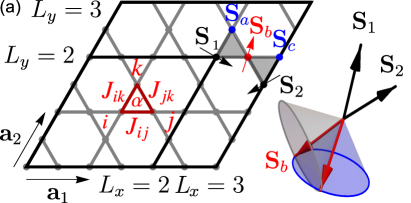
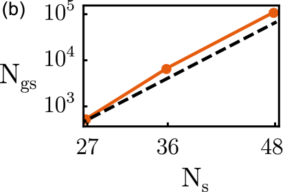
Figure 1: (a) Illustration of finite-size kagome lattices with primitive lattice vectors $\mathbf{a}_{1}=(1,0)$ and $\mathbf{a}_{2}=(1,\sqrt{3})/2$. Spins in triangle $\alpha$ at sites $i,j,k$ are coupled via $J_{ij}$. Black parallelograms demark the edges of square $L=L_{x}=L_{y}=2,3$ systems, for periodic boundary conditions opposite edges are identified. Marked spins/triangles pertaining to the transfer matrix construction (see text). (b) Number of ground states $N_{gs}$ vs. number of spins $N_{\mathrm{s}}$ compared with the scaling $N_{\mathrm{gs}}\sim 2^{N_{\mathrm{s}}/3}$ (dashed line).

More generally, the Hamiltonian (2) can be defined for $O(n)$ spins on frustrated lattices consisting of fully-connected units/simplices of $q$ spins: $n=2,3$ for $XY$ and Heisenberg spins, whereas $q=3,4$ for triangles and tetrahedra. For $\gamma_{i\alpha}\equiv 1$, one recovers the regular frustrated spin models for a range of lattices, such as kagome, checkerboard, pyrochlore or maximally frustrated honeycomb models, all of which exhibit order by disorder (obdo) for small $n$ Chalker et al. (1992); Ritchey et al. (1993); Harris et al. (1992); Moessner and Chalker (1998a); *MoessnerPyro1998; Rehn et al. (2016) and a classical spin liquid for large $n$ Garanin and Canals (1999); Moessner and Chalker (1998a); *MoessnerPyro1998. For $q>3$, a bond-disordered model (1) generated by (2) has correlations between bond amplitudes in the same simplex. For the kagome lattice ($q=3$) the mapping between $J_{ij}$ and $\gamma_{i\alpha}$ is one-to-one, and therefore we focus on this example as the most natural one (for the $XY$ spins on the checkerboard lattice see sup ).

We identify and study two classes of distributions of $J_{ij}$ on the kagome lattice with somewhat different phenomenology. The first one is the bond-disorder model (BDM) with $J_{ij}$ chosen uniformly within $(1-\delta,1+\delta)$ and $\delta<1$. The second class called the ‘maximally disordered Coulomb model’ (MCM) is constructed from Eq. (2) in the following way: we set $\gamma_{i\alpha}=\gamma_{i}\gamma_{\alpha}$ assigning a factor $\gamma_{i}$ to every spin and an additional factor $\gamma_{\alpha}$ to every triangle. Both are chosen uniformly within $(1-\delta,1+\delta)$ which ensures that the models have the same critical point $\delta_{c}$ sup ). The MCM is defined by $5L^{2}$ random parameters as opposed to $6L^{2}$ for the BDM. We believe that MCM is the most general model preserving the Coulomb correlations; in particular, it saturates the number of degrees of freedom allowed accounting for $L^{2}$ “star-conditions” very recently identified in Ref. Roychowdhury et al. (2017).

Ground state construction and counting: The lowest-energy classical spin configurations must satisfy the set of local constraints

$${\bf{L}}_{\alpha}=0\ \ \ \forall\alpha\ .$$ (3)

For an isolated triangle $\alpha$, the constraint implies that three vectors $\gamma_{i\alpha}{\bf S}_{i}$ form a closed triangle in spin space with side lengths $\gamma_{i\alpha}$. This can be always achieved once the corresponding $\gamma_{i\alpha}$ obey the triangle inequality, which in turn restricts $\delta\leq 1/3$ sup . For the full lattice, an indicator of the dimensionality of the ground state manifold is given by the Maxwellian counting argument which compares the number of the degrees of freedom $D$ to the number of ground state constraints $K$. Similar to the regular kagome Heisenberg antiferromagnet Moessner and Chalker (1998a), $D=K$ in our case suggesting no degeneracy. However, the constraint counting does not account for possibly dependent or inconsistent constraints. Next, we give an explicit construction, which shows that ground states of the full system are generically discrete and provides an estimate of their number.

To construct the ground states in the bulk, i.e., ignoring the boundaries, we proceed from layer to layer in the spirit of a transfer matrix. Let us consider the group of three spins $\mathbf{S}_{a}$, $\mathbf{S}_{b}$, $\mathbf{S}_{c}$, see Fig. 1, such that all spins in the lower layer and to the left of the group are already fixed. The three spins belong to a pair of up/down triangles of the lattice. In each of the two triangles one spin $\mathbf{S}_{1(2)}$ is fixed and one unknown spin $\mathbf{S}_{b}$ (red) is shared between the up and down triangles. The ground state constraint determines angles between spins in a triangle, the only remaining freedom is rotation of the undetermined spins around the fixed spin $\mathbf{S}_{1(2)}$. This rotation makes the common spin $\mathbf{S}_{b}$ sweep out two distinct conic sections (whose opening angle depends on the random bond couplings) of the unit sphere as shown in Fig. 1, which generically have either none or two points of intersection. When there are two intersection points, there is a discrete choice between them, yielding an orientation of $\mathbf{S}_{b}$ consistent with the constraints in both triangles. This step is then repeated to determine all spins throughout the lattice.

Ignoring the possibility of inconsistent constraints that yield no crossing, the above procedure estimates the number of ground states as $N_{\mathrm{gs}}\sim 2^{N_{s}/3}$ for $N_{s}$ spins in the lattice in accordance with the number of up-down triangle pairs. Interestingly, the corresponding entropy ${\cal S}/N_{s}\approx\frac{1}{3}\ln 2$ is larger than the entropy of the well-known coplanar states of the clean system ${\cal S}/N_{s}\approx\ln(1.13)$ Baxter (1970). Figure 1(b) shows enumeration results on small finite systems consistent with the derived scaling. We also provide arguments for the continuity of each state as a function of $\delta$ in the Supplemental Material sup .

Correlations:

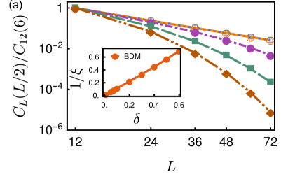
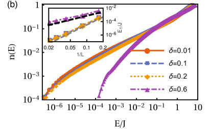
Figure 2: (a) Finite-size scaling of $C_{L}(L/2)=\langle\mathbf{S}(0)\cdot\mathbf{S}(L/2)\rangle$ on a log-scale for MCM (open symbols) and BDM (filled symbols) for $\delta=0.1,0.2,0.3$ (circles, squares, diamonds) on $L\times L$ systems. Inset: Inverse of the correlation length $1/\xi$ as a function of $\delta$ obtained from the long distance behaviour, $\langle\mathbf{S}(0)\cdot\mathbf{S}(r)\rangle\sim e^{-r/\xi}$, of the BDM on a $144\times 36$ system. (b) Cumulative density of the eigenvalues of the Hessian matrix for the jammed spin liquid $\delta<1/3$ and spin glass. Inset: Scaling of the lowest (non-trivial) eigenvalue $E_{1}$ shows the relative softness of the jammed spin liquid. Dashed lines are guides to the eye with $L^{-2}$ (black) and $L^{-4}$ (gray).

We compute the correlations within the SCGA which is exact in the limit of spin components $n\rightarrow\infty$ Stanley (1968), and provides quantitative results for the low temperature correlations at finite $n$ Garanin and Canals (1999). It allows to access considerably larger systems than with explicit energy minimisation; where both are possible, the results agree with each other and with our Monte Carlo simulations sup .

There is a fundamental difference between BDM and MCM, as displayed in Fig. 2(a), which shows the finite-size scaling analysis of $C_{L}(L/2)=\langle\mathbf{S}(0)\cdot\mathbf{S}(L/2)\rangle$. The MCM retains the algebraic correlations characteristic of the Coulomb phase present at large-$n$, but does not exhibit the peaks present for the disorder-free case of $n=3$ resulting from order by disorder. By contrast, the BDM finds a crossover to exponential decay with a correlation length $\xi\sim 1/\delta$ (inset of Fig. 2(a)). This follows from the fact that the MCM straightforwardly permits the definition of a height-model (which implies the $L^{-2}$ behaviour) analogous to the disorder-free case Huse and Rutenberg (1992), whereas in the BDM this appears to be impossible. The screened correlations of the BDM are comparable to those of the clean system at a temperature $T^{*}\sim\delta^{2}$ (suppl. mat. sup ).

Low energy spectrum of Hessian: We study the quadratic energy cost of deformations of the ground states via the spectrum of the Hessian matrix. Importantly, we find no zero-modes for either the BDM or the MCM. This is in stark contrast to the coplanar states of the clean kagome system which have an extensive number of exact zero-modes. In the language of mechanical lattices our spin ground states are fully rigid Kane and Lubensky (2014); Lawler (2016).

Nonetheless, we find that the excitations in the jammed spin-liquid are considerably softer than in a spin glass, see Fig. 2(b), e.g. in that the smallest eigenvalue of the Hessian spectrum vanishes with a higher power of system size. We also note that at small $\delta$, the spectrum appears to become independent of $\delta$, suggesting it also describes the excitations of the discrete noncoplanar ground states of the disorder-free system.

Phase Diagram (Fig. 3):

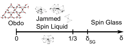
Figure 3: Phase Diagram as a function of disorder strength, with the jammed spin liquid appearing for $0<\delta<1/3$. Illustrations are of the $\sqrt{3}\times\sqrt{3}$ state and of non-coplanar finite size jammed spin-liquid states. The precise value of $\delta_{\mathrm{SG}}\geq\delta_{c}$ is not known.

The jammed spin liquid is terminated by two different states for low and high $\delta$. We consider these in turn.

The clean system, $\delta=0$, is the archetypal frustrated magnet exhibiting order by disorder in the form of coplanar states Chalker et al. (1992); Ritchey et al. (1993); Harris et al. (1992); Huse and Rutenberg (1992); Zhitomirsky (2008) with weak $\sqrt{3}\times\sqrt{3}$ translational symmetry breaking Zhitomirsky (2008); Chern and Moessner (2013). Bond disorder is inconsistent with coplanarity in the sense that the energy of coplanar states exceeds that of the non-coplanar ground states (suppl. mat. sup ). Since the order by disorder is driven by excess soft modes, it can be diagnosed by their signature in the reduced heat capacity Chalker et al. (1992). The heat capacity, computed from fluctuations of the internal energy in the MC simulations as $C=\left(\langle E^{2}\rangle-\langle E\rangle^{2}\right)/T^{2}$, is shown in the inset of Fig. 5. The disorder-free value of $C=11/12$ at low temperatures Chalker et al. (1992); Zhitomirsky (2008) is replaced by $C=1$ for any $\delta>0$ consistent with our finding that there is no extensive number of soft modes. In addition, we clearly observe three distinct signatures in the heat capacity, a “dip” in the JSL phase ($\delta=0.1$), an intermediate regime with flat behaviour ($\delta=0.4$), and a ”bump“ in the spin glass phase ($\delta=0.6$).

Throughout the jammed spin liquid, the ground state constraints are obeyed, exactly for the MCM (suppl. mat sup ); for the BDM, there is one unsatisfiable global constraint imposed by the periodic boundary conditions. The total sum of spins on the up and down triangles has to be equal, as this just amounts to a different bookkeeping of all the spins in the system. Indeed, we find that (Fig. 4) for $\delta<\delta_{c}$, $\left<\mathbf{L}_{\Delta}^{2}\right>\sim L^{-4}$ vanishes in the thermodynamic limit, consistent with a single (or more generally a non-extensive number of) unsatisfiable constraints distributed over $N_{\Delta}\sim L^{2}$ triangles.

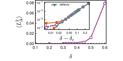
Figure 4: Residual energy per triangle of the BDM vs. $\delta$ for $L=12,24,36,48$ (circles, triangles, diamonds, squares). Inset: Same on a log-scale vs. $\delta-\delta_{c}$ consistent with $\left<\mathbf{L}_{\Delta}^{2}\right>\sim(\delta-\delta_{c})^{5}$and from a direct evaluation of the energy of “defect” triangles with collinear spins.

The jammed spin liquid regime terminates at a critical disorder strength $\delta_{c}=1/3$. This threshold is related to the impossibility to satisfy the local constraint ${\bf{L}}_{\alpha}=0$ for a large disparity between bond values. Beyond $\delta_{c}$ coupling configurations appear for which the groundstate constraint cannot be satisfied (suppl.mat. sup ). Near $\delta_{c}=1/3$, the probability of choosing such bond couplings $\{J_{ij}\}$ grows as $(\delta-\delta_{c})^{3}$. Together with ${\bf{L}}_{\Delta}\sim(\delta-\delta_{c})$ this yields $\left<\mathbf{L}_{\Delta}^{2}\right>\sim\delta^{5}$, in agreement with an analysis of a single triangle, $\left<\mathbf{L}_{\Delta}^{2}\right>\sim\frac{27}{5}\left[\frac{3}{2}\left(\delta-\delta_{c}\right)\right]^{5}$.

On further increasing $\delta$, the system turns into a conventional spin glass beyond a $\delta_{\mathrm{SG}}\geq\delta_{c}$ as evidenced by the diverging spin-glass susceptibility (Fig. 5). In the jammed spin-liquid $\delta<\delta_{c}$ and for intermediate $\delta_{C}<\delta<\delta_{\mathrm{SG}}$, $\chi_{\mathrm{SG}}(T)$ remains flat down to the lowest temperatures.

Open questions and connections: A number of questions follow naturally from this study, e.g. whether the jammed spin liquid entropy may be determined exactly. Also, its low-temperature dynamical properties should be worth investigating, as it appears to fit neither previous examples of conventional spin liquids or kagome Heisenberg magnets Moessner and Chalker (1998a); *MoessnerPyro1998; Conlon and Chalker (2009); Robert et al. (2008); Taillefumier et al. (2014); Keren (1995), nor a Halperin-Saslow picture of a disordered magnet with a finite spin stiffness Halperin and Saslow (1977).

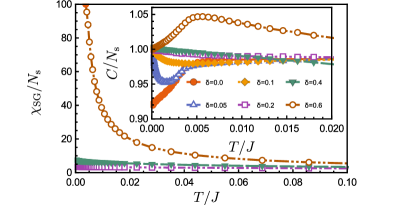
Figure 5: Spin glass susceptibility $\chi_{\mathrm{SG}}$ vs. temperature in units of the bond strength $T/J$ from MC simulations for the BDM. Inset: Specific heat per spin $C/N_{\mathrm{s}}$ vs. temperature showing absence of order by disoder for $\delta>0$.

Regarding the phase diagram, we have not numerically determined the exact point, $\delta_{SG}\geq\delta_{c}$ of the spin glass transition. The possibility of another new regime for $\delta_{c}<\delta<\delta_{SG}$ appears not unnatural given, (i) that the excess energy for $\delta>\delta_{c}$ can be captured by just counting the number of triangles with collinear spins, without taking into account any collective physics between them, (ii) neither $C$ (Fig 5) nor $\chi_{\mathrm{SG}}$ (suppl. mat. sup ) show within our numerical precision indications of non-analytical behaviour even at $\delta=0.4$, (iii) the capacity of spin liquids to screen disorder Rehn et al. (2015).

Potential candidate materials are the kagome hydronium jarosites Wills and Harrison (1996); Bisson and Wills (2008), which even though showing a spin freezing transition Wills et al. (2000a), appear to be different from conventional spin glasses Wills et al. (2000b); Dupuis et al. (2002); Ladieu et al. (2004). Besides disorder and geometric frustration, the anisotropic distortion may cause glassy behavior in these systems Bisson and Wills (2008), and it is an interesting question whether anisotropy or second-neighbor interactions would stabilize the glassy phase in the model studied here. In contrast to the pyrochlore lattice where infinitesimal disorder produces a spin-glass transition Saunders and Chalker (2007), we find the spin liquid to be stable for the kagome-lattice model. This implies that for antiferromagnetic materials with the kagome structure, weak disorder alone cannot account for the observed spin freezing.

The termination of the jammed spin liquid is of broader interest on account of its connection to other fields of statistical mechanics. The marginality of the kagome Heisenberg magnet in Maxwellian constraint counting was noted already a long time back Moessner and Chalker (1998a); *MoessnerPyro1998, when it was also realized that such marginal constraint tends to underpin the order by disorder phenomenon, which we have here found is in turn suppressed by bond disorder. Recent developments have emphasized connections to a broader class of systems, in particular mechanical Maxwell lattices Kane and Lubensky (2014), with implications for topological aspects of the excitation spectrum, and the local stability of distorted kagome ground states Lawler (2016); Roychowdhury et al. (2017), which may be of relevance to our numerics on the Hessian matrix.

Investigating the connection of our spin model to ‘conventional’ jamming Liu and Nagel (1998); O’Hern et al. (2003); Liu and Nagel (2010), will be a most interesting topic for future study. Dynamical and nonlinear properties should be of particular interest, see e.g. the very recent preprints Lubchenko and Wolynes ; Wu et al. . Crucially, there are some properties specific to our setting, including an extended and stable jammed regime; the gradual onset and spatial localization of the added constraints; the possibility of the satisfiable regions of the system acting as a medium generating effective interactions between the latter; and the peculiar onset of the nonzero energy density, which in turn will depend on details of the disorder distribution.

This set of questions has also been given concerted attention in a more ”computer-science” context Franz et al. (2017), where the low (high)-disorder regime corresponds to the (UN)SAT regime of a constraint-satisfaction problem. [In passing, we note that in the language of that community, the SAT/jammed spin liquid regime is unfrustrated, as all terms in the Hamiltonian can be simultaneously satisfied.] We hope our work will stimulate work establishing connections between all of these topics.

Acknowledgements: We thank J. T. Chalker, Chris Laumann, A. Scardicchio for helpful discussions, and V. Vitelli for pointing us in the direction of the jamming phenomena. This work was in part supported by Deutsche Forschungsgemeinschaft via SFB 1143.

Supplemental Material: Jammed spin liquid in the bond-disordered kagome Heisenberg antiferromagnet

I Kagome model

Analysis of a single triangle: For both the BDM and the MCM models the critical disorder strength $\delta_{c}$ is related to the impossibility to satisfy the local constraint $L_{\alpha}=\sum_{i\alpha}\gamma_{i\alpha}\mathbf{S}_{i}=0$. Geometrically, this means that the spins form a closed triangle with side lengths $\gamma_{i\alpha}$. Thus, there is no possible solution if any side is larger than the sum of the other two $\gamma_{1}>\gamma_{2}+\gamma_{3}$. We also note that this shows that the minimal energy in an isolated triangle is $0$ if $\gamma_{1}\leq\gamma_{2}+\gamma_{3}$ and $\gamma_{1}-(\gamma_{2}+\gamma_{3})$ if $\gamma_{1}>\gamma_{2}+\gamma_{3}$ (where we assume them to be ordered in decreasing magnitude). The critical point occurs exactly when side lengths that satisfy $\gamma_{1}=\gamma_{2}+\gamma_{3}$ become possible, the triangle in spin space becomes a collinear configuration with two parallel spins with small side lengths anti-parallel to a third spin with a large side length. Below we will refer to triangles that do not allow a zero-energy solution as “defect” triangles.

We illustrate this transition in Fig. S1 for increasing disparity between two small and one large side length as relevant to the transitions in the BDM and MCM.

Figure S1: The groundstate constraint $\gamma_{1}\mathbf{S}_{1}+\gamma_{2}\mathbf{S}_{2}+\gamma_{3}\mathbf{S}_{3}=0$ implies that the spins form a closed triangle. Here illustrated for $\gamma_{1}=1+\delta$, $\gamma_{2}=\gamma_{3}=1-\delta$ with $\delta=0.1,0.3,0.333$.

We show below that for the choices of the couplings made in the main text, both models have the same critical point $\delta_{c}=1/3$.

For the MCM we have $\gamma_{i\alpha}=\gamma_{i}\gamma_{\alpha}$. For the groundstate constraint $\gamma_{\alpha}$ does not matter as it is a common factor for all spins in a triangle. As we choose $\gamma_{i}$ in $(1-\delta,1+\delta)$ we have at the critical point

$$(1+\delta_{c}) =2\,(1-\delta_{c})\,,$$ (S1)

thus $\delta_{c}^{\textrm{MCM}}=1/3$.

For the BDM we have $\gamma_{i\alpha}=\sqrt{\frac{J_{ij}J_{ik}}{J_{jk}}}$ and $J_{ij}$ in $(1-\delta,1+\delta)$. To obtain two minimal scaling factors and one maximal scaling factor the couplings need to be $J_{ij}=1-\delta$ and $J_{jk}=J_{ik}=1+\delta$. Then we have at the critical point

$$\sqrt{\frac{(1+\delta_{c}^{\textrm{BDM}})(1+\delta_{c}^{\textrm{BDM}})}{1-\delta_{c}^{\textrm{BDM}}}} =2\,\sqrt{\frac{(1+\delta_{c})(1-\delta_{c})}{1+\delta_{c}}}\,,$$ (S2)

thus, $\delta_{c}^{\textrm{BDM}}=1/3$.

We emphasise that this reasoning is based on the study of a single isolated triangle. The fact that the model on the full connected kagome lattice shows the transition at the same point is non-trivial.

Counting ground states: We numerically search for ground states of the MCM with a fixed disorder realisation at disorder strength $\delta=0.1$. We perform this search on periodic clusters of linear dimensions $(L_{x},L_{y})=(2,2),(3,3),(4,3),(4,4)$ obtaining $10^{3},10^{4},10^{5},10^{6}$ ground states.

For each of these states we compute the spectrum of its Hessian. We then classify the ground states into distinct groups according to the first 10 eigenvalues of the spectrum. In table 1 we summarise the results of these enumeration searches.

$L_{x},L_{y}$	Samples	$2^{N_{\mathrm{s}}/3}$	$N_{\mathrm{gs}}$
2,2	$10^{3}$	16	4
3,3	$10^{4}$	512	558
4,3	$10^{5}$	4096	6910
4,4	$10^{6}$	65536	113899

Table 1: Results of the enumeration search. System sizes, Number of ground state searches, $2^{N_{\mathrm{s}}/3}$expected number of ground states based on the bulk scaling, $N_{\mathrm{gs}}$ number of distinct ground states found.

Characteristic distributions of the frequency counts, i.e. the probabilities that a ground state occurs a certain number of times in our search are shown in Fig. S2, which permit an estimate of the number of ground states missed by the search by fitting to a Poissonian distribution.

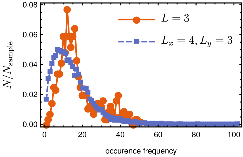
Figure S2: Number of ground states $N$ that occur with given frequency in our ground state search normalised to total number of samples.

State continuity and fidelity: Here, we consider the evolution of the classical ground states with disorder strength and their connection to the states of the clean model via the state fidelity.

To this end we fix a particular disorder realisation $J_{ij}=1+\delta_{ij}$ with $\delta_{ij}$ uniform in $(-1,1)$ and then rescale the random part $\delta_{ij}$ by the disorder strength $\delta$. We then define the fidelity $F$ between states for a fixed disorder realisation at different disorder strengths as $F(\delta,h)=\left|\langle S(\delta-h)|S(\delta+h)\rangle\right|=\prod_{i=1}^{N_{\mathrm{s}}}\left|\mathbf{S}_{i}(\delta-h)\cdot\mathbf{S}_{i}(\delta+h)\right|$, where we use $|S(\delta)\rangle$ as a shorthand for the full spin configuration $\{\mathbf{S}_{i}(\delta)\}$ at a disorder strength $\delta$, the scalar product between spins $\mathbf{S}_{i}$ is the usual vector scalar product and we rotate the spin configurations $\{\mathbf{S}_{i}\}$ such that $\mathbf{S}_{1}$ coincides between both. Defined in this way we expect the fidelity to change quadratically in $h$ for small $h$ and be exponential in the number of spins $N_{s}$.

The state fidelity is well established as a diagnostic for phase transitions in quantum systems [1, 2]. However, for classical systems the choice of the scalar product is somewhat arbitrary. We emphasise that here we mainly use it in the basic analysis sense, where we view the classical ground states as functions of a parameter $\delta$ and simply ask for continuity or differentiability of this function.

In Fig. S3 we show the disorder average of the logarithmic fidelity normalised to the number of sites $\langle\log F(\delta,h)/(N_{\mathrm{s}}h^{2})\rangle$ as a function of disorder strength. The fidelity clearly tracks the phase-transition at $\delta_{c}=1/3$ where the classical state changes rapidly for small changes of the system parameters. In addition, we observe a small peak in the low delta regime, which however scales to 0 for larger system sizes, whereas the peak at the transition scales with $N_{\mathrm{s}}$.

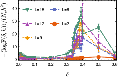
Figure S3: Logarithmic fidelity per site $\log F(\delta,h)/N_{s}$ for $h=0.001\delta$ of the groundstate at $T=0$.

This suggests that the states connect smoothly to the ground states of the clean kagome system in the limit $\delta\rightarrow 0$ and evolve smoothly up to the critical point at $\delta_{c}$. In the next section we provide semi-analytic arguments that support this picture.

Continuity of states and implicit function theorem: We may understand the evolution of the classical ground states of the model with disorder strength $\delta$ via the mapping

$$\begin{split}G:\quad&\mathbb{R}\times\mathbb{R}^{3N_{\mathrm{s}}}\rightarrow\mathbb{R}^{3N_{\mathrm{s}}}\\ &\delta\times\{\mathbf{S}_{i}\}\mapsto\begin{cases}\mathbf{S}^{2}_{i}-1&i\in 1,\dots,N_{S}\\ {\bf{L}}_{\alpha}&\alpha\in 1,\dots,2N_{\mathrm{s}}/3\end{cases}\end{split}$$ (S3)

where the dependence of ${\bf{L}}$ on the spins and $\delta$ is implicit. The ground state configurations then correspond to the preimage of the zero-vector, e.g. $\{\mathbf{S}^{\mathrm{gs}}_{i}\}=G^{-1}(\mathbf{0})$.

Given a ground state at some fixed disorder strength, e.g. a point $\{\delta_{0},\{\mathbf{S}_{i}\}\}$ such that $G(\{\delta_{0},\{\mathbf{S}_{i}\}\})=\mathbf{0}$, the implicit function theorem guarantees that the ground state is given by a differentiable function of the disorder strength $\delta$ in an open neighbourhood of $\delta_{o}$ if the Jacobian $\left[\frac{\partial G_{i}}{\partial S_{jd}}\right]$ is invertible. Here $j=1,\dots,N_{\mathrm{s}}$ is the site index and $d=x,y,z$ is the index of the spatial dimension.

Strictly speaking one needs to consider this mapping on the quotient space $\mathbb{R}^{3N_{\mathrm{s}}}/\mathrm{O}(3)$ to remove the (trivial) degeneracy due to global $\mathrm{O}(3)$ rotations. This can be done in different ways, e.g. by fixing one spin and one plane and considering the remaining coordinates. We find it more convenient simply to suppress the three zero singular values of the Jacobian corresponding to this degeneracy.

The implicit function theorem ensures both existence and the smooth dependence on disorder strength of the ground states, at least in some neighbourhood of a non-singular point. In particular, if all ground states are non-singular the number of ground states is also preserved when increasing the disorder strength. Further, when during this mapping one does not encounter a singular point, one can map all states back to ground states of the clean model at $\delta=0$, or starting from these obtain all ground states at finite disorder.

Based on the form of $G$ in Eq. S3 and its Jacobian one can already make some important observations: Firstly, for coplanar states the Jacobian is necessarily singular, thus, we do not expect coplanar states to connect to finite disorder ground states. Secondly, the Jacobian is also singular if two spins in a triangle are collinear. Consequently, as soon as defect triangles appear at $\delta_{c}$, the mapping based on the implicit function theorem breaks down.

To test whether the ground states we find actually are non-singular, we consider the lowest singular value of the Jacobian (suppressing the 3 zeros due to global rotation) for ground states found at different disorder configurations and strengths. In Fig.  S4 we show the lowest such value found over 1000 disorder realisations and 20 states for every point.

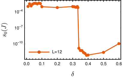
Figure S4: Lowest singular value $s_{0}$ (suppresing the three zeros due to global rotations) of the Jacobian of $G$, Eq. S3, found over different ground states ($T=0$) and disorder realisations at a strength $\delta$. This indicates whether the ground state may be continued locally via the inverse function theorem as $\delta<\delta_{c}$ is varied.

We clearly observe the transition at $\delta_{c}=1/3$ as explained by the appearance of defect triangles. Further, we find no singular states below the transition. Thus, we expect all ground states of the disordered system to connect smoothly to non-coplanar ground states of the clean system.

Fate of coplanarity: We consider the stability of coplanar states to disorder and establish that they are not part of the ground state manifold of the disordered models.

To do so we compare the minimal energy of spin configurations of 2 and 3 component spins respectively obtained by numerical optimisation and averaged over disorder realisations. The results for different disorder strengths and linear system sizes are shown in Fig. S5.

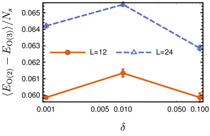
Figure S5: Energy difference per spin of ground states ($T=0$) of n-component spins $E_{\mathrm{O}(n)}$ for $n=3$ (Heisenberg) and $n=2$ (XY) as a function of disorder strength $\delta$ for linear system sizes $L=12,24$ with total number of spins $N_{\mathrm{s}}=3L^{2}$ averaged over disorder realisations.

We observe that the coplanar $\mathrm{O}(2)$ ground states always have a higher energy than the corresponding $\mathrm{O}(3)$ state. We emphasise that this is in fact true individually for all disorder realisations and not only for the mean. Moreover, this energy difference increases with increasing system size, and consequently would appear to remain finite in the thermodynamic limit.

We conclude that as the coplanar states have higher energy than the non-coplanar states entropic selection of coplanar states should not occur for the disordered model in contrast to the clean kagome antiferromagnet. This is consistent with our results on the heat capacity in the main text.

Residual energy of the MCM: In this section we provide the residual energy of the MCM as a function of disorder strength $\delta$ (the corresponding plot for the BDM can be found in the main text). In Fig. S6 we clearly observe the sharp transition at $\delta_{c}=1/3$ below which the residual energy per triangle $\langle\mathbf{L}^{2}_{\Delta}\rangle$ is strictly zero (within machine precision). In the inset we show a zoom into the behaviour close to the critical point. We observe the same scaling $\langle\mathbf{L}^{2}_{\Delta}\rangle\sim(\delta-\delta_{c})^{5}$ as for the BDM.

In addition, we again compare the residual energies obtained from the direct numerical optimisation with the prediction of “defects”. This estimate is obtained by individually minimising the energy independently on all triangles. As explained above for a single triangle, the minimal energy is zero if $\gamma_{1}\geq\gamma_{2}+\gamma_{3}$, and $\gamma_{1}-(\gamma_{2}+\gamma_{3})$ otherwise, where we assume an ordering $\gamma_{1}\geq\gamma_{2}\geq\gamma_{3}$. The later case we refer to as “defect triangles” and these are the only ones that contribute to this estimate. We observe that this estimate seems to capture the energy of the full connected system quite well.

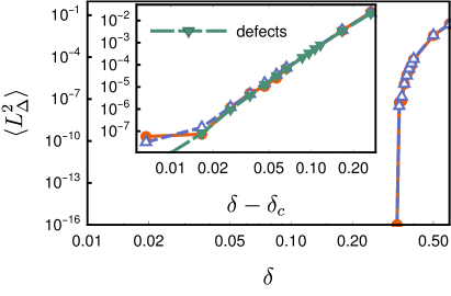
Figure S6: Residual energy per triangle of the MCM vs. $\delta$ for $L=12,24$ (circles, triangles) on a log-log scale. Inset: Close up close to the critical point compared to the direct evaluation of energy of ”defect” triangles with collinear spins.

Comparison of the correlations:

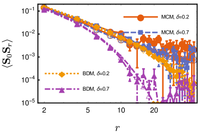
Figure S7: Comparison of the spin correlations in the ground state ensemble of $O(3)$ spins (filled symbols) to the self-consistent Gaussian apprximation (open symbols) at $T=0$ for both the bond-disordered model (BDM) and the maximal Coulomb model (MCM) in a system of linear size $L=48$ and disorder strengths $\delta=0.2,0.7$.

We next provide a comparison of the correlations in the ground state ensemble of $O(3)$-spins to the results of the self-consistent gaussian approximation (SCGA) for both the BDM and the MCM.

Fig. S7 shows the results for values of the disorder strength below the transition for $\delta=0.2$ and above for $\delta=0.7$ in a system with linear size $L=48$. We observe good agreement for both models and values of $\delta$ within the statistical errors of the ground state calculation. In addition, the correlations at large distances are seen to be exponentially suppressed for the BDM and decay algebraically for the MCM. Finally, we emphasise that the results of the SCGA have considerably less statistical noise and allow the study of larger system sizes as exploited in the main text.

Magnetic structure factor: Here, we compare the static magnetic structure factor of the BDM to the disorder-free system obtained from MC simulations at finite temperatures.

In Fig. S8 we observe that the BDM (panel a) does not develop the additional $\sqrt{3}\times\sqrt{3}$ peaks at low temperatures present for the disorder-free case (panel b). In addition, the BDM at a disorder strength $\delta$ with exponentially screened correlations compares well to the disorder-free case at a finite temperature $T^{*}\sim\delta^{2}$ which also exhibits screened correlations due to thermal fluctuations. This is demonstrated by the top left (panel a) for the BDM at $\delta=0.2$ and the bottom right (panel d) for the disorder free case at $T/J=0.02$.

(a)

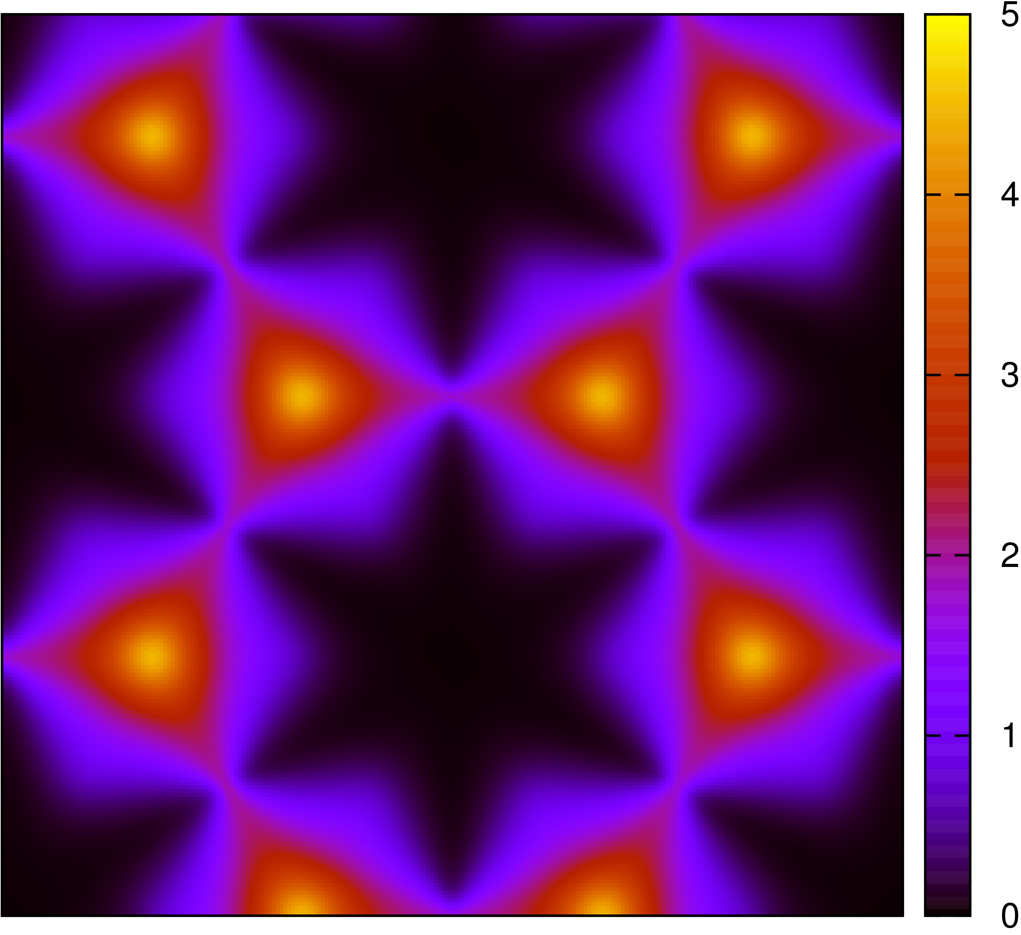
(b)

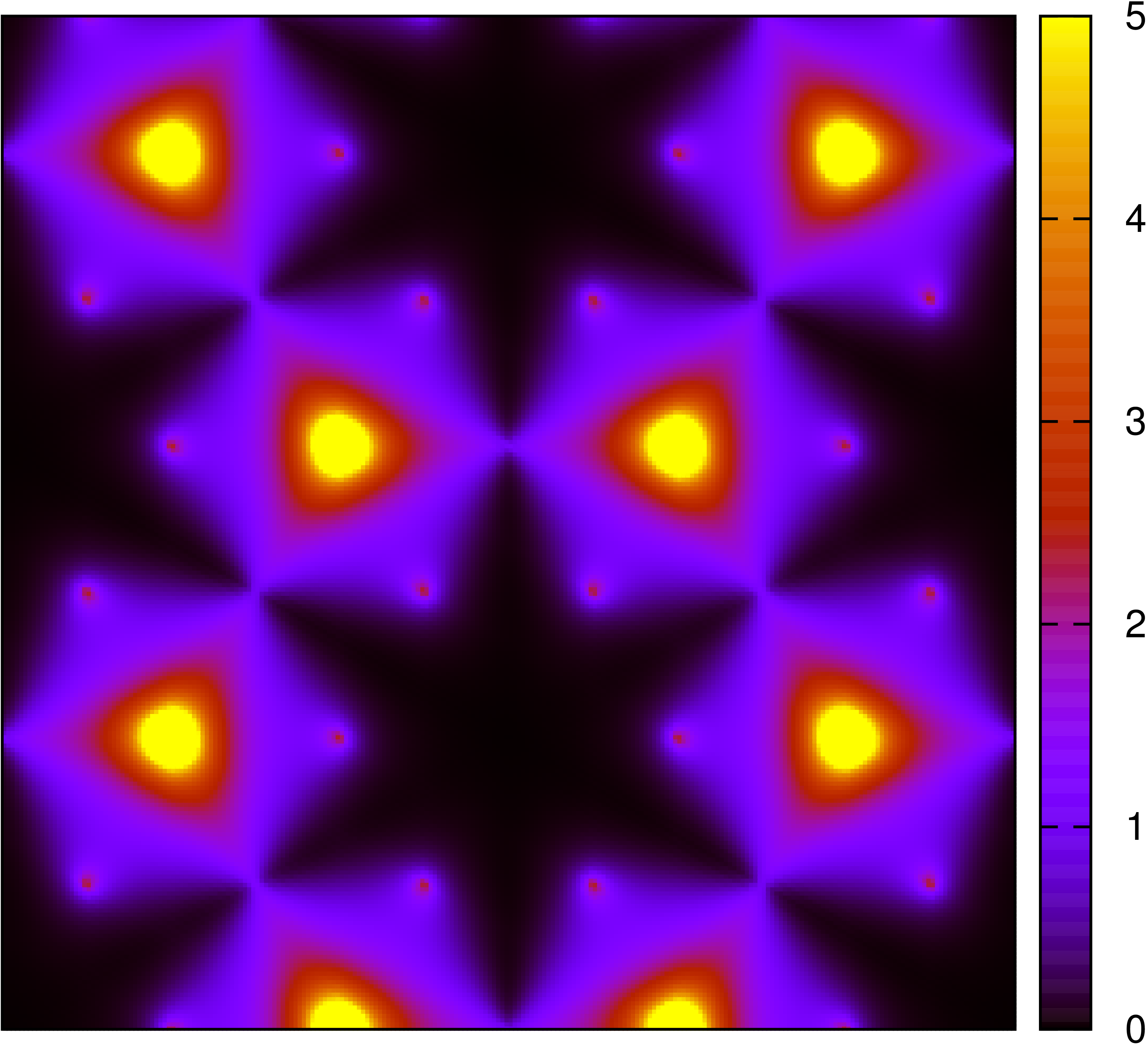
(c)

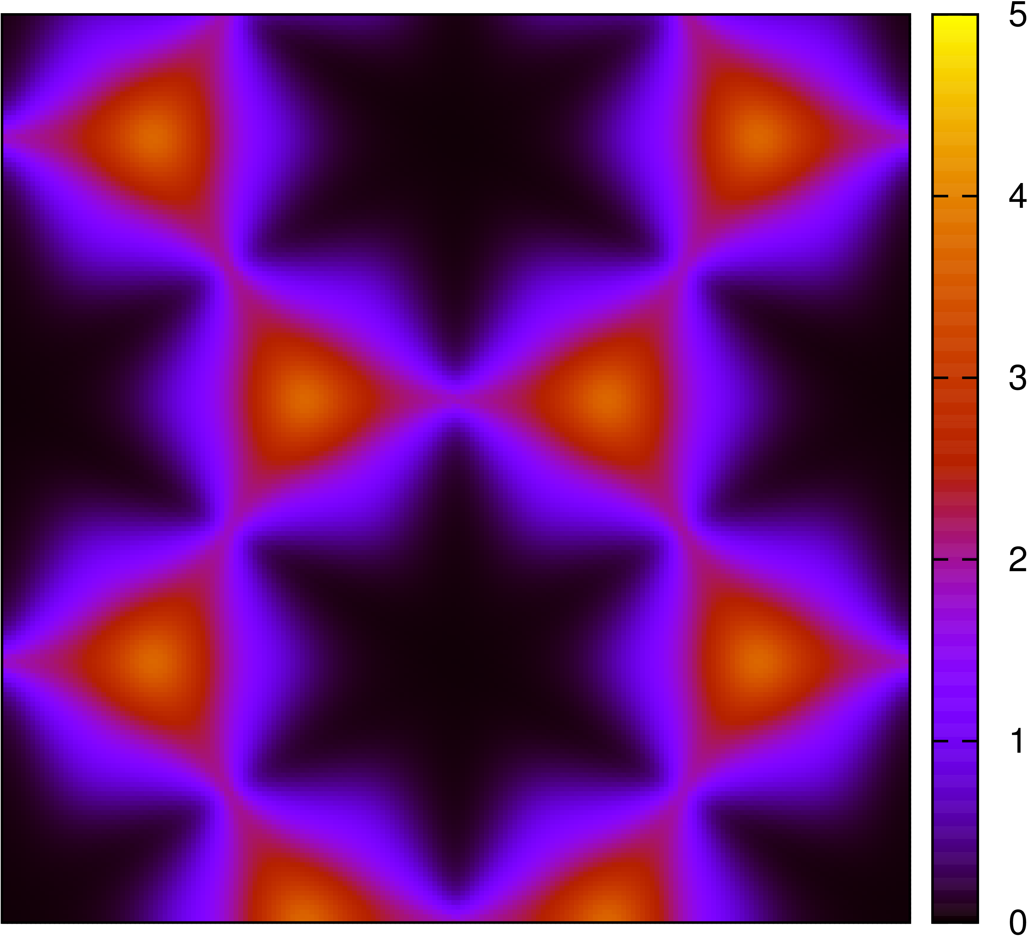
(d)

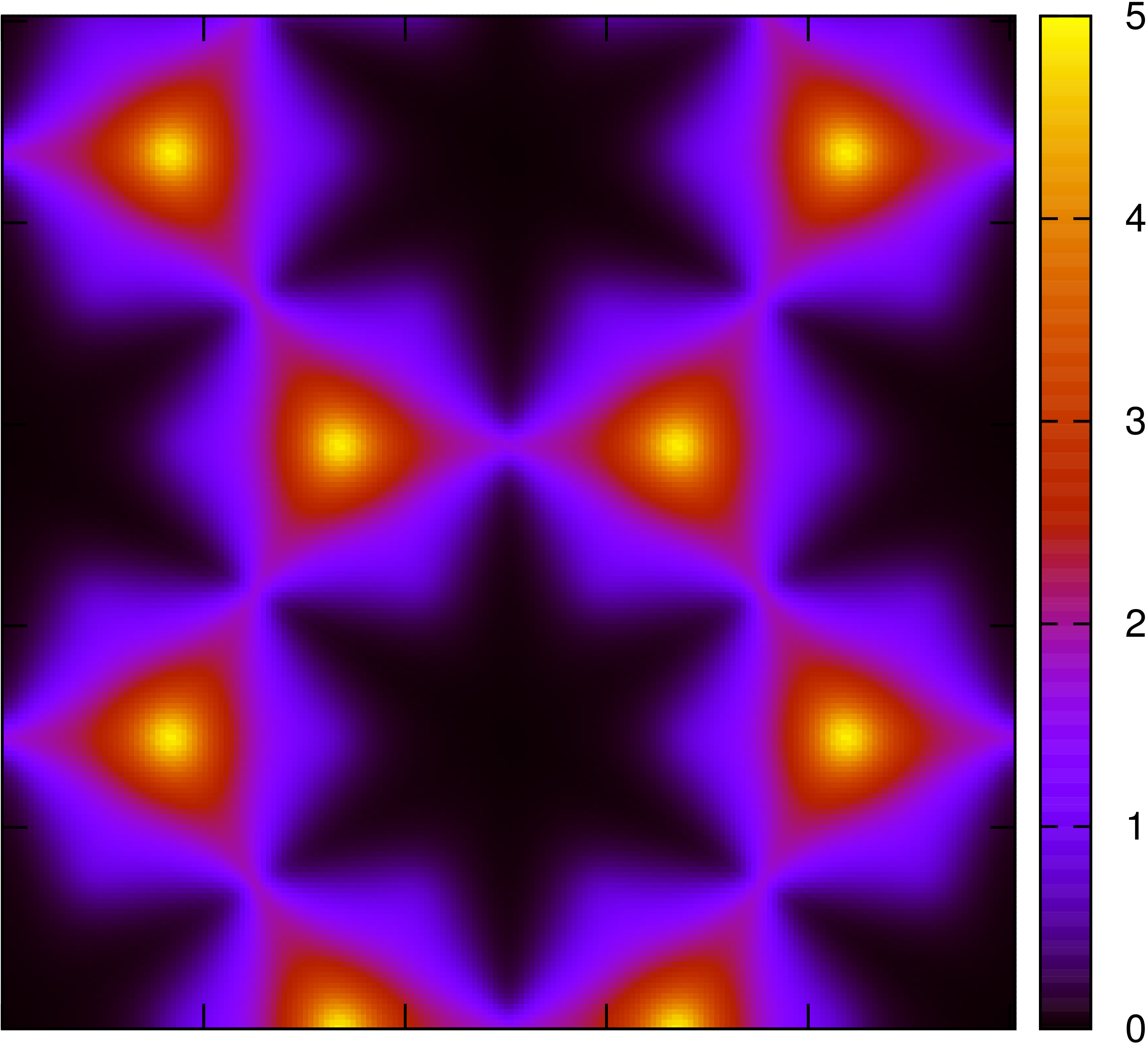
Figure S8: Comparison of the magnetic structure factor of the BDM to disorder-free kagome antiferromagnet in different temperature regimes. Region in the momentum space corresponds to $0\leq q_{x,y}\leq 8\pi$. Temperature in the top and bottom row $T/J=0.005$ and $T/J=0.02$ respectively. Left column for the BDM at disorder strength $\delta=0.2$, right column for the disorder-free model.

Spin glass transition:

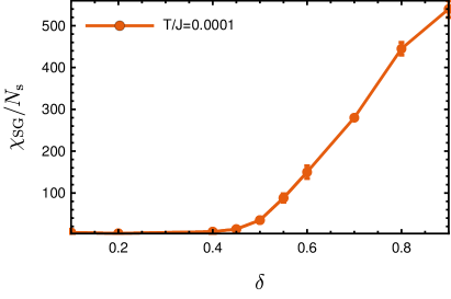
Figure S9: Extrapolated spin glass susceptibility $\chi_{\mathrm{SG}}$ vs. disorder strength for $T/J=10^{-4}$ from Monte-Carlo simulations for the BDM.

Fig. S9 shows the Monte-Carlo results for the spin glass susceptibility extrapolated to the thermodynamic limit based on systems with $L=4,\cdots,30$ at a fixed temperature $T/J=10^{-4}$ versus the disorder strength $\delta$. It clearly demonstrates the absence of spin glass correlations in the jammed-spin liquid and the existence of a spin glass for large $\delta$. However, we did not precisely determine the exact transition point into the spin glass $\delta_{\mathrm{SG}}$. In particular, we do not exclude the presence of an intermediate phase for $\delta_{c}<\delta<\delta_{SG}$.

II Checkerboard/planar pyrochlore lattice

In this section we provide a discussion of the physics of our model defined on the checkerboard/planar pyrochlore lattice for O$(2)$ spins.

We emphasise that in contrast to the kagome lattice on the planar pyrochlore lattice the bond-disordered model Eq.(1) (main text) is not equivalent to the model defined via scaling factors Eq.(2) (main text) as the former has 3 independent degrees of freedoms per spin (3 bond couplings per spin) and the latter only two scaling factors per spin. Thus, for a generic bond-disordered model it is not possible to write it as a sum of squares as for the kagome lattice.

Therefore, we will mainly discuss the MCM model in the following,

$$H=\frac{1}{2}\sum_{\alpha}{\bf{L}}_{\alpha}^{2},\quad\text{with}\quad{\bf{L}}_{\alpha}=\sum_{i\in\alpha}\gamma_{i\alpha}{\bf{S}}_{i}\,,$$ (S4)

where $\alpha$ now denotes the fully connected squares of the planar pyrochlore lattice illustrated in Fig. S10.

Analysis of a single square: We provide an estimate of the expected critical point based on the analysis of the constraint on a single square of the planar pyrochlore lattice.

The constraint

$$0=\sum_{i\in\Box}\gamma_{i}\mathbf{S}_{i}=\sum\gamma_{1}\mathbf{S}_{1}+\gamma_{2}\mathbf{S}_{2}+\gamma_{3}\mathbf{S}_{3}+\gamma_{4}\mathbf{S}_{4}$$ (S5)

clearly becomes unsatisfiable when $\gamma_{1}>\gamma_{2}+\gamma_{3}+\gamma_{4}$, where we assume the $\gamma_{i}$ to be ordered in magnitude. If we again choose $\gamma\in(1-\delta,1+\delta)$, and consider the extremal case $\gamma_{1}=1+\delta$, $\gamma_{2}=\gamma_{3}=\gamma_{4}=1-\delta$, this implies $\delta_{c}=1/2$.

Transfer matrix:

(a)

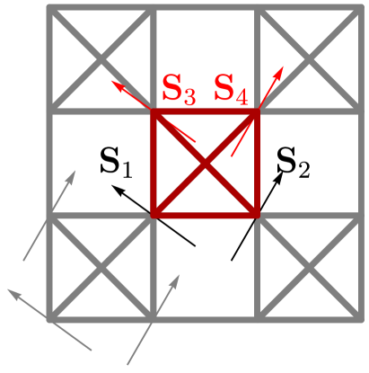
(b)

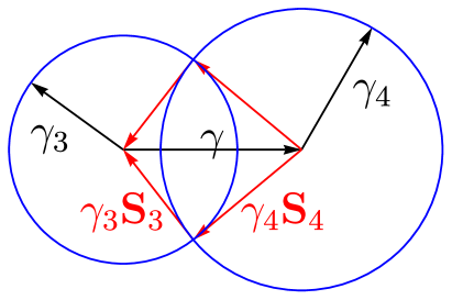
Figure S10: (a) Planar pyrochlore lattice, gray and black spins ($\mathbf{S}_{1}$, $\mathbf{S}_{2}$) are assumed known, red spins $\mathbf{S}_{3}$, $\mathbf{S}_{4}$ are to be determined. (b) Groundstate constraint in the bold central square, $\gamma=\left|\gamma_{1}\mathbf{S}_{1}+\gamma_{2}\mathbf{S}_{2}\right|$, allows generically two solutions for $\mathbf{S}_{3}$ and $\mathbf{S}_{4}$.

We continue with the transfer matrix argument as applicable to the planar pyrochlore lattice.

In the arrangement shown in Fig. S10(a) we have already chosen all spins to the left and below the black square of the planar pyrochlore lattice containing the known spins $\mathbf{S}_{1}$ and $\mathbf{S}_{2}$ and the unknown spins $\mathbf{S}_{3}$ and $\mathbf{S}_{4}$. We may rewrite the groundstate constraint in this square as

$$0=\sum_{i\in\Box}\gamma_{i}\mathbf{S}_{i}=\sum(\gamma_{1}\mathbf{S}_{1}+\gamma_{2}\mathbf{S}_{2})+\gamma_{3}\mathbf{S}_{3}+\gamma_{4}\mathbf{S}_{4}$$ (S6)

to recognise that it is equivalent to demanding that the vectors $(\gamma_{1}\mathbf{S}_{1}+\gamma_{2}\mathbf{S}_{2})$, $\gamma_{3}\mathbf{S}_{3}$, $\gamma_{4}\mathbf{S}_{4}$ form a closed triangle. As a triangle with three side lengths known is uniquely determined up to orientation, and we already know the orientation of one side, there remains a discrete choice between two configurations, related by mirror-reflection along the known side. We may then repeat this step to determine all spins in the next layer, and then throughout all layers to determine all spins in the lattice.

Ignoring potentially inconsistent configurations this yields an estimate of the number of groundstates $N_{gs}\sim 2^{N_{s}/2}$ as in every step we have 2 choices to fix 2 spins.

Constraint satisfaction: In this section we provide numerical evidence that the groundstates on the connected planar pyrochlore lattice indeed exactly satisfy the groundstate constraint up to the critical disorder strength $\delta_{c}=1/2$. In addition, we contrast these results to the truly bond-disordered model to show that the requirement that the model may be written as a sum of squares is indeed crucial to the existence of a “jammed” phase.

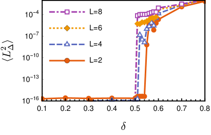
Figure S11: Residual energy $\langle L^{2}_{\Box}\rangle$ per square versus disorder strength for the MCM, Eq. S4, on the planar pyrochlore lattice for square systems with $L_{x}=L_{y}=2,4,6,8$

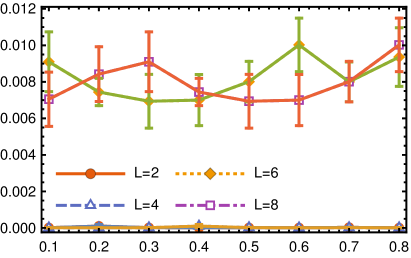
Figure S12: Residual energy $\langle L^{2}_{\Box}\rangle$ per square versus disorder strength for the bond-disordered model on the planar pyrochlore lattice for square systems with $L_{x}=L_{y}=2,4,6,8$

We show the resulting residual energies in Fig. S11. The results clearly demonstrate the transition at $\delta_{c}=1/2$ as expected from the analysis of an isolated square above. We emphasise that we expect the transition to also be continuous, and the jump only occurs as the lowest disorder strength simulated above the critical point is $\delta=0.51$, for which we expect a residual energy on the order of $\langle L^{2}_{\Box}\rangle\sim 10^{-5}$.

We may contrast this behaviour to that of the bond-disordered model shown in Fig. S12. Here we see a finite non-vanishing residual energy essentially independent of $\delta$ in the considered regime and there is no indication of any transition or a ”jammed “ phase in this model.

References

- Moessner and Ramirez [2006] R. Moessner and A. P. Ramirez, Physics Today 59, 24 (2006).
- Wannier [1950] G. H. Wannier, Phys. Rev. 79, 357 (1950).
- Anderson [1956] P. W. Anderson, Phys. Rev. 102, 1008 (1956).
- Shender et al. [1993] E. F. Shender, V. B. Cherepanov, P. C. W. Holdsworth, and A. J. Berlinsky, Phys. Rev. Lett. 70, 3812 (1993).
- Moessner and Berlinsky [1999] R. Moessner and A. J. Berlinsky, Phys. Rev. Lett. 83, 3293 (1999).
- Henley [2001] C. L. Henley, Can. J. Phys. 79, 1307 (2001).
- Bellier-Castella et al. [2001] L. Bellier-Castella, M. J. Gingras, P. C. Holdsworth, and R. Moessner, Canadian Journal of Physics 79, 1365 (2001).
- Saunders and Chalker [2007] T. E. Saunders and J. T. Chalker, Phys. Rev. Lett. 98, 157201 (2007).
- Andreanov et al. [2010] A. Andreanov, J. T. Chalker, T. E. Saunders, and D. Sherrington, Phys. Rev. B 81, 014406 (2010).
- Savary et al. [2011] L. Savary, E. Gull, S. Trebst, J. Alicea, D. Bergman, and L. Balents, Phys. Rev. B 84, 064438 (2011).
- Wang et al. [2007] F. Wang, A. Vishwanath, and Y. B. Kim, Phys. Rev. B 76, 094421 (2007).
- Chern et al. [2008] G.-W. Chern, R. Moessner, and O. Tchernyshyov, Phys. Rev. B 78, 144418 (2008).
- Roychowdhury et al. [2017] K. Roychowdhury, D. Zeb Rocklin, and M. J. Lawler, ArXiv e-prints (2017), arXiv:arXiv:1705.00015 [cond-mat.str-el] .
- Cépas and Canals [2012] O. Cépas and B. Canals, Phys. Rev. B 86, 024434 (2012).
- Sala et al. [2014] G. Sala, M. J. Gutmann, D. Prabhakaran, D. Pomaranski, C. Mitchelitis, J. B. Kycia, D. G. Porter, C. Castelnovo, and J. P. Goff, Nat Mater 13, 488 (2014).
- Sen and Moessner [2015] A. Sen and R. Moessner, Phys. Rev. Lett. 114, 247207 (2015).
- Savary and Balents [2017] L. Savary and L. Balents, Phys. Rev. Lett. 118, 087203 (2017).
- Benton et al. [2016] O. Benton, L. D. C. Jaubert, H. Yan, and N. Shannon, Nature Communications 7, 11572 (2016), arXiv:1510.01007 [cond-mat.str-el] .
- Rehn et al. [2017] J. Rehn, A. Sen, and R. Moessner, Phys. Rev. Lett. 118, 047201 (2017).
- Liu and Nagel [1998] A. J. Liu and S. R. Nagel, Nature 396, 21 (1998).
- O’Hern et al. [2003] C. S. O’Hern, L. E. Silbert, A. J. Liu, and S. R. Nagel, Phys. Rev. E 68, 011306 (2003).
- Liu and Nagel [2010] A. J. Liu and S. R. Nagel, Annual Review of Condensed Matter Physics 1, 347 (2010).
- Garanin [1996] D. A. Garanin, Phys. Rev. B 53, 11593 (1996).
- Chalker et al. [1992] J. T. Chalker, P. C. W. Holdsworth, and E. F. Shender, Phys. Rev. Lett. 68, 855 (1992).
- Ritchey et al. [1993] I. Ritchey, P. Chandra, and P. Coleman, Phys. Rev. B 47, 15342 (1993).
- Harris et al. [1992] A. B. Harris, C. Kallin, and A. J. Berlinsky, Phys. Rev. B 45, 2899 (1992).
- Moessner and Chalker [1998a] R. Moessner and J. T. Chalker, Phys. Rev. B 58, 12049 (1998a).
- Moessner and Chalker [1998b] R. Moessner and J. T. Chalker, Phys. Rev. Lett. 80, 2929 (1998b).
- Rehn et al. [2016] J. Rehn, A. Sen, K. Damle, and R. Moessner, Phys. Rev. Lett. 117, 167201 (2016).
- Garanin and Canals [1999] D. A. Garanin and B. Canals, Phys. Rev. B 59, 443 (1999).
- [31] See Supplemental Material at [URL will be inserted by publisher] for additional details on the enumeration searches, arguments for the continuity of the ground states as a function of disorder, explicit data on the energies of coplanar states, a comparison of the correlations for the MCM and the BDM in the SCGA calculation and additional MC data on the static structure factor and spin glass susceptibilities.
- Baxter [1970] R. J. Baxter, Journal of Mathematical Physics 11, 784 (1970).
- Stanley [1968] H. E. Stanley, Phys. Rev. 176, 718 (1968).
- Huse and Rutenberg [1992] D. A. Huse and A. D. Rutenberg, Phys. Rev. B 45, 7536 (1992).
- Kane and Lubensky [2014] C. L. Kane and T. C. Lubensky, Nat Phys 10, 39 (2014).
- Lawler [2016] M. J. Lawler, Phys. Rev. B 94, 165101 (2016).
- Zhitomirsky [2008] M. E. Zhitomirsky, Phys. Rev. B 78, 094423 (2008).
- Chern and Moessner [2013] G.-W. Chern and R. Moessner, Phys. Rev. Lett. 110, 077201 (2013).
- Conlon and Chalker [2009] P. H. Conlon and J. T. Chalker, Phys. Rev. Lett. 102, 237206 (2009).
- Robert et al. [2008] J. Robert, B. Canals, V. Simonet, and R. Ballou, Phys. Rev. Lett. 101, 117207 (2008).
- Taillefumier et al. [2014] M. Taillefumier, J. Robert, C. L. Henley, R. Moessner, and B. Canals, Phys. Rev. B 90, 064419 (2014).
- Keren [1995] A. Keren, International Conference on Magnetism 140, 1493 (1995).
- Halperin and Saslow [1977] B. I. Halperin and W. M. Saslow, Phys. Rev. B 16, 2154 (1977).
- Rehn et al. [2015] J. Rehn, A. Sen, A. Andreanov, K. Damle, R. Moessner, and A. Scardicchio, Phys. Rev. B 92, 085144 (2015).
- Wills and Harrison [1996] A. S. Wills and A. Harrison, J. Chem. Soc., Faraday Trans. 92, 2161 (1996).
- Bisson and Wills [2008] W. G. Bisson and A. S. Wills, Journal of Physics: Condensed Matter 20, 452204 (2008).
- Wills et al. [2000a] A. S. Wills, A. Harrison, C. Ritter, and R. I. Smith, Phys. Rev. B 61, 6156 (2000a).
- Wills et al. [2000b] A. S. Wills, V. Dupuis, E. Vincent, J. Hammann, and R. Calemczuk, Phys. Rev. B 62, R9264 (2000b).
- Dupuis et al. [2002] V. Dupuis, E. Vincent, J. Hammann, J. E. Greedan, and A. S. Wills, Journal of Applied Physics 91, 8384 (2002).
- Ladieu et al. [2004] F. Ladieu, F. Bert, V. Dupuis, E. Vincent, and J. Hammann, Journal of Physics: Condensed Matter 16, S735 (2004).
- [51] V. Lubchenko and P. G. Wolynes, 1710.02857v1 .
- [52] Q. Wu, T. Bertrand, M. D. Shattuck, and C. S. O’Hern, 1710.01438v1 .
- Franz et al. [2017] S. Franz, G. Parisi, M. Sevelev, P. Urbani, and F. Zamponi, SciPost Phys. 2, 019 (2017).

References

- Zhou and Barjaktarevic [2008] Huan-Qiang Zhou and John Paul Barjaktarevic, “Fidelity and quantum phase transitions,” Journal of Physics A: Mathematical and Theoretical 41, 412001 (2008).
- Gu [2010] Shi-Jian Gu, “Fidelity approach to quantum phase transitions,” International Journal of Modern Physics B 24, 4371–4458 (2010).