Relativistic corrections to the static energy in terms of Wilson loops at weak coupling

Abstract

We consider the ${\mathcal{O}}(1/m)$ and the spin-independent momentum-dependent ${\mathcal{O}}(1/m^{2})$ quasi-static energies of heavy quarkonium (with unequal masses). They are defined nonperturbatively in terms of Wilson loops. We determine their short-distance behavior through ${\cal O}(\alpha^{3})$ and ${\cal O}(\alpha^{2})$, respectively. In particular, we calculate the ultrasoft contributions to the quasi-static energies, which requires the resummation of potential interactions. Our results can be directly compared to lattice simulations. In addition, we also compare the available lattice data with the expectations from effective string models for the long-distance behavior of the quasi-static energies.

1 Introduction

The near-threshold dynamics of quark-antiquark systems with large masses can be described by a properly generalized nonrelativistic (NR) Schrödinger equation. Such equation can be derived from first principles using effective field theories (EFT’s) like potential NRQCD (pNRQCD) Pineda:1997bj ; Brambilla:1999xf (for reviews see Brambilla:2004jw ; Pineda:2011dg ). This EFT systematically exploits the nonrelativistic scale hierarchy $m\gg mv\gg mv^{2}\ldots\,$, where $v$ is the heavy-quark velocity in the center of mass frame. In the case of unequal heavy quark masses, we will assume $m_{1}\sim m_{2}\sim m$.

In this paper we will mostly work in the weak-coupling regime, where the EFT can be schematically summarized as

$$\,\left.\begin{array}[]{ll}&\left(i\partial_{0}-\frac{{\bf p}^{2}}{2m_{r}}-V_{s}(r)\right)\phi({\mathbf{r}})=0\\ &+\;\text{interactions with other low-energy}\\ &\hskip 7.96674pt\text{ degrees of freedom}\end{array}\right\}\text{pNRQCD}\,.$$ (4)

Here, $m_{r}=m_{1}m_{2}/(m_{1}+m_{2})$, $\phi({\mathbf{r}})$ represents the quarkonium wave function, ${\mathbf{p}}$ is the momentum operator conjugate to the distance vector ${\mathbf{r}}$ between the heavy quarks and $V_{s}$ is the color-singlet potential. We denote the color-octet potential by $V_{o}$. The potential $V_{s}$ consists of the static potential $V^{(0)}$ and its relativistic corrections, which are suppressed by inverse powers of the heavy quark masses. For the general case of unequal masses we have

$$V_{s}= V^{(0)}+\frac{V^{(1,0)}}{m_{1}}+\frac{V^{(0,1)}}{m_{2}}$$

$$+ \frac{V^{(2,0)}}{m_{1}^{2}}+\frac{V^{(0,2)}}{m_{2}^{2}}+\frac{V^{(1,1)}}{m_{1}m_{2}}+\cdots,$$ (5)

where the spin-independent (SI) $1/m^{2}$ potentials are

$$V^{(2,0)}_{SI}= \frac{1}{2}\left\{{\bf p}_{1}^{2},V_{{\bf p}^{2}}^{(2,0)}(r)\right\}+V_{r}^{(2,0)}(r)+V_{{\bf L}^{2}}^{(2,0)}(r)\frac{{\bf L}_{1}^{2}}{r^{2}}\,,$$ (6)

$$V^{(0,2)}_{SI}= \frac{1}{2}\left\{{\bf p}_{2}^{2},V_{{\bf p}^{2}}^{(0,2)}(r)\right\}+V_{r}^{(0,2)}(r)+V_{{\bf L}^{2}}^{(0,2)}(r)\frac{{\bf L}_{2}^{2}}{r^{2}}\,,$$ (7)

$$V^{(1,1)}_{SI}= -\frac{1}{2}\left\{{\bf p}_{1}\cdot{\bf p}_{2},V_{{\bf p}^{2}}^{(1,1)}(r)\right\}+V_{r}^{(1,1)}(r)$$

$$-V_{{\bf L}^{2}}^{(1,1)}(r)\frac{({\bf L}_{1}\cdot{\bf L}_{2}+{\bf L}_{2}\cdot{\bf L}_{1})}{2r^{2}}\,,$$ (8)

with ${\bf L}_{1}\equiv{\bf r}\times{\bf p}_{1}$, ${\bf L}_{2}\equiv{\bf r}\times{\bf p}_{2}$, and ${\bf p}_{1}$, ${\bf p}_{2}$ being the momenta of the heavy quarks in the center of mass frame. In what follows we will not consider spin-dependent potentials.

The potential in Eq. (4) is obtained by matching pNRQCD to NRQCD Caswell:1985ui ; Bodwin:1994jh . There are several ways to perform this matching in practice. In general, the resulting expressions for the relativistic corrections to the potential at different orders in the $1/m$ expansion, also referred to as (higher order) ‘potentials’, depend on the matching scheme. Nevertheless physical observables are of course unaffected. For a detailed discussion see Ref. Peset:2015vvi .

In this paper we focus on the potentials obtained from Wilson-loop matching. This scheme requires certain gauge invariant NRQCD and pNRQCD Green functions in position space to be equal at a given order in $1/m$. On the NRQCD side these Green functions correspond to rectangular Wilson loops with chromo-electric/-magnetic field operator insertions. The potentials are Wilson coefficients of pNRQCD operators. Appropriate correlation functions of these operators are then matched onto the Wilson loops to determine the potentials. For details on the Wilson-loop matching we refer to Refs. Brambilla:2000gk ; Pineda:2000sz . In the static limit, i.e. at lowest order in $1/m$, the potential reduces to the original Wilson-loop expression for the static potential $V^{(0)}$ Wilson:1974sk . The Wilson-loop expression for the $1/m$ potential was obtained in Ref. Brambilla:2000gk , for the $1/m^{2}$ potential without light fermions in Ref. Pineda:2000sz , and including light fermions in Ref. Peset:2015vvi . The corresponding expressions in terms of Wilson loops for the SI momentum-dependent $1/m^{2}$ potentials, $V_{{{\mathbf{p}}}^{2}}$ and $V_{{{\mathbf{L}}}^{2}}$, were first derived in Ref. Barchielli:1986zs . The latter reference however missed the $1/m$ potential, which we also study in this paper.

Only (off-shell) soft modes, i.e. those modes with energies and momenta of order $1/r$, contribute to the potential in the Wilson loop scheme. This is achieved by Taylor expanding in powers of $1/m$ before integrating over the gauge and light-quark degrees of freedom. Thus, soft modes are properly accounted for, but ultrasoft modes still need to be eliminated. At weak-coupling this is achieved by evaluating the Wilson loops strictly in perturbation theory. Hence, the only physical scale left in the Wilson-loop calculation of the potential is $1/r$.

Still, the definition of the potential in terms of Wilson loops naturally suggests its generalization beyond perturbation theory. We will refer to this generalized potential as the quasi-static energy. To distinguish it from the potential $V$ we will use the symbol $E$ for the quasi-static energy. The definition in terms of Wilson loops has the same form for both quantities, but $E$ is evaluated nonperturbatively, for instance through lattice simulations. Varying the distance $r$ allows us to move continuously from the extreme weak-coupling limit ($r\rightarrow 0$) to the strong-coupling regime ($r\rightarrow\infty$) of the quasi-static energies. They are therefore ideal observables to study the interplay between both regimes in a controlled manner.

At long distances, the quasi-static energies are suitable for the study of nonperturbative QCD dynamics, e.g. by comparing different models with lattice simulations. In this regime there is a direct connection to the strong-coupling version of pNRQCD, as (omitting possible ultrasoft modes of chiral origin and treating $V^{(0)}$ as small compared to the soft scale) the total quasi-static energy corresponds to the Hamiltonian operator that describes the heavy quarkonium bound state, see Refs. Brambilla:2000gk ; Pineda:2000sz . The determination of the quasi-static energy might therefore, for example, enable predictions of the higher excitations of bottomonium and charmonium. For a recent attempt in this direction see Ref. Brambilla:2014eaa .

Even at short distances, the regime we will focus on in this paper, the behavior of the quasi-static energies cannot be obtained from a strictly perturbative computation in the strong coupling $\alpha\equiv\alpha_{\rm s}$ alone. The reason is that the so-called ultrasoft scale $\Delta V\equiv V^{(0)}_{o}-V^{(0)}\simeq C_{A}\alpha/(2r)\ll 1/r$ is generated dynamically by the exchange of an arbitrary number of Coulomb gluons. Including the ultrasoft effects requires a proper resummation of such potential interactions. Typically this is done with the help of EFTs, but it can also be done using a diagrammatic approach, as we will show. Thus, in addition to the perturbative soft part $V_{s}$, the quasi-static energy $E_{s}$ also includes ultrasoft contributions, which are inaccessible in perturbation theory, even at weak coupling. Therefore it differs from the potential, which enters the Schrödinger equation that describes heavy quarkonium dynamics. Still, both objects are obtained by expanding in powers of $1/m$ before the integration over the relevant gauge or light-quark dynamical modes.

In Ref. Peset:2015vvi , we determined the soft contributions to the quasi-static energies up to $\mathcal{O}(\alpha^{3}/m)$ and $\mathcal{O}(\alpha^{2}/m^{2})$. For the complete results at short distances we also need the ultrasoft contributions. We will compute them in this paper for the $1/m$ and the SI momentum-dependent $1/m^{2}$ quasi-static energies ($E_{{{\mathbf{p}}}^{2}}$, $E_{{{\mathbf{L}}}^{2}}$). Adding soft and ultrasoft contributions we obtain the $1/m$ quasi-static energy with ${\cal O}(\alpha^{3})$ precision and $E_{{{\mathbf{p}}}^{2}}$, $E_{{{\mathbf{L}}}^{2}}$ with ${\cal O}(\alpha^{2})$ precision. We also discuss the possible resummation of large logarithms for these quantities.

Our results can be directly confronted with the most recent lattice data from Refs. Koma:2006si ; Koma:2007jq ; Koma:2009ws . One motivation for such a comparison is to perform quantitative checks of ultrasoft effects. The static energy $E^{(0)}$ starts to be sensitive to the ultrasoft scale only at ${\cal O}(\alpha^{4})$, i.e. N³LO Appelquist:1977es ; Brambilla:1999qa . The high $\alpha$ suppression makes it difficult to study ultrasoft physics with this observable. For the quasi-static energies $E^{(1,0)}$, $E^{(0,1)}$ and $E^{(1,1)}$ ultrasoft effects already contribute at NLO, for $E^{(2,0)}$ and $E^{(0,2)}$ even at leading non-vanishing order. They are therefore a good testing ground for both the ultrasoft physics and the reliability of the weak coupling prediction at a given distance $r$. This is important for several reasons. For example to give support to perturbative analyses of the heavy quarkonium spectrum that include ultrasoft contributions at weak coupling Penin:2002zv ; Ayala:2014yxa ; Kiyo:2015ufa . It is also crucial for determinations of the strong coupling constant $\alpha$ from lattice simulations of the static energy Bazavov:2012ka , as they rely on the correct treatment of ultrasoft effects over the whole range of (short) distances they probe. Finally, we would also like to remark that in ${\cal N}=4$ supersymmetric Yang-Mills theories the static energy $E^{(0)}$ is also sensitive to ultrasoft effects starting at NLO, see Erickson:1999qv ; Pineda:2007kz ; Stahlhofen:2012zx ; Prausa:2013qva . Preliminary results from lattice simulations for this quantity have been reported in Schaich:2016jus . They qualitatively agree with the perturbative predictions (including the ultrasoft contributions) at small distances. A more detailed analysis would however be welcome.

2 The quasi-static energy and its relativistic corrections

We will use the following definitions for the Wilson-loop operators and their vacuum expectation values. The angular brackets $\langle\dots\rangle$ stand for the average value over the QCD action, $W_{\Box}$ for the rectangular static Wilson loop of dimensions $r\times T_{W}$,

$$W_{\Box}\equiv{\rm P}\exp\left\{{\displaystyle-ig\oint_{r\times T_{W}}\!\!dz^{\mu}A_{\mu}(z)}\right\},$$ (9)

and

$$\langle\!\langle\dots\rangle\!\rangle\equiv\frac{\langle{\rm P}\dots W_{\Box}\rangle}{\langle W_{\Box}\rangle}\,,$$ (10)

where P is the path-ordering operator. Moreover, we define the connected Wilson loop average

$$\langle\!\langle O_{1}(t_{1})O_{2}(t_{2})\rangle\!\rangle_{c}=\langle\!\langle O_{1}(t_{1})O_{2}(t_{2})\rangle\!\rangle-\langle\!\langle O_{1}(t_{1})\rangle\!\rangle\langle\!\langle O_{2}(t_{2})\rangle\!\rangle$$ (11)

of operator insertions $O_{1}$, $O_{2}$ in the Wilson (static quark) lines at times $t_{1}$ and $t_{2}$ with $T_{W}/2\geq t_{1}\geq t_{2}\geq-T_{W}/2$. We also define the short-hand notation

$$\lim_{T\rightarrow\infty}\equiv\lim_{T\rightarrow\infty}\lim_{T_{W}\rightarrow\infty}\,,$$ (12)

where $T_{W}$ is the time length of the Wilson loop and $T$ the upper limit of the time integrals in the definitions below. By taking first the $T_{W}\rightarrow\infty$ limit, the averages $\langle\!\langle\dots\rangle\!\rangle$ become independent of $T_{W}$ and thus invariant under global time translations, see Ref. Pineda:2000sz for details.

The total color-singlet quasi-static energy is defined as the sum of the kinetic terms and the nonperturbative generalization of the potential in terms of Wilson loops. It reads

$$E_{s}({\bf r},{\bf p},{\bf P}_{\bf R},{\bf S}_{1},{\bf S}_{2})=$$

$$\qquad\frac{{\bf p}^{2}}{2\,m_{\rm r}}+\frac{{\bf P}_{\bf R}^{2}}{2\,M}+E^{(0)}+\frac{E^{(1,0)}}{m_{1}}+\frac{E^{(0,1)}}{m_{2}}$$

$$\qquad+\frac{E^{(2,0)}}{m_{1}^{2}}+\frac{E^{(0,2)}}{m_{2}^{2}}+\frac{E^{(1,1)}}{m_{1}m_{2}}+{\mathcal{O}}\bigg{(}\frac{1}{m^{3}}\bigg{)}\,,$$ (13)

where ${\bf P}_{\bf R}$ is the center of mass momentum operator, ${\mathbf{p}}=-i\nabla_{\mathbf{r}}$, $M=m_{1}+m_{2}$, the reduced mass $m_{r}=m_{1}m_{2}/M$, and

$$E^{(0)}(r)=\lim_{T\to\infty}\frac{i}{T}\ln\langle W_{\Box}\rangle$$ (14)

is the static energy Wilson:1974sk . The formal definitions for the higher order quasi-static energies to ${\mathcal{O}}(1/m)$ can be found in Ref. Brambilla:2000gk and to ${\mathcal{O}}(1/m^{2})$ in Refs. Pineda:2000sz ; Peset:2015vvi . Here we recall the ones relevant for the present work. At ${\mathcal{O}}(1/m)$ we have

$$E^{(1,0)}(r)=-\frac{1}{2}\lim_{T\rightarrow\infty}\int_{0}^{T}dt\,t\,\langle\!\langle g{\bf E}_{1}(t)\cdot g{\bf E}_{1}(0)\rangle\!\rangle_{c}\,.$$ (15)

The SI momentum-dependent $1/m^{2}$ potentials are parametrized in complete analogy to Eqs. (6)-(8) and given by

$$E_{{\bf p}^{2}}^{(2,0)}(r )=\frac{i}{2}{\hat{\bf r}}^{i}{\hat{\bf r}}^{j}\lim_{T\rightarrow\infty}\int_{0}^{T}dt\,t^{2}\langle\!\langle g{\bf E}_{1}^{i}(t)g{\bf E}_{1}^{j}(0)\rangle\!\rangle_{c}\,,$$ (16)

$$E_{{\bf L}^{2}}^{(2,0)}(r) =\frac{i}{2(d-1)}\left(\delta^{ij}-d{\hat{\bf r}}^{i}{\hat{\bf r}}^{j}\right)$$

$$\times\lim_{T\rightarrow\infty}\int_{0}^{T}dt\,t^{2}\langle\!\langle g{\bf E}_{1}^{i}(t)g{\bf E}_{1}^{j}(0)\rangle\!\rangle_{c}\,,$$ (17)

$$E_{{\bf p}^{2}}^{(1,1)}(r) =i\,{\hat{\bf r}}^{i}{\hat{\bf r}}^{j}\lim_{T\rightarrow\infty}\int_{0}^{T}dt\,t^{2}\langle\!\langle g{\bf E}_{1}^{i}(t)g{\bf E}_{2}^{j}(0)\rangle\!\rangle_{c}\,,$$ (18)

$$E_{{\bf L}^{2}}^{(1,1)}(r) =\frac{i}{d-1}\left(\delta^{ij}-d{\hat{\bf r}}^{i}{\hat{\bf r}}^{j}\right)$$

$$\times\lim_{T\rightarrow\infty}\int_{0}^{T}dt\,t^{2}\langle\!\langle g{\bf E}_{1}^{i}(t)g{\bf E}_{2}^{j}(0)\rangle\!\rangle_{c}\,,$$ (19)

where $d=D-1=3+2\epsilon$, ${\hat{\bf r}}={\bf r}/r$ and ${\mathbf{E}}_{n}$ is the chromo-electric field-strength operator to be inserted on the Wilson line associated with the static quark ($n=1$) or on the Wilson line associated with the static antiquark ($n=2$). The coupling $g$ in the above expressions will be replaced by the bare coupling $g_{B}$ in the actual calculations carried out in the next section. We do not consider spin (${\bf S}_{1,2}$)-dependent or momentum (${\mathbf{p}}_{1,2}$)-independent quasi static energies in this paper.

The potential $V_{s}$, which enters the Schrödinger equation that describes heavy quarkonium dynamics, is determined by expanding in powers of $1/m$ before integrating over any gauge and light-quark dynamical degrees of freedom. For the ultrasoft scales this implies $\Delta V\gg{\mathbf{p}}^{2}/m$. Concerning the ultrasoft contributions to the energy of a physical bound state of dynamical heavy quarks such a $1/m$ expansion would be incorrect, as according to the Virial theorem $\Delta V\sim{\mathbf{p}}^{2}/m$. This is the reason why ultrasoft modes are removed from the potential. They are retained in the quasi-static energy, which can therefore be (formally) regarded as the heavy quarkonium energy in the quasi-static limit: $\Delta V\gg{\mathbf{p}}^{2}/m$.

The relation between the total (singlet) quasi-static energy $E_{s}$ and the potential in the Wilson loop scheme $V_{s,W}$ is

$$E_{s}(r)=V_{s,W}(r)+\delta E_{s,{\rm US}}(r)\,,$$ (20)

where $\delta E_{s,{\rm US}}$ denotes the ultrasoft contribution to the quasi-static energy. The analogous splitting into the corresponding (soft) potential and ultrasoft contribution is understood for each of the quasi-static energies $E^{(\ldots)}_{\ldots}$ in Eqs. (14)-(2).

In order to compute the potential $V_{s,W}(r)$ in perturbation theory, the ultrasoft contribution must be completely subtracted. The latter can be achieved in dimensional regularization by expanding in the ultrasoft scale $\Delta V$ before performing the loop integrations. As $\Delta V\propto\alpha$ this means we simply have to ensure a strictly perturbative calculation in $\alpha$. Thus, only the soft scale $1/r$ is left and the loop integrals become homogeneous in that scale. The potentials then take the form of a power series in $\alpha\propto g^{2}$ (and, eventually, in $\Delta V$, when working beyond the order we work at in this paper). In summary we have,

$$V_{s,W}(r)=E_{s}(r)|_{\rm soft}\,.$$ (21)

We have presented the results for the potential $V_{s,W}$ up to ${\mathcal{O}}(\alpha^{3}/m)$ and ${\mathcal{O}}(\alpha^{2}/m^{2})$ in Ref. Peset:2015vvi .

In the weak-coupling regime ultrasoft degrees of freedom, with energies and momenta of order $\Delta V\equiv V^{(0)}_{o}-V^{(0)}\sim C_{A}\alpha/r$, contribute to the quasi-static energies through $\delta E_{s,{\rm US}}$. These contributions to the Wilson loops correspond to the contributions from the lower (ultrasoft) energy regions in an asymptotic expansion of the loop integrations according to the method of regions Beneke:1997zp . This implies that (some of) the loop integrals are sensitive to the ultrasoft scale. In analogy to Eq. (21) we write

$$\delta E_{s,{\rm US}}(r)=E_{s}(r)|_{\rm US}\,.$$ (22)

Next, we explain how to compute $\delta E_{s,{\rm US}}$ in detail.

2.1 Ultrasoft calculation

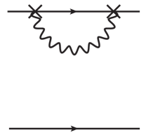
Figure 1: Connected (2-Wilson-line irreducible) diagrams with one ultrasoft gluon exchange contributing to $E_{\rm US}^{(2,0)}$ and $E_{\rm US}^{(1,0)}$. Left-right mirror graphs are understood. Dotted lines represent the $A^{0}$, wiggled lines the ${\mathbf{A}}$ components of a gluon. The time axis in these diagrams extends from left to right. The crosses symbolize the chromo-electric operator insertions at times $0$ and $t$ on the upper Wilson line (solid). Vertical lines are associated with potential gluons. The ultrasoft gluon is depicted as diagonal, horizontal or curvy line. We adopt the NRQCD convention for the fermion flow (little arrows on the Wilson lines) explained in Figure 3. Diagrams $(1b)$, $(2c)$, $(3e)$, $(3f)$, $(3g)$ vanish in Coulomb gauge as they are proportional to scaleless integrals.

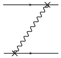
Figure 2: Connected diagrams with one ultrasoft gluon exchange contributing to $E_{\rm US}^{(1,1)}$. Left-right mirror graphs are understood. As explained in the text, the diagrams are in one-to-one correspondence, and in fact equal, to the ones of Figure 1.

In Ref. Peset:2015vvi we obtained the NLO soft color-singlet contribution to Eqs. (15)-(2). In contrast, the ultrasoft contribution to the NLO quasi-static energies cannot be calculated within conventional perturbation theory. As the ultrasoft scale is only generated dynamically, it requires the resummation of LO potential (Coulomb) interactions.

In the Wilson loop calculation the ultrasoft scale $\Delta V\sim C_{A}\alpha/r$ is generated by the ratio of the resummed (exponential) LO expressions for the rectangular color-octet Wilson loop in the numerator and the color-singlet Wilson loop in the denominator in the definition of the quasi-static energies in Eqs. (15)-(2), cf. Eq. (10). This leads to a factor $\exp(-i\Delta Vt)$, where $t$ is the (positive) time interval spanned by a (ultrasoft) gluon exchange between the quarks, in the otherwise perturbative calculation. As will be explained below this exponential factor can be effectively treated as a position-space quark-antiquark pair propagator in our diagrammatic approach to the ultrasoft computation, similar to the singlet and octet (bound-state) propagators in pNRQCD Pineda:1997bj ; Brambilla:1999xf .

To achieve a clean and systematic separation from the soft contribution within dimensional regularization, we follow the method of regions Beneke:1997zp . That is, we assign a definite energy and momentum scaling to the degrees of freedom involved in the ultrasoft calculation and consistently expand according to the power counting. In our case the relevant degrees of freedom are the ultrasoft gluon with four-momentum $q^{\mu}\sim\Delta V$ and potential gluons with energy $k_{0}\sim\Delta V$ and three-momentum ${\mathbf{k}}\sim 1/r\gg\Delta V$. The Wilson lines themselves can be interpreted as static (anti)quarks interacting with both types of gluons. Modes with soft energies $\sim 1/r$ are insensitive to the ultrasoft scale and therefore decouple from the ultrasoft modes. They are not needed for the ultrasoft contribution to the NLO quasi-static energies. In this calculation only one ultrasoft gluon and a (infinite) number of potential gluons are involved. The couplings of the ultrasoft gluon yield a factor $\alpha$ relative to the LO, whereas any additional potential gluon exchange does not change the power counting.

To compute the correlator $\langle\langle{\bf E}_{a}^{i}(t){\bf E}_{b}^{j}(0)\rangle\rangle_{c}$ with two chromo-electric field operators ($a,b\in\{1,2\}$) we use a (non-standard) diagrammatic approach. The relevant (‘connected’) diagrams for the ultrasoft part of the quasi-static energies in Eqs. (15)-(2) are displayed in Figures 1 and 2. Vertical lines represent potential gluons, which do not propagate in time (after expansion in the ultrasoft momentum). Potential gluon interactions that will be resummed are not displayed. We will come back to this later. The ultrasoft gluon is depicted as horizontal, diagonal or curvy line. Before we comment on the selection criteria for these diagrams, we describe how to construct and evaluate them.

The procedure is as follows. We first locate the vertices of the ultrasoft and potential gluons at specific times. As a consequence there is a priori no energy conservation at these vertices. The two vertices for the chromo-electric field operator insertions on the static quark (Wilson) lines are fixed at times $0$ and $t$, respectively. The time coordinates of the other vertices have to be integrated over. The energies in the potential gluon propagators are expanded out and do not contribute at NLO. The integration over these energies can therefore be carried out immediately yielding delta functions of time intervals. Many of the time integrations can now be performed trivially. The result is that vertices connected by potential gluons are all located at the same time. This has been indicated already in our graphs in Figures 1 and 2, where time proceeds from left to right.

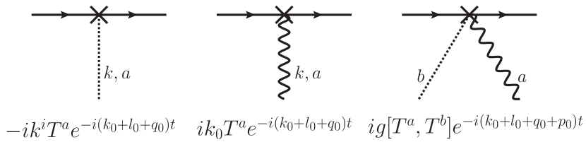
Figure 3: Feynman rules for an ${\bf E}^{i}(t)$ operator insertion (denoted by a cross in the diagram) on a static quark (Wilson) line. Dotted and wavy lines represent $A_{0}$ and $\bf A$ gluons, respectively. All momenta ($k,l,q,p$) are incoming. Note that, in contrast to the usual convention for Wilson lines, we treat the antiquark (lower Wilson line) as a particle living in the anti-representation of $SU(3)$, i.e. the fermion flow (little arrows) of the antiquark is the same as for the quark. The corresponding Feynman rules for the antiquark are then obtained by replacing $g\rightarrow-g$ and $T^{a}\rightarrow(T^{a})^{T}$.

The vertices for the chromo-electric operator insertions are the same as the ones given in Ref. Peset:2015vvi and shown in Figure 3. For the Wilson line interaction of an $A^{0}$ gluon, the quark and gluon propagators, and the gluon self-interactions we can use standard NRQCD Feynman rules at leading order in $1/m$. In particular the static quark propagator in position space is nothing else than a $\theta$-function of the time difference. We emphasize however that, according to the method of regions, we have to expand the potential gluon propagators in the energy and ultrasoft momenta.

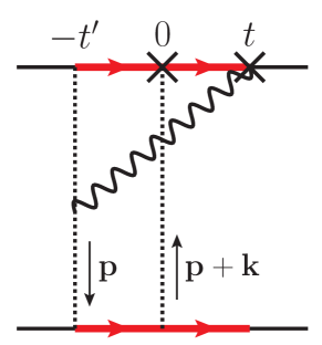
Figure 4: Sample diagram ($3d$) contributing to $\delta E^{(2,0)}_{US}$ and $\delta E^{(1,0)}_{US}$, with time labels on the upper Wilson line vertices and indicated potential three-momentum flow. The thick red lines mark the time interval, where the static quark pair is in a color octet state.

The way we implement the resummation of potential gluon interactions, which actually generates the ultrasoft scale, in our diagrammatic calculation is probably best explained at a concrete example. Let us consider diagram ($3d$) in Figure 1. In Figure 4 we have depicted it with time labels for the vertices on the upper Wilson line and indicated a possible choice for the potential three-momentum flow. The momentum ${\mathbf{k}}$ is the Fourier conjugate to the distance ${\mathbf{r}}$. After expansion and integration over the energies associated with the potential propagators the two vertices on the lower Wilson line are fixed at times $-t^{\prime}$ and $0$, respectively. We have highlighted the time interval, where the static quark-antiquark system is in a color octet state, because the ultrasoft gluon has been radiated off, by thick red static quark (Wilson) lines. During this time interval it is crucial to take into account the exchange of an infinite number of potential Coulomb gluons, between the two Wilson lines. The resummation of such Coulomb interactions yields the LO expression for the average of a rectangular Wilson loop with extensions $t_{2}-t_{1}\gg r$ in the color octet configuration, see e.g. Ref. Brambilla:1999xf :

$$=\theta(t_{2}\!-\!t_{1})\,e^{-iV_{o}^{(0)}(t_{2}-t_{1})}.$$ (23)

The analogous expression with the octet static potential $V_{o}^{(0)}(r)$ replaced by the singlet static potential $V^{(0)}(r)$ holds for the color singlet configuration. Outside the red marked time interval in Figure 4 this exponential however exactly cancels with the singlet Wilson loop average in the denominator of $\langle\langle{\bf E}_{1}^{i}(t){\bf E}_{1}^{j}(0)\rangle\rangle$, whereas inside the octet time interval we can assign a resummed ‘propagator’, $\theta(t_{2}-t_{1})\exp[-i\Delta V(t_{2}-t_{1})]$, to the static quark pair.

In Feynman gauge we thus have

$$\lim_{T\rightarrow\infty}\int_{0}^{T}\mathrm{d}t\;g_{B}^{2}\;t^{n}\;\langle\langle{\bf E}_{1}^{i}(t){\bf E}_{1}^{j}(0)\rangle\rangle\big{|}^{3d}_{\rm US}$$

$$=2\,g_{B}^{6}\bigg{(}\frac{C_{A}^{2}C_{F}}{2}-C_{A}C_{F}^{2}\bigg{)}\int\!\!\frac{\mathrm{d}^{D}q}{(2\pi)^{D}}\int\!\!\frac{\mathrm{d}^{d}p}{(2\pi)^{d}}\int\!\!\frac{\mathrm{d}^{d}k}{(2\pi)^{d}}$$

$$\quad\times e^{-i{\mathbf{k}}{\mathbf{r}}}\;\frac{q_{0}}{q^{2}}\,\frac{p^{i}(p^{j}+k^{j})}{{\mathbf{p}}^{2}({\mathbf{p}}+{\mathbf{k}})^{4}}\;\bigg{(}\int_{0}^{\infty}\!\!\mathrm{d}t^{\prime}\;e^{-i(q_{0}+\Delta V)t^{\prime}}\bigg{)}$$

$$\quad\times\bigg{(}\int_{0}^{\infty}\!\!\mathrm{d}t\;t^{n}\;e^{-i(q_{0}+\Delta V)t}\bigg{)}$$ (24)

$$=-2\,g_{B}^{6}\bigg{(}\frac{C_{A}^{2}C_{F}}{2}-C_{A}C_{F}^{2}\bigg{)}\,\int\!\!\frac{\mathrm{d}^{d}p}{(2\pi)^{d}}\,\frac{p^{i}}{{\mathbf{p}}^{2}}\,e^{-i{\mathbf{p}}{\mathbf{r}}}$$

$$\quad\times\int\!\!\frac{\mathrm{d}^{d}k}{(2\pi)^{d}}\,\frac{k^{j}}{{\mathbf{k}}^{4}}\,e^{-i{\mathbf{k}}{\mathbf{r}}}\int\!\!\frac{\mathrm{d}^{D}q}{(2\pi)^{D}}\;\frac{q_{0}}{q^{2}}\bigg{(}\frac{i}{-q_{0}-\Delta V+i0}\bigg{)}\,$$

$$\quad\times\Bigg{[}\Gamma(1+n)\bigg{(}\frac{i}{-q_{0}-\Delta V+i0}\bigg{)}^{1+n}\Bigg{]}$$ (25)

$$=-g_{B}^{6}\bigg{(}\frac{C_{A}^{2}C_{F}}{2}-C_{A}C_{F}^{2}\bigg{)}\,2^{4-2D}\pi^{1-\frac{3D}{2}}\,\frac{(-i)^{n+1}}{n+1}$$

$$\quad\times\,r^{i}r^{j}\,r^{4-2D}\Delta V^{D-n-3}\,\sin\bigg{(}\frac{\pi D}{2}\bigg{)}$$

$$\quad\times\Gamma\bigg{(}3-\frac{D}{2}\bigg{)}\Gamma(D-4)\Gamma(D-1)\Gamma(3+n-D)\,,$$ (26)

where $D=d+1=4+2\epsilon$, $q$ denotes the ultrasoft four-momentum, $g_{B}$ is the bare version of the coupling, and we have multiplied by $2$ to add the left-right mirror graph exploiting time reversal symmetry. We only kept the leading order in the ultrasoft momentum expansion. Higher orders would come with higher powers of $\alpha$ and are beyond the order we are interested in. For the same reason, we only need the LO expression

$$\Delta V=\frac{g_{B}^{2}}{8}C_{A}\pi^{\frac{1}{2}-\frac{D}{2}}r^{3-D}\Gamma\left(\frac{D-3}{2}\right)+{\mathcal{O}}(g_{B}^{4})$$ (27)

in $D$ dimensions and we can replace the bare coupling $g_{B}$ by the renormalized $g$ as $g_{B}=g+{\cal O}(g^{3})$.

A few practical comments on this example are in order: After performing the last two time integrations we have written Eq. (25) in a suggestive form in terms of momentum space building blocks. The analogous form can be directly obtained for all diagrams in Figures 1 and 2 by assigning the expression in square brackets to the momentum space quark-pair ‘propagator’ between the two crossed vertices and $i/(-q_{0}-\Delta V)$ to the other quark-pair ‘propagators’ between an uncrossed and a crossed vertex, and using momentum space Feynman rules for the vertices and gluon propagators otherwise.

In Coulomb gauge all diagrams with an $A^{0}$ ultrasoft gluon vanish, because the ${\mathbf{q}}$ integral is scaleless after the ultrasoft momentum expansion. To change from Feynman to Coulomb gauge in the diagrams with an ${\mathbf{A}}$ ultrasoft gluon we only have to replace $\delta^{ij}\to\delta^{ij}-q^{i}q^{j}/{\mathbf{q}}^{2}$ in the numerator of the ${\mathbf{A}}$ gluon propagator. It is easy to see that, due to the ultrasoft momentum expansion, this will result in nothing more than an additional overall factor $(D-2)/(D-1)$ for the Coulomb gauge diagrams. In other words, due to gauge invariance, the sum of all diagrams with an ultrasoft $A^{0}$ gluon must be equal to $1/(D-2)$ times the sum of all diagrams with an ultrasoft ${\mathbf{A}}$ gluon. Note that in order to check this explicitly, it is crucial to use the $D$-dimensional expression for $\Delta V$ in Eq. (27).

Also, from our calculation in Eqs. (25) and (26) and the Feynman rules in Figure 3 it should be clear that the diagrams ($3d$) in Figures 1 and 2 yield exactly the same result and in fact all diagrams in Figure 1 equal their counterpart in Figure 2. As we will see below this is related to Poincaré invariance. We therefore conveniently define the quantity

$${\cal W}_{n}^{ij} =\lim_{T\rightarrow\infty}\int_{0}^{T}dt\;t^{n}\,\langle\langle g{\bf E}_{1}^{i}(t)g{\bf E}_{1}^{j}(0)\rangle\rangle_{c}\big{|}_{\rm US}$$

$$=\lim_{T\rightarrow\infty}\int_{0}^{T}dt\,t^{n}\,\langle\langle g{\bf E}_{1}^{i}(t)g{\bf E}_{2}^{j}(0)\rangle\rangle_{c}\big{|}_{\rm US}\;.$$ (28)

with $n=1,2$ for the $1/m$ and $1/m^{2}$ quasi-static energies, respectively. We can then write the ultrasoft contributions to the SI quasi-static energies in Eqs. (15)-(2) as

$$\delta E_{\rm US}^{(1,0)}(r) =-\frac{1}{2}\,\delta^{ij}\,{\cal W}_{1}^{ij}\,,$$ (29)

$$\delta E_{{\mathbf{p}}^{2},\rm US}^{(2,0)}(r) =\frac{i}{2}\,{\hat{\mathbf{r}}^{i}}{\hat{\mathbf{r}}^{j}}\,{\cal W}_{2}^{ij}\,,$$ (30)

$$\delta E_{{\mathbf{L}}^{2},\rm US}^{(2,0)}(r) =\frac{i}{2(d-1)}\left(\delta^{ij}-d\,{\hat{\mathbf{r}}^{i}}{\hat{\mathbf{r}}^{j}}\right){\cal W}_{2}^{ij}\,,$$ (31)

$$\delta E_{{\mathbf{p}}^{2},\rm US}^{(1,1)}(r) =i\,{\hat{\mathbf{r}}^{i}}{\hat{\mathbf{r}}^{j}}\,{\cal W}_{2}^{ij}\,,$$ (32)

$$\delta E_{{\mathbf{L}}^{2},\rm US}^{(1,1)}(r) =\frac{i}{d-1}\left(\delta^{ij}-d\,{\hat{\mathbf{r}}^{i}}{\hat{\mathbf{r}}^{j}}\right){\cal W}_{2}^{ij}\,.$$ (33)

From these equations we can directly read off

$$\delta E_{{\mathbf{L}}^{2},\rm US}^{(1,1)}(r) =2\,\delta E_{{\mathbf{L}}^{2},\rm US}^{(2,0)}(r)\,,$$ (34)

$$\delta E_{{\mathbf{p}}^{2},\rm US}^{(1,1)}(r) =2\,\delta E_{{\mathbf{p}}^{2},\rm US}^{(2,0)}(r)\,.$$ (35)

This verifies Poincaré invariance, see Ref. Barchielli:1988zp . It requires that, given that there is no ultrasoft contribution at ${\mathcal{O}}(\alpha^{2}/m^{0})$, the ${\mathcal{O}}(\alpha^{2}/m^{2})$ ultrasoft part of the total energy of the quark-antiquark system must be proportional to $1/m_{r}^{2}=1/m_{1}^{2}+1/m_{2}^{2}+2/(m_{1}m_{2})$. The corresponding relations for the soft potentials at the same order were checked in Ref. Peset:2015vvi .

From the sum of all relevant ultrasoft one-loop diagrams we obtain the total bare result

$${\cal W}_{n}^{ij}=-\frac{i^{1-n}}{2}\,g_{B}^{2}\,C_{F}\,(D-2)\,\pi^{-D/2}\;\;$$

$$\quad\Gamma\bigg{(}\frac{D}{2}\bigg{)}\,\Delta V^{D-n-1}\Gamma(n+1-D)\Bigg{(}\delta^{ij}$$

$$\quad+\hat{\mathbf{r}}^{i}\hat{\mathbf{r}}^{j}\;\frac{(D-3)(D-n-1)\big{(}D^{2}-D(n+5)+n+2\big{)}}{(n+1)(n+2)}\Bigg{)}\,,$$ (36)

in both Coulomb and Feynman gauge with $\Delta V$ as given in Eq. (27). We emphasize that the connected diagrams in Figure 1 or Figure 2 are not the only diagrams contributing to Eq. (36). In our definition a ‘connected’ graph cannot be split into two (lower loop) Wilson loop diagrams by cutting the quark and the antiquark line at the same time, i.e. by a vertical cut through the diagram. We also have to take into account disconnected (2-Wilson-line reducible) one-loop diagrams as well as (products of) tree-level diagrams from the $\langle\langle{\mathbf{E}}_{a}^{i}(t)\rangle\rangle\langle\langle{\mathbf{E}}_{b}^{j}(0)\rangle\rangle$ term in the definition of the connected Wilson loop average, Eq. (11). Their net effect is however only to remove the terms proportional to $C_{F}^{2}$ and $C_{F}^{3}$ from the connected diagram contributions as explained in detail in the next section. Keeping this in mind it is straightforward to check that the diagrams given in Figures 1 and 2 give the complete $C_{F}$ contribution we are interested in: Every additional diagram with one ultrasoft gluon exchange you can draw, is either disconnected or redundant, in the sense that it is one of the diagrams with additional Coulomb interactions, which we automatically take into account by our resummation. The individual contributions ($\propto C_{F}$) to ${\cal W}_{n}^{ij}$ from each diagram in Figures 1 and 2 are given in Appendix A in Coulomb and Feynman gauge respectively.

We can now use Eq. (36) together with the LO expression Eq. (27) for $\Delta V$ in the ultrasoft contributions Eqs. (29)-(32) and add the bare results for the corresponding potentials in Ref. Peset:2015vvi to obtain finite expressions for the quasi-static energies. With the bare coupling

$$g_{B}^{2}=g^{2}\left(1+\frac{g^{2}\nu^{2\epsilon}}{4\pi}\left(\frac{e^{\gamma_{E}}}{4\pi}\right)^{\epsilon}\frac{\beta_{0}}{4\pi}\frac{1}{\epsilon}\right)$$ (37)

expressed in terms of the $\overline{\rm MS}$ renormalized coupling $\alpha\equiv\alpha(\nu)\equiv\frac{g^{2}\nu^{2\epsilon}}{4\pi}$, we find

$$E^{(1,0)}(r) =V^{(1,0)}(r)+\delta E_{\rm US}^{(1,0)}(r)=$$ (38)

$$-\frac{\alpha^{2}C_{A}C_{F}}{4r^{2}}\bigg{\{}1+\frac{\alpha}{2\pi}\bigg{[}\frac{8}{3}C_{A}\ln(C_{A}\alpha e^{\gamma_{E}})+\frac{47}{18}C_{A}$$

$$-\frac{49}{18}T_{f}n_{f}+2\beta_{0}\ln(e^{\gamma_{E}}\nu r)\bigg{]}\bigg{\}},$$

$$E_{{\bf p}^{2}}^{(2,0)}(r) =V_{{\bf p}^{2}}^{(2,0)}(r)+\delta E_{{\bf p}^{2},\,\rm US}^{(2,0)}(r)=$$

$$-\frac{\alpha^{2}C_{A}C_{F}}{3\pi r}\bigg{\{}\ln(C_{A}\alpha e^{\gamma_{E}})+\frac{1}{4}\bigg{\}},$$ (39)

$$E_{{\bf L}^{2}}^{(2,0)}(r) =V_{{\bf L}^{2}}^{(2,0)}(r)+\delta E_{{\bf L}^{2},\,\rm US}^{(2,0)}(r)=$$

$$-\frac{\alpha^{2}C_{A}C_{F}}{3\pi r}\bigg{\{}2\ln(C_{A}\alpha e^{\gamma_{E}})-1\bigg{\}},$$ (40)

$$E_{{\bf p}^{2}}^{(1,1)}(r) =V_{{\bf p}^{2}}^{(1,1)}(r)+\delta E_{{\bf p}^{2},\,\rm US}^{(1,1)}(r)=$$

$$-\frac{\alpha C_{F}}{r}\bigg{\{}1+\frac{\alpha}{3\pi}\bigg{[}C_{A}\bigg{(}2\ln(C_{A}\alpha e^{\gamma_{E}})-\frac{3}{2}\bigg{)}$$

$$+\beta_{0}\bigg{(}\frac{3}{2}\ln(e^{\gamma_{E}}\nu r)+\frac{1}{2}\bigg{)}\bigg{]}\bigg{\}},$$ (41)

$$E_{{\bf L}^{2}}^{(1,1)}(r) =V_{{\bf L}^{2}}^{(1,1)}(r)+\delta E_{{\bf L}^{2},\,\rm US}^{(1,1)}(r)=$$

$$\frac{\alpha C_{F}}{2r}\bigg{\{}1-\frac{\alpha}{3\pi}\bigg{[}2C_{A}\bigg{(}4\ln(C_{A}\alpha e^{\gamma_{E}})-1\bigg{)}$$

$$+\beta_{0}\bigg{(}\frac{1}{4}-\frac{3}{2}\ln(e^{\gamma_{E}}\nu r)\bigg{)}\bigg{]}\bigg{\}},$$ (42)

after setting $\epsilon\to 0$.

2.2 Cancellation of $C_{F}^{2}$ and $C_{F}^{3}$ terms

As already mentioned in the previous section, the Feynman diagrams we depict in Figure 1 and Figure 2 are the connected (2-Wilson-line irreducible) diagrams relevant for our ultrasoft calculation. It is clear that most of these diagrams are accompanied by a number of disconnected diagrams, which differ from the connected diagrams only by the order of the vertices on the quark lines. For each connected diagram in Figure 1 and Figure 2, let us define a diagram ‘family’, which also includes its disconnected relatives.

Regarding the associated color factor, within each family the connected diagram contains a maximally non-Abelian term, i.e. a term that is linear in the fundamental Casimir constant $C_{F}$. The color factor of the disconnected diagrams consists of terms with at least two powers of $C_{F}$. Summing all diagrams of a family and subtracting the corresponding $\langle\langle{\mathbf{E}}_{a}^{i}(t)\rangle\rangle\langle\langle{\mathbf{E}}_{b}^{j}(0)\rangle\rangle$ term in the definition of the quasi-static energies according to Eq. (11) and Eq. (28), all terms $\propto C_{F}^{n}$ with $n\geq 2$ cancel out and only the maximally non-Abelian term survives. This mechanism is very much reminiscent of the well-known non-Abelian exponentiation Gatheral:1983cz ; Frenkel:1984pz ; Schroder:1999sg of the static potential. For the case of the quasi-static potentials/energies we are lacking however a general proof. We have therefore checked the cancellation of the $C_{F}^{2}$ and $C_{F}^{3}$ terms present in the diagrams with one ultrasoft loop explicitly for each family. In the following we will explain how this works for two diagram families, whose connected graphs are displayed in Figure 1. From this it should be clear how to show the cancellation also for the other families. In particular, all statements in this section can be straightforwardly extended and are therefore equally valid also for the diagrams in Figure 2, which contribute to $\delta E^{(1,1)}_{US}$.

Let us first introduce the notion of a color-stripped diagram. We write e.g.

$$\text{Figure~{}\ref{Vx0Diags}}\;(2c)\;=\;\left(C_{F}^{2}-\frac{C_{A}C_{F}}{2}\right)\raisebox{-11.38109pt}{\includegraphics[height=25.29604pt]{diagrams/CS2c.pdf}}\,.$$ (43)

The graph on the RHS symbolizes the original Feynman diagram with removed (fundamental, anti-fundamental or adjoint) color generators. The red zigzag line represents the ultrasoft gluon.

On the level of such color-stripped diagrams we have

$$\raisebox{-11.38109pt}{\includegraphics[height=25.29604pt]{diagrams/CS2c_1.pdf}}+\raisebox{-11.38109pt}{\includegraphics[height=25.29604pt]{diagrams/CS2c.pdf}}=\raisebox{-11.38109pt}{\includegraphics[height=25.29604pt]{diagrams/CS2c_sing1.pdf}}\times\raisebox{-11.38109pt}{\includegraphics[height=25.29604pt]{diagrams/CS2c_sing2.pdf}}\,.$$ (44)

This can be seen easily as follows. The only difference between the two graphs on the LHS is the lower quark propagator. Labeling the vertex of the ultrasoft gluon with the lower quark line by the time $t^{\prime}$ this propagator is $\theta(t^{\prime}<t)$ and $\theta(t^{\prime}>t)$ in the two diagrams, respectively. After Coulomb resummation some of the $\theta$-functions actually come from the octet bound state propagators and all diagrams with an ultrasoft gluon have a factor $\exp(-i\Delta V|t^{\prime}-t^{\prime\prime}|)$ in common, where in this case $t^{\prime\prime}=0$. For the purpose of this section we can however effectively assign a $\theta$-function to each static quark line in the color-stripped graphs. In the sum of the two one-loop diagrams the $\theta$-functions drop out. As we assume $t>0$ by definition, the upper ‘quark propagator’ $\theta(t>0)$ can also be dropped. Furthermore, by shifting the potential three-momentum ${\mathbf{k}}$ we have (with $q$ being the ultrasoft four-momentum, $d=D-1$)

$$\int\!\!\mathrm{d}^{d}q\int\!\!\mathrm{d}^{d}k\;\frac{e^{i{\mathbf{k}}{\mathbf{r}}}q^{i}(q^{j}+k^{j})}{q^{2}\,({\mathbf{k}}+{\mathbf{q}})^{2}} =$$

$$\int\!\!\mathrm{d}^{d}q\;\frac{q^{i}}{q^{2}}\,e^{-i{\mathbf{q}}{\mathbf{r}}}\times\int\!\!\mathrm{d}^{d}k\;\frac{k^{j}}{{\mathbf{k}}^{2}}\,e^{i{\mathbf{k}}{\mathbf{r}}}$$ (45)

in the integrand of the two one-loop diagrams. Thus we are left with the product of the two tree-level diagrams on the RHS, which will eventually cancel with the corresponding term from $\langle\langle{\mathbf{E}}_{a}^{i}(t)\rangle\rangle\langle\langle{\mathbf{E}}_{b}^{j}(0)\rangle\rangle$). Note that in this case the LO in the ultrasoft momentum expansion ($|{\mathbf{q}}|\ll|{\mathbf{k}}|\sim 1/r$) vanishes due to the antisymmetric ${\mathbf{q}}$-integrand. The NLO in this expansion is nonzero and represents the contribution at the order we are interested in.

With these preliminaries it is straightforward to show the cancellation of the $C_{F}^{2}$ and $C_{F}^{3}$ terms for most of the other diagram families, and we can tackle already the most complicated case, namely the family $3e$. Without the maximally non-Abelian $C_{A}^{2}C_{F}$ term the sum of the diagrams in this family can be written as

$$-C_{F}^{3}\bigg{(}\raisebox{-11.38109pt}{\includegraphics[height=25.29604pt]{diagrams/CS3e_1.pdf}}+\raisebox{-11.38109pt}{\includegraphics[height=25.29604pt]{diagrams/CS3e_2.pdf}}+\raisebox{-11.38109pt}{\includegraphics[height=25.29604pt]{diagrams/CS3e_3.pdf}}\bigg{)}$$

$$+\bigg{(}\frac{C_{A}C_{F}^{2}}{2}-C_{F}^{3}\bigg{)}\bigg{(}\raisebox{-11.38109pt}{\includegraphics[height=25.29604pt]{diagrams/CS3e_4.pdf}}+\raisebox{-11.38109pt}{\includegraphics[height=25.29604pt]{diagrams/CS3e_5.pdf}}$$

$$+\raisebox{-11.38109pt}{\includegraphics[height=25.29604pt]{diagrams/CS3e_6.pdf}}+\raisebox{-11.38109pt}{\includegraphics[height=25.29604pt]{diagrams/CS3e_7.pdf}}\bigg{)}$$

$$+\big{(}C_{A}C_{F}^{2}-C_{F}^{3}\big{)}\bigg{(}\raisebox{-11.38109pt}{\includegraphics[height=25.29604pt]{diagrams/CS3e_8.pdf}}+\raisebox{-11.38109pt}{\includegraphics[height=25.29604pt]{diagrams/CS3e_9.pdf}}\bigg{)}$$ (46)

$$= -C_{F}^{3}\bigg{(}\raisebox{-11.38109pt}{\includegraphics[height=25.29604pt]{diagrams/CS3e_1.pdf}}+\raisebox{-11.38109pt}{\includegraphics[height=25.29604pt]{diagrams/CS3e_2.pdf}}+\raisebox{-11.38109pt}{\includegraphics[height=25.29604pt]{diagrams/CS3e_3.pdf}}$$

$$+\raisebox{-11.38109pt}{\includegraphics[height=25.29604pt]{diagrams/CS3e_4.pdf}}+\raisebox{-11.38109pt}{\includegraphics[height=25.29604pt]{diagrams/CS3e_5.pdf}}+\raisebox{-11.38109pt}{\includegraphics[height=25.29604pt]{diagrams/CS3e_6.pdf}}$$

$$+\raisebox{-11.38109pt}{\includegraphics[height=25.29604pt]{diagrams/CS3e_7.pdf}}+\raisebox{-11.38109pt}{\includegraphics[height=25.29604pt]{diagrams/CS3e_8.pdf}}+\raisebox{-11.38109pt}{\includegraphics[height=25.29604pt]{diagrams/CS3e_9.pdf}}\bigg{)}$$

$$+\frac{C_{A}C_{F}^{2}}{2}\bigg{(}\raisebox{-11.38109pt}{\includegraphics[height=25.29604pt]{diagrams/CSsingcross_1.pdf}}\!\!\times\!\!\raisebox{-11.38109pt}{\includegraphics[height=25.29604pt]{diagrams/CSsingno.pdf}}+\raisebox{-11.38109pt}{\includegraphics[height=25.29604pt]{diagrams/CSsingcross_2.pdf}}\!\!\times\!\!\raisebox{-11.38109pt}{\includegraphics[height=25.29604pt]{diagrams/CSsingno.pdf}}$$

$$+\raisebox{-11.38109pt}{\includegraphics[height=25.29604pt]{diagrams/CSsingno.pdf}}\!\!\times\!\!\raisebox{-11.38109pt}{\includegraphics[height=25.29604pt]{diagrams/CSsingcross_1.pdf}}+\raisebox{-11.38109pt}{\includegraphics[height=25.29604pt]{diagrams/CSsingno.pdf}}\!\!\times\!\!\raisebox{-11.38109pt}{\includegraphics[height=25.29604pt]{diagrams/CSsingcross_2.pdf}}\bigg{)}\,.$$ (47)

Exploiting again the static quark line $\theta$-functions, we have used the equalities

$$\raisebox{-11.38109pt}{\includegraphics[height=25.29604pt]{diagrams/CS3e_4.pdf}}+\raisebox{-11.38109pt}{\includegraphics[height=25.29604pt]{diagrams/CS3e_8.pdf}} =\raisebox{-11.38109pt}{\includegraphics[height=25.29604pt]{diagrams/CSsingcross_1.pdf}}\!\!\times\!\!\raisebox{-11.38109pt}{\includegraphics[height=25.29604pt]{diagrams/CSsingno.pdf}}\;,$$ (48)

$$\raisebox{-11.38109pt}{\includegraphics[height=25.29604pt]{diagrams/CS3e_5.pdf}}+\raisebox{-11.38109pt}{\includegraphics[height=25.29604pt]{diagrams/CS3e_8.pdf}} =\raisebox{-11.38109pt}{\includegraphics[height=25.29604pt]{diagrams/CSsingno.pdf}}\!\!\times\!\!\raisebox{-11.38109pt}{\includegraphics[height=25.29604pt]{diagrams/CSsingcross_1.pdf} },$$ (49)

and their analogs for the graphs, where the ultrasoft gluon is up-down mirrored, in Eq. (47) to write the $C_{F}^{2}$ term as a sum of products of one-loop and tree-level diagrams with a single insertion of an ${\mathbf{E}}$-field operator. Recall that in our notation the operator insertion vertex on the left is always located at time $0$ and the one on the right at time $t$ with $t>0$. The two expressions on the RHS of Eq. (48) and Eq. (49) are therefore unequal. The $C_{F}^{2}$ term of Eq. (47) will be directly cancelled by the corresponding $C_{F}^{2}$ term from the $\langle\langle{\mathbf{E}}_{1}^{i}(t)\rangle\rangle\langle\langle{\mathbf{E}}_{1}^{j}(0)\rangle\rangle$ part of the definition of the quasi-static energies.

The cancellation of the $C_{F}^{3}$ term is a bit more subtle. First we note that

$$\raisebox{-11.38109pt}{\includegraphics[height=25.29604pt]{diagrams/CS3e_3.pdf}}+\raisebox{-11.38109pt}{\includegraphics[height=25.29604pt]{diagrams/CS3e_6.pdf}}+\raisebox{-11.38109pt}{\includegraphics[height=25.29604pt]{diagrams/CS3e_1.pdf}}$$

$$+\raisebox{-11.38109pt}{\includegraphics[height=25.29604pt]{diagrams/CS3e_4.pdf}}=\raisebox{-11.38109pt}{\includegraphics[height=25.29604pt]{diagrams/CSsingno.pdf}}\!\!\times\!\!\raisebox{-11.38109pt}{\includegraphics[height=25.29604pt]{diagrams/CSsingparallel_1.pdf} }\,,$$ (50)

by combining the $\theta$-functions from the upper and lower static quark lines. Also, (after shifting a potential three-momentum) we directly have

$$\raisebox{-11.38109pt}{\includegraphics[height=25.29604pt]{diagrams/CS3e_1.pdf}}=\raisebox{-11.38109pt}{\includegraphics[height=25.29604pt]{diagrams/CSsingparallel_1.pdf}}\!\!\times\!\!\raisebox{-11.38109pt}{\includegraphics[height=25.29604pt]{diagrams/CSsingno.pdf} }\,.$$ (51)

With the equalities in Eqs. (48)-(51) and their analogs for the mirror graphs we can write the $C_{F}^{3}$ term of Eq. (47) in factorized form:

$$-\frac{C_{F}^{3}}{2}\Bigg{[}\bigg{(}\raisebox{-11.38109pt}{\includegraphics[height=25.29604pt]{diagrams/CSsingparallel_1.pdf}}+\raisebox{-11.38109pt}{\includegraphics[height=25.29604pt]{diagrams/CSsingcross_1.pdf}}+\raisebox{-11.38109pt}{\includegraphics[height=25.29604pt]{diagrams/CSsingparallel_2.pdf}}$$

$$\qquad+\raisebox{-11.38109pt}{\includegraphics[height=25.29604pt]{diagrams/CSsingcross_2.pdf}}\bigg{)}\times\!\!\raisebox{-11.38109pt}{\includegraphics[height=25.29604pt]{diagrams/CSsingno.pdf} }+\!\!\raisebox{-11.38109pt}{\includegraphics[height=25.29604pt]{diagrams/CSsingno.pdf}}\!\!\times\bigg{(}\raisebox{-11.38109pt}{\includegraphics[height=25.29604pt]{diagrams/CSsingparallel_1.pdf}}$$

$$\qquad+\raisebox{-11.38109pt}{\includegraphics[height=25.29604pt]{diagrams/CSsingcross_1.pdf}}+\raisebox{-11.38109pt}{\includegraphics[height=25.29604pt]{diagrams/CSsingparallel_2.pdf}}+\raisebox{-11.38109pt}{\includegraphics[height=25.29604pt]{diagrams/CSsingcross_2.pdf}}\bigg{)}\Bigg{]}\,.$$ (52)

Apart from the overall factor $1/2$ this is what one might naively expect for the $C_{F}^{3}$ term from $\langle\langle{\mathbf{E}}_{1}^{i}(t)\rangle\rangle\langle\langle{\mathbf{E}}_{1}^{j}(0)\rangle\rangle$ at NLO in the ultrasoft loop expansion. On the first sight there therefore seems to be miscancellation of the $C_{F}^{3}$ terms. Let us however take a closer look at Eq. (52). Similar to Eq. (50) the expressions in round brackets can be factorized further and we are left with

$$-C_{F}^{3}\raisebox{-11.38109pt}{\includegraphics[height=25.29604pt]{diagrams/CSsingno.pdf}}\!\!\times\!\!\raisebox{-11.38109pt}{\includegraphics[height=25.29604pt]{diagrams/CSsingno.pdf}}\!\!\times\!\!\raisebox{-11.38109pt}{\includegraphics[height=25.29604pt]{diagrams/CSsingUS.pdf}}\,.$$ (53)

Now, recall that in the definition of $\langle\langle{\mathbf{E}}_{1}(t){\mathbf{E}}_{1}(0)\rangle\rangle$ there is the singlet Wilson loop average in the denominator. At LO we simply have $\langle W_{\Box}\rangle$ = $\exp(-iV_{s}T_{W})$, but at the NLO in the ultrasoft loop expansion we obtain

$$C_{F}^{3}\raisebox{-11.38109pt}{\includegraphics[height=25.29604pt]{diagrams/CSdoubleno.pdf}}\!\!\times\!\!\raisebox{-11.38109pt}{\includegraphics[height=25.29604pt]{diagrams/CSsingUS.pdf}}=C_{F}^{3}\raisebox{-11.38109pt}{\includegraphics[height=25.29604pt]{diagrams/CSsingno.pdf}}\!\!\times\!\!\raisebox{-11.38109pt}{\includegraphics[height=25.29604pt]{diagrams/CSsingno.pdf}}\!\!\times\!\!\raisebox{-11.38109pt}{\includegraphics[height=25.29604pt]{diagrams/CSsingUS.pdf}}$$ (54)

as an additional contribution to the quasi-static energies. Thus the total $C_{F}^{3}$ term from the $\langle\langle{\mathbf{E}}_{1}^{i}(t){\mathbf{E}}_{1}^{j}(0)\rangle\rangle$ vanishes. It is easy to see that the same happens separately for the $C_{F}^{3}$ term associated with $\langle\langle{\mathbf{E}}_{1}^{i}(t)\rangle\rangle\langle\langle{\mathbf{E}}_{1}^{j}(0)\rangle\rangle$. There we have two times Eq. (53) plus two times the RHS of Eq. (54) from the expansion of the two denominators in $\langle\langle{\mathbf{E}}_{1}^{i}(t)\rangle\rangle\langle\langle{\mathbf{E}}_{1}^{j}(0)\rangle\rangle$. This completes the proof of the cancellation of the $C_{F}^{2}$ and $C_{F}^{3}$ terms related to family $3e$.

Analogous proofs hold for families $3f$ and $3g$. Adding the contributions to ${\cal W}_{n}^{ij}$ from diagram families $3e$, $3f$ and $3g$ the LO terms in the ultrasoft momentum expansion, i.e. terms $\sim\alpha^{3}\Delta V^{-1-n}r^{-4}$, cancel out, but a contribution $\sim\alpha^{3}\Delta V^{1-n}r^{-2}\sim\alpha^{4-n}r^{n-3}$, which is the order of our interest, survives. We note that the diagram families ($2c$, $3e$, $3f$, $3g$) discussed above actually vanish in Coulomb gauge.

For the families with an ultrasoft ${\mathbf{A}}$ gluon ($3d$, $4a$, $4b$, $5a$) relevant also in Coulomb gauge the proofs are, in fact, even simpler than the ones presented here and straightforward to do with the above techniques. We have thus shown ‘non-Abelian exponentiation’ of the $1/m$ and $1/m^{2}$ quasi-static energies at one ultrasoft loop.

3 Resummation of large logs

Our finite order results for the quasi-static energies in Eqs. (38)-(2.1) depend on the factorization/renormalization scale $\nu$. Setting $\nu\sim 1/r$ large logarithms associated with the soft scale are resummed in the running coupling $\alpha(\nu)$. For the complete resummation of large logarithms, also ultrasoft logarithms have to be resummed. In this section we discuss how this can be achieved.

The bare potential (in the Wilson loop scheme) can be written in terms of the renormalized potential and its counterterm as

$$V_{s,B}=V_{s}+\delta V_{s}\,.$$ (55)

The counterterm $\delta V_{s}$ for the potentials in terms of Wilson loops can be determined at leading order from the (IR) $1/\epsilon$ terms of the soft contribution computed in Ref. Peset:2015vvi . It can also be obtained (at leading order) from our ultrasoft calculation in the present paper. Indeed the $1/\epsilon$ terms of both computations match, which guarantees that we obtain finite results in Eqs. (38)-(2.1). At leading order the structure of the counterterm is (cf. Eq. (58) below)

$$\delta V\sim\frac{1}{\epsilon}\alpha^{n}\times F({\bf r}^{2})\,,$$ (56)

where $n$ and $F$ depend on the specific potential $V$. This information by itself is not enough to obtain the leading-log (LL) running for each potential in the Wilson loop scheme. Still, this problem can be bypassed at LL, since EFT arguments tell us that the structure of the LO overall counterterm should be (note that $\nu$ here refers to $\nu_{us}$)

$$\delta V_{s}\sim\frac{1}{\epsilon}\alpha(\nu)V_{A}^{2}\times G(V^{(0)};V_{o}^{(0)}),$$ (57)

where $G$ is a function of the singlet/octet static potentials, and $V_{A}=1$ at this order.

Let us now link this discussion to previous determinations of the counterterm $\delta V_{s}$ in the direct context of EFTs. If the counterterm is determined in an EFT calculation in terms of the Wilson coefficients of the EFT it is possible to resum the ultrasoft logarithms into the potentials by solving the associated renormalization group equations (RGEs). Since our derivation of the quasi-static energies is based on the method of regions rather than on an EFT, we have a priori no RGEs at hand to resum such logarithms. Using the EFT, the counterterm and the associated RGE for the next-to-leading-log (NLL) ultrasoft running of $V_{s}$ were obtained in Ref. Pineda:2011aw (the LL ultrasoft running of $V_{s}$ was obtained in Ref. Pineda:2001ra ). These expressions are suitable for the potentials in the on-shell or Feynman/Coulomb gauge off-shell matching schemes. However, as explained in Ref. Peset:2015vvi , the counterterm of Ref. Pineda:2011aw fails to cancel the divergences of the individual potentials in the Wilson loop matching scheme. Therefore we proposed a modified counterterm, that removes the divergences from the individual potentials at LO for that scheme Peset:2015vvi . Such a counterterm directly follows from the computation and the knowledge of the structure of the counterterm in Eq. (57), as we discussed above. We conjecture that the structure of this counterterm is preserved at NLO. Adding the NLO piece according to Ref. Pineda:2011aw gives the following expression for the counterterm in the Wilson loop matching scheme ($W$):

$$\delta V_{s,W}=\Bigg{(}{\bf r}^{2}(\Delta V)^{3}-\frac{1}{2m_{r}^{2}}\left[{\bf p},\left[{\bf p},V^{(0)}_{o}\right]\right]$$

$$\quad+\frac{1}{2m_{r}^{2}}\left\{{\bf p}^{2},\Delta V\right\}+\frac{i}{2m_{r}^{2}}\left\{{\bf p}^{i},\left\{{\bf p}^{j},[{\bf p}^{j},\Delta Vr^{i}]\right\}\right\}$$

$$\quad+\frac{1}{2m_{r}}\Bigg{[}(\Delta V)^{2}(3d-5)+4\Delta V\left(\left(r\frac{d}{dr}\Delta V\right)+\Delta V\right)$$

$$\quad+\left(\left(r\frac{d}{dr}\Delta V\right)+\Delta V\right)^{2}\Bigg{]}\Bigg{)}$$

$$\times\Bigg{[}\frac{1}{\epsilon}C_{F}V_{A}^{2}\bigg{[}\frac{\alpha(\nu)}{3\pi}-\frac{\alpha^{2}(\nu)}{36\pi^{2}}\bigg{(}\frac{10}{3}T_{F}n_{f}-C_{A}\bigg{(}\frac{47}{3}+2\pi^{2}\bigg{)}\bigg{)}\bigg{]}$$

$$\quad+\frac{1}{\epsilon^{2}}C_{F}V_{A}^{2}\frac{2}{3}\beta_{0}\frac{\alpha^{2}(\nu)}{(4\pi)^{2}}\Bigg{]}.$$ (58)

At LO this is correct, because $\delta V_{s,W}$ correctly reproduces the UV divergence of the ultrasoft contribution to all quasi-static energies we have calculated. At NLO and beyond it is only a conjecture, because in our approach we have no proper control on (potential) operator mixing effects in the RGE. We will nevertheless use the resulting expressions as an educated guess for the renormalized NLL potentials $V_{s,W}$. We hope that an EFT analysis will eventually settle this issue.

The RGE then reads

$$\nu\frac{d}{d\nu}V_{s,\overline{\rm MS}}=B_{V_{s}}\,,$$ (59)

where

$$B_{V_{s}} =C_{F}\Biggl{(}{\bf r}^{2}(\Delta V)^{3}-\frac{1}{2m_{r}^{2}}\left[{\bf p},\left[{\bf p},V^{(0)}_{o}\right]\right]$$

$$+\frac{1}{2m_{r}^{2}}\left\{{\bf p}^{2},\Delta V\right\}+\frac{i}{2m_{r}^{2}}\left\{{\bf p}^{i},\left\{{\bf p}^{j},[{\bf p}^{j},\Delta Vr^{i}]\right\}\right\}$$

$$+\frac{1}{2m_{r}}\left[4(\Delta V)^{2}+4\Delta V\left(\left(r\frac{d}{dr}\Delta V\right)+\Delta V\right)\right.$$

$$\left.+\left(\left(r\frac{d}{dr}\Delta V\right)+\Delta V\right)^{2}\right]\Biggr{)}\left[-\frac{2\alpha(\nu)}{3\pi}\right.$$

$$\left.+\frac{\alpha^{2}(\nu)}{9\pi^{2}}\bigg{(}\frac{10}{3}T_{F}n_{f}-C_{A}\bigg{(}\frac{47}{3}+2\pi^{2}\bigg{)}\bigg{)}+{\cal O}(\alpha^{3})\right].$$ (60)

Here and in the following the Wilson loop scheme for the potentials is understood and we drop the corresponding subscript $W$ for brevity. We also set the pNRQCD Wilson coefficient $V_{A}=1$, which is consistent at LL Pineda:2000gza and NLL Brambilla:2009bi .

We write the running potential as

$$V_{s,\rm RG}(r;\nu_{us}) =V_{s}(r;\nu)+\delta V_{s,\rm RG}(r;\nu,\nu_{us})\,,$$ (61)

with $\delta V_{s,\rm RG}(r;\nu,\nu_{us}\!=\!\nu)=0$. We now only consider the $1/m$ and the $1/m^{2}$ SI momentum-dependent potentials. Solving the RGEs and truncating at the appropriate order in $\alpha$ we obtain

$$\delta V^{(1,0)}_{\rm RG}(r;\nu,\nu_{us}) =2\left(\frac{C_{A}\alpha(\nu)}{2r}\right)^{2}$$

$$\times\left(1+2\frac{\alpha(\nu)}{4\pi}\left(a_{1}+2\beta_{0}\ln(\nu e^{\gamma_{E}+\frac{1}{2}}r)\right)\right)F(\nu;\nu_{us})\,,$$ (62)

$$\delta V^{(2,0)}_{{\bf p}^{2},\rm RG}(r;\nu,\nu_{us}) =$$

$$\frac{C_{A}\alpha(\nu)}{2r}\left(1+\frac{\alpha(\nu)}{4\pi}\left(a_{1}+2\beta_{0}\ln(\nu e^{\gamma_{E}+2}r)\right)\right)F(\nu;\nu_{us})\,,$$ (63)

$$\delta V^{(2,0)}_{{\bf L}^{2},\rm RG}(r;\nu,\nu_{us}) =$$

$$\frac{C_{A}\alpha(\nu)}{r}\left(1+\frac{\alpha(\nu)}{4\pi}\left(a_{1}+2\beta_{0}\ln(\nu e^{\gamma_{E}-1}r)\right)\right)F(\nu;\nu_{us})\,,$$ (64)

$$\delta V^{(1,1)}_{{\bf p}^{2},\rm RG}(r;\nu,\nu_{us}) =$$

$$\frac{C_{A}\alpha(\nu)}{r}\left(1+\frac{\alpha(\nu)}{4\pi}\left(a_{1}+2\beta_{0}\ln(\nu e^{\gamma_{E}+2}r)\right)\right)F(\nu;\nu_{us})\,,$$ (65)

$$\delta V^{(1,1)}_{{\bf L}^{2},\rm RG}(r;\nu,\nu_{us}) =$$

$$\frac{2C_{A}\alpha(\nu)}{r}\left(1+\frac{\alpha(\nu)}{4\pi}\left(a_{1}+2\beta_{0}\ln(\nu e^{\gamma_{E}-1}r)\right)\right)F(\nu;\nu_{us})\,,$$ (66)

where

$$F(\nu;\nu_{us})=C_{F}\frac{2\pi}{\beta_{0}}\bigg{\{}\frac{2}{3\pi}\ln\frac{\alpha(\nu_{us})}{\alpha(\nu)}-\big{(}\alpha(\nu_{us})-\alpha(\nu)\big{)}$$

$$\times\left(\frac{8}{3}\frac{\beta_{1}}{\beta_{0}}\frac{1}{(4\pi)^{2}}-\frac{1}{27\pi^{2}}\left(C_{A}\left(47+6\pi^{2}\right)-10T_{F}n_{f}\right)\right)\bigg{\}}\,.$$ (67)

We computed the $\overline{\rm MS}$ renormalized (Wilson loop) potentials at $\nu_{us}\!=\!\nu$ in Ref. Peset:2015vvi . For convenience we quote the results here:

$$V^{(1,0)}(r;\nu) =-\frac{C_{F}C_{A}\alpha^{2}(e^{-\gamma_{E}}/r)}{4r^{2}}$$

$$\left\{1+\frac{\alpha}{\pi}\left(\frac{89}{36}C_{A}-\frac{49}{36}T_{F}n_{f}+\frac{4}{3}C_{A}\ln\left(\nu re^{\gamma_{E}}\right)\right)\right\},$$ (68)

$$V^{(2,0)}_{{\bf p}^{2}}(r;\nu) =-\frac{C_{A}C_{F}\alpha^{2}}{\pi r}\left(\frac{2}{3}+\frac{1}{3}\ln\left(r\nu e^{\gamma_{E}}\right)\right),$$ (69)

$$V^{(2,0)}_{{\bf L}^{2}}(r;\nu) =\frac{C_{A}C_{F}\alpha^{2}}{4\pi r}\left(\frac{11}{3}-\frac{8}{3}\ln\left(r\nu e^{\gamma_{E}}\right)\right),$$ (70)

$$V^{(1,1)}_{{\bf p}^{2}}(r;\nu) =-C_{F}\frac{\alpha(e^{-\gamma_{E}}/r)}{r}$$

$$\left\{1+\frac{\alpha}{\pi}\left(\frac{23}{18}C_{A}-\frac{2}{9}T_{F}n_{f}+\frac{2}{3}C_{A}\ln\left(\nu re^{\gamma_{E}}\right)\right)\right\},$$ (71)

$$V^{(1,1)}_{{\bf L}^{2}}(r;\nu) =\frac{C_{F}\alpha(e^{-\gamma_{E}}/r)}{2r}$$

$$\left\{1+\frac{\alpha}{\pi}\left(\frac{97C_{A}}{36}+\frac{1}{9}T_{F}n_{f}-\frac{8}{3}C_{A}\ln\left(\nu re^{\gamma_{E}}\right)\right)\right\}.$$ (72)

Including the resummation of ultrasoft logarithms the total quasi-static energy then reads

$$E_{s,\rm RG}(r) =V_{s,\rm RG}(r;\nu_{us})+\delta E_{{\rm US}}(r;\nu_{us})\,,$$ (73)

and similarly for the individual quasi-static energies we discuss in this paper. The corresponding $\overline{\rm MS}$ renormalized ultrasoft parts are

$$\delta E^{(1,0)}_{\rm US}(r;\nu_{us}) =$$

$$-\frac{\alpha^{2}(\nu)\alpha(\nu_{us})C_{F}C_{A}^{2}}{3\pi r^{2}}\left\{\ln\left(\frac{C_{A}\,\alpha(\nu)}{\nu_{us}r}\right)-\frac{7}{8}\right\},$$ (74)

$$\delta E^{(2,0)}_{{\bf p}^{2},\rm US}(r;\nu_{us}) =$$

$$-\frac{\alpha(\nu)\alpha(\nu_{us})C_{F}C_{A}}{3\pi r}\left\{\ln\left(\frac{C_{A}\,\alpha(\nu)}{\nu_{us}r}\right)-\frac{7}{4}\right\},$$ (75)

$$\delta E^{(2,0)}_{{\bf L}^{2},\rm US}(r;\nu_{us}) =$$

$$-\frac{2\alpha(\nu)\alpha(\nu_{us})C_{F}C_{A}}{3\pi r}\left\{\ln\left(\frac{C_{A}\,\alpha(\nu)}{\nu_{us}r}\right)+\frac{7}{8}\right\},$$ (76)

$$\delta E^{(1,1)}_{{\bf p}^{2},\rm US}(r;\nu_{us}) =$$

$$-\frac{2\alpha(\nu)\alpha(\nu_{us})C_{F}C_{A}}{3\pi r}\left\{\ln\left(\frac{C_{A}\,\alpha(\nu)}{\nu_{us}r}\right)-\frac{7}{4}\right\},$$ (77)

$$\delta E^{(1,1)}_{{\bf L}^{2},\rm US}(r;\nu_{us}) =$$

$$-\frac{4\alpha(\nu)\alpha(\nu_{us})C_{F}C_{A}}{3\pi r}\left\{\ln\left(\frac{C_{A}\,\alpha(\nu)}{\nu_{us}r}\right)+\frac{7}{8}\right\}.$$ (78)

Formally, these ultrasoft contributions are independent of $\nu$, as in pNRQCD the soft scale has already been integrated out. In practice they do depend on $\nu$ once we allow for the running of $\alpha(\nu)$. This however affects the result only beyond the order to which the ultrasoft computation has been carried out. For a meaningful evaluation of the (RG improved) quasi-static energies $\nu\approx 1/r$ and $\nu_{us}\approx C_{A}\alpha/r$ must be chosen.

4 Comparison with lattice data

Monte Carlo lattice simulations of the $1/m$ and $1/m^{2}$ SI momentum-dependent quasi-static energies have been performed over the years Bali:1997am ; Koma:2007jq ; Koma:2009ws . The data for the SI momentum-dependent $1/m^{2}$ contributions is usually displayed in terms of the following linear combinations of the quasi-static energies:

$$E_{b}(r) =-\frac{2}{3}E_{\textbf{L}^{2}}^{(1,1)}(r)-E_{{\bf p}^{2}}^{(1,1)}(r),$$ (79)

$$E_{c}(r) =-E_{\textbf{L}^{2}}^{(1,1)}(r),$$ (80)

$$E_{d}(r) =\frac{2}{3}E_{\textbf{L}^{2}}^{(2,0)}(r)+E_{{\bf p}^{2}}^{(2,0)}(r),$$ (81)

$$E_{e}(r) =E_{\textbf{L}^{2}}^{(2,0)}(r).$$ (82)

Therefore, we will directly confront our results with these quantities in the following section. On the lattice side we will use the most recent results obtained in Refs. Koma:2007jq ; Koma:2009ws , also for the comparison with the $1/m$ quasi-static energy.

4.1 Short distances

Lattice data is very scarce at short distances. It is also worth mentioning that at short distances one can easily see finite discretization effects in the lattice data. On top of that, due to possible power-like divergences in the lattice simulation, we cannot compare with the lattice data in absolute values. We are thus forced to consider differences between quasi-static energies computed at different distances. We then choose to normalize our results to the lattice point at the shortest available distance for each observable. This leaves us with at most three independent lattice points (in fact only two for $E_{b}$ and $E_{c}$) for distances smaller than $0.5\,r_{0}\approx 0.8$ GeV, which is already at the borderline for our weak coupling results to be reliable. Therefore, the whole discussion in this section will stay at the qualitative level.

The analytic results we present in the plots of this section are based on Eqs. (38)-(2.1). For the resummation of the ultrasoft logarithms we will use the the results of Section 3. We will first define the different curves shown in these plots and discuss them in comparison with the available lattice data afterwards. The different colors of the lattice data points in our plots (with hardly visible error bars) indicate different $\beta$ values (blue: $\beta=5.85$, green: $\beta=6$, brown: $\beta=6.2$), see Refs. Koma:2007jq ; Koma:2009ws . For $E^{(1,0)}$, $E_{b}$ and $E_{c}$ Eqs. (38)-(2.1) give the first two (LO and NLO) nontrivial terms, whereas for $E_{d}$ and $E_{e}$ they only yield the first (NLO) nontrivial term in the weak coupling expansion. The scale dependence of the coupling constant is uncancelled beyond NLO. We use this fact to grasp the dependence of our predictions on higher order corrections. On the one hand we produce curves with a fixed, $r$-independent factorization scale $\nu$. For these, we take as a reference scale the shortest distance of the available lattice points, and vary $\nu$ around this value. For $E^{(1,0)}$, $E_{d}$ and $E_{e}$, we take $\nu=x/0.153990\;r_{0}^{-1}$ and for $E_{b}$ and $E_{c}$ we take $\nu=x/0.371627\;r_{0}^{-1}$. Here and in the following the parameter $x$ always represents a number of order $1$. On the other hand we also produce curves with $\nu=x/r$. The obvious motivation of this is to resum logarithms of $\nu r$. This is however not sufficient to resum all large logarithms, as there are also ultrasoft logarithms. In order to perform a complete resummation of logarithms, we have to use Eqs. (61)-(78) and count $\alpha(\nu)\sim\alpha(\nu_{us})$, so that the resummation kernel $F(\nu,\nu_{us})\sim 1$. With this counting the ${\cal O}(\alpha^{2})$ term in the expression for the $1/m$ and the ${\cal O}(\alpha)$ term in the expression for the $1/m^{2}$ quasi-static energies, represents the results with LL accuracy. Our complete expressions for the quasi-static energies according to Eq. (73) represents an educated guess of the NLL expression and we use it as an estimate of the next order. The dependence on $\nu$ and $\nu_{us}$ cancels in the theoretical expression at NLL but not beyond. Again, this residual dependence may give hints on the size of higher order terms. We will generate lines with $\nu=x/r$ and $\nu_{us}=x_{us}C_{A}\alpha_{\rm s}(\nu)/r$, with $x\sim x_{us}\sim 1$. Note that the RG improved expressions reduce to the ‘fixed order’ expressions in Eqs. (38)-(2.1) when fixing $\nu=\nu_{us}$ in Eqs. (61)-(78).

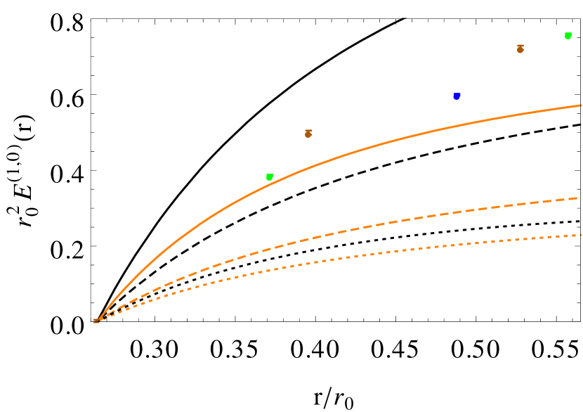
Figure 5: Comparison to the lattice data for $E^{(1,0)}(r)$. The solid lines correspond to the LO (orange) and NLO results (black) at fixed scale $\nu=2\times 1/0.263821$ $r_{0}^{-1}$. The dashed lines correspond to the LO (orange) and NLO (black) setting $\nu=3/r$. The dotted lines correspond to the LL (orange) and NLL results (black) setting $\nu_{us}=2C_{A}\alpha(\nu)/r$ and $\nu=3/r$.

We first consider the $1/m$ quasi-static energy at LO and NLO. We observe that the uncertainties are quite large. This is reflected in a strong scale dependence, which could be expected as we are evaluating our result at very low scales and already the LO is ${\cal O}(\alpha^{2})$. Even using the one-loop or two-loop expression for the running $\alpha$ produces sizable differences. Nevertheless, it is comforting that we can find reasonable values of $\nu$ such that the curves match the lattice data quite well ($\nu\approx 3.4/0.264\;r_{0}^{-1}\approx 5.2$ GeV for the NLO and $\nu\approx 1.6/0.264$ $r_{0}^{-1}\approx 2.4$ GeV for the LO), even though the difference between LO and NLO is relatively large. To illustrate this difference we show curves for the LO and NLO results with fixed $\nu=2\times 1/0.263821$ $r_{0}^{-1}\approx 3$ GeV in Figure 5. We also show the corresponding curves with $\nu=3/r$. They hardly differ from the choice $\nu=2/r$ and lie below the lattice points, but are still consistent with them within the expected uncertainties. The effect of setting $\nu\geq 2/r$ is making the series more convergent: The difference between LO and NLO becomes smaller compared to the fixed scale results as observed in Figure 5. However, $\nu\leq 1/r$ is a too small scale and the perturbation series blows up (which may be due to renormalons). A systematic resummation of all large logarithms requires setting $\nu_{us}\sim C_{A}\alpha(\nu)/r$ and $\nu\sim 1/r$. The additional resummation of ultrasoft logarithms further improves the convergence (LO and NLO curves are closer), but the curves also lie further below the lattice points, see Figure 5. Just like for the ‘fixed order predictions’ with $r$-dependent factorization scale, we have to choose relatively large values of $\nu$ to avoid unphysical behavior.

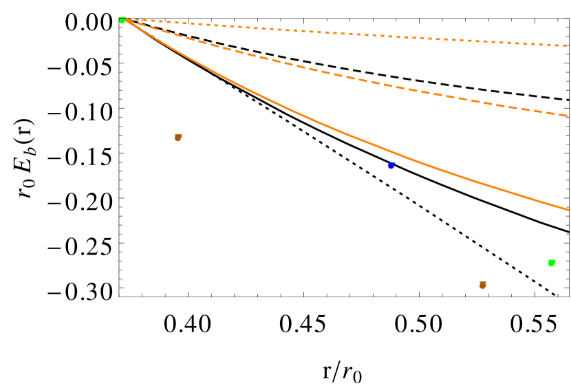
Figure 6: Comparison to the lattice data for $E_{b}$. The solid lines correspond to the LO (orange) and NLO results (black) at fixed scale $\nu=2\times 1/0.371627$ $r_{0}^{-1}$. The dashed lines correspond to the LO (orange) and NLO results (black) setting $\nu=4/r$. The dotted lines correspond to the LL (orange) and NLL results (black) setting $\nu_{us}=C_{A}\alpha(\nu)/r$ and $\nu=4/r$.

Next we consider $E_{b}$. The situation here is far from optimal, as illustrated in Figure 6. We have one less lattice data point (the one at shortest distance) than for $E^{(1,0)}$, which makes the region, where we can compare with the lattice data, even smaller. There are also visible finite size effects in the lattice data, when comparing the points for different values of $\beta$. This indicates that a global negative shift of our lines would be appropriate in the comparison with the lattice data. We do not implement this shift explicitly in Figure 6, but it is understood in the following discussion. With fixed $\nu$ the agreement is reasonable. For $\nu\approx 1.5\times 1/0.371627$ $r^{-1}_{0}$ the NLO result agrees well with the data and so does the LO result, as there are only small differences between the two curves. Choosing $\nu\sim 1/r$ deteriorates the agreement. As for the $1/m$ quasi-static energy, setting $\nu\leq 1/r$ causes the perturbation series to blow up (maybe due to renormalons) as the scale becomes too small. The complete resummation of logarithms yields strongly scale-dependent results. If one takes $\nu_{us}=C_{A}\alpha(\nu)/r$ and $\nu=4/r$ the agreement with the data is very good at NLL but the difference to the LL prediction is very large. Also, we observe a strong dependence of the result on $x_{us}$ (not displayed) in the range between one and two. In any case the uncertainties are large.

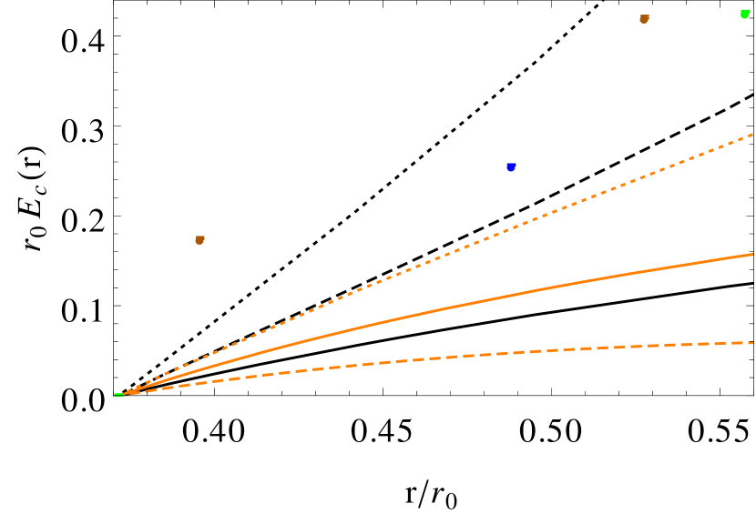
Figure 7: Comparison to the lattice data for $E_{c}$. The solid lines correspond to the LO (orange) and NLO results (black) at fixed scale $\nu=2\times 1/0.371627r_{0}^{-1}$. The dashed lines correspond to the LO (orange) and NLO (black) results setting $\nu=1/r$. The dotted lines correspond to the LL (orange) and NLL (black) results setting $\nu_{us}=C_{A}\alpha(\nu)/r$ and $\nu=1/r$.

For $E_{c}$, the situation is similar as for $E_{b}$ as far as the number and location of the lattice points are concerned, see Figure 7. Note that there are again sizable finite size effects in the lattice data. So, it would be reasonable to add a global shift upwards to all our lines when making the comparison with data. Working at fixed order with fixed scale the slope is smaller than predicted by the data, as can be seen in Figure 7 for $x=2$. Setting $\nu\sim 1/r$ does not help much, until we set $\nu\approx 1/r$, where the NLO result gets quite close to the lattice data (unlike in the previous cases here we can set $\nu$ quite low). However, it still shows a huge difference to the LO result. Similarly, the resummation of ultrasoft logarithms does not improve the situation, unless we choose $x\approx x_{us}\approx 1$, where one can get good agreement with the data. Nevertheless, once more the scale dependence is large.

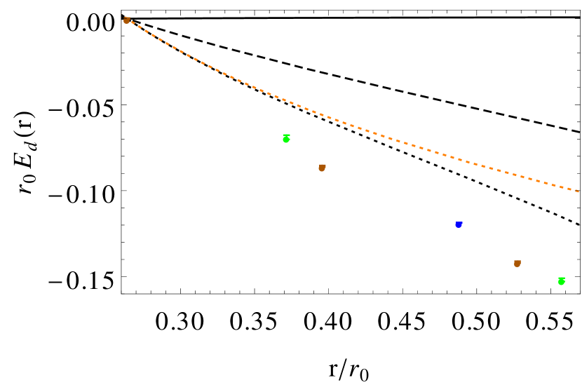
Figure 8: Comparison to the lattice data for $E_{d}$. The solid black line corresponds to the NLO result at fixed scale $\nu=2/0.263821r_{0}^{-1}$. The dashed black line corresponds to the NLO result setting $\nu=2/r$. The dotted lines correspond to the LL (orange) and NLL (black) results setting $\nu_{us}=C_{A}\alpha(\nu)/r$ and $\nu=2/r$.

We now turn to $E_{d}$ and $E_{e}$. They are linear combinations of $E_{\textbf{L}^{2}}^{(2,0)}(r)$ and $E_{{\bf p}^{2}}^{(2,0)}(r)$. This makes them particularly interesting, as they vanish at ${\mathcal{O}}(\alpha)$. Previous lattice determinations obtained zero slopes within uncertainties Bali:1997am . Nevertheless, in a dedicated series of works Koma:2007jq ; Koma:2009ws , the SI momentum-dependent quasi-static energies have been computed with increased precision on the lattice and a non-trivial behavior has been found at short distances. A non-zero slope is also predicted by our computation of the quasi-static energies. Therefore, it is very interesting to check whether they follow the same pattern, as we will do in the following.

For $E_{d}$ the agreement, if we choose a $r$-independent scale $\nu$, is bad. The hardly visible slope of the corresponding curve in Figure 8 is by far not enough to match the lattice data. The asymptotic behavior is however correct (in sign) assuming that the ultrasoft log dominates, which is not the case for the value of $\nu$ used in Figure 8 though. If we set $\nu=2/r$ the agreement is much better. (It gets even better for $x\approx 1$). The resummation of ultrasoft logs for reasonable values of $x$ and $x_{us}$ (optimally $x\approx 2$ while $2\geq x_{us}\geq 1$) further improves the agreement. However, the observed scale dependence varying $x$ between one and two is relatively large.

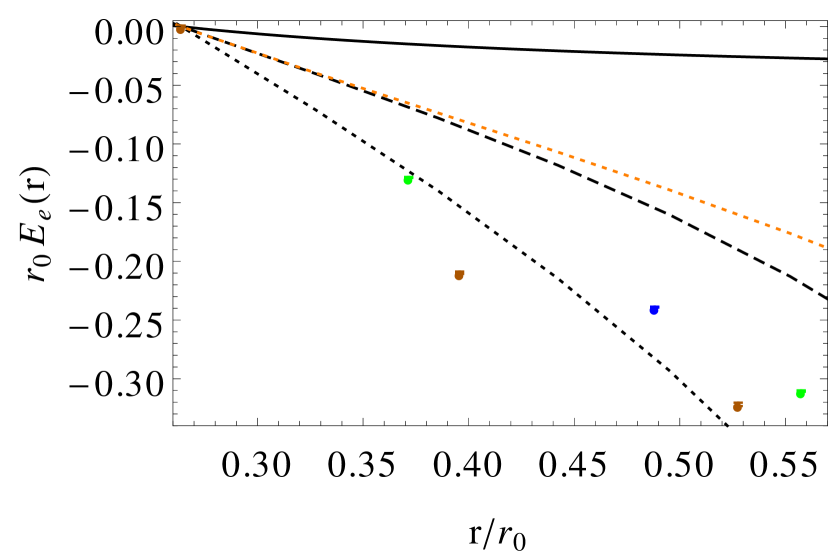
Figure 9: Comparison to the lattice data for $E_{e}$. The solid black line corresponds to the NLO result at fixed scale $\nu=2/0.263821r_{0}^{-1}$. The dashed black line corresponds to the NLO result setting $\nu=1/r$. The dotted lines correspond to the LL (orange) and NLL (black) results setting $\nu_{us}=C_{A}\alpha(\nu)/r$ and $\nu=1/r$.

The situation for $E_{e}$ is similar. Setting $\nu$ constant the agreement is bad, as can be seen in Figure 9. If we set $\nu=1/r$ the agreement is much better (optimal for $x\approx 0.83$). One can also find good agreement if we resum the ultrasoft logs for reasonable values of $x$ and $x_{us}$. Again, the uncertainties due to scale variations in the $r$ range where lattice data is available are sizable and prevent a more quantitative analysis.

Overall, we find that for all studied observables our predictions can be made compatible with the available lattice data. With this statement we mean that for (more or less) reasonable values of the factorization scale we can get reasonable agreement with the lattice data, and/or that the expected size of higher order corrections is large enough to accommodate the difference to the lattice data. We cannot make quantitative statements though. Whereas adjusting the factorization scale or incorporating the resummation of logarithms can improve the agreement with the lattice data in some cases, we do not observe a general pattern for all potentials. Estimates of higher order effects from scale variations produce large effects, related to the fact that we have evaluated our predictions at quite low scales (large distances). Also, as already mentioned, the lattice data is rather scarce. Still, we find it quite remarkable that the asymptotic behavior (the sign of the slope) predicted by the ultrasoft logarithms $\propto\ln(C_{A}\alpha)$ in $E_{d}$ and $E_{e}$ complies with the lattice data.

4.2 Long distances

It is also interesting to consider the long-distance behavior of the quasi-static energies. Their behavior cannot be predicted by QCD using analytic tools. Still, it can be simulated by computations in the discretized version of QCD, i.e. on the lattice. One can then compare these numerical results with model predictions. Here we focus on the effective string theory predictions for the $1/m$ and the SI momentum-dependent quasi-static energies obtained in Ref. PerezNadal:2008vm . For the SI momentum-dependent quasi-static energies, they are actually equivalent to the predictions obtained first with the minimal area law Barchielli:1986zs . The latter however misses the $1/m$ potential. The string model gives the following results at leading order in the $1/(r\Lambda_{\rm QCD})$ expansion:

$$E^{(1,0)} =\frac{\sigma}{2\pi}\ln(\sigma r^{2})+\mu_{1},$$ (83)

$$E_{b}(r) =E_{e}(r)=-\frac{r\sigma}{9},$$ (84)

$$E_{c}(r) =E_{d}(r)=-\frac{r\sigma}{6}.$$ (85)

These expressions only depend on the string tension $\sigma$. The string tension can be obtained from fits to the static potential at long distances. The number we use is taken from Necco:2001xg and reads: $\sigma=1.3882r_{0}^{2}$. Therefore, the above expressions are in fact predictions. On the lattice side, to obtain absolute normalizations is problematic. Hence, just like at short distances we compare energy differences. We choose to normalize our prediction to the longest distance (rightmost) lattice point available, where the above models are expected to work best. The comparison with the lattice is shown in Figures 10, 11 and 12. There is qualitative agreement between the lattice and the effective string theory predictions. On the other hand it is evident that the agreement is far from perfect and the slopes demand for corrections to the leading string behavior. Such corrections can in principle be computed in the same way as for the static potential, where they give rise to the Lüscher term Luscher:1980fr . It would be interesting to see if the analogous computations for the quasi-static energies (in case they happen to be free of new constants) improve the agreement with the lattice data.

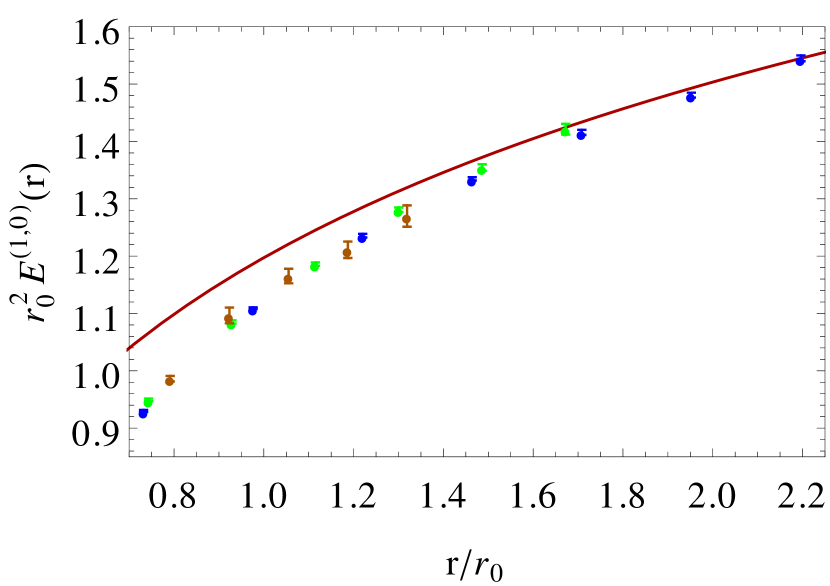
Figure 10: Comparison of the lattice data with the predictions from effective string theory at long distances for $E_{1}^{(1,0)}$.

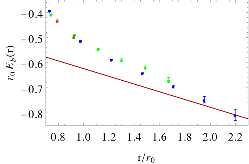
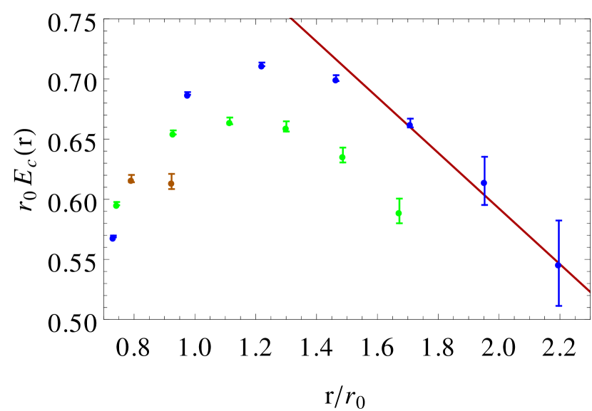
Figure 11: Comparison of the lattice data with the predictions from effective string theory at long distances for $E_{b}$ and $E_{c}$.

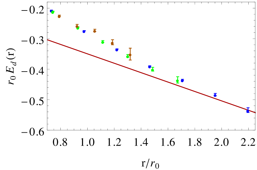
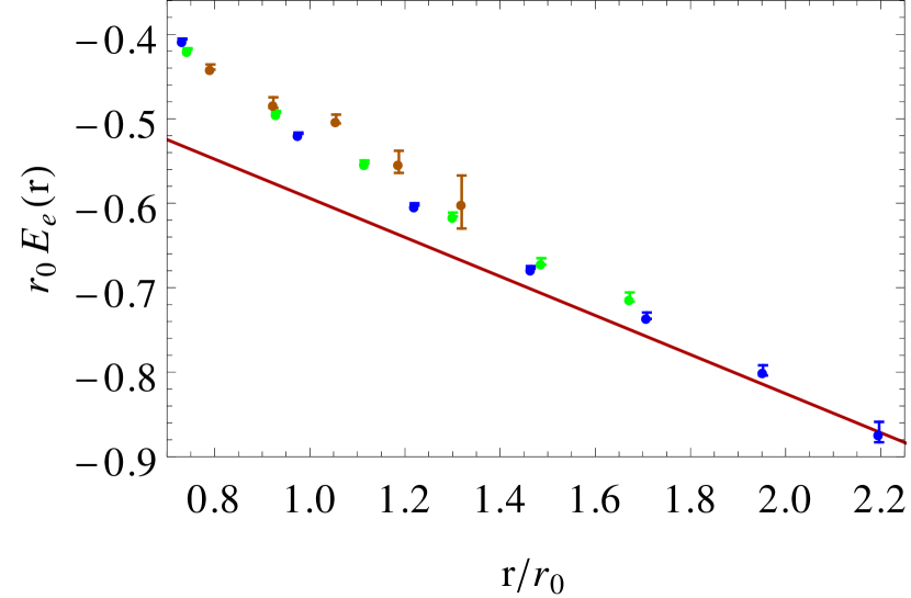
Figure 12: Comparison of the lattice data with the predictions from effective string theory at long distances for $E_{d}$ and $E_{e}$.

5 Conclusions

In this paper we have determined the short-distance behavior of the nonperturbative generalizations of the $1/m$ potential and of the $1/m^{2}$ SI momentum-dependent heavy quarkonium potentials, in terms of Wilson loops (as defined in Section 2.1), with ${\mathcal{O}}(\alpha^{3})$ and ${\mathcal{O}}(\alpha^{2})$ accuracy, respectively. We refer to these objects as quasi-static energies. Our results can be found in Eqs. (38)-(2.1). For our (NLO) computation it is crucial that the quasi-static energies start to be sensitive to the ultrasoft scale $\sim C_{A}\alpha/r$. Therefore, their calculation requires a resummation of an infinite number of potential interactions to account for the ultrasoft effects.

We have computed these ultrasoft contributions to the quasi-static energies in a diagrammatic approach. This included Feynman graphs with one ultrasoft and up to three potential loops. We expect that a proper EFT setup will significantly simplify such computations. At the same time this would allow for a systematic RG analysis beyond LL precision. With our method we were able perform the correct LL resummation of ultrasoft logarithms, but can only provide an educated guess for the NLL results.

Our results should reproduce the short-distance limit of lattice simulations of the same quasi-static energies. Some of these were evaluated long ago in Ref. Bali:1997am , and more recently in Refs. Koma:2006si ; Koma:2007jq ; Koma:2009ws . We have performed a preliminary comparison with the lattice data Koma:2006si ; Koma:2007jq ; Koma:2009ws at short distances in Section 4.1. As there is not enough lattice data at short distances, we were unable to perform a quantitative analysis. We had to compare at rather low scales. This causes large uncertainties from scale variations. Within these uncertainties we can find qualitative agreement with the data. It is quite remarkable that the sign of the slopes obtained by the lattice simulations agrees with the asymptotic behavior predicted by our weak coupling analysis. Whereas for three of the considered quasi-static energies, the behavior is dominated by the soft LO contribution, for two of them the sign of the slope is dictated by the ultrasoft contribution. This makes them particularly interesting. Those quasi-static energies vanish at ${\mathcal{O}}(\alpha)$, but are non-zero at ${\mathcal{O}}(\alpha^{2})$. Earlier lattice simulations predicted an approximately zero slope for them in the short distance limit. The most recent simulations show a non-zero behavior consistent with our results, albeit within large uncertainties.

We also compare the lattice data with the expectations from effective string models at long distances. We find qualitative agreement, but there is obvious room for improvement. In the long term one could try to study (qualitatively) how the short and long distance predictions (for a specific model) combine.

Acknowledgments
We thank Yoshiaki and Miho Koma for providing us with the lattice data of Refs. Koma:2007jq ; Koma:2009ws . A.P. thanks Gunnar S. Bali for discussions. M.S. is supported by GFK and by the PRISMA cluster of excellence at JGU Mainz. This work was supported in part by the Spanish grants FPA2014-55613-P, FPA2013-43425-P and SEV-2012-0234, and the Catalan grant SGR2014-1450.

Appendix A Results for the ultrasoft diagrams

For each diagram $X$ in Figure 1 (and equivalently in Figure 2) we have computed the object ${\cal W}_{n}^{X,ij}$ according to Eq. (28), in both Coulomb and Feynman gauge. The bare results in Feynman gauge (FG) read:

$${\cal W}_{n,\rm FG}^{1a,ij} =(-i)^{n+1}\frac{C_{F}}{2}\,g^{2}\delta^{ij}\Delta V^{D-n-1}(D-1)\pi^{-D/2}$$

$$\times\Gamma\left(\frac{D}{2}\right)\Gamma(1-D+n)\,,$$ (86)

$${\cal W}_{n,\rm FG}^{1b,ij} =-(-i)^{n+1}\frac{C_{F}}{2}\,g^{2}\delta^{ij}\Delta V^{D-n-1}\pi^{-D/2}$$

$$\times\Gamma\left(\frac{D}{2}\right)\Gamma(1-D+n)\,,$$ (87)

$${\cal W}_{n,\rm FG}^{2a,ij} =(-i)^{n+1}C_{A}C_{F}\,g^{4}\Big{(}(D-3){\hat{\bf r}}^{i}{\hat{\bf r}}^{j}-\delta^{ij}\Big{)}r^{3-D}$$

$$\times\Delta V^{D-n-2}(D-2)2^{-D}\pi^{1-D}\Gamma(D-3)\Gamma(2-D+n)\,,$$ (88)

$${\cal W}_{n,\rm FG}^{2b,ij} =(-i)^{n+1}C_{A}C_{F}\,g^{4}\delta^{ij}r^{3-D}\Delta V^{D-n-2}(D-2)$$

$$\times 2^{-D}\pi^{1-D}\Gamma(D-3)\Gamma(2-D+n)\,,$$ (89)

$${\cal W}_{n,\rm FG}^{2c,ij} =-(-i)^{n+1}C_{A}C_{F}\,g^{4}{\hat{\bf r}}^{i}{\hat{\bf r}}^{j}r^{3-D}\Delta V^{D-n-2}$$

$$\times\frac{2^{-D}\pi^{1-D}}{n+1}\Gamma(D-1)\Gamma(2-D+n)\,,$$ (90)

$${\cal W}_{n,\rm FG}^{3a,ij} =-(-i)^{n+1}C_{A}^{2}C_{F}\,g^{6}\Big{(}(D-5)(D-3){\hat{\bf r}}^{i}{\hat{\bf r}}^{j}+\delta^{ij}\Big{)}$$

$$\times r^{6-2D}\Delta V^{D-n-3}4^{-D}\pi^{1-\frac{3D}{2}}\sin\left(\frac{\pi D}{2}\right)$$

$$\times\Gamma\left(2-\frac{D}{2}\right)\Gamma^{2}(D-3)\Gamma(3-D+n)\,,$$ (91)

$${\cal W}_{n,\rm FG}^{3b,ij} =-(-i)^{n+1}C_{A}^{2}C_{F}\,g^{6}\delta^{ij}r^{6-2D}\Delta V^{D-n-3}4^{-D}\pi^{1-\frac{3D}{2}}$$

$$\times\sin\left(\frac{\pi D}{2}\right)\Gamma\left(2-\frac{D}{2}\right)\Gamma^{2}(D-3)\Gamma(3-D+n)\,,$$ (92)

$${\cal W}_{n,\rm FG}^{3c,ij} =-(-i)^{n+1}C_{A}^{2}C_{F}\,g^{6}\Big{(}(D-3){\hat{\bf r}}^{i}{\hat{\bf r}}^{j}-\delta^{ij}\Big{)}r^{6-2D}$$

$$\times\Delta V^{D-n-3}2^{1-2D}\pi^{1-\frac{3D}{2}}$$

$$\times\sin\left(\frac{\pi D}{2}\right)\Gamma\left(2-\frac{D}{2}\right)\Gamma^{2}(D-3)\Gamma(3-D+n)\,,$$ (93)

$${\cal W}_{n,\rm FG}^{3d,ij} =-(-i)^{n+1}C_{A}^{2}C_{F}\,g^{6}{\hat{\bf r}}^{i}{\hat{\bf r}}^{j}r^{6-2D}\Delta V^{D-n-3}$$

$$\times\frac{4^{1-D}\pi^{1-\frac{3D}{2}}}{n+1}\sin\left(\frac{\pi D}{2}\right)\Gamma\left(3-\frac{D}{2}\right)$$

$$\times\Gamma(D-4)\Gamma(D-1)\Gamma(3-D+n)\,,$$ (94)

$${\cal W}_{n,\rm FG}^{3e,ij} =(-i)^{n+1}C_{A}^{2}C_{F}\,g^{6}{\hat{\bf r}}^{i}{\hat{\bf r}}^{j}r^{4-2D}\Delta V^{D-n-5}$$

$$\times\frac{4^{-D}\pi^{1-\frac{3D}{2}}}{(n+1)(n+2)}\sin\left(\frac{\pi D}{2}\right)\Gamma\left(2-\frac{D}{2}\right)$$

$$\times\Gamma^{2}(D-2)\Gamma(3-D+n)$$

$$\times\big{[}(D-2)\Delta V^{2}r^{2}-2(D-n-4)(D-n-3)\big{]}\,,$$ (95)

$${\cal W}_{n,\rm FG}^{3f,ij} =(-i)^{n+1}C_{A}^{2}C_{F}\,g^{6}{\hat{\bf r}}^{i}{\hat{\bf r}}^{j}r^{4-2D}\Delta V^{D-n-5}\frac{4^{-D}\pi^{1-\frac{3D}{2}}}{\Gamma(n+3)}$$

$$\times\sin\left(\frac{\pi D}{2}\right)\Gamma\left(2-\frac{D}{2}\right)\Gamma^{2}(D-2)$$

$$\times\Gamma(n+1)\Gamma(5-D+n)\,,$$ (96)

$${\cal W}_{n,\rm FG}^{3g,ij} ={\cal W}_{n,\rm FG}^{3f,ij}\,,$$ (97)

$${\cal W}_{n,\rm FG}^{4a,ij} =-(-i)^{n+1}C_{A}^{3}C_{F}\,g^{8}{\hat{\bf r}}^{i}{\hat{\bf r}}^{j}r^{9-3D}\Delta V^{D-n-4}$$

$$\times\frac{2^{2-3D}\pi^{1-2D}}{n+1}\sin^{2}\left(\frac{\pi D}{2}\right)$$

$$\times\Gamma^{2}\left(2-\frac{D}{2}\right)\Gamma^{2}(D-3)\Gamma(D-2)\Gamma(4-D+n)\,,$$ (98)

$${\cal W}_{n,\rm FG}^{4b,ij} =-(-i)^{n+1}C_{A}^{3}C_{F}\,g^{8}{\hat{\bf r}}^{i}{\hat{\bf r}}^{j}r^{9-3D}\Delta V^{D-n-4}$$

$$\times\frac{2^{4-3D}\pi^{1-2D}}{n+1}\sin^{2}\left(\frac{\pi D}{2}\right)\Gamma^{2}\left(3-\frac{D}{2}\right)$$

$$\times\Gamma(D-4)\Gamma(D-3)\Gamma(D-2)\Gamma(4-D+n)\,,$$ (99)

$${\cal W}_{n,\rm FG}^{5a,ij} =-(-i)^{n+1}C_{A}^{4}C_{F}\,g^{10}{\hat{\bf r}}^{i}{\hat{\bf r}}^{j}r^{12-4D}\Delta V^{D-n-5}$$

$$\times\frac{2^{4-4D}\pi^{1-\frac{5D}{2}}\Gamma(n+1)}{\Gamma(n+3)}\sin^{3}\left(\frac{\pi D}{2}\right)\Gamma\left(2-\frac{D}{2}\right)$$

$$\times\Gamma^{2}\left(3-\frac{D}{2}\right)\Gamma^{2}(D-4)\Gamma^{2}(D-2)\Gamma(5-D+n)\,,$$ (100)

where $D=d+1=4+2\epsilon$ and ${\hat{\bf r}}={\bf r}/r$. Using Eq. (27) the sum of the ${\cal W}_{n,\rm FG}^{X,ij}$ gives the gauge invariant result in Eq. (36).

In Coulomb gauge (CG) we obtain:

$${\cal W}_{n,\rm CG}^{X,ij} =\frac{D-2}{D-1}\;{\cal W}_{n,\rm FG}^{X,ij}$$

$$\text{for}\quad X=\{1a,2a,2b,3a,3b,3c,3d,4a,4b,5a\}\,,$$ (101)

$${\cal W}_{n,\rm CG}^{Y,ij} =0$$

$$\text{for}\quad Y=\{1b,2c,3e,3f,3g\}\,.$$ (102)

The fact that the sum of the ${\cal W}_{n,\rm CG}^{X,ij}$ gives again the gauge invariant result in Eq. (36) is a strong cross check of our computation.

References

- (1) A. Pineda and J. Soto, Nucl. Phys. Proc. Suppl. 64, 428 (1998) [hep-ph/9707481].
- (2) N. Brambilla, A. Pineda, J. Soto and A. Vairo, Nucl. Phys. B 566, 275 (2000) [hep-ph/9907240].
- (3) N. Brambilla, A. Pineda, J. Soto and A. Vairo, Rev. Mod. Phys. 77, 1423 (2005) [hep-ph/0410047].
- (4) A. Pineda, Prog. Part. Nucl. Phys. 67 (2012) 735 [arXiv:1111.0165 [hep-ph]].
- (5) W. E. Caswell and G. P. Lepage, Phys. Lett. B 167, 437 (1986).
- (6) G. T. Bodwin, E. Braaten and G. P. Lepage, Phys. Rev. D 51, 1125 (1995) [Phys. Rev. D 55, 5853 (1997)] [hep-ph/9407339].
- (7) C. Peset, A. Pineda and M. Stahlhofen, JHEP 1605 (2016) 017 [arXiv:1511.08210 [hep-ph]].
- (8) B. A. Kniehl, A. A. Penin, V. A. Smirnov and M. Steinhauser, Nucl. Phys. B 635, 357 (2002) [hep-ph/0203166].
- (9) C. Anzai, Y. Kiyo and Y. Sumino, Phys. Rev. Lett. 104, 112003 (2010) [arXiv:0911.4335 [hep-ph]].
- (10) A. V. Smirnov, V. A. Smirnov and M. Steinhauser, Phys. Rev. Lett. 104, 112002 (2010) [arXiv:0911.4742 [hep-ph]].
- (11) S. N. Gupta and S. F. Radford, Phys. Rev. D 25, 3430 (1982).
- (12) B. A. Kniehl, A. A. Penin, M. Steinhauser and V. A. Smirnov, Phys. Rev. D 65, 091503 (2002) [hep-ph/0106135].
- (13) N. Brambilla, A. Pineda, J. Soto and A. Vairo, Phys. Rev. D 63 (2001) 014023 [hep-ph/0002250].
- (14) A. Pineda and A. Vairo, Phys. Rev. D 63 (2001) 054007 [Phys. Rev. D 64 (2001) 039902] [hep-ph/0009145].
- (15) K. G. Wilson, Phys. Rev. D 10, 2445 (1974).
- (16) A. Barchielli, E. Montaldi and G. M. Prosperi, Nucl. Phys. B 296, 625 (1988) Erratum: [Nucl. Phys. B 303, 752 (1988)].
- (17) N. Brambilla, M. Groher, H. E. Martinez and A. Vairo, Phys. Rev. D 90, no. 11, 114032 (2014) [arXiv:1407.7761 [hep-ph]].
- (18) Y. Koma, M. Koma and H. Wittig, Phys. Rev. Lett. 97, 122003 (2006) [hep-lat/0607009].
- (19) Y. Koma, M. Koma and H. Wittig, PoS LAT 2007, 111 (2007) [arXiv:0711.2322 [hep-lat]].
- (20) Y. Koma and M. Koma, PoS LAT 2009, 122 (2009) [arXiv:0911.3204 [hep-lat]].
- (21) G. S. Bali, K. Schilling and A. Wachter, Phys. Rev. D 56, 2566 (1997) [hep-lat/9703019].
- (22) T. Appelquist, M. Dine and I. J. Muzinich, Phys. Rev. D 17, 2074 (1978).
- (23) N. Brambilla, A. Pineda, J. Soto and A. Vairo, Phys. Rev. D 60, 091502 (1999) [hep-ph/9903355].
- (24) A. Pineda and M. Stahlhofen, Phys. Rev. D 81, 074026 (2010) [arXiv:1002.1965 [hep-th]].
- (25) A. A. Penin and M. Steinhauser, Phys. Lett. B 538, 335 (2002) [hep-ph/0204290].
- (26) C. Ayala, G. Cvetic and A. Pineda, JHEP 1409, 045 (2014) [arXiv:1407.2128 [hep-ph]].
- (27) Y. Kiyo, G. Mishima and Y. Sumino, Phys. Lett. B 752, 122 (2016) [arXiv:1510.07072 [hep-ph]].
- (28) A. Bazavov, N. Brambilla, X. Garcia i Tormo, P. Petreczky, J. Soto and A. Vairo, Phys. Rev. D 86, 114031 (2012) [arXiv:1205.6155 [hep-ph]].
- (29) J. K. Erickson, G. W. Semenoff, R. J. Szabo and K. Zarembo, Phys. Rev. D 61, 105006 (2000) [hep-th/9911088].
- (30) A. Pineda, Phys. Rev. D 77, 021701 (2008) [arXiv:0709.2876 [hep-th]].
- (31) M. Stahlhofen, JHEP 1211, 155 (2012) [arXiv:1209.2122 [hep-th]].
- (32) M. Prausa and M. Steinhauser, Phys. Rev. D 88, no. 2, 025029 (2013) [arXiv:1306.5566 [hep-th]].
- (33) D. Schaich, S. Catterall, P. H. Damgaard and J. Giedt, PoS LATTICE 2016, 221 (2016) [arXiv:1611.06561 [hep-lat]].
- (34) M. Beneke and V. A. Smirnov, Nucl. Phys. B 522, 321 (1998) [hep-ph/9711391].
- (35) A. Barchielli, N. Brambilla and G. M. Prosperi, Nuovo Cim. A 103, 59 (1990).
- (36) J. G. M. Gatheral, Phys. Lett. 133B, 90 (1983).
- (37) J. Frenkel and J. C. Taylor, Nucl. Phys. B 246, 231 (1984).
- (38) Y. Schroder, DESY-THESIS-1999-021.
- (39) A. Pineda, Phys. Rev. D 84, 014012 (2011) [arXiv:1101.3269 [hep-ph]].
- (40) M. E. Luke, A. V. Manohar and I. Z. Rothstein, Phys. Rev. D 61, 074025 (2000) [hep-ph/9910209].
- (41) A. H. Hoang and M. Stahlhofen, Phys. Rev. D 75 (2007) 054025 [hep-ph/0611292].
- (42) A. H. Hoang and M. Stahlhofen, JHEP 1106, 088 (2011) [arXiv:1102.0269 [hep-ph]].
- (43) A. Pineda and J. Soto, Phys. Lett. B 495, 323 (2000) [hep-ph/0007197].
- (44) N. Brambilla, A. Vairo, X. Garcia i Tormo and J. Soto, Phys. Rev. D 80, 034016 (2009) [arXiv:0906.1390 [hep-ph]].
- (45) A. Pineda and M. Stahlhofen, Phys. Rev. D 84, 034016 (2011) [arXiv:1105.4356 [hep-ph]].
- (46) A. Pineda, Phys. Rev. D 65, 074007 (2002) [hep-ph/0109117].
- (47) A. Pineda, J. Phys. G 29, 371 (2003) [hep-ph/0208031].
- (48) G. Perez-Nadal and J. Soto, Phys. Rev. D 79, 114002 (2009) [arXiv:0811.2762 [hep-ph]].
- (49) N. Brambilla and A. Vairo, Phys. Rev. D 55, 3974 (1997) [hep-ph/9606344].
- (50) S. Necco and R. Sommer, Nucl. Phys. B 622, 328 (2002) [hep-lat/0108008].
- (51) M. Luscher, K. Symanzik and P. Weisz, Nucl. Phys. B 173, 365 (1980).