Fiducial on a string
Revisiting Fisher’s fiducial inference
Abstract
The fiducial argument of Fisher (1973) has been described as his biggest blunder, but the recent review of Hannig et al. (2016) demonstrates the current and increasing interest in this brilliant idea. This short note analyses an example introduced by Seidenfeld (1992) where the fiducial distribution is restricted to a string.
keywords:
and
1 The problem
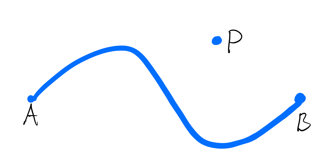
Assume that a fiducial distribution located at has been derived, but that it is known that the parameter lies on a string connecting points and as illustrated in Figure 1.
Fisher (1973, p.138-142) considers this problem for the particular case where the initial fiducial is bivariate normal with mean . For the case of a straight line and a circle he derives a fiducial from sufficiency and ancilarity respectively. For the general case Fisher (1973, p.142) indicates that the fiducial can be calculated from the likelihood for each point on the curve.
Seidenfeld (1992, Example 5.1) considers the case where the observations are given by
| (1) |
where , , and is drawn from . Using Bayes’ theorem argumentation he arrives at two contradicting fiducial distributions. The first corresponds to the Bayes posterior from a uniform prior law for , and the other corresponds to a uniform prior law for . Seidenfeld (1992, p.367) notes that this example is challenging for a wide variety of what Savage called “necessitarian” theories: Theories that try to find privileged distributions to represent “ignorance”.
2 Conditional fiducial inference
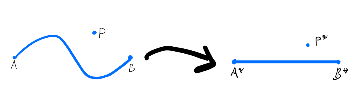
The problem for the line segment can be solved by introducing coordinates such that the line segment is given by and . A fiducial on a string is then determined by the conditional law
| (2) |
If has a derivative and the initial fiducial is given by a probability density , then the conditional law will have a density proportional to where
| (3) |
The initial fiducial from equation (1) is given by where is sampled from the bivariate normal density . The initial density of is then . A particularly simple transformation is given on the form with , , and . The resulting density for is then proportional to
| (4) |
The last factor is the component of orthogonal to . It is proportional to evaluated at . The two alternative fiducial distributions obtained by Seidenfeld (1992) are given by corresponding to shifts in the two coordinate directions. Generally, restricted to the simple transformation form, the last factor is proportional to any non-zero linear combination of the coordinates of . A more general solution is given by equation (3).
3 A fiducial argument
Assume that an initial fiducial model is given by a quasi-group multiplication (Taraldsen and Lindqvist, 2013)
| (5) |
In this case, the fiducial distribution of is obtained by making the judgment that it equals its original sampling distribution. The initial fiducial distribution of is then uniquely determined by equation (5) when is the fixed observed value and is from its original sampling distribution.
Consider now as previously that is restricted to values with for an underlying parameter . This gives, for a fixed observed , a corresponding parameterization of possible values of determined by equation (5). Introduce now a transformation so that the restriction on corresponds to and . The resulting fiducial distribution for after observing is then the conditional distribution
| (6) |
If has a derivative and the initial fiducial is given by a probability density , then the conditional law will have a density proportional to , where
| (7) |
This is in complete analogy with equation (3), and leads in particular to the two fiducial distributions of Seidenfeld (1992) as before by consideration of a transformation on the form for this additive group case. The transformation depends in this case explicitly on .
The results so far correspond to and a formal Bayes prior density for on the form
| (8) |
Equation (4) corresponds to a case where does not depend on , but equation (3) corresponds to a case with dependence of . Equation (7) can lead to cases where the weight also depends on : A data dependent prior. This is as described more generally by Hannig et al. (2016) using a different, but related approach.
The Jeffreys prior is on the form
| (9) |
The fiducial resulting from the arguments leading to equation (8) will always lead to a proper posterior as dictated by equations (5-6). If equation (5) corresponds to a locally compact group, then the initial fiducial is a Bayes posterior and the final fiducial resulting from equation (8) is then also a Bayes posterior.
4 Discussion and conclusion
This note was initiated due to comments from Teddy Seidenfeld during the 4th Bayesian, Fiducial and Frequentist (BFF4) workshop at Harvard University in May 2017. We gave an invited talk where the concept of a conditional fiducial model was presented: A fiducial model together with a condition (Taraldsen and Lindqvist, 2017). The fiducial is not uniquely given by the additional demand that the parameter is restricted to be on a given curve. It is, however, uniquely given if this is reformulated by a condition . In the setting given by this note, it follows that it corresponds to a formal prior on the form
| (10) |
Note that is a normal vector to the curve tangent vector , and that it is possible to choose a path-length parameterisation so that . A condition with constant on the curve gives the Jeffreys prior in equation (9), and other choices give the general result corresponding to equation (3).
We hereby acknowledge most fruitful discussions with Teddy Seidenfeld, Jan Hannig, and the other participants at the Harvard BFF4 workshop.
References
- Fisher (1973) {bbook}[author] \bauthor\bsnmFisher, \bfnmR. A.\binitsR. A. (\byear1973). \btitleStatistical methods and scientific inference. \bpublisherHafner press. \endbibitem
- Hannig et al. (2016) {barticle}[author] \bauthor\bsnmHannig, \bfnmJ.\binitsJ., \bauthor\bsnmIyer, \bfnmH.\binitsH., \bauthor\bsnmLai, \bfnmR. C. S.\binitsR. C. S. and \bauthor\bsnmLee, \bfnmT. C. M.\binitsT. C. M. (\byear2016). \btitleGeneralized Fiducial Inference: A Review and New Results. \bjournalJournal of the American Statistical Association \bvolume111 \bpages1346-1361. \endbibitem
- Seidenfeld (1992) {barticle}[author] \bauthor\bsnmSeidenfeld, \bfnmTeddy\binitsT. (\byear1992). \btitleR. A. Fisher’s Fiducial Argument and Bayes’ Theorem. \bjournalStatistical Science \bvolume7. \bdoi10.2307/2246072 \endbibitem
- Taraldsen and Lindqvist (2013) {barticle}[author] \bauthor\bsnmTaraldsen, \bfnmG.\binitsG. and \bauthor\bsnmLindqvist, \bfnmB. H.\binitsB. H. (\byear2013). \btitleFiducial theory and optimal inference. \bjournalAnnals of Statistics \bvolume41 \bpages323–341. \endbibitem
- Taraldsen and Lindqvist (2017) {barticle}[author] \bauthor\bsnmTaraldsen, \bfnmG.\binitsG. and \bauthor\bsnmLindqvist, \bfnmB. H.\binitsB. H. (\byear2017). \btitleConditional fiducial models. \bjournalJournal of Statistical Planning and Inference \bvolume(accepted). \endbibitem