A continuous-variable approach to the spectral properties and quantum states
of the two-component Bose-Hubbard dimer

Abstract

A bosonic gas formed by two interacting species trapped in a double-well potential features macroscopic localization effects when the interspecies interaction becomes sufficiently strong. A repulsive interaction spatially separates the species into different wells while an attractive interaction confines both species in the same well. We perform a fully-analytic study of the transitions from the weak- to the strong-interaction regime by exploiting the semiclassical method in which boson populations are represented in terms of continuous variables. We find an explict description of low-energy eigenstates and spectrum in terms of the model parameters which includes the neighborhood of the transition point. To test the effectiveness of the continuous-variable method we compare its predictions with the exact results found numerically. Numerical calculations confirm the spectral collapse evidenced by this method when the space localization takes place.

I Introduction

Many-boson systems described in the Bose-Hubbard picture are characterized by density-density interactions whose nonlinear character determines an extraordinarily rich scenario of dynamical behaviors and properties. In this framework and among many interesting aspects, a large attention has been focused on small-size bosonic lattices since they provide a fertile ground to investigate the quantum-classical correspondence and the role of nonlinear interactions rev1 -rev12 . While the semiclassical approaches sc1 -sc3 to this class of systems are generally not problematic, their study at the purely-quantum level remains a considerably hard task and the diagonalization of quantum Hamiltonians mainly relies on the use of numerical techniques.

An effective analytical method which has allowed, in many situations, to circumvent this difficulty consists in reformulating the dynamics of low-energy bosonic states in terms of continuous variables (CV) which represent the quantum numbers of boson populations. Fock states are thus transformed in wave functions depending on the CV while the energy-eigenvalue equation can be reduced, in the low-energy regime, to the problem of a multidimensional harmonic oscillator.

This scheme has found large application in the last two decades for studying the spatial fragmentation cvp1 and the spectral properties cvp3 of condensates trapped in a double-well potential, the critical behavior cvp4 and the dynamical phase transition cvp5 , cvp6 leading to the emergence of localized ground states in attractive condensates, and the collapse and revival cvp7 of nonlinear tunneling in Bose-Hubbard (BH) chains.

While the CV approximation can be directly carried out on the energy-state eigenvalue problem to reduce it to a solvable differential equation as in papers cvp1 -cvp7 , a simple but useful generalization of this method consists in the derivation of an effective Hamiltonian associated with the original model. This has been used to reduce the BH chain to a solvable phonon-like quadratic Hamiltonian cvp8 , and to show how the potential provided by the effective Hamiltonian completely determines the ground-state properties of the attractive BH trimer cvp9 and of a gas of dipolar bosons in a four-well ring cvp10 .

In this paper we apply the CV method to reproduce the mechanism governing the spectral collapse of energy levels, a phenomenon which often marks critical phenomena involving the transition to new dynamical regimes. This is the case for nonlinear BH-like models but also for models describing matter-photon interactions whose nonlinearity is inherent in the spinor form of their Schrödinger problem. Several examples are known such as the transition to the super-radiant phase in the Dicke model, exhibiting the emergence of a quasicontinuous spectrum Em , and the interaction-induced spectral collapse characterizing the two-photon quantum Rabi model Fe in which the Hamiltonian becomes unitarily equivalent to a noncompact generator of su(1,1) PeRa .

The same effect distinguishes as well the transition of single-depleted-well states from stable to unstable regimes in the BH trimer rev10 , VP , and the emergence from the delocalization regime of a fully-localized ground state in a double-well system (dimer) with two bosonic components LMP . The dimer system involving binary mixtures has recently raised a considerable interest, and its dynamical stability xu , different types of self-trapping solutions satjia , the Rabi-Josephson dynamics mazz2011 , the low-energy quantum states citro , and the interspecies entanglement properties mujal have been investigated. A more extensive discussion on the nonlinear dynamics of multicomponent systems described in terms of discrete nonlinear Schrödinger equations and of their modulational instability can be found in baizakov -kevre .

In reference LMP , the two-component BH dimer has been investigated and its exact spectrum has been compared with the spectrum derived through a Bogoliubov-like scheme. The derivation of the latter, however, revealed how the implementation of this semiclassical approximation strongly depends on the dynamical regime in which is performed. More specifically, different dynamical regimes involve totally different sets of microscopic bosonic modes enabling the diagonalization process. In addition, the complex structure of the energy eigenstates resulting from this process is such that extracting the significant physical information often is a non trivial task.

In this paper, the CV method is shown to offer a unified effective scheme able to determine the spectrum for any choice of the model parameters, and to supply a complete description of the spectral collapse emerging in the transition from the weak to strong-interaction regime. The study of a model including the occurrence of a known critical phenomenon allows us to better test the effectiveness of this method, a central aspect of this work.

After deriving the effective Hamiltonian for the two-component dimer in terms of continuous variables and the relevant minimum-energy configurations, we apply the CV method to reconstruct the energy levels of the systems and the explicit expression of the corresponding eigenstates. We demonstrate as well how this methodology effectively describes, in a fully analytic way, the mechanism of the transition (heralded by the spectral collapse) from a ground state with delocalized boson populations to a ground state where boson populations become strongly localized.

In Section II we review the CV method and derive the model Hamiltonian for the two-component dimer Hamiltonian within this scheme. Section III is devoted to solve the boson-population equations incorporating the information about the minimum-energy configurations. In Section IV, we reconstruct the spectrum and the eigenstates. Finally, Section V is devoted to compare exact results, found numerically, with the spectrum and the eigenstates derived through the CV method.

I.1 The 2-component dimer model

Ultracold bosons trapped in two potential wells are well described by the two-mode BH Hamiltonian

$$H_{a}=\frac{U_{a}}{2}\Bigl{[}a_{L}^{\dagger}a_{L}^{\dagger}a_{L}a_{L}+a_{R}^{+}a_{R}^{+}a_{R}a_{R}\Bigr{]}-J_{a}\big{(}a_{L}^{+}a_{R}+a_{R}^{+}a_{L}\big{)},$$

where $L$ ($R$) refers to the left (right) well, and the boson operators $a_{L}$, $a_{L}^{+}$, $a_{R}$, $a_{R}^{+}$ satisfy the standard commutator $[a_{\sigma},a_{\sigma}^{+}]$ $=1$ with $\sigma=L,R$. Parameters $U_{a}$ and $J_{a}$ are the boson-boson interaction and the hopping amplitude, respectively. In the presence of two interacting atomic species, the spatial modes become four, $a_{L}$, $a_{R}$, and $b_{L}$, $b_{R}$, for the components $A$ and $B$, respectively. The microscopic dynamics of the system is described by the two-species dimer Hamiltonian (TDH) defined on a two-site lattice

$$\hat{H}={H}_{a}+{H}_{b}+W\big{(}a^{+}_{L}{a}_{L}b^{+}_{L}b_{L}+a^{+}_{R}{a}_{R}b^{+}_{R}{b}_{R}\big{)}$$ (1)

where ${H}_{a}$ and ${H}_{b}$ are the single-species Hamiltonians and the interspecies interaction $W$ describes the coupling of the two components. The further hopping parameter $J_{b}$ and intraspecies interaction $U_{b}$ occur in $H_{b}$ describing the second component. Since the total boson numbers

$$N_{a}=N_{aL}+N_{aR},\quad N_{b}=N_{bL}+N_{bR},$$

($N_{ar}=a^{+}_{r}{a}_{r}$, $N_{br}=b^{+}_{r}{b}_{r}$, $r=L,R$) of each bosonic component are conserved quantities being $[H,N_{a}]$ $=[H,N_{b}]$ $=0$, the eigenvalues of $N_{a}$ and $N_{b}$ represent two further significant parameters. We shall denote the boson numbers of the two species with the same symbols $N_{a}$ and $N_{b}$ of their number operators.

II The continuous-variable method

A useful description of the low-energy scenario of multimode bosonic models can be obtained by observing that physical quantities depending on the local populations $n_{i}$ (the eigenvalues of number operators $\hat{n}_{i}=\hat{c}^{\dagger}_{i}\hat{c}_{i}$) can be reformulated in terms of continuous variables $x_{i}=n_{i}/N$ representing local densities cvp1 -cvp4 . For boson number $N=\sum_{i}n_{i}$ large enough, Fock states $|{\vec{n}}\rangle=|n_{1},n_{2},...,n_{L}\rangle\equiv|x_{1},x_{2},...,x_{L}\rangle$, can be interpreted as functions of variables $x_{i}$ and creation/destruction processes $n_{i}\to n_{i}\pm 1$ correspond to small variations $|x_{1},...,x_{i}\pm\epsilon,...,x_{L}\rangle$ of state $|x_{1},...,x_{i},...,x_{L}\rangle$, where $\epsilon=1/N\ll 1$. Such an approach, in addition to simplify the energy-eigenvalue problem associated to a multimode Hamiltonian ${H}$, also leads to a new effective Hamiltonian written in terms of coordinates $x_{i}$ and of the corresponding generalized momenta cvp9 . A well-known example cvp10 is provided by the BH Hamiltonian defined on a one-dimensional lattice

$$\hat{H}=\frac{U}{2}{\sum}^{M}_{i=1}\hat{n}_{i}(\hat{n}_{i}-1)-J{\sum}_{rs}A_{rs}\hat{c}^{\dagger}_{r}\hat{c}_{s}\,,$$

where $M$ is the lattice-site number, $r,s\in[1,M]$ and the adjacency matrix $A_{rs}$ is equal to $1$ for $s=r\pm 1$ and zero in the other cases. By expanding up to the second order the quantity $\hat{H}|E\rangle$ in the corresponding eigenvalue problem $\hat{H}|E\rangle=E|E\rangle$, the latter takes the CVP form

$$(-D+V\,)\,\psi_{E}({\vec{x}})=\,{E}\,\psi_{E}({\vec{x}})\,,$$ (2)

including the generalized Laplacian

$$D=\,N^{2}U\tau\sum_{rs}\frac{\epsilon^{2}}{2}A_{rs}\,\Bigl{(}\partial_{r}-\partial_{s}\Bigr{)}\,{\sqrt{x_{r}\,x_{s}}}\Bigl{(}\partial_{r}-\partial_{s}\Bigr{)}\,,$$

with $\tau=J/(NU)$, and the effective potential

$$V=N^{2}U\sum^{M}_{r=1}\left(\frac{1}{2}x_{r}(x_{r}-\epsilon)-2\tau{\sqrt{x_{r}\,x_{r+1}}}\right)\,.$$

The solutions $\psi_{E}({\vec{x}})$ to problem (2) is easily found by considering the eigenvalues $E$ close to the extremal points (minima and maxima) of $V$ where the latter can be reduced to a quadratic form, namely, to a multidimensional harmonic oscillator. Once $\psi_{E}({\vec{x}})$ has been determined, the eigenstates of the original eigenvalue problem for $\hat{H}$ are found to be $|E\rangle=\sum_{\vec{x}}\psi_{E}({\vec{x}})|{\vec{x}}\rangle$. At the operational level, in addition to obtain an approximation of the energy spectrum which seems to be effective (this aspect has been explored in Ref. cvp9 for the attractive BH model), one can exploit potential $V$ to obtain significant information about the ground-state configurations and its characteristic regimes when the model parameters are varied. In the sequel, we focus our attention on $V$ and on the relevant extremal-point equations $\partial V/\partial{x_{i}}=0$ which allow to determine at each lattice site the boson populations characterizing the ground state.

II.1 The TDH in the continuous-variable picture

The application of the CV method to the TDH defined by (1) yields the new eigenvalue equation

$${\cal H}\,\psi_{E}({\vec{x}},{\vec{y}})=\,{E}\,\psi_{E}({\vec{x}},{\vec{y}})\;,$$ (3)

where ${\vec{x}}=(x_{R},x_{L})$ and ${\vec{y}}=(y_{R},y_{L})$ and $x_{k}=n_{k}/N_{a}$ and $y_{k}=m_{k}/N_{b}$ with $k=L,R$ describe the populations of species $a$ and $b$, respectively, Concerning $N_{a}$ and $N_{b}$ one should recall that the total boson number $N_{a}=n_{L}+n_{R}$ and $N_{b}=m_{L}+m_{R}$ of the two species are conserved quantities. $\cal H$ contains the generalized Laplacian $D=D_{x}+D_{y}$ in which, in addition to

$$D_{x}=\;N_{a}J_{a}\epsilon_{a}^{2}\Bigl{(}\partial_{x_{L}}-\partial_{x_{R}}\Bigr{)}\,{\sqrt{x_{L}\,x_{R}}}\Bigl{(}\partial_{x_{L}}-\partial_{x_{R}}\Bigr{)}\,,$$

one must include $D_{y}$, due to the second component. $D_{y}$ is found by replacing $N_{a}U_{a}\epsilon_{a}^{2}$ with $N_{b}J_{b}\epsilon_{b}^{2}$ and $x$ with $y$, where $\epsilon_{r}=1/N_{r}$ and $r=a,b$. Then ${\cal H}$ becomes

$${\cal H}=\tau_{a}\epsilon_{a}^{2}\Bigl{(}\partial_{x_{L}}-\partial_{x_{R}}\Bigr{)}\,{\sqrt{x_{L}\,x_{R}}}\Bigl{(}\partial_{x_{L}}-\partial_{x_{R}}\Bigr{)}$$

$$+\tau_{b}\epsilon_{b}^{2}\Bigl{(}\partial_{y_{L}}-\partial_{y_{R}}\Bigr{)}\,{\sqrt{y_{L}\,y_{R}}}\Bigl{(}\partial_{x_{L}}-\partial_{x_{R}}\Bigr{)}+\;V$$

whose potential $V$ has the form

$$V=-\gamma+\frac{u_{a}}{2}\Bigl{(}x^{2}_{L}+x^{2}_{R}\Bigr{)}+\frac{u_{b}}{2}\Bigl{(}y^{2}_{L}+y^{2}_{R}\Bigr{)}$$

$$+w(x_{L}y_{L}+x_{R}y_{R})-2\Bigl{(}\tau_{a}{\sqrt{x_{R}\,x_{L}}}+\tau_{b}{\sqrt{y_{R}\,y_{L}}}\Bigr{)}\;.$$

In $V$ the new parameters $\gamma=(U_{a}N_{a}+U_{b}N_{b})/2$ and

$$w=WN_{a}N_{b}\;,\quad\tau_{k}=J_{k}N_{k}\;,\quad u_{k}=N^{2}_{k}U_{k}\;,$$ (4)

with $k=a,b$, have been used. The conservation of boson populations $N_{a}$ and $N_{b}$, represented by equations $1=x_{R}+x_{L}$, and $1=y_{R}+y_{L}$ implies that two of the four coordinates $x_{i}$ and $y_{j}$ can be seen as dependent variables. By introducing the new population-imbalance variables $x=x_{L}-x_{R}$ and $y=y_{L}-y_{R}$ the bosonic populations are thus described by $x_{L}=(1+x)/2$, $x_{R}=(1-x)/2$, $y_{L}=(1+y)/2$, and $y_{R}=(1-y)/2$ while the effective Hamiltonian (EH) takes the form

$${\cal H}=-D-\gamma+\frac{u_{a}}{4}\Bigl{(}1+x^{2}\Bigr{)}+\frac{u_{b}}{4}\Bigl{(}1+y^{2}\Bigr{)}$$

$$+\frac{w}{2}(1+xy)-\Bigl{(}\tau_{a}{\sqrt{1-x^{2}}}+\tau_{b}{\sqrt{1-y^{2}}}\Bigr{)}\;.$$ (5)

with the Laplacian

$$D\simeq 2\tau_{a}\epsilon_{a}^{2}\sqrt{1-{\bar{x}}^{2}}\frac{\partial^{2}}{\partial x^{2}}+2\tau_{b}\epsilon_{b}^{2}\sqrt{1-{\bar{y}}^{2}}\frac{\partial^{2}}{\partial y^{2}}\;.$$

The operator $D$ has been approximated by introducing the quantities ${\bar{x}}$ and ${\bar{y}}$ representing the values of $x$ and $y$ for which $V$ reachs one of its extremal values and the EH essentially reduces to a model of coupled harmonic oscillators.

II.2 The semiclassical picture of TDH

It is interesting to highlight the link of TDH reduced to the form (5) with the semiclassical version of TDH which exhibits, as the most part of multimode boson models, a dynamics typically described by discrete nonlinear Schrödinger equations kevre . The semiclassical picture, in which boson operators $a_{r}$ and $b_{r}$ are replaced by local order parameters $\alpha_{r}$, and $\beta_{r}$ ($r=$ $L,R$), and the semiclassical Hamiltonian $H_{s}$ associated to (1) are discussed in Appendix A. $H_{s}$ takes the form (23)

$${H}_{s}=\frac{u_{a}}{4}\Bigl{(}1+x^{2}\Bigr{)}+\frac{u_{b}}{4}\Bigl{(}1+y^{2}\Bigr{)}+\frac{w}{2}(1+xy)$$

$$-\Bigl{(}\tau_{a}{\sqrt{1-x^{2}}}\cos(2\theta_{x})+\tau_{b}{\sqrt{1-y^{2}}}\cos(2\theta_{y})\Bigr{)}\;,$$

where $x=(|\alpha_{L}|^{2}-|\alpha_{R}|^{2})/N_{a}$, $y=(|\beta_{L}|^{2}-|\beta_{R}|^{2})/N_{b}$ are imbalance variables, and $\theta_{x}$, $\theta_{y}$ the relevant canonically-conjugate angle variables (see Appendix A). The Hamilton equations are given by ${\dot{x}}=\{x,H_{s}\}$, ${\dot{x}}=\{x,H_{s}\}$, and, in the specific case of $\theta_{x}$ and $\theta_{y}$, by the formulas

$$\hbar N_{a}{\dot{\theta}}_{x}=\frac{wy}{2}+\frac{u_{a}x}{2}+\frac{x\tau_{a}\cos(2\theta_{x})}{{\sqrt{1-x^{2}}}}\;,$$

$$\hbar N_{b}{\dot{\theta}}_{y}=\frac{wx}{2}+\frac{u_{b}y}{2}+\frac{y\tau_{b}\cos(2\theta_{y})}{{\sqrt{1-y^{2}}}}\;.$$

The calculation of the minimum-energy states requiring that $\theta_{x}=\theta_{y}=0$ shows that such equations exactly reproduces equations (6), discussed in the next Section, determining the extremal points of $V$. The search of the minimum-energy configurations thus appears to be closely related to imposing the stationarity condition for $V$, a key intermediate step in the CV method.

III Boson-population equations and ground-state configurations

The minimum-energy configurations are obtained by imposing the stationarity conditions for the potential $V$, expressed by equations $\partial V/\partial x=0$ and $\partial V/\partial y=0$. These give the boson-population equations

$$w\;y=-u_{a}x-\frac{2x\tau_{a}}{{\sqrt{1-x^{2}}}}\;,\,\,w\;x=-u_{b}y-\frac{2y\tau_{b}}{{\sqrt{1-y^{2}}}}\;.$$ (6)

The latter allows one to identify the entire set of configurations $(x,y)$ corresponding to the extremal values of $V=V(x,y)$ and, in particular, the one describing the ground state. Determining the expressions of $x$ and $y$, written in terms of the model parameters, allows one to derive the spectrum of the EH.

III.1 Symmetric solutions with $w>0$

The distinctive feature of this case is represented by the assumptions $u_{a}=u_{b}\equiv u$ and $\tau_{a}=\tau_{b}\equiv\tau$ leading to the simplified system

$$wy=-ux-\frac{2x\tau}{{\sqrt{1-x^{2}}}}\;,\,\,wx=-uy-\frac{2y\tau}{{\sqrt{1-y^{2}}}}\;.$$ (7)

We assume as well that both the effective interactions $w$ (interspecies) and $u$ (intraspecies) are repulsive. The symmetric form of equations (7) implies that any solution necessarily satisfies the condition $y=-x$. This property allows one to solve the previous equations analytically. By setting $y=-x$ one finds

$$wx=+ux+\tau\frac{2x}{{\sqrt{1-x^{2}}}}\,,$$

giving the three solutions

$$x_{0}=0\,,\quad x_{1}=\pm\sqrt{1-\frac{4\tau^{2}}{(w-u)^{2}}}\,.$$ (8)

To identify the regime in which $x_{0}=0=y_{0}$ is the ground state we consider the second-order expansion of $V$ around this point by means of the coordinate representation $x=(q+p)/\sqrt{2}$ and $y=(q-p)/\sqrt{2}$ in terms of the local variables $q$ and $p$ (some details about this calculation are given in appendix A). From

$$V\simeq\frac{w+u}{2}-2\tau-\gamma+\frac{u+2\tau+w}{4}\;q^{2}+\frac{u+2\tau-w}{4}\;p^{2}$$

one evinces that $y_{0}=x_{0}=0$ is the ground state only if

$$u+2\tau>w\;,$$

namely, if interspecies interactions are weak enough.

In the opposite case, $u+2\tau<w$, the point $x_{0}=y_{0}=0$ becomes a saddle point separating two symmetric minima. The exploration of the parameter space is then completed by determining the quadratic approximation of $V$ close to the two separated minima. The expansion of potential $V$ around $y_{1}=-x_{1}$, with $x_{1}$ given by (8), can be effected by using the local parametrization $x=x_{1}+q$ and $y=y_{1}+p$. The potential takes the form

$$V\simeq u-\gamma-\frac{2\tau^{2}}{w-u}+\frac{1}{4}\left(u+w+\frac{|w-u|^{3}}{4\tau^{2}}\right)q^{2}$$

$$+\frac{1}{4}\left(u-w+\frac{|w-u|^{3}}{4\tau^{2}}\right)p^{2}\;,$$ (9)

showing how the solution relevant to $x_{1}$, $y_{1}$ is an energy minimum if $u-w+{|w-u|^{3}}/{\tau^{2}}>0$. The latter condition reduces to $w>u+2\tau$ making it evident that the solutions associated with $x_{1}$ indeed represent (symmetric) energy minima. The double-minimum configuration then appears when the (effective) interspecies interaction $w$ becomes sufficiently strong. For $w-u\to 2\tau$ the macroscopic coalescence effect takes place in which the solution $x_{1}$ collapses into the origin $x_{0}=0$.

Summarizing, the weak-interaction regime features the ground-state solution $x=y=0$ with a uniform distribution $x_{L}=x_{R}=1/2$, and $y_{L}=y_{R}=1/2$: the two components are equally distributed in the two wells and thus totally delocalized. In the strong-interaction regime one finds three solutions, but $x_{0}=0$ must be excluded. For $x_{1}>0$ one has the ground-state configurations $x_{L}=y_{R}<x_{R}=y_{L}$ while $x_{L}=y_{R}>x_{R}=y_{L}$ is found when $x_{1}<0$. These confirm the effect of separation of the two components that, for $w$ large enough, tend to occupy different wells thereby resulting strongly localized.

III.2 Symmetric case with $w<0$

With an attractive (effective) interaction $w<0$ equations (7) become

$$|w|y=ux+\frac{2x\tau}{{\sqrt{1-x^{2}}}}\;,\,\,|w|x=uy+\frac{2y\tau}{{\sqrt{1-y^{2}}}}\;,$$

which entail the simple, but substantial, change that solutions must satisfy the identity $x=y$ instead of $y=-x$ (as the repulsive case). Then, in addition to solution $x_{0}^{\prime}=y_{0}^{\prime}=0$, one discovers that the two non uniform solutions are given by

$$x_{1}^{\prime}=\pm\sqrt{1-\frac{4\tau^{2}}{(w+u)^{2}}}\,.$$

The derivation of the quadratic approximation of $V$ in the proximity of points relevant to such solutions (see appendix (B)) shows that $x_{0}^{\prime}=y_{0}^{\prime}=0$ and $x_{1}^{\prime}=y_{1}^{\prime}$ describe the minimum energy in the regimes

$$|w|<\;u+2\tau\;,\quad|w|>\;u+2\tau\;,$$

respectively. In particular, while solution $x_{0}^{\prime}=y_{0}^{\prime}=0$ again entails uniformly distributed and delocalized components as in the repulsive case, solutions $x_{1}^{\prime}=y_{1}^{\prime}$ are associated to the boson-population distributions

$$x_{L}=y_{L}\;<\;x_{R}=y_{R}\,,\quad x_{L}=y_{L}\;>\;x_{R}=y_{R}\;,$$ (10)

showing how, for a sufficiently strong $|w|$, the two components with attractive interaction tend to share the same well thus describing populations localized and mixed.

III.3 Some remarks

The symmetric case includes the situation when the system is formed by twin species. In this special case the fact that $J_{a}=J_{b}$, $U_{a}=U_{b}$ and $N_{a}=N_{b}$ implicitly entails that conditions $\tau_{a}=\tau_{b}$ and $u_{a}=u_{b}$ are satisfied. Remarkably, if the twin-species assumption is relaxed, it is still possible to describe, within the current symmetric-solution case, infinitely-many situations corresponding to different choices of $N_{k}$, $W$, $U_{k}$ and $J_{k}$. To this end it is sufficient to vary such parameters without violating the constraints $w=WN_{a}N_{b}={\rm constant}$ and

$$N^{2}_{a}U_{a}=N^{2}_{b}U_{b}\,,\quad J_{a}N_{a}=J_{b}N_{b}\;,$$ (11)

entailing the two identities $u_{a}=u_{b}$ and $\tau_{b}=\tau_{a}$. We conclude by noting how, in the case when $u_{a}\neq u_{b}$ and $\tau_{a}\neq\tau_{b}$, no analytic approach is able to provide the explicit solutions of equations (6), which must be found numerically. Simulations where slight deviations from the symmetric case are assumed show that no substantial differences are found in the minimum-energy scenario. With reference to the twin-species case mentioned above, in the following we shall associate the case with strong and weak interactions to inequalities $w>u+2\tau$ and $w<u+2\tau$, respectively. Formula

$$W=4J/N+U,$$

describes the critical condition $w=u+2\tau$ in term of $J_{a}=J_{b}\equiv J$, $U_{a}=U_{b}\equiv U$ and $N_{a}=N_{b}=N/2$.

IV Spectrum and eigenstates

Weak repulsive interaction $W$. In this regime, characterized by $w<u+2\tau$, the minimum corresponds to $x_{0}=y_{0}=0$ in the twin-species case. Then variables $x$ and $y$ of EF (5) represent the natural coordinates for obtaining its quadratic approximation close to the potential minimum. By using the new variables $x=(q+p)/\sqrt{2}$, $y=(q-p)/\sqrt{2}$ in the quadratic approximation of the EH, one finds

$${\cal H}\simeq K-2\tau\epsilon^{2}\Delta_{qp}+\frac{w+u+2\tau}{4}q^{2}+\frac{u-w+2\tau}{4}p^{2}$$ (12)

with $\Delta_{qp}={\partial_{q}^{2}}+{\partial_{p}^{2}}$, and $K=-\gamma-2\tau+{(w+u)}/{2}$.

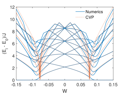
Figure 1: (Color Online) First fifteen energy-levels as a function of interspecies interaction $W$ for intraspecies interaction $U=0.01$ (energy units in $J$) and total boson number $N=60$ with $N_{a}=N_{b}$. The plots compare numerical results (continuous lines) with the analytical eigenvalues (dotted lines) computed within the CV method.

For twin boson populations $\epsilon_{a}=\epsilon_{b}$ so that $\epsilon=2/N^{2}$. This harmonic-oscillator Hamiltonian feature eigenvalues

$$E_{w}(n,m)=K+\sqrt{2\tau\epsilon^{2}(u+2\tau+w)}\Bigl{(}n+{1}/{2}\Bigr{)}$$

$$+\sqrt{2\tau\epsilon^{2}(u+2\tau-w)}\;\Bigl{(}m+1/2\Bigr{)}\;,$$ (13)

and the corresponding eigenstates are given by

$$\Psi_{n,m}(q,p)=\frac{e^{-\frac{1}{2}({q^{2}}/{\lambda^{2}}+{p^{2}}/{\nu^{2}})}}{\sqrt{\pi\lambda\nu\;2^{n+m}n!m!}}\;H_{n}\left(\frac{q}{\lambda}\right)H_{m}\left(\frac{p}{\nu}\right)$$ (14)

with $q=(x+y)/\sqrt{2}$, $p=(x-y)/\sqrt{2}$ and

$$\lambda^{2}=\sqrt{\frac{8\tau\epsilon^{2}}{w+u+2\tau}}\;,\quad\nu^{2}=\sqrt{\frac{8\tau\epsilon^{2}}{u-w+2\tau}}\,.$$

We note that the standard deviations $\lambda$ and $\nu$ controls the extension of the gaussian factors in $\Psi_{n,m}(q,p)$ and thus the degree of localization of this state in the Fock space described (within the CV method) by continuous variables $x$, $y$. The amplitude of the quadratic approximation of $V$ contained in (12) essentially corresponds, at the minimum point, to the gaussian curvature of $V$ which, in turn, is proportional to $1/(\nu\lambda)^{4}$.

The previous approximation is valid for weakly-excited states, namely, for energies relatively close to the ground-state energy. For the midspectrum states the CV approach is no longer valid in that the assumption of continuity on which relies may not hold cvp9 .

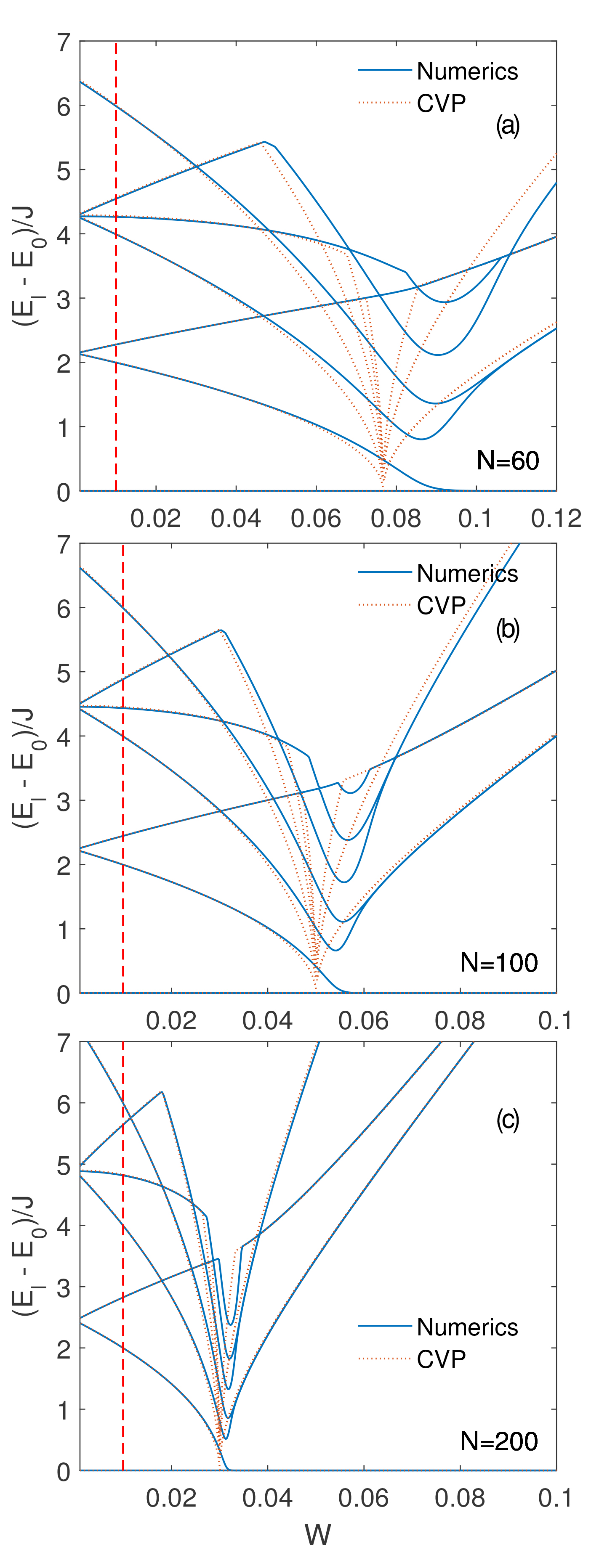
Figure 2: (Color Online) First seven energy-level as a function of interspecies interaction $W$ for $U=0.01$ (energy units in $J$) and boson number $N=60$ (panel (a)), $N=100$ (panel (b)) and $N=200$ (panel (c)). The plots compare numerical results (continuous lines) with the analytical eigenvalues computed within the CV method (dotted lines). The vertical dashed line at $W=0.01$ shows the critical value ($\omega=u+2\tau$) where the transition takes place in the thermodynamic limit.

Strong repulsive interaction $W$. For $w>u+2\tau$, the single minimum of potential $V$ splits into two symmetric minima at $x=\pm|x_{1}|$ and $y=\mp|x_{1}|$. One easily calculates the quadratic approximation of EH (5) in terms of the local-minima coordinates $\xi_{x}=x\pm|x_{1}|$ and $\xi_{y}=y\mp|x_{1}|$, in which the double sign is referred to the two symmetric minima of $V$. The further coordinate transformation $\xi_{x},\xi_{y}\to q,p$ where $q=(\xi_{x}+\xi_{y})/\sqrt{2}$ and $p=(\xi_{x}-\xi_{y})/\sqrt{2}$ leads to the diagonal, harmonic-oscillator form

$${\cal H}\simeq-\frac{4\tau^{2}\epsilon^{2}}{|w-u|}\;\Delta_{qp}+\left(\frac{u+w}{4}+\frac{(w-u)^{3}}{16\tau^{2}}\right)q^{2}$$

$$+\left(\frac{u-w}{4}+\frac{(w-u)^{3}}{16\tau^{2}}\right)p^{2}+u-\gamma-\frac{2\tau^{2}}{w-u}\;,$$ (15)

whose eigenvalues are given by

$$E_{s}(n,m)=\epsilon(w-u)\sqrt{1+\frac{4\tau^{2}(u+w)}{(w-u)^{3}}}\left(n+\frac{1}{2}\right)$$

$$+\epsilon\sqrt{(w-u)^{2}-4\tau^{2}}\left(m+\frac{1}{2}\right)+u-\gamma-\frac{2\tau^{2}}{w-u}\;.$$ (16)

The corresponding eigenstates have the form

$$\Phi_{n,m}(q,p)=\frac{e^{-\frac{1}{2}({q^{2}}/{\lambda^{2}}+{p^{2}}/{\nu^{2}})}}{\sqrt{\pi\lambda\nu\;2^{n+m}n!m!}}\;H_{n}\left(\frac{q}{\lambda}\right)H_{m}\left(\frac{p}{\nu}\right)$$ (17)

with $q=(x+y)/\sqrt{2}$, $p=(x-y\pm 2|x_{1}|)/\sqrt{2}$, where the term $\pm 2|x_{1}|$ bears memory of the two symmetric minima of the current case, and

$$\lambda^{2}=\frac{8\tau^{2}\epsilon}{\sqrt{(w-u)[4\tau^{2}(w+u)+(w-u)^{3}]}}\;,$$

$$\nu^{2}=\frac{8\tau^{2}\epsilon}{(w-u)\sqrt{(w-u)^{2}-4\tau^{2}}}\,.$$

As in the weak-interaction case, such an approximation holds for weakly-excited states and parameters $\nu$ and $\lambda$, related to the curvature of $V$, can be show to control the localization character of these states in the Fock space. State (17) actually corresponds to two independent states associated to the same eigenvalue $E_{s}(n,m)$ which we denote with

$$\Phi^{\pm}_{n,m}(x,y)=\Phi_{n,m}\left(\frac{x+y}{\sqrt{2}},\frac{x-y\pm|x_{1}|}{\sqrt{2}}\right)\;.$$ (18)

The latter describe the low-energy eigenfunctions localized in the neighborhood of the two minima of potential $V$. The degeneracy of the eigenvalues is a consequence of the partially-semiclassical character of the CV method. It can be removed by splitting each eigenvalue into a doublet $E^{\pm}_{s}(n,m)$ $=E_{s}(n,m)\pm\delta$, where the splitting $\delta$ is obtained through the procedure described in landau for the double-well potential. The simplest approximation of the eigenstates relevant to $E^{r}_{s}(n,m)$, $r=\pm$, is simply given by

$$\Psi^{r}_{n,m}(x,y)=\Bigl{(}\Phi^{+}_{n,m}+r\Phi^{-}_{n,m}\Bigr{)}/{\sqrt{2}}\;.$$ (19)

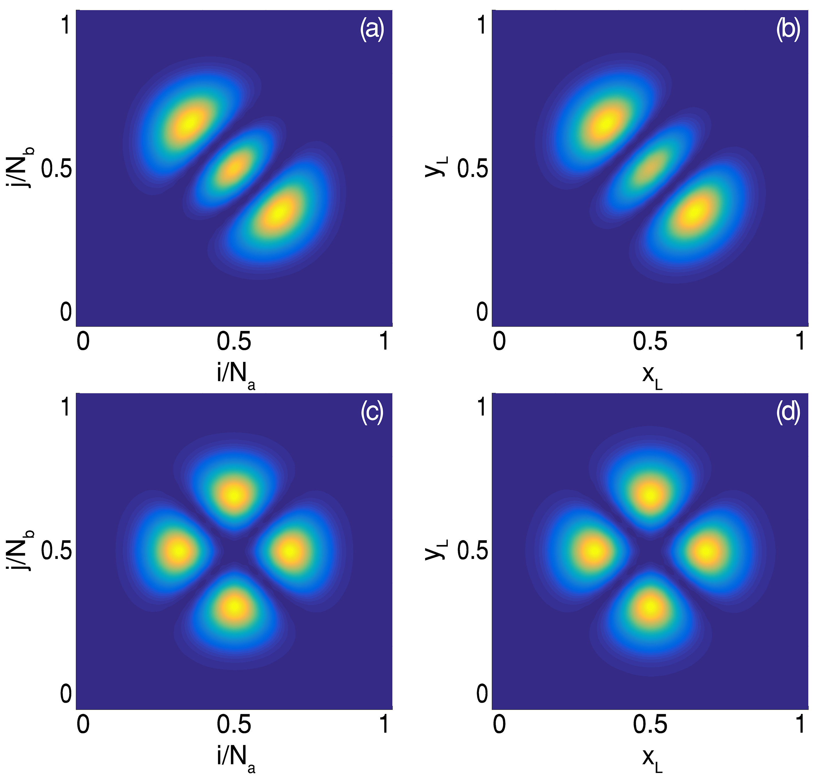
Figure 3: (Color Online) Excited-state probability amplitudes $|c_{ij}^{l}|^{2}$ calculated numerically (panels (a),(c)), compared with the probability densities $|\Psi_{n,m}|^{2}$ obtained by the CV method (panels (b),(d)). The upper (lower) row concerns the excited states $\Psi_{2,0}(q,p)$ ($\Psi_{1,1}(q,p)$) for the energy level $l=3$ ($l=4$) for $U/J=0.01$, $W/J=0.001$, and $N_{a}=N_{b}=30$. These correspond to two of the three eigenvalues $E_{l}$, $l=3,4,5$ forming the second plateau in Fig. 4.

Attractive interspecies interaction. In order to evidence the different features characterizing the model with an attractive interaction we report the eigenvalue spectra for $\omega<0$. These can be computed by following the same procedure of the repulsive case $\omega>0$ (the corresponding Hamiltonians are shown in Appendix B). For $|\omega|<u+2\tau$ (weak interaction) one finds

$$E_{w}^{\prime}(n,m)=K+\sqrt{2\tau\epsilon^{2}(u-|\omega|+2\tau)}\Big{(}n+\frac{1}{2}\Big{)}$$

$$+\sqrt{2\tau\epsilon^{2}(u+|\omega|+2\tau)}\Big{(}m+\frac{1}{2}\Big{)}$$ (20)

where one should remember that $K={(u+\omega)}/{2}-2\tau-\gamma$ and $\gamma=UN/2$ in the twin-component case. For $|\omega|>u+2\tau$ (strong interaction)

$$E_{s}^{\prime}(n,m)=\epsilon(|\omega|-u)\sqrt{1+\frac{4\tau^{2}(|\omega|+u)}{(|\omega|-u)^{3}}}\Big{(}m+\frac{1}{2}\Big{)}$$

$$+\epsilon\sqrt{(|\omega|-u)^{2}-4\tau^{2}}\Big{(}n+\frac{1}{2}\Big{)}+u-|\omega|-\frac{2\tau^{2}}{|\omega|-u}-\gamma.$$ (21)

Figure 1 well illustrates the perfect symmetry characterizing the energy spectrum when the interspecies interaction $w$ changes from positive (repulsive case) to negative (attractive case). This figure (and the subsequent ones) show the dependence of $(E_{\ell}-E_{0})/J$ on $W/J$. Index $\ell$ in $E_{\ell}$ orders eigenvalues (13), (16), (20), and (21), according to their increasing values. The reason for considering $E_{\ell}-E_{0}$ is that the eigenvalues $E_{\ell}$, $\ell\geq 0$ obtained with the CV method exhibit a finite shift with respect to the numerical eigenvalues. This deviation is a typical artifact of the quantization schemes including a semiclassical approximation gutz . In the present case the deviations $E^{ap}_{\ell}-E^{ex}_{\ell}$ between approximate and exact eigenstates can be shown to be proportional to $1/N^{2}$ ($1/N$) in the weak (strong) interaction regime and thus to be negligible for $N$ large enough.

Figure 1 compares the exact spectrum with the spectrum obtained through the CV method for a total boson number $N=60$ and $N_{a}=N_{b}$. The critical points of the repulsive and attractive cases are situated at $W/J\simeq+0.076$ and $W/J\simeq-0.076$, respectively. At these values, both $E_{w}(n,m)$, $E_{s}(n,m)$ and $E_{w}^{\prime}(n,m)$, $E_{s}^{\prime}(n,m)$ tend to zero (see the dotted orange plots), while, in their proximity, the exact eigenvalues (blue continuous plots) exhibit a significant decrease culminating in a minumum. Due to the relatively small value of $N$, the agreement between the exact an the approximate spectrum appears only at a sufficient distance from the critical points, but improves when $N$ is increased. This case is discussed in the next section where, owing to the spectrum symmetry, we focus on the case $W/J\geq 0$.

V Discussion

We analyze the limit $w\to(u+2\tau)^{\pm}$. In this case, it is straightforward to check that the Hamiltonians (12) and (15) collapse into a unique one

$${\cal H}_{S}={\cal H}_{W}\simeq\,\left(u-\tau\right)-2\tau\epsilon^{2}\left(\frac{\partial^{2}}{\partial q^{2}}+\frac{\partial^{2}}{\partial p^{2}}\right)+\frac{u+2\tau}{4}q^{2}\;,$$

in which the $p^{2}$-dependent terms go to zero due to the vanishing of the frequencies $\sqrt{2\tau\epsilon^{2}(u+2\tau-w)}$ in (12), and $\sqrt{(u-w)^{2}-4\tau^{2}}$ in (15). This effect causes in the eigenvalues (13) and (16) the spectral collapse, namely, the vanishing of the interlevel distance relevant to the quantum number $m$ as shown by

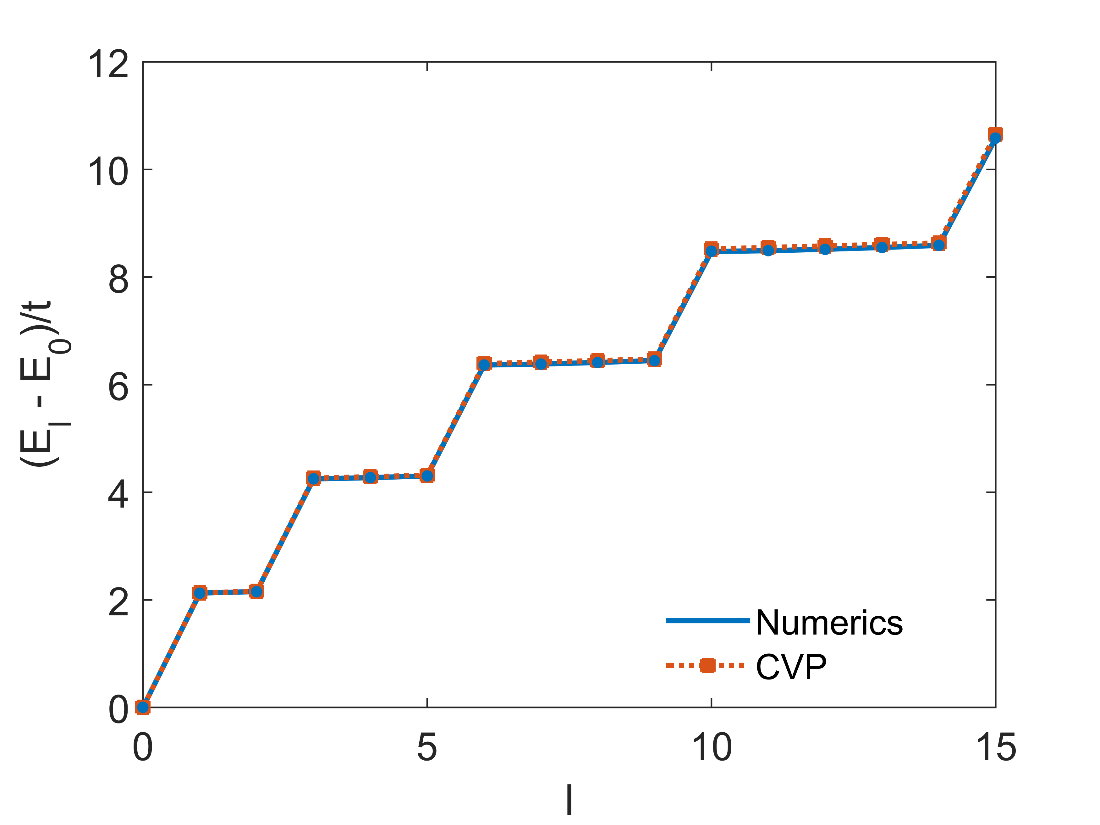
Figure 4: (Color Online) Energy levels for $U/J=0.01$, $W/J=0.001$, $N_{a}=N_{b}=30$, calculated numerically (continuous blue line) and within the CV picture (CVP). The apparent formation of groups of degenerate eigenvalues (plateaux) is commented in the text.

$$E_{w}(n,m)=E_{s}(n,m)\simeq u-\gamma-\tau+\epsilon\sqrt{\tau(u+2\tau)}\left(2n+1\right)$$

$$+\epsilon\sqrt{\tau|w-u-2\tau|}\left(2m+1\right)$$ (22)

for $w-u-2\tau\to 0$. When $w$ reachs the critical point $w\equiv u+2\tau$, the free-particle term $-2\tau\epsilon^{2}{\partial^{2}_{p}}$ in the Hamiltonian entails the spectrum

$$E(n,k)=u-\tau-\gamma+2\sqrt{\tau\epsilon^{2}(u+2\tau)}\left(n+\frac{1}{2}\right)+2\tau\epsilon^{2}k,$$

in which the contribution of quantum number $m$ is replaced by the $k$-dependent term, while in

$$\Phi_{n,k}(q,p)\propto e^{-{q^{2}}/{(2\lambda^{2}})}H_{n}\left({q}/{\lambda}\right)e^{ikp}\;$$

the $p$-dependent gaussian becomes a plane wave. The progressive reduction of the interlevel distance (culminating, at the critical point, with the transition of the $m$-dependent energy band to a continuous energy distribution) then represents the distinctive trait marking the emergence of a ground state with a different structure. It is worth recalling that, this change consists in the transition from a ground state with two bosonic components totally mixed and delocalized ($w<u+2\tau$) to a ground state whose components are completely localized ($w>u+2\tau$). The exact spectrum, determined by means of numerical simulations, confirms the validity of the scenario emerging from the CV method as soon as the boson numbers is sufficiently increased.

Figure 2 describes the first seven energy levels as a function of interspecies interaction $W/J$ for total boson numbers $N=60,100,200$. The plots compare the eigenvalues obtained numerically with the eigenvalues computed analytically by means of the CV method.

At the critical point $W/J=$ $U/J+4/N$ (derived from $w=u+2\tau$ thanks to the definitions (4) and populations $N_{a}=N_{b}=N/2$) all the eigenvalues determined with the CV method continuously drop to zero. The vertical dashed line corresponds to the critical value of the interspecies interaction $W$ one finds in the thermodynamic limit $N\to\infty$ and with $U=0.01J$ (energy units in $J$). In this limit one has $W=U$, reproducing the well-known critical value at which, for $W$ repulsive, the two components separate pra92 .

Figure 2 clearly shows how, by increasing $N$, the exact eigenvalues more and more tend to reproduce the critical behavior predicted by the CV method, while the critical value of $W/J$ approaches its limiting value 0.01. We observe, however, that even for $N=60$ the agreement between exact and CV-picture (CVP) spectrum becomes good right outside the neighborhood of the critical point.

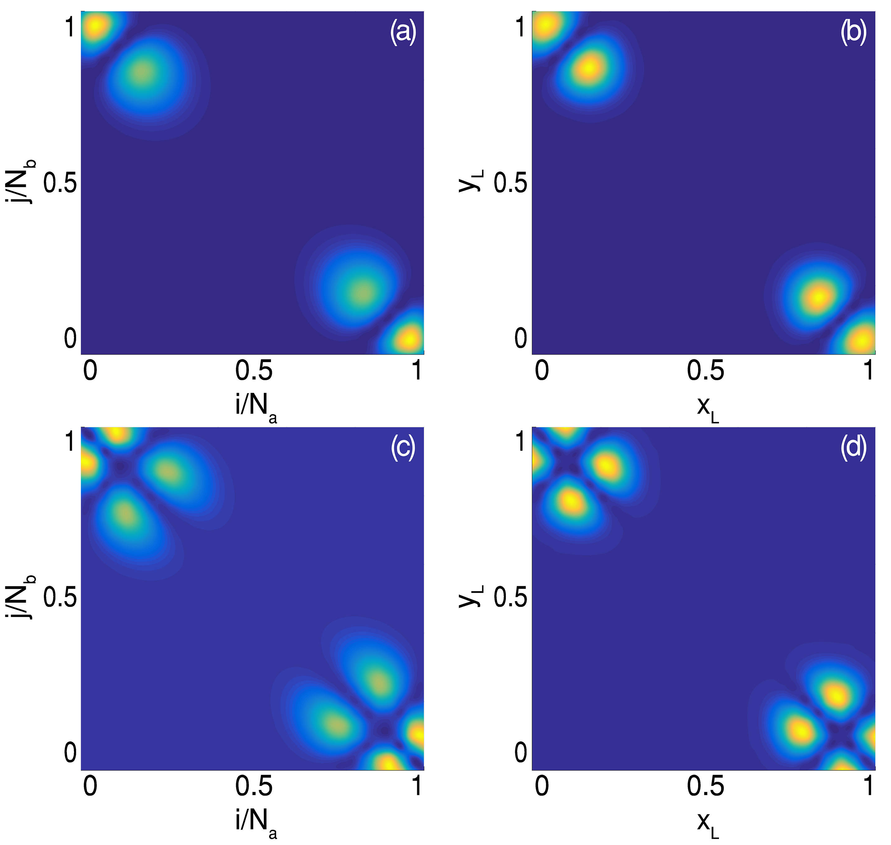
Figure 5: (Color Online) Excited-state probability amplitudes $|c_{ij}^{l}|^{2}$ calculated numerically (panels (a),(c)), compared with the probability densities $|\Psi^{+}_{n,m}|^{2}$ obtained by the CV method (panels (b),(d)). The upper (lower) row concerns the excited states $\Psi^{+}_{0,1}(x,y)$ ($\Psi^{+}_{0,2}(x,y)$) for the energy level $l=2$ ($l=8$) for $U/J=0.01$, $W/J=0.12$, and $N_{a}=N_{b}=30$. These correspond to the eigenvalues $E_{2}=E_{s}(0,1)$ (second plateau), and $E_{8}=E_{s}(1,1)$ (fifth plateau) in Fig. 6.

V.1 Weakly-excited states

We complete the comparison of the exact (numerical) scheme with the CV method by considering the exact eigenstates and their CVP counterparts described by formulas (14) and (19). The latter allow the reconstruction of the approximate eigenstates

$$|\Psi_{E}\rangle=\sum_{{\vec{x}},{\vec{y}}}\psi_{E}({\vec{x}},{\vec{y}})|x_{R},x_{L},y_{R},y_{L}\rangle$$

according with formula (3), where the amplitude $\psi_{E}({\vec{x}},{\vec{y}})$ identifies with $\Psi_{nm}(q,p)$ or $\Psi^{\pm}_{nm}(x,y)$ (see formulas (14) and (19)) when $x_{R}$, $x_{L}$, $y_{R}$, $y_{L}$ are expressed in terms of variables $q$, $p$ (or $x$, $y$), and states $|x_{R},x_{L},y_{R},y_{L}\rangle$ are the continuous form of Fock states $|n_{R},n_{L},m_{R},m_{L}\rangle$.

Figure 3 illustrates the structure of some eigenstates in the weak-interaction regime $U/J=0.01$, $W/J=0.001$. The probabilities $|c_{ij}|^{2}$ obtained from the exact eigenstates $|E\rangle=\sum_{i}\sum_{j}c_{ij}(E)|N_{a}-i,i,N_{b}-j,j\rangle$ are compared with their CVP counterparts $|\psi_{n,m}|^{2}$, where the amplitudes are $\psi_{n,m}(x_{L},y_{L})=$ $\Psi_{n,m}(q,p)$ and $p=$ $\sqrt{2}(x_{L}-y_{L})$, $q=$ $\sqrt{2}(x_{L}+y_{L}-1)$. One should remember that only two of the four coordinates $x_{\alpha}$, $y_{\alpha}$ are independent due to the constraints $x_{R}+x_{L}=1$, $y_{R}+y_{L}=1$.

In Figure 3, the probability density of the eigenstates associated to the three eigenvalues forming the second plateau of Fig. 4 are represented. In Figure 3 and in the subsequent ones, dark blue stands for a vanishing probability density while bright yellow denotes its relative maxima. Note that the presence of the energy plateaux shown in Fig. 4 is only apparent: The groups of quasidegenerate eigenvalues with $E_{l}\simeq constant$ for $n+m=0,1,2,...$ are the consequence of the parameter choice $U/J=0.01$$=10\;W/J$ making the two harmonic-oscillator frequencies in (13) almost equal.

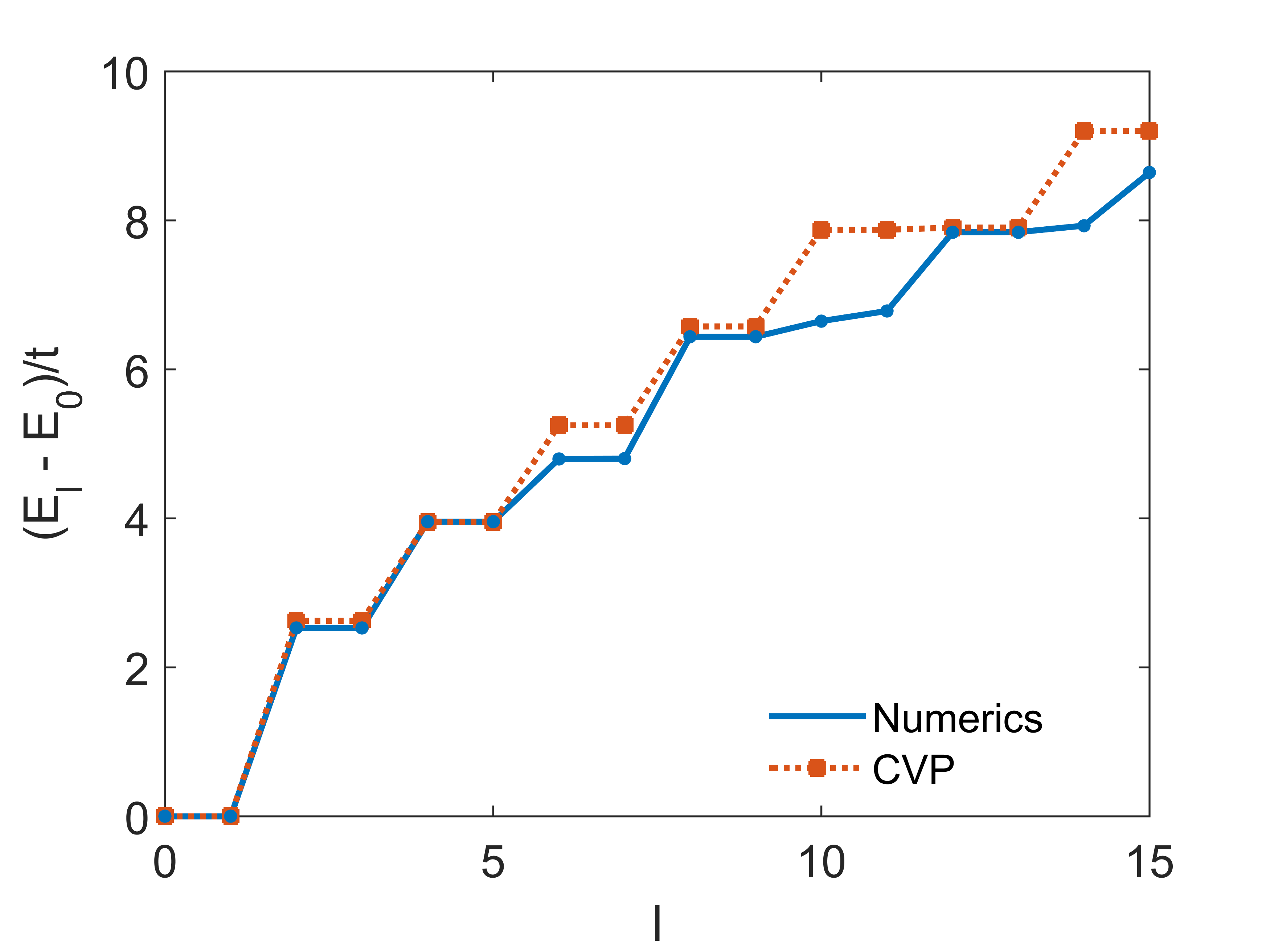
Figure 6: (Color Online) Energy levels for $U/J=0.01$, $W/J=0.001$, $N_{a}=N_{b}=30$, calculated numerically (continuous blue line) and within the CVP (orange dotted line). The apparent formation of groups of degenerate exact eigenvalues (plateaux) is commented in the text.

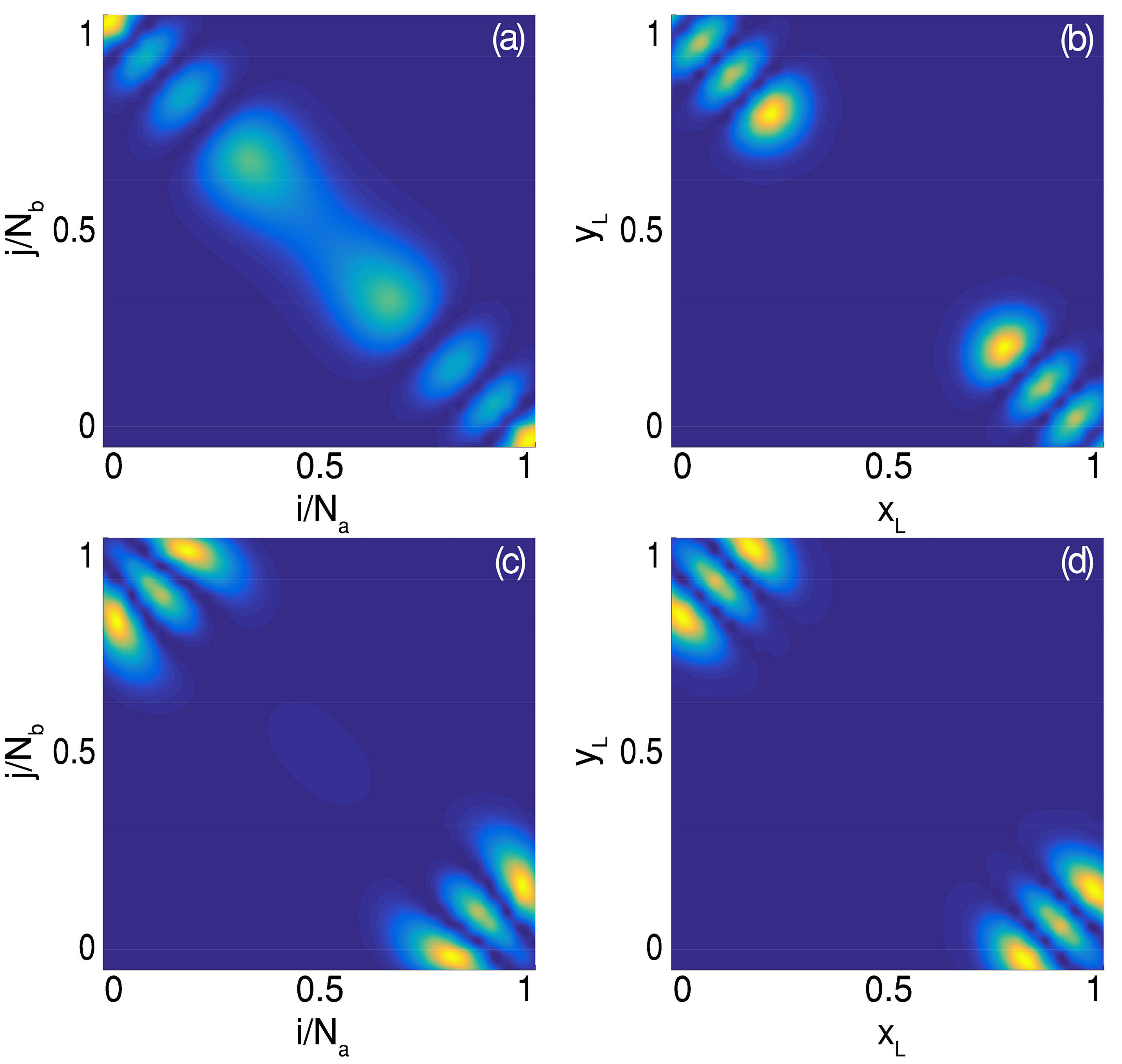
Figure 7: (Color Online) Excited-state probability amplitudes $|c_{ij}^{l}|^{2}$ calculated numerically (panels (a),(c)), compared with the probability densities $|\Psi^{+}_{n,m}|^{2}$ obtained by the CV method (panels (b),(d)). The upper (lower) row concerns the excited states $\Psi^{+}_{2,0}(x,y)$ ($\Psi^{+}_{0,3}(x,y)$) for the energy level $l=10$ ($l=12$) for $U/J=0.01$, $W/J=0.12$, and $N_{a}=N_{b}=30$. These correspond to the eigenvalues $E_{10}=E_{s}(2,0)$ and $E_{12}=E_{s}(0,3)$ in Fig. 6.

Figure 3 displays the probability density of the eigenfunctions $\Psi_{2,0}(q,p)$ and $\Psi_{1,1}(q,p)$, which feature three and four peaks, respectively. The state $\Psi_{0,2}(q,p)$ exhibits the same probability distribution (not shown) as $\Psi_{2,0}(q,p)$ but the three peaks are placed along the second diagonal of the box. This figure clearly shows how the exact and CVP probability densities are almost indistinguishable, a result further confirmed by other choices of $n$ and $m$. Therefore the exact scheme and the CVP exhibit an excellent agreement.

Figure 5 displays the probability density of some eigenstates in the strong-interaction regime with $U/J=0.01$, $W/J=0.12$. As in the weak-interaction case we compare the $|c_{ij}|^{2}$ with the CVP probabilities $|\psi_{n,m}|^{2}$, but in this regime $\psi_{n,m}(x_{L},y_{L})=$ $\Psi^{\pm}_{n,m}(x,y)$, the eigenfunctions (19) of energies $E_{s}(n,m)$. Coordinates $x$ and $y$ are linear functions of $x_{L}$, $y_{L}$. Figure 5 compares the probability density for the excited states $\Psi^{+}_{01}(x,y)$ and $\Psi^{+}_{02}(x,y)$ (with energies $E_{s}(0,1)$ and $E_{s}(0,2)$, respectively) obtained in the CVP with those found in the exact scheme. These confirm the remarkable agreement of the CVP with numerical results.

The corresponding energy eigenvalues are illustrated in Figure 6. The CVP eigenvalues are, by construction, degenerate and form the doublets $E_{2l}=E_{2l+1}$ (orange dots). The link with energies (16) is given by $E_{0}=E_{s}(0,0)$, $E_{2}=E_{s}(0,1)$, $E_{4}=E_{s}(1,0)$, $E_{6}=E_{s}(0,2)$, $E_{8}=E_{s}(1,1)$ … listed in increasing order. It is worth remembering that this degeneracy is inherent in the CV method (see the discussion before eq. (19)), whereas the degeneracy of some exact eigenvalue is only apparent.

The important point concerning Fig. 6 is that at least ten CVP eigenvalues exhibit an excellent agreement with their numerical counterparts. Visible deviations appear in an intermittent way along the eigenvalue sequence (see, for example, $E_{6}$, $E_{7}$, and $E_{10}$, $E_{11}$) but they remain relatively small with respect to the trend of the the overall sequence. The increase of boson number $N$ can be shown to reduces this effect.

Figure 7 (upper panels) aims to illustrate the differences affecting the exact probability distribution and the CVP distribution for $\Psi^{+}_{20}(x,y)$, a state whose eigenvalue $E_{10}=E_{s}(2,0)$ deviates from its numerical counterpart. Even if, in general, their overall structure is not too different, the upper left panel features two internal peaks exhibiting a weak separation, whereas, in the upper right panel, these peaks are completely separated. Moreover, the left panel shows two major peaks (at the corners of the box) which are almost negligible in the right panel. The two probability densities again, almost perfectly, match to each other when considering the (non deviating) eigenvalue $E_{12}=E_{s}(0,3)$ relevant to the eigenstate $\Psi^{+}_{03}(x,y)$.

We conclude by showing in Figure 8 the sequence illustrating the probability densities of the ground state when $W/J$ ranges from the weak to the strong interaction regime (up-to-bottom). For $W/J=0.001$ a unique central peaks appears at $x_{L}=y_{L}=0.5$ ($\to x_{R}=y_{R}=0.5$) meaning that the configuration with the maximum probability is that where the two components are equally distributed in the two wells. The boson populations are mixed and delocalized. For $W/J=0.170$, the two peaks emerging from the transition implies that $x_{L}\simeq 0$, $y_{L}\simeq 1$ and $x_{R}\simeq 10$, $y_{R}\simeq 0$, namely, the two component are fully separated. The agreement of numerical results and CVP predictions is quite satifactory.

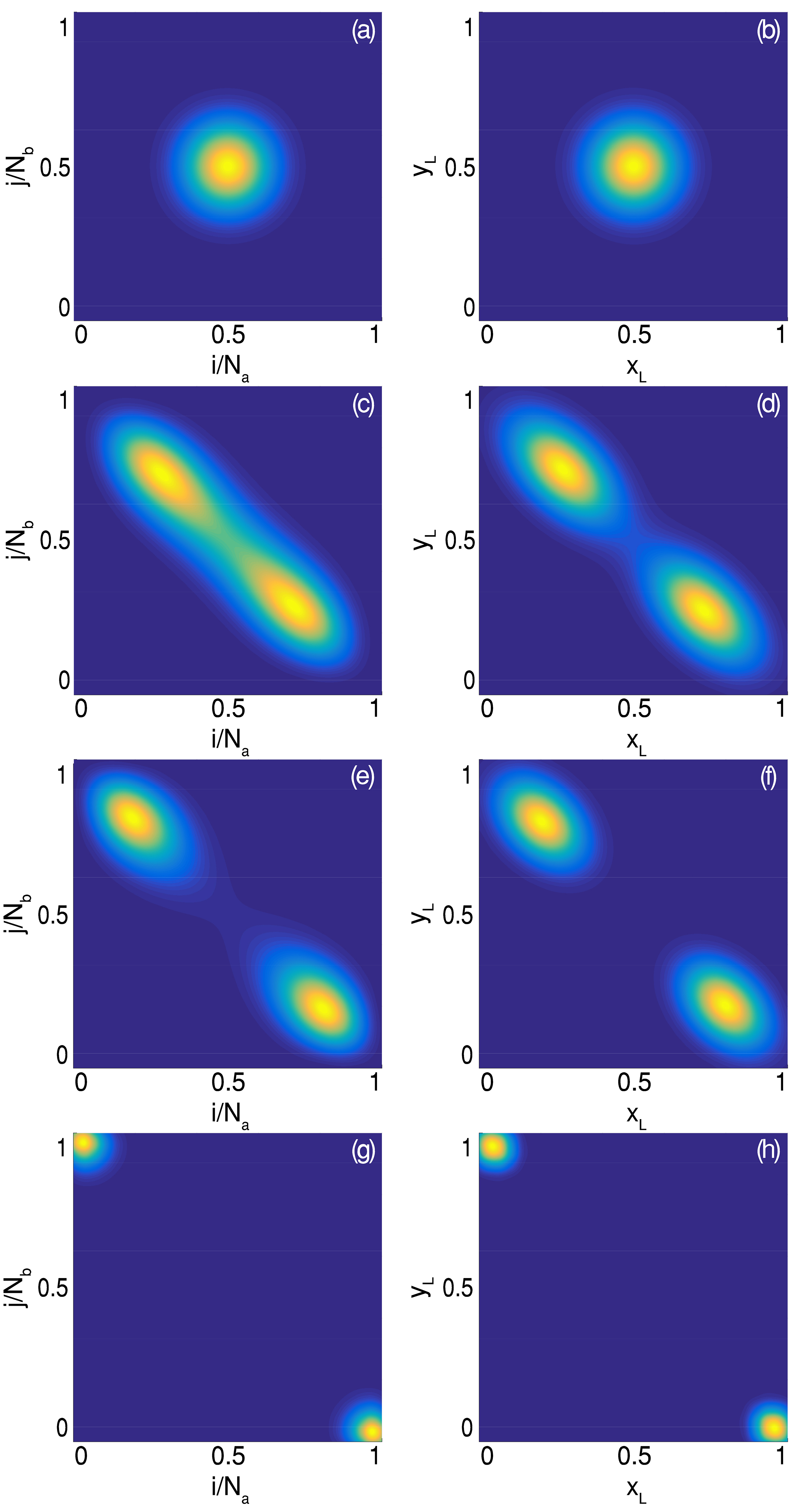
Figure 8: (Color Online) Probability densities of the ground state for $U/J=0.01$, $N_{a}=N_{b}=30$, and (from top to bottom) $W/J=0.001,0.085,0.093,0.170$. Right column: probability density obtained from states (14) and (19) with $m=n=0$, within the CV method. Left column: probability amplitudes $|c_{ij}^{0}|^{2}$ for the exact ground state calculated numerically.

VI Conclusions

We have studied the effectiveness of the CV method by applying this scheme to the BH-like Hamiltonian describing a bosonic gas with two components trapped in a double-well potential. As it is well known, this system exhibits a macroscopic dynamical phase transition to states with localized populations when the effective interaction $W/U$ is large enough. The presence of this transition plays an important role in our analysis since it makes the application of the CV method more demanding and thus more significant. We have analyzed the low energy spectrum and its eigenstates by considering both the repulsive and the attractive regime of $W$.

After reformulating, in Section II, the TDH within the continuous-variable picture, we have calculated the energy eigenvalues and the corresponding eigenstates in Section III. In this Section, we have also showed that the reduction of the interlevel distance predicted by the CV method close to the transition point is confirmed by numerical simulations. These also succeed in reproducing the spectral collapse for number of bosons sufficiently large, a condition which well fits the basic assumption of the CV method that the local population fractions $n_{i}/N$ are almost continuous.

To further check the effectiveness of the CV method we have compared both the weakly excited states and the corresponding energy levels derived within the CV method with those determined numerically. While in the weak interaction regime the agreement is excellent, in the strong interaction regime some eigenvalues exhibit visible but limited deviations from their numerical counterparts. Such deviations appear in an intermittent way in correspondence to sufficiently excited states and, rather reasonably, seem to be related to the intrinsic degeneracy of the CVP eigenvalues when the minimum of the potential splits into two separated minima.

The agreement is again considerably good when comparing the probability density of the exact and the CVP ground state both in the weak and in the strong interaction regime. In general, the CVP eigenstates closely mimic the exact eigenstates whenever a numerical eigenvalue well matches the CVP eigenvalue.

The previous analysis indeed suggests that the CV method provides an effective approach for describing the energy spectrum and the eigenstates of multimode bosonic systems. The discrepancies which partially affect the spectrum in certain regimes seem to have negliglible effects on the critical behavior leading to the spectral collapse provided that a large number of bosons is involved. This is confirmed as well by the successful application of the CV method for detecting the critical properties of the self-trapping transition in the attractive BH trimer cvp9 . The great feasibility of this method within multimode bosonic systems promises a wide range of applications in the field of atomic currents atom1 -atom3 and more in general of atomtronics devices atom4 , atom5 .

Concluding, the effects discussed in this paper should be accessible to experimental observations by confining mixtures in a double-well trap. As is well known, the semiclassical dynamics of a single-component condensate has been successfully investigated in a double-well device realized by albiez , anker , and has shown the nonlinear oscillations predicted by the theory and the inherent self-trapping phenomenon. As in the single-component case, the double-well geometry should be realized by superposing the (sinusoidal) linear potential confining mixtures lens , gadway in optical lattices with a parabolic trap of controllabe amplitude. Further develpments in the dynamics of mixtures in multiwell systems are expected from the realization of the ring geometry designed in atom3 .

Appendix A Semiclassical form of the TDH

The derivation of the semiclassical TDH can be performed by means of the coherent-state variational method where operators become classical variables within a sort of generalized Bogoliubov scheme sc1 . The semiclassical Hamiltonian associated to (1) is easily found to be

$$H_{s}=H_{a}+H_{b}+W(|\alpha_{L}|^{2}|\beta_{L}|^{2}+|\alpha_{R}|^{2}|\beta_{R}|^{2}),$$

where $H_{a}=-J_{a}(\alpha^{*}_{L}\alpha_{R}+C.C.)+U_{a}\sum_{r}|\alpha_{r}|^{4}/2$ and $H_{b}$ has the same form with $\beta_{r}$ ($J_{b}$ and $U_{b}$) in place of $\alpha_{r}$ ($J_{a}$ and $U_{a}$). The classical quantities $N_{a}=|\alpha_{L}|^{2}+|\alpha_{R}|^{2}$ and $N_{b}=|\beta_{L}|^{2}+|\beta_{R}|^{2}$ can be shown to be conserved quantities as in the quantum picture. By using the classical version $x=(|\alpha_{L}|^{2}-|\alpha_{R}|^{2})/N_{a}$ and $y=(|\beta_{L}|^{2}+|\beta_{R}|^{2})/N_{b}$ of the operators leading to the EH (5), one obtains, up to a constant term,

$${H}_{s}=\frac{u_{a}}{4}\Bigl{(}1+x^{2}\Bigr{)}+\frac{u_{b}}{4}\Bigl{(}1+y^{2}\Bigr{)}+\frac{w}{2}(1+xy)$$

$$-\Bigl{(}\tau_{a}{\sqrt{1-x^{2}}}\cos(2\theta_{x})+\tau_{b}{\sqrt{1-y^{2}}}\cos(2\theta_{y})\Bigr{)}\;,$$ (23)

where $\theta_{x}=(\phi_{L}-\phi_{R})/2$, $\theta_{y}=(\nu_{L}-\nu_{R})/2$ are angle variables canonically conjugate with the action variables $x$ and $y$ satisfying the Poisson Brackets $\{x,\theta_{x}\}=1/(\hbar N_{a})$, $\{y,\theta_{y}\}=1/(\hbar N_{b})$. Variables $\phi_{r}$ ($\nu_{r}$) are the phases of the local order parameters $\alpha_{r}=|\alpha_{r}|e^{i\phi_{r}}$ ($\beta_{r}=|\beta_{r}|e^{i\nu_{r}}$). The Poisson brackets of $|\alpha_{r}|^{2}$, $|\beta_{r}|^{2}$ with $\phi_{r}$, $\nu_{r}$ can be easily evinced from the canonical ones $\{\alpha_{r},\alpha^{*}_{r}\}=1/(i\hbar)$, $\{\beta_{r},\beta^{*}_{r}\}=1/(i\hbar)$ supplied by the coherent-state variational method and reminescent of the boson mode commutators. $[a_{r},a^{+}_{r}]=1$, $[b_{r},b^{+}_{r}]=1$.

Appendix B Quadratic approximation of $V$ for $w<0$

We perform the quadratic approximation of $V$ in the proximity of its local minima, focusing on the attractive case (the same scheme holds in the repulsive case). The minimum coordinates are given by

$$x_{0}^{\prime}=y_{0}^{\prime}=0,\;\;\;\;x_{1}^{\prime}=\pm\sqrt{1-{4\tau^{2}}/{(|\omega|-u)^{2}}}\;.$$ (24)

By expanding potential $V$ in the proximity of its minima one finds that points $x_{0}^{\prime}=y_{0}^{\prime}=0$ and $x_{1}^{\prime}=y_{1}^{\prime}$ describe the minimum-energy configuration in the regimes $|\omega|<u+2\tau$ and $|\omega|>u+2\tau$ respectively.

In the attractive case $\omega<0$, the EH is $\mathcal{H}=V-D$, where $D$ has the same form as in (5), and

$$V=-\gamma+\frac{u}{4}\Big{(}1+x^{2}\Big{)}+\frac{u}{4}\Big{(}1+y^{2}\Big{)}$$

$$-\frac{|\omega|}{2}\Big{(}1+xy\Big{)}-\tau\Big{(}\sqrt{1+x^{2}}+\sqrt{1+y^{2}}\Big{)}\;,$$ (25)

where $\gamma=UN/2$. Potential $V$ is represented around the potential minima by means of its Taylor expansion. The resulting quadratic form is written in terms of local coordinates $\xi_{x}=(x-\bar{x})$ and $\xi_{y}=(y-\bar{y})$ and $\bar{x}$, $\bar{y}$.

Weak interspecies interaction. For $|\omega|<u+2\tau$, the minimum coordinates are $\bar{x}=x_{0}^{\prime}=0$ and $\bar{y}=y_{0}^{\prime}=0$. In this case

$$\partial_{x}^{2}V=\partial_{y}^{2}V=\frac{u}{2}+\tau\;,\quad\partial_{y}\partial_{x}V=-\frac{|\omega|}{2}\;.$$

Setting $\xi_{x}=(q+p)/\sqrt{2}$ and $\xi_{y}=(q-p)/\sqrt{2}$ the EH becomes ${\cal H}=-2\tau\epsilon^{2}(\partial^{2}_{q}+\partial^{2}_{p})+V$ where the expanded potential reads

$$V=K^{\prime}+\frac{u-|\omega|+2\tau}{4}q^{2}+\frac{u+|\omega|+2\tau}{4}p^{2}$$

with $K^{\prime}=({u-|\omega|-4\tau}-{UN})/{2}$. Then the eigenvalues of the two independent harmonic oscillators occurring in $\cal H$ can be easily computed. One finds

$$E_{W}(n,m)=K^{\prime}+\sqrt{2\tau\epsilon^{2}(u-|\omega|+2\tau)}\Big{(}n+\frac{1}{2}\Big{)}$$

$$+\sqrt{2\tau\epsilon^{2}(u+|\omega|+2\tau)}\Big{(}m+\frac{1}{2}\Big{)}$$ (26)

Strong interspecies interaction. For $|\omega|>u+2\tau$, the coordinates of the potential minimum are $\bar{x}=x_{1}^{\prime}$ and $\bar{y}=y_{1}^{\prime}$. In this case

$$\partial_{x}^{2}V=\frac{u}{2}+\frac{\tau}{(1-x^{2})^{\frac{3}{2}}}\;,\,\,\,\partial_{y}^{2}V=\frac{u}{2}+\frac{\tau}{(1-y^{2})^{\frac{3}{2}}}\;$$

and $\partial_{x}\partial_{y}V=-{|\omega|}/{2}$. By setting $\xi_{x}=(q+p)/\sqrt{2}$ and $\xi_{y}=(q-p)/\sqrt{2}$, the expanded potential reduces to

$$V(q,p)=K^{\prime\prime}+\frac{w_{q}^{2}}{2}\;q^{2}+\frac{w_{p}^{2}}{2}\;p^{2}$$ (27)

with

$$w^{2}_{q}=\frac{u-|\omega|}{2}+\frac{(|\omega|-u)^{3}}{8\tau^{2}}\;,\,w^{2}_{p}=\frac{u+|\omega|}{2}+\frac{(|\omega|-u)^{3}}{8\tau^{2}},$$

and $K^{\prime\prime}=({u-|\omega|-4\tau}-{UN})/{2}$, while the Hamiltonian of the system takes the form

$$\mathcal{H}=V_{1}^{\prime}-\frac{4\tau^{2}\epsilon^{2}}{||w|-u|}\Big{(}{\partial_{q}^{2}}+{\partial_{p}^{2}}\Big{)}+\frac{w_{q}^{2}}{2}\;q^{2}+\frac{w_{p}^{2}}{2}\;p^{2}$$ (28)

with $V_{1}^{\prime}\equiv V(x_{1}^{\prime},y_{1}^{\prime})=u-|\omega|-{2\tau^{2}}/{(|\omega|-u)}-{UN}/{2}$. Then the eigenvalues can be easily computed by considering the two independent harmonic-oscillator problems related to the coordinates $p$ and $q$, respectively.

$$E_{S}(n,m)=V_{1}^{\prime}+\epsilon(|\omega|-u)\sqrt{1-\frac{4\tau^{2}}{(|\omega|-u)^{2}}}\Big{(}n+\frac{1}{2}\Big{)}$$

$$+\epsilon(|\omega|-u)\sqrt{1+\frac{4\tau^{2}(|\omega|+u)}{(|\omega|-u)^{3}}}\Big{(}m+\frac{1}{2}\Big{)}\,.$$ (29)

References

- (1) L. Cruzeiro-Hansson, H. Feddersen, R. Flesch, P. L. Christiansen, M. Salerno, and A. C. Scott, Phys. Rev. B 42, 522 (1990).
- (2) E. Wright, J. C. Eilbeck, M. H. Hays, P. D. Miller, and A. C. Scott, Physica D 69, 18 (1993).
- (3) S. Flach and V. Fleurov, J. Phys.: Condens. Matter 9, 7039 (1997).
- (4) A. Polkovnikov, S. Sachdev, and S. M. Girvin, Phys. Rev. A 66, 053607 (2002)
- (5) P. Buonsante, V. Penna, and A,. Vezzani, Phys. Rev. A 72, 043620 (2005).
- (6) A. R. Kolovsky, H. J. Korsch, and E. M. Graefe, Phys. Rev. A 80, 023617 (2009).
- (7) P. Buonsante, R. Franzosi and V. Penna, J. Phys. A 42, 285307 (2009).
- (8) P. Buonsante, V. Penna, A. Vezzani, Phys. Rev. A 82, 043615 (2010).
- (9) G. Mazzarella, L. Salasnich, A. Parola, and F. Toigo, Phys. Rev. A 83 053607 (2011).
- (10) H. Hennig, D. Witthaut, and D. K. Campbell, Phys. Rev. A 86 051604(R) (2012).
- (11) P. J. Jason and M. Johansson, Phys. Rev. A 86, 016214 (2012).
- (12) Xizhi Han and Biao Wu, Phys. Rev. A 93, 023621 (2016).
- (13) P. J. Jason and M. Johansson, Phys. Rev. E 94, 052215 (2016).
- (14) L. Amico and V. Penna, Phys. Rev. Lett. 80, 2189 (1998).
- (15) A. M. Rey, K. Burnett, R. Roth, M. Edwards, C. J. Williams and C. W. Clark, J. Phys. B: At. Mol. Opt. Phys. 36, 825 (2003).
- (16) J. Zakrzewski, Phys. Rev. A 71, 043601 (2005).
- (17) R. W. Spekkens and J. E. Sipe, Phys. Rev. A 59, 3868 (1999).
- (18) R. Franzosi and V. Penna, Phys. Rev. A 63, 043609 (2001)
- (19) T.-L. Ho, C. V. Ciobanu, J. Low Temp. Phys. 135, 257 (2004).
- (20) P. Zin, J. Chwedenczuk, B. Oles, K. Sacha, and M. Trippenbach, Europhys. Letters 83, 64007 (2008).
- (21) P. Buonsante, R. Burioni, E. Vescovi, and A. Vezzani, Phys. Rev. A 85, 043625 (2012).
- (22) V. S. Shchesnovich and V. V. Konotop, Phys. Rev. A 75, 063628 (2007).
- (23) J. Javanainen, Phys. Rev. A 60, 4902 (1999).
- (24) P. Buonsante, V. Penna, A. Vezzani, Phys. Rev. A 84, 061601(R) (2011).
- (25) G. Mazzarella, and V. Penna, J. Phys. B: At. Mol. Opt. Phys. 48, 065001 (2015).
- (26) C. Emary and T. Brandes, Phys. Rev. E 67, 066203 (2003).
- (27) S. Felicetti, J. S. Pedernales, I. L. Egusquiza, G. Romero, L. Lamata, D. Braak, and E. Solano, Phys. Rev. A 92, 033817 (2015)
- (28) V. Penna and F. A. Raffa, Int. J. Quantum Inform. 12, 1560010 (2014).
- (29) V. Penna, Phys. Rev. E 87, 052909 (2013).
- (30) F. Lingua, G. Mazzarella, and V. Penna, J. Phys. B 49, 205005 (2016).
- (31) X. Q. Xu, L. H. Lu, and Y. Q. Li, Phys. Rev. A 78 (2008) 043609
- (32) I. I. Satija, R. Balakrishnan, P. Naudus, J. Heward, M. Edwards and C. W. Clark, Phys. Rev. A 79 (2009) 033616
- (33) B. Juliá-Díaz, M. Melé-Messeguer, M. Guilleumas and A. Polls, Phys. Rev. A 80 (2009) 043622
- (34) G. Mazzarella, B. Malomed, L. Salasnich, M. Salerno and F. Toigo, J. Phys. B: At. Mol. Opt. Phys. 44 (2011) 035301
- (35) A. Naddeo and R. Citro, J. Phys. B: At. Mol. Opt. Phys. 43 (2010) 135302
- (36) P. Mujal, B. Julía-Díaz, and A. Polls, Phys. Rev. A 93, 043619 (2016)
- (37) B. B. Baizakov, A. Bouketir, A. Messikh, and B. A. Umarov, Phys. Rev. E 79 (2009) 046605
- (38) J.-S. Huang, Z.-W. Xie, M. Zhang and L.-F. Wei, J. Phys. B: At. Mol. Opt. Phys. 43 (2010) 065305
- (39) P. G. Kevrekidis, The Discrete Nonlinear Schrödinger Equation, (Springer-Verlag Berlin 2009)
- (40) M. C. Gutzwiller, Chaos in Classical and Quantum Mechanics, (Springer-Verlag, New York, 1990).
- (41) L. D. Landau L D and E. M. Lifsits, Quantum Mechanics (Pergamon, Oxford, 1957)
- (42) F. Lingua, M. Guglielmino, V. Penna, and B. Capogrosso Sansone, Phys. Rev. A 92, 053610 (2015).
- (43) D. Aghamalyan, L. Amico, and L. C. Kwek, Phys. Rev. A 88, 063627 (2013)
- (44) L. Amico, D. Aghamalyan, F. Auksztol, H. Crepaz, R. Dumke, and L. C. Kwek, Sci. Rep. 4, 4298 (2014)
- (45) M. K. Olsen, and J. F. Corney, Phys. Rev. A 94, 033605 (2016).
- (46) R. A. Pepino, J. Cooper, D. Meiser, D. Z. Anderson, and M. J. Holland, Phys. Rev. A 82, 013640 (2010)
- (47) R. Mathew, A. Kumar, S. Eckel, F. Jendrzejewski, G. K. Campbell, M. Edwards, and E. Tiesinga, Phys. Rev. A 92, 033602 (2015).
- (48) Albiez M, Gati R, Fölling J, Hunsmann S, Cristiani M and Oberthaler M K 2005 Phys. Rev. Lett. 95 010402
- (49) Th. Anker, M. Albiez, R. Gati, S. Hunsmann, B. Eiermann, A. Trombettoni, and M. K. Oberthaler, Phys. Rev. Lett. 94, 020403 (2005).
- (50) J. Catani, L.De Sarlo,G. Barontini, F. Minardi, and M. Inguscio, Phys. Rev. A 77, 011603 (2008).
- (51) B. Gadway, D. Pertot, R. Reimann, and D. Schneble, Phys. Rev. Lett. 105, 045303 (2010).