Multi-Nucleon Transfer in Central Collisions of ²³⁸U + ²³⁸U

Abstract

Quantal diffusion mechanism of nucleon exchange is studied in the central collisions of ²³⁸U + ²³⁸U in the framework of the stochastic mean-field (SMF) approach. For bombarding energies considered in this work, the di-nuclear structure is maintained during the collision. Hence, it is possible to describe nucleon exchange as a diffusion process for mass and charge asymmetry. Quantal neutron and proton diffusion coefficients, including memory effects, are extracted from the SMF approach and the primary fragment distributions are calculated.

I Introduction

Recently, much work has been done to investigate the multi-nucleon transfer processes in heavy-ion collisions near barrier energies. For this purpose, the quasi-fission reaction of heavy-ions provides an important tool. The colliding ions are attached together for a long time, but separate without going through compound nucleus formation. During the long contact times many nucleon exchanges take place between projectile and target nuclei. A number of models was developed for a description of the reaction mechanism in the multi-nucleon transfer process in quasi-fission reactions Adamian et al. (2003); Valery Zagrebaev and Walter Greiner (2007); Aritomo (2009); Zhao et al. (2016). Within the last few years the time-dependent Hartree-Fock (TDHF) approach Negele (1982); Nakatsukasa et al. (2016); Simenel (2012) has been utilized for studying the dynamics of quasifission Simenel (2012); Cédric Golabek and Cédric Simenel (2009); David J. Kedziora and Cédric Simenel (2010); Simenel et al. (2012); Wakhle et al. (2014); Oberacker et al. (2014); Hammerton et al. (2015); Umar and Oberacker (2015); Umar et al. (2015); Sekizawa and Yabana (2016); Umar et al. (2016) and scission dynamics Simenel and Umar (2014); Scamps et al. (2015); Simenel et al. (2016); Goddard et al. (2015, 2016); Bulgac et al. (2016). Such calculations are now numerically feasible to perform on a 3D Cartesian grid without any symmetry restrictions and with much more accurate numerical methods Umar and Oberacker (2006); Maruhn et al. (2014); Schuetrumpf et al. (2016).

The mean-field description of reactions using TDHF provides the mean values of the proton and neutron drift. It is also possible to compute the probability to form a fragment with a given number of nucleons Koonin et al. (1977); Simenel (2010); Kazuyuki Sekizawa and Kazuhiro Yabana (2013); Scamps and Lacroix (2013); Sekizawa and Yabana (2014); Sekizawa, Kazuyuki and Yabana, Kazuhiro (2015), but the resulting fragment mass and charge distributions are often underestimated in dissipative collisions Dasso et al. (1979); Simenel (2011). Much effort has been done to improve the standard mean-field approximation by incorporating the fluctuation mechanism into the description. At low energies, the mean-field fluctuations make the dominant contribution to the fluctuation mechanism of the collective motion. Various extensions have been developed to study the fluctuations of one-body observables. These include the TDRPA approach of Balian and Vénéroni Balian and Vénéroni (1992), the time-dependent generator coordinate method Goutte et al. (2005), or the stochastic mean-field (SMF) method Ayik (2008). The effects of two-body dissipation on reactions of heavy systems using the TDDM Tohyama (1985); Tohyama and Umar (2002), approach have also been recently reported Marlène Assié and Denis Lacroix (2009); Tohyama and Umar (2016). Here we discuss some recent results using the SMF method Ayik et al. (2015).

In the SMF approach dynamical description is extended beyond the standard approximation by incorporating the mean-field fluctuations into the description Ayik (2008). In a number of studies, it has been demonstrated that the SMF approach is a good remedy for this shortcoming of the mean-field approach and improves the description of the collisions dynamics by including fluctuation mechanism of the collective motion Lacroix and Ayik (2014); Yilmaz et al. (2014); Ayik et al. (2015); Tanimura et al. (2017). Most applications have been carried out in collisions where a di-nuclear structure is maintained. In this case, it is possible to define macroscopic variables with the help of the window dynamics. The SMF approach gives rise to a Langevin description for the evolution of macroscopic variables Gardiner (1991); Weiss (1999) and provides a microscopic basis to calculate transport coefficients for the macroscopic variables. In most application, this approach has been applied to the nucleon diffusion mechanism in the semi-classical limit and by ignoring the memory effects. In a recent work, we were able to deduce the quantal diffusion coefficients for nucleon exchange in the central collisions of heavy-ions Ayik et al. (2016) from the SMF approach. The quantal transport coefficients include the effect of shell structure, take into account the full geometry of the collision process, and incorporate the effect of Pauli blocking exactly. We applied the quantal diffusion approach and carried out calculations for the variance of neutron and proton distributions of the outgoing fragments in the central collisions of several symmetric heavy-ion systems at bombarding energies slightly below the fusion barriers Ayik et al. (2016). In this work we carry out quantal nucleon diffusion calculations and determine the primary fragment mass and charge distributions in the central collisions of ²³⁸U + ²³⁸U system in side-side and tip-tip configurations. Since the presented calculations do not involve any fitting parameters, the results may provide a useful guidance for the experimental investigations of heavy neutron rich isotopes originating from these reactions.

In section 2, we present a brief description of the quantal nucleon diffusion mechanism based on the SMF approach. In section 3, we present a brief discussion of quantal neutron and proton diffusion coefficients. The result of calculations is reported in section 4, and conclusions are given in section 5.

II Nucleon diffusion description

In heavy-ion collisions when the system maintains a binary structure, the reaction evolves mainly due to nucleon exchange through the window between the projectile-like and target-like partners. It is possible to analyze nucleon exchange mechanism by employing nucleon diffusion concept based on the SMF approach. In the SMF approach, the standard mean-field description is extended by incorporating the mean-field fluctuations in terms of generating an ensemble of events according to quantal and thermal fluctuations in the initial state. Instead of following a single path, in the SMF approach dynamical evolution is determined by an ensemble of Slater determinants. The initial conditions of the single-particle density matrices associated with the ensemble Slater determinants are specified in terms of the quantal and thermal fluctuations of the initial state. For a detailed description of the SMF approach, we refer to Ayik (2008); Lacroix and Ayik (2014); Yilmaz et al. (2014); Ayik et al. (2015). In extracting transport coefficients for nucleon exchange, we take the proton and neutron numbers of projectile-like fragments $Z_{1}^{\lambda}$, $N_{1}^{\lambda}$ as independent variables, where $\lambda$ indicates the event label. We can define the proton and neutron numbers of the projectile-like fragments in each event by integrating over the nucleon density on the projectile side of the window. In the central collisions of symmetric systems, the window is perpendicular to the collision direction taken as the $x$-axis and the position of the window is fixed at the origin of the center of mass frame according to the mean-field description of the TDHF. The proton and neutron numbers of the projectile-like fragments in each events are defined as,

$$\left(\begin{array}[]{c}{Z_{1}^{\lambda}(t)}\\ {N_{1}^{\lambda}(t)}\end{array}\right)=\int d^{3}r\theta(x-x_{0})\left(\begin{array}[]{c}{\rho_{p}^{\lambda}(\vec{r},t)}\\ {\rho_{n}^{\lambda}(\vec{r},t)}\end{array}\right).$$ (5)

Here, $x_{0}=0$ denotes average position of the window plane taken as the origin of the center of mass frame and $\rho_{p}^{\lambda}(\vec{r},t)$ and $\rho_{n}^{\lambda}(\vec{r},t)$ are the local densities of protons and neutrons. Fig. 1 shows the evolution of the average density profile in the side-side and tip-tip collisions of ²³⁸U + ²³⁸U nuclei at bombarding energies E${}_{c.m.}=900$ MeV and E${}_{c.m.}=1050$ MeV, respectively. In the calculation of this figure and in the calculations presented in the rest of the article, we employ the TDHF code developed by Umar et al. Umar et al. (1991); Umar and Oberacker (2006) using the SLy4d Skyrme functional Ka–Hae Kim et al. (1997).

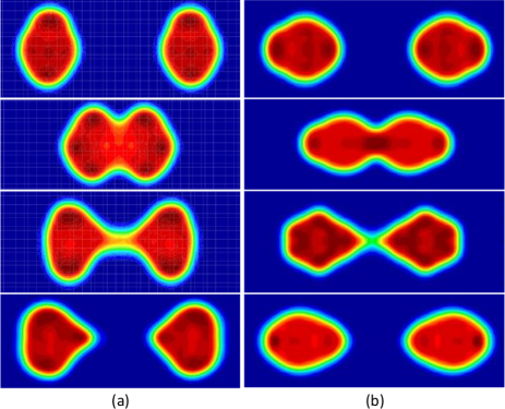
Figure 1: (Color online) Density profiles in the reaction plane in the central collisions of ²³⁸U + ²³⁸U (a) side-side collision with energy $E_{c.m.}=900$ MeV from top to bottom at times t= 0, 400, 800, and 950 fm/c, and (b) tip-tip collision with energy $E_{c.m.}=1050$ MeV from top to bottom at times t= 0, 200, 700, and 800 fm/c, respectively, obtained in TDHF calculations.

In the collision of symmetric systems, location of the window plane remains stationary, and on the average, there is no net nucleon transfer between projectile and target nuclei. According to the SMF approach, the proton and neutron numbers of the projectile-like fragment follows a stochastic evolution according to the Langevin equations,

$$\frac{d}{dt}\left(\begin{array}[]{c}{Z_{1}^{\lambda}(t)}\\ {N_{1}^{\lambda}(t)}\end{array}\right) =\int d^{3}rg(x)\left(\begin{array}[]{c}{J_{p}^{\lambda}(\vec{r},t)}\\ {J_{n}^{\lambda}(\vec{r},t)}\end{array}\right)$$ (10)

$$=\left(\begin{array}[]{c}{v_{p}^{\lambda}(t)}\\ {v_{n}^{\lambda}(t)}\end{array}\right).$$ (13)

In this expression, in place of the delta function $\delta(x)$ we introduce a Gaussian smoothing function $g(x)$ for convenience,

$$g(x)=\frac{1}{\sqrt{2\pi\kappa^{2}}}\exp\left(-\frac{x^{2}}{2\kappa^{2}}\right),$$ (14)

which approaches the delta function $\delta(x)$ in the limit $\kappa\to 0$. For the smoothing parameter, we take the value $\kappa=1$ fm. This value is in the order of lattice spacing of the numerical calculations performed in this work. The right hand side of Eq. (10) denotes the proton $v_{p}^{\lambda}(t)$ and neutron $v_{n}^{\lambda}(t)$ drift coefficients in the event $\lambda$, which are determined by the proton and the neutron current densities, $J_{p}^{\lambda}(\vec{r},t)$ and $J_{n}^{\lambda}(\vec{r},t)$, through the window in that event. In the SMF approach, the fluctuating proton and neutron currents densities in the collision direction are determined to be,

$$J_{\alpha}^{\lambda}(\vec{r},t)=\frac{\hbar}{m}\sum_{ij\in\alpha}Im\left(\Phi_{j}^{*}(\vec{r},t;\lambda)\nabla_{x}\Phi_{i}(\vec{r},t;\lambda)\right)\rho_{ji}^{\lambda}.$$ (15)

Here, and in the rest of the paper, we use the label $\alpha=p,n$ for the proton and neutron states. In the description of the SMF approach, the elements of density matrices $\rho_{ji}^{\lambda}$ are taken as uncorrelated Gaussian numbers. The mean values of the elements of density matrices are given by $\overline{\rho}_{ji}^{\lambda}=\delta_{ji}n_{j}$ and the second moments of fluctuating parts are determined by

$$\overline{\delta\rho_{ji}^{\lambda}\delta\rho_{i^{\prime}j^{\prime}}^{\lambda}}=\frac{1}{2}\delta_{ii^{\prime}}\delta_{jj^{\prime}}\left[n_{i}(1-n_{j})+n_{j}(1-n_{i})\right],$$ (16)

where $n_{j}$ are the average occupation numbers of the single-particle states.

For small amplitude fluctuations, by taking the ensemble averaging, we obtain the usual mean-field result given by the TDHF equations,

$$\frac{d}{dt}\left(\begin{array}[]{c}{Z_{1}(t)}\\ {N_{1}(t)}\end{array}\right) =\int d^{3}rg(x)\left(\begin{array}[]{c}{J_{p}(\vec{r},t)}\\ {J_{n}(\vec{r},t)}\end{array}\right)$$ (21)

$$=\left(\begin{array}[]{c}{v_{p}(t)}\\ {v_{n}(t)}\end{array}\right).$$ (24)

Here, $Z_{1}=\overline{Z}_{1}^{\lambda}$, $N_{1}=\overline{N}_{1}^{\lambda}$, $J_{\alpha}(\vec{r})=\overline{J}_{\alpha}^{\lambda}(\vec{r})$ and $v_{\alpha}=\overline{v}_{\alpha}^{\lambda}$ indicate the mean values of the proton and neutron numbers of projectile-like fragments, proton and neutron current densities, and proton and neutron drift coefficients, which are average values taken over the ensemble single-particle densities. Mean values of the current densities of protons and neutrons along the collision direction are given by,

$$J_{\alpha}(\vec{r},t)=\frac{\hbar}{m}\sum_{h\in\alpha}\text{Im}\left(\Phi_{h}^{*}(\vec{r},t)\nabla_{x}\Phi_{h}(\vec{r},t)\right),$$ (25)

where the summation $h$ runs over the occupied states originating both from the projectile and the target nuclei. Drift coefficients $v_{p}^{\lambda}(t)$ and $v_{n}^{\lambda}(t)$ fluctuate from event to event due to stochastic elements of the initial density matrix $\rho_{ji}^{\lambda}$ and also due to the different sets of the wave functions in different events. As a result, there are two sources for fluctuations of the nucleon current: (i) fluctuations those arise from the state dependence of the drift coefficients, which may be approximately represented in terms of fluctuations of proton and neutron partition of the di-nuclear system, and (ii) the explicit fluctuations $\delta v_{p}^{\lambda}(t)$ and $\delta v_{n}^{\lambda}(t)$ which arise from the stochastic part of proton and neutron currents. For small amplitude fluctuations, we can linearize the Langevin Eq. (10) around the mean evolution to obtain,

$$\frac{d}{dt}\left(\begin{array}[]{c}{\delta Z_{1}^{\lambda}(t)}\\ {\delta N_{1}^{\lambda}(t)}\end{array}\right) =\left(\begin{array}[]{c}{\frac{\partial v_{p}}{\partial Z_{1}}\left(Z_{1}^{\lambda}-Z_{1}\right)+\frac{\partial v_{p}}{\partial N_{1}}\left(N_{1}^{\lambda}-N_{1}\right)}\\ {\frac{\partial v_{n}}{\partial Z_{1}}\left(Z^{\lambda}-Z_{1}\right)+\frac{\partial v_{n}}{\partial N_{1}}\left(N_{1}^{\lambda}-N_{1}\right)}\end{array}\right)$$ (30)

$$\quad+\left(\begin{array}[]{c}{\delta v_{p}^{\lambda}(t)}\\ {\delta v_{n}^{\lambda}(t)}\end{array}\right).$$ (33)

The variances and the co-variance of neutron and proton distribution of projectile fragments are defined as $\sigma_{NN}^{2}(t)=\overline{\left(N_{1}^{\lambda}-N_{1}\right)^{2}}$, $\sigma_{ZZ}^{2}(t)=\overline{\left(Z_{1}^{\lambda}-Z_{1}\right)^{2}}$, and $\sigma_{NZ}^{2}(t)=\overline{\left(N_{1}^{\lambda}-N_{1}\right)\left(Z_{1}^{\lambda}-Z_{1}\right)}$. Multiplying both side of Eq. (30) by $N_{1}^{\lambda}-N_{1}$ and $Z_{1}^{\lambda}-Z_{1}$, and taking the ensemble average, it is possible to obtain set of coupled differential equations for the co-variances Schröder et al. (1981); Merchant and Nörenberg (1981). These differential equations are given by,

$$\frac{\partial}{\partial t}\sigma_{NN}^{2} =2\frac{\partial v_{n}}{\partial N_{1}}\sigma_{NN}^{2}+2\frac{\partial v_{n}}{\partial Z_{1}}\sigma_{NZ}^{2}+2D_{NN},$$ (34)

$$\frac{\partial}{\partial t}\sigma_{ZZ}^{2} =2\frac{\partial v_{p}}{\partial Z_{1}}\sigma_{ZZ}^{2}+2\frac{\partial v_{p}}{\partial N_{1}}\sigma_{NZ}^{2}+2D_{ZZ},$$ (35)

$$\frac{\partial}{\partial t}\sigma_{NZ}^{2} =\frac{\partial v_{p}}{\partial N_{1}}\sigma_{NN}^{2}+\frac{\partial v_{n}}{\partial Z_{1}}\sigma_{ZZ}^{2}$$

$$\quad+\sigma_{NZ}^{2}\left(\frac{\partial v_{p}}{\partial Z_{1}}+\frac{\partial v_{n}}{\partial N_{1}}\right).$$ (36)

Here, $D_{NN}$ and $D_{ZZ}$ indicate the diffusion coefficients of proton and neutron exchanges. In order to determine the co-variances in addition to the diffusion coefficients, we need to know derivatives of drift coefficients with respect to the proton and neutron numbers. These derivatives are evaluated at the mean values of the neutron and proton numbers. In symmetric collisions, mean values of the drift coefficients are zero, but in general, their slopes at the zero mean values do not vanish.

It is well know that the Langevin description is equivalent to the Fokker-Planck description of the probability distribution function $P(N,Z,t)$ primary fragments as a function of the neutron and proton numbers Hannes Risken and Till Frank (1996). When fluctuating drift coefficients are linear functions of the fluctuating proton and neutron numbers, the probability distribution of the project-like or the target-like fragments are specified by a correlated Gaussian function,

$$P(N,Z,t)=\frac{1}{2\pi\sigma_{NN}\sigma_{ZZ}\sqrt{1-\rho^{2}}}\exp\left(-C\right).$$ (37)

Here, the exponent $C$ is given by

$$C=\frac{1}{2\left(1-\rho^{2}\right)} \left[\left(\frac{Z-\overline{Z}}{\sigma_{ZZ}}\right)^{2}+\left(\frac{N-\overline{N}}{\sigma_{NN}}\right)^{2}\right.$$

$$\left.\quad-2\rho\left(\frac{Z-\overline{Z}}{\sigma_{ZZ}}\right)\left(\frac{N-\overline{N}}{\sigma_{NN}}\right)\right],$$ (38)

where $\rho=\sigma_{NZ}^{2}/\sigma_{ZZ}\sigma_{NN}$ is the correlation coefficient. The mean values $\overline{N}$, $\overline{Z}$ are the mean neutron and proton numbers of the target-like or project-like fragments.

III Transport coefficients for nucleon exchange

III.1 Quantal diffusion coefficients

The quantal expressions of the proton and neutron diffusion coefficients are determined by the correlation function of the stochastic part of the drift coefficients according to Gardiner (1991); Weiss (1999),

$$D_{\alpha\alpha}(t)=\int_{0}^{t}dt^{\prime}\overline{\delta v_{\alpha}^{\lambda}(t)\delta v_{\alpha}^{\lambda}(t^{\prime})}.$$ (39)

From Eq. (15), the stochastic parts of the drift coefficients are given by,

$$\delta v_{\alpha}^{\lambda}(t)=\frac{\hbar}{m}\sum_{ij\in\alpha}\int d^{3}rg(x)\text{Im}\left(\Phi_{j}^{*}(\vec{r},t)\nabla_{x}\Phi_{i}(\vec{r},t)\right)\delta\rho_{ji}^{\lambda}.$$ (40)

In determining the stochastic part of the drift coefficients, we impose a physical constraint on the summations of single-particle sates. The transitions among single particle states originating from projectile or target nuclei do not contribute to nucleon exchange mechanism. Therefore, in this expression, we restrict the summations as follows: when the summation $i\in T$ runs over the states originating from target nucleus, the summation $j\in P$ runs over the states originating from the projectile, and vice versa.

Using the basic postulate of the SMF approach given by Eq. (16), it is possible to calculate the correlation functions of the stochastic part of the drift coefficients, and hence we can determine the quantal expression for the diffusion coefficients. The correlation function involves a complete set of time-dependent particle and hole states. The standard solutions of TDHF give the time-dependent wave functions of the occupied hole states. The solution of complete set of time-dependent particle states requires a very large amount of effort. However, it is possible to eliminate the complete set of particle states by employing closure relation with the help of a reasonable approximation. We recognize that the time-dependent single-particle wave functions obtained from the TDHF exhibit nearly a diabatic behavior Nörenberg (1981). In other words, during short time intervals the nodal structure of time-dependent wave functions do not change appreciably. Most dramatic diabatic behavior of the time-dependent wave functions is apparent in the fission dynamics. The Hartree-Fock solutions force the system to follow the diabatic path, which prevents the system to break up into fragments. As a result of these observations, we introduce, during short time $\tau=t-t^{\prime}$ evolutions in the order of the correlation time, a diabatic approximation into the time-dependent wave functions by shifting the time backward (or forward) according to

$$\Phi_{a}(\vec{r},t^{\prime})\approx\Phi_{a}(\vec{r}-\vec{u}\tau,t),$$ (41)

where $\vec{u}$ denotes a suitable flow velocity of nucleons. Now, we can employ the closure relation,

$$\sum_{a}\Phi_{a}^{*}(\vec{r}_{1},t)\Phi_{a}(\vec{r}_{2},t^{\prime}) \approx\sum_{a}\Phi_{a}^{*}(\vec{r}_{1},t)\Phi_{a}(\vec{r}_{2}-\vec{u}\tau,t)$$

$$=\delta(\vec{r}_{1}-\vec{r}_{2}+\vec{u}\tau),$$ (42)

where, summation $a$ runs over the complete set of states originating from target or projectile, and the closure relation is valid for each set of the spin-isospin degrees of freedom. Carrying out an algebraic manipulation, we find that the quantal expressions of the proton and neutron diffusion coefficients are given by

$$D_{\alpha\alpha}(t) =\int_{0}^{t}d\tau G_{0}(\tau)\int d^{3}r\tilde{g}(x)$$

$$\quad\times\left[J_{\alpha}^{T}(\vec{r},t-\tau/2)+J_{\alpha}^{P}(\vec{r},t-\tau/2)\right]$$

$$\;\;-\int_{0}^{t}d\tau\text{Re}\left[\sum_{h^{\prime}\in P,h\in T}A_{h^{\prime}h}^{\alpha}(t)A_{h^{\prime}h}^{*\alpha}(t-\tau)\right.$$

$$\qquad\qquad\qquad\left.+\!\!\!\!\sum_{h^{\prime}\in T,h\in P}A_{h^{\prime}h}^{\alpha}(t)A_{h^{\prime}h}^{*\alpha}(t-\tau)\right],$$ (43)

where $\tilde{g}(x)=(1/\sqrt{\pi}\kappa)\exp[-(x/\kappa)^{2}]$. The quantity $J_{\alpha}^{T}(\vec{r},t-\tau/2)$ represents the sum of magnitude of the current densities due to hole wave functions originating from target nuclei,

$$J_{\alpha}^{T}(\vec{r},t)=\frac{\hbar}{m}\sum_{h\in T}|\text{Im}\left(\Phi_{h}^{*}(\vec{r},t)\nabla_{x}\Phi_{h}(\vec{r},t)\right)|.$$ (44)

Here, the quantity $G_{0}(\tau)=[1/(\tau_{0}\sqrt{4\pi})]\exp[-(\tau/2\tau_{0})^{2}]$ denotes the memory kernel with the memory time given by $\tau_{0}=\kappa/|u_{0}|$ with $u_{0}=\langle u_{h}\rangle$ as the average flow speed of hole states across the window. The quantity $J_{\alpha}^{P}(\vec{r},t-\tau/2)$ associated with the projectile states is given by a similar expression. The hole-hole matrix elements $A_{h^{\prime}h}^{\alpha}(t)$ calculated with the wave functions originating from projectile and target nuclei are given by,

$$A_{h^{\prime}h}^{\alpha}(t)=\frac{\hbar}{2m}\int d^{3}rg(x) \left[\Phi_{h^{\prime}}^{*\alpha}(\vec{r},t)\nabla_{x}\Phi_{h}^{\alpha}(\vec{r},t)\right.$$

$$\left.-\Phi_{h}^{\alpha}(\vec{r},t)\nabla_{x}\Phi_{h^{\prime}}^{*\alpha}(\vec{r},t)\right].$$ (45)

For a detailed derivation of quantal diffusion coefficients Eq. (III.1) and definition of flow velocities, we refer the reference Ayik et al. (2016). There is a close analogy between the quantal expression and the classical diffusion coefficient in a random walk problem Gardiner (1991); Weiss (1999); Randrup (1979). The first line in the quantal expression gives the sum of the nucleon currents from the target-like fragment to the projectile-like fragment and from the projectile-like fragment to the target-like fragment, which is integrated over the memory. This is analogous to the random walk problem, in which the diffusion coefficient is given by the sum of the rate for the forward and backward steps. The second line in the quantal diffusion expression stands for the Pauli blocking effects in nucleon transfer mechanism, which does not have a classical counterpart. It is important to note that the quantal diffusion coefficients are entirely determined in terms of the occupied single-particle wave functions obtained from the TDHF solutions. The quantal diffusion coefficients contain the effects of the shell structure, take into account full collision geometry and do not involve any free parameters. In the collisions at the energies we considered, the average value of nucleon flow speed across the window is $u_{0}\approx 0.05$c Ayik et al. (2016), which gives a memory time around $\tau_{0}=\kappa/u_{0}\approx 20$ fm/c. Since the memory time is much shorter than a typical interaction time of collisions, $\tau_{0}<<500$ fm/c, the memory effect is not very effective in nucleon exchange mechanism. Consequently, we can neglect the $\tau$ dependence in the current densities in Eq. (III.1), carry out the $\tau$ integration over the memory kernel to give $\int_{0}^{t}G_{0}(\tau)d\tau\approx 1/2$. Because of the same reason, memory effect is not very effective in the Pauli blocking terms as well, however in the calculations we keep the memory integrals in these terms.

III.2 Nucleon drift coefficients

In order to solve co-variances from Eqs. (34-II), in addition to the diffusion coefficients $D_{ZZ}$ and $D_{NN}$, we need to know the rate of change of drift coefficients in the vicinity of their mean values. According to the SMF approach, in order to calculate rates of the drift coefficients, we should calculate neighboring events in the vicinity of the mean-field event. Here, instead of such a detailed description, we employ the fluctuation-dissipation theorem, which provides a general relation between the diffusion and drift coefficients in the transport mechanism of the relevant collective variables as described in the phenomenological approaches Randrup (1979). Proton and neutron diffusions in the N-Z plane are driven in a correlated manner by the potential energy surface of the di-nuclear system. As a consequence of the symmetry energy, the diffusion in direction perpendicular to the beta stability valley takes place rather rapidly leading to a fast equilibration of the charge asymmetry, and diffusion continues rather slowly along the beta-stability valley. Borrowing an idea from references Nörenberg (1981); Merchant and Nörenberg (1982), we parameterize the $N_{1}$ and $Z_{1}$ dependence of the potential energy surface of the di-nuclear system in terms of two parabolic forms,

$$U(N_{1},Z_{1})= \frac{1}{2}a\left(z\cos\theta-n\sin\theta\right)^{2}$$

$$+\frac{1}{2}b\left(z\sin\theta+n\cos\theta\right)^{2}.$$ (46)

Here, $z=Z_{0}-Z_{1}$, $n=N_{0}-N_{1}$ and $\theta$ denotes the angle between beta stability valley and the $N$ axis in the $N-Z$ plane. The quantities $N_{0}$ and $Z_{0}$ denote the equilibrium values of the neutron and proton numbers, which are approximately determined by the average values of the neutron and proton numbers of the projectile and target ions, $N_{0}=\left(N_{P}+N_{T}\right)/2$ and $Z_{0}=\left(Z_{P}+Z_{T}\right)/2$. The first term in this expression describes a strong driving force perpendicular to the beta stability valley, while the second term describes a relative weak driving force toward symmetry along the valley. In symmetric collisions, $N_{0}$ and $Z_{0}$ are equal to the initial neutron and proton numbers of the target or projectile nuclei. Following from the fluctuation-dissipation theorem, it is possible to relate the proton and neutron drift coefficients to the diffusion coefficients and the associated driving forces, in terms of the Einstein relations as follows Nörenberg (1981); Merchant and Nörenberg (1982),

$$\nu_{n} =-\frac{D_{NN}}{T}\frac{\partial U}{\partial N_{1}}=+\frac{D_{NN}}{T}\frac{\partial U}{\partial n}$$

$$=D_{NN}\left[-\alpha\sin\theta\left(z\cos\theta-n\sin\theta\right)\right.$$

$$\qquad\qquad\left.+\beta\cos\theta\left(z\sin\theta+n\cos\theta\right)\right],$$ (47)

and

$$\nu_{z} =-\frac{D_{ZZ}}{T}\frac{\partial U}{\partial Z_{1}}=+\frac{D_{ZZ}}{T}\frac{\partial U}{\partial z}$$

$$=D_{ZZ}\left[+\alpha\cos\theta\left(z\cos\theta-n\sin\theta\right)\right.$$

$$\qquad\qquad\left.+\beta\sin\theta\left(z\sin\theta+n\cos\theta\right)\right].$$ (48)

Here, the temperature $T$ is absorbed into coefficients $\alpha$ and $\beta$, consequently temperature does not appear as a parameter in the description. In asymmetric collisions, it is possible to determine $\alpha$ and $\beta$ by matching the mean values of neutron and proton drift coefficients obtained from the TDHF solutions. In symmetric collisions, the mean value of drift coefficients are zero and the mean values of neutron and proton numbers do not change and remain equal to their initial values. Therefore it is not possible to determine the coefficients $\alpha$ and $\beta$ from the full TDHF solutions. However, we can determine these coefficients employing the one-sided neutron and proton fluxes from projectile-like fragment to the target-like fragment or vice-versa. We indicate neutron and proton numbers of one of the fragments as $\tilde{N}_{1}$ and $\tilde{Z}_{1}$. Then, the neutron and proton numbers of this fragment monotonically decreases according to,

$$\frac{d}{dt}\left(\begin{array}[]{c}{\tilde{Z}_{1}(t)}\\ {\tilde{N}_{1}(t)}\end{array}\right) =\int d^{3}rg(x)\left(\begin{array}[]{c}{\tilde{J}_{p}(\vec{r},t)}\\ {\tilde{J}_{n}(\vec{r},t)}\end{array}\right)$$ (53)

$$=\left(\begin{array}[]{c}{\tilde{v}_{p}(t)}\\ {\tilde{v}_{n}(t)}\end{array}\right).$$ (56)

Here, $\tilde{v}_{\alpha}(t)$ with $\alpha=n,p$ denotes the one-sided neutron and proton drift coefficients towards the other fragment and the one-sided current density $\tilde{J}_{\alpha}(\vec{r},t)$ is given by Eq. (25) keeping only negative terms in the summation over the hole states. The one-sided drift coefficients $\tilde{\nu}_{n}$ and $\tilde{\nu}_{p}$ are related to the driving force with the similar expressions given by Eq. (III.2) and Eq. (III.2), except that $n$ and $z$ are replaced by $\tilde{n}=N_{0}-\tilde{N}_{1}$ and $\tilde{z}=Z_{0}-\tilde{Z}_{1}$ and by including an overall sign change,

$$\tilde{\nu}_{n}=D_{NN} \left[+\alpha\sin\theta\left(\tilde{z}\cos\theta-\tilde{n}\sin\theta\right)\right.$$

$$\;\left.-\beta\cos\theta\left(\tilde{z}\sin\theta+\tilde{n}\cos\theta\right)\right],$$ (57)

and

$$\tilde{\nu}_{z}=D_{ZZ} \left[-\alpha\cos\theta\left(\tilde{z}\cos\theta-\tilde{n}\sin\theta\right)\right.$$

$$\;\left.-\beta\sin\theta\left(\tilde{z}\sin\theta+\tilde{n}\cos\theta\right)\right].$$ (58)

Fig. 2 shows the one-sided mean-drift paths of projectile-like fragments which are determined by keeping the one-sided neutron and proton fluxes from projectile-like to the target-like fragments in the side-side and tip-tip collisions of ²³⁸U + ²³⁸U.

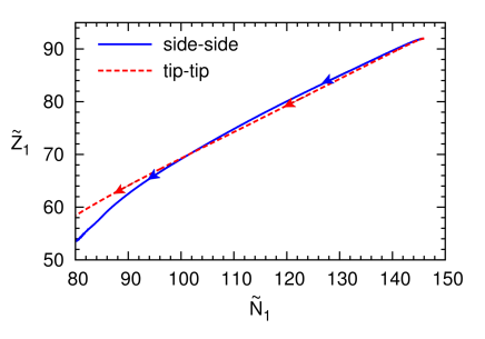
Figure 2: (Color online) Mean drift path of the projectile-like fragments in $N-Z$ plane in the central collisions of ²³⁸U + ²³⁸U at side-side collision with energy $E_{c.m.}=900$ MeV (solid line), and at tip-tip collision with energy $E_{c.m.}=1050$ MeV (dashed line), obtained with one-sided flux in TDHF calculations.

Using this information, we can extract the angle $\theta$ and the magnitude of coefficients $\alpha$ and $\beta$. We find that, the angle between the mean one-sided drift path and $N$-axis is about $\theta\approx 30^{\circ}$ in both collision geometries. As a result of the quantal effects arising mainly from the shell structure, we observe that the coefficients $\alpha$ and $\beta$ exhibit fluctuations as a function of time. In the side-side collision, during the relevant time interval from $200$ fm/c to $800$ fm/c, the average values of these coefficients are about $\alpha\approx 0.035$ and $\beta\approx 0.007$. In the tip-tip collision, during the relevant time interval from $200$ fm/c to $700$ fm/c, the average values of these coefficients are about $\alpha\approx 0.039$ and $\beta\approx 0.009$. These results are consistent with the potential energy surface of the liquid drop picture. The potential energy surface in (N-Z) plane has a steeply rising parabolic shape in the perpendicular direction to the stability valley and has a shallow behavior along the stability valley. Because of a simple analytical structure, we can easily calculate derivatives of drift coefficients which are needed in differential Eqs. (34-II) for determining the co-variances.

IV Primary fragment distributions

In determining the primary fragment distributions, the main input quantities are the neutron and proton diffusions coefficients given in Eq. (III.1). The diffusion coefficients are entirely determined by the occupied time-dependent single-particle states. The TDHF theory includes the one-body dissipation mechanism. We can use the same information provided by the TDHF to calculate the diffusion coefficients which describe the fluctuation mechanism of the collective motion. The reason behind this fact is the fundamental relation that exists between dissipation and fluctuation mechanism of the collective motion as stated in the fluctuation-dissipation theorem Gardiner (1991); Weiss (1999). Fig. 3 shows the neutron (solid lines) and proton (dashed lines) diffusion coefficients in the side-side and the tip-tip central collisions of ²³⁸U + ²³⁸U at bombarding energies $E_{c.m.}=900$ MeV and $E_{c.m.}=1050$ MeV, respectively.

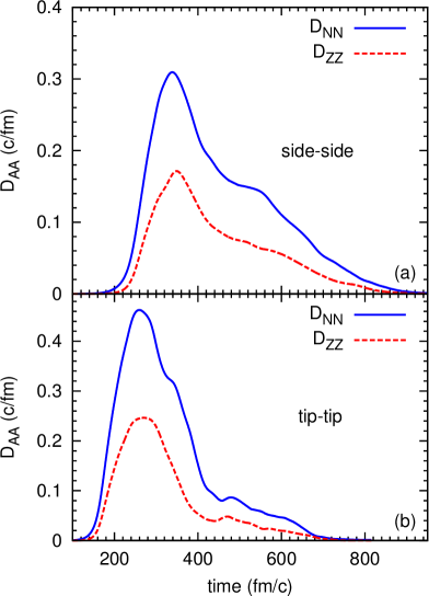
Figure 3: (Color online) Neutron and proton diffusion coefficients in the central collisions of ²³⁸U + ²³⁸U (a) side-side collision with energy $E_{c.m.}=900$ MeV, and (b) tip-tip collision with energy $E_{c.m.}=1050$ MeV, respectively.

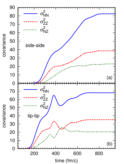
Figure 4: (Color online) Neutron, proton co-variances in the central collisions of ²³⁸U + ²³⁸U (a) side-side collision with energy $E_{c.m.}=900$ MeV, and (b) tip-tip collision with energy $E_{c.m.}=1050$ MeV, respectively.

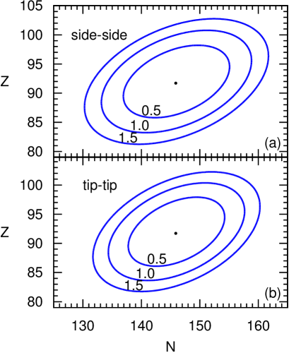
Figure 5: (Color online) Equal probability lines for primary fragment formation with $C=0.5$, $1.0$, $1.5$ in the central collisions of ²³⁸U + ²³⁸U (a) side-side collision with energy $E_{c.m.}=900$ MeV, and (b) tip-tip collision with energy $E_{c.m.}=1050$ MeV, respectively.

We determine the proton, neutron co-variance by solving the coupled differential Eqs. (34-II) with the initial conditions $\sigma_{nn}(0)=0$, $\sigma_{pp}(0)=0$ and $\sigma_{np}(0)=0$. Fig. 4 illustrates these co-variance as a function of time in the side-side and the tip-tip central collisions of ²³⁸U + ²³⁸U. Primary fragment distribution in $N-Z$ plane is determined by a correlated Gaussian given by Eq. (37). The elliptic curves in Fig. 5 show equal probability lines relative to the center point for producing fragments for three values of the exponent $C=0.5$, $1.0$, $1.5$ in the Gaussian function. For example the probability for producing fragments on the ellipse with $C=0.5$ relative to the symmetric fragmentation is $\exp(-0.5)=0.6$. Primary fragment distributions have a similar behavior in both side-side and tip-tip collisions as seen from panels (a) and (b). The variance of fragment mass distributions is determined by

$$\sigma_{AA}^{2}(t)=\sigma_{NN}^{2}(t)+\sigma_{ZZ}^{2}(t)+2\sigma_{NZ}^{2}(t).$$ (59)

As seen from Fig. 4, at the end of the final states of collisions the co-variances of the fragment mass distribution have the values $\sigma_{AA}(t)=12.9$ and $\sigma_{AA}(t)=12.0$ in side-side and tip-tip collisions, respectively. Fig. 6 illustrates the Gaussian form of the mass distributions of the primary fragments with a mean value $\overline{A}=238$ and variances $\sigma_{AA}(t)=12.9$ and $\sigma_{AA}(t)=12.0$.

In the symmetric fragmentation of the final state, we can determine the excitation energy of each final ²³⁸U nucleus by calculating the final total kinetic energy ($TKE$) from the TDHF solutions. We find $TKE=620$ MeV and $TKE=634$ MeV in the side-side and the tip-tip collisions, respectively. From the energy conservation, $E^{*}=E_{cm}-TKE$, we find that the excitation energy of each ²³⁸U nucleus is $E^{*}=140$ MeV and $E^{*}=208$ MeV, in the side-side and the tip-tip collisions. As a result of multi-nucleon transfer in the collisions, there are many binary fragments in the final state as indicated in distributions in Fig. 5.

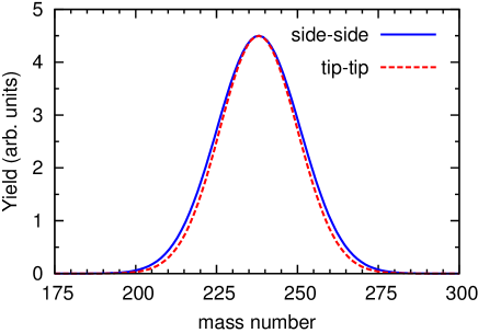
Figure 6: (Color online) Primary fragment mass distributions in the central collisions of ²³⁸U + ²³⁸U at side-side collision with energy $E_{c.m.}=900$ MeV (solid line) and at tip-tip collision with energy $E_{c.m.}=1050$ MeV (dashed line).

In the present work, we cannot calculate the excitation energies of each final fragment pair, but we can estimate them by using the Viola systematics. It is very reasonable to assume that all available initial relative kinetic energy is dissipated into the internal excitations and is shared between the fragments in proportion to the ratio of masses in possible final binary channel. According to the Viola formula, total excitation $E_{c}^{*}$ in a binary channel is determined by $E_{c}^{*}=E_{cm}+Q_{c}-(TKE)_{c}$. Here, $Q_{c}$ is the Q-value of the binary channel and $(TKE)_{c}$ indicates the total final kinetic energy of fragments. $(TKE)_{c}$ is approximately determined by Coulomb potential energy of the binary fragments at an effective relative distance determined by an adjustable parameter $r_{0}$ as,

$$(TKE)_{c}=\frac{1}{4\pi\varepsilon_{0}}\frac{Z_{1c}Z_{2c}e^{2}}{r_{0}\left(A_{1c}^{1/3}+A_{2c}^{1/3}\right)}.$$ (60)

With help of $TKE$ of the symmetric binary channel, we adjust the parameter $r_{0}=1.59$ fm and $r_{0}=1.55$ fm for the side-side and tip-tip collisions, respectively. We estimate that primary fragments inside the eliptic region with $C=1.5$ have excitation energies in the range of $(120-150)$ MeV and $(185-225)$ MeV in the side-side and tip-tip collisions, respectively. Highly exited intermediate mass fragments cool down by particle evaporations and heavy-fragments should immediately fission. However we do not perform de-excitation calculations of the primary fragments in this work.

V Conclusions

The SMF approach improves the standard mean-field description by incorporating thermal and quantal fluctuations in the collective motion. The approach requires to generate an ensemble of mean field trajectories. The initial conditions for the events in the ensemble are specified by the quantal and thermal fluctuations in the initial state in a suitable manner, and each event is evolved by its own self-consistent mean-field Hamiltonian. In reactions where the colliding system maintains a di-nuclear structure, the reaction dynamics can be described in terms of a set of relevant macroscopic variables, which can be defined with the help of the window dynamics. The SMF approach gives rise to a quantal Langevin description for the evolution of the macroscopic variables. In this work, we apply this approach and analyze multi-nucleon transfer mechanism in the central collisions of ²³⁸U + ²³⁸U in side-side geometry with energy $E_{c.m.}=900$ MeV and in tip-tip geometry with energy $E_{c.m.}=1050$ MeV. Fluctuation mechanism of neutron and proton exchanges is described by the quantal diffusion coefficients. Quantal diffusion coefficients are entirely determined by the single-particle states of the TDHF equations. These coefficients include the full geometry of the collision process and the effect of the shell structure. They do not involve any adjustable parameters and do not require any additional information. Deep underlying reason behind this is the fact that the dissipation and fluctuation aspects of the dynamics are connected according to the fluctuation-dissipation theorem of non-equilibrium statistical mechanics. We estimate the excitation energies of the primary fragments with the help of Viola formula which provides an approximate description of the total final kinetic energy of the binary fragments. The highly excited fragments are cooled down by particle emission and in particular highly excited heavy fragments are expected to decay rapidly by fission. We plan to carry out de-excitation calculations and determine the secondary fragment distributions in a subsequent work.