The localization transition in SU(3) gauge theory

Abstract

We study the Anderson-like localization transition in the spectrum of the Dirac operator of quenched QCD. Above the deconfining transition we determine the temperature dependence of the mobility edge separating localized and delocalized eigenmodes in the spectrum. We show that the temperature where the mobility edge vanishes and localized modes disappear from the spectrum, coincides with the critical temperature of the deconfining transition. We also identify topological charge related close to zero modes in the Dirac spectrum and show that they account for only a small fraction of localized modes, a fraction that is rapidly falling as the temperature increases.

I Introduction

Quantum Chromodynamics (QCD), the theory of strong interactions, has a rich structure even at zero chemical potential. At low temperature quarks are confined in hadrons, while at high enough temperature they are liberated and form a quark-gluon plasma. The hadronic and plasma phases are not separated by a genuine phase transition, only a rapid cross-over occurs in between, where quarks become deconfined Borsanyi:2010bp . This deconfining transition is also accompanied by the restoration of the approximate chiral symmetry that is spontaneously broken at low temperature.

It is well-known that at low temperature eigenstates of the quark Dirac operator are delocalized and the corresponding eigenvalues are described by Wigner-Dyson statistics known from random matrix theory (see eg. Verbaarschot:2000dy for a review). Already a long time ago speculations appeared that the finite temperature chiral transition might be accompanied or even driven by an Anderson-type localization transition in the lowest part of the Dirac spectrum Halasz:1995vd . If this happens, the lowest eigenmodes of the Dirac operator become localized and the corresponding part of the spectrum is described by Poisson statistics. It was only a decade later that the first evidence for such a transition was obtained both in an instanton liquid model GarciaGarcia:2005vj and in lattice simulations GarciaGarcia:2006gr . In both cases it was found that when the system crosses into the high temperature phase, the spectral statistics starts to move from Wigner-Dyson towards Poisson. However, in the lattice simulation the used volumes were not large enough to allow a precise quantitative assessment of the localization transition.

Later on more quantitative lattice studies of the transition appeared both in QCD and other similar models, and features of an Anderson transition were confirmed in more detail (see Giordano:2014qna for a review). It was found that at temperatures well above the transition the lowest part of the Dirac spectrum consists of spatially localized eigenmodes, while eigenmodes higher up in the spectrum are delocalized. Exactly as in the case of Anderson-type models, the localized and delocalized modes are separated by a critical point in the spectrum, the so called mobility edge Kovacs:2012zq . The transition at the mobility edge turned out to be a genuine second order transition characterized by a correlation length critical exponent compatible with that of the three dimensional Anderson model of the same symmetry class Giordano:2013taa .

When the temperature is lowered towards the chiral transition, the mobility edge within the spectrum moves down towards the origin. At the temperature where the mobility edge vanishes, all the localized modes disappear from the spectrum and even the lowest part of the spectrum becomes delocalized. We note that this disappearance of localized modes at some temperature is expected, as we know that at zero temperature the whole spectrum consists of delocalized modes. However, what is remarkable is that this localization transition occurs in the crossover temperature region. We emphasize that on the one hand, the vanishing of the mobility edge happens at a precisely defined temperature. On the other hand, the chiral transition is only a cross-over and no precise critical temperature can be associated with it. Therefore in QCD the question of whether the chiral and the localization transition happen at exactly the same temperature, is not meaningful.

There are, however, models similar to QCD where a genuine finite temperature chiral or deconfining phase transition does take place. An example is QCD with staggered quarks on coarse lattices $(N_{t}=4)$. This system possesses a genuine phase transition in the thermodynamic limit, as the spatial box size goes to infinity while the temporal size is kept fixed at $N_{t}=4$ Nt4 . Here it was shown that the disappearance of localized modes at the low-end of the Dirac spectrum precisely coincides with the chiral phase transition Giordano:2016nuu . However, the chiral phase transition of $N_{t}=4$ staggered quarks does not survive in the continuum limit.

QCD in the limit of large quark masses, i.e. the quenched theory is another example of a QCD-like system with a genuine deconfining phase transition. In the present paper we focus on this system, SU(3) Yang-Mills theory and study how the Anderson-type localization transition is related to the finite temperature deconfining phase transition. An advantage of this model compared to the one mentioned above is that in this case the phase transition survives the continuum limit. The main result of the present paper is that the lowest eigenmodes of the Dirac operator are found to become localized exactly at the critical temperature of the deconfining transition.

We show this by simulating SU(3) lattice gauge theory at different temperatures above the deconfining phase transition. We compute the low part of the spectrum of the Dirac operator on these gauge configurations. For the gauge ensembles at each temperature we find the mobility edge by analyzing the unfolded level spacing distribution. In this way we compute the mobility edge as a function of the temperature (or rather, the inverse gauge coupling $\beta$) and by extrapolation we find the temperature where the mobility edge vanishes. This is the critical temperature of the localization transition where localized quark modes completely disappear from the spectrum. Below this temperature even the lowest Dirac eigenmodes are delocalized. We find that the gauge coupling where this happens is compatible with the critical coupling of the deconfining transition. This demonstrates that indeed the localization and the deconfining transition are strongly related.

Another question we would like to touch upon here concerns the nature of the localized eigenmodes of the Dirac operator and the possible role instantons might play in the localization transition. A plausible understanding of the QCD vacuum holds that low eigenmodes of the Dirac operator are essentially linear combinations of approximate instanton and antiinstanton zero modes Schafer:1996wv . In this framework the localization transition might be understood as follows. In the Euclidean formulation of QCD the temperature is set by the temporal size of the box as

$$T=\frac{1}{aN_{t}},$$ (1)

where $N_{t}$ is the temporal box size in lattice units and $a$ is the physical lattice spacing. As the temperature is increased above the cross-over temperature, the temporal box size become too small for instantons of typical size and they are effectively squeezed out of the system. As a result, above the cross-over the instanton density drastically decreases and the corresponding approximate zero modes, i.e. the low-end of the Dirac spectrum is depleted. Due to the lower instanton density and smaller instanton size the quarks cease to be able to hop from instanton to instanton and get localized. It was verified in a numerical simulation that an instanton gas with realistic QCD parameters is indeed capable of producing such a transition GarciaGarcia:2005vj .

If this picture is valid, the localized Dirac eigenmodes are essentially approximate instanton zero modes. To resolve instantons, a fine enough grid is needed, therefore the quenched theory where the phase transition survives in the continuum limit, is well suited for studying the role of instanton zero modes. Our results indicate that already at $N_{t}=6$, above the critical temperature quark eigenmodes connected to instantons can be separated from the rest of the spectrum, as they show up as a bump in the spectral density around zero. We demonstrate that these zero mode related quark eigenmodes account only for a fraction of the localized modes and that fraction becomes ever smaller as the temperature increases. This indicates that even in the quenched theory where instantons are expected to be more abundant than in full QCD, zero modes do not account for the localized quark modes.

The plan of the paper is as follows. In Section II we briefly summarize the details of our lattice simulations. In Section III we discuss the mobility edge and how it can be computed using the unfolded level spacing distribution. In Section IV we present our main result, the dependence of the mobility edge on the gauge coupling. By extrapolation we determine the critical coupling where the mobility edge vanishes. We perform the analysis at three different lattice spacings, corresponding to $N_{t}=4,6$ and $8$, and find that in all cases the critical coupling for localization is compatible with the point where the deconfining transition occurs. In Section V we show that instanton-related low modes can be separated in the spectrum but most likely they cannot explain the localized quark modes found at high temperatures. Finally, in Section VI we discuss our conclusions and some further questions not addressed in the present paper.

II Details of the simulation

We simulate SU(3) lattice gauge theory with the Wilson plaquette action on lattices of temporal extent $N_{t}=4,6$ and $8$. In all three cases we use several values of the gauge coupling just above the finite temperature deconfining transition. To assess finite volume effects, at each gauge coupling we consider at least two different spatial volumes. The deconfining transition is of first order and the correlation length does not diverge, but our experience shows that it increases substantially towards the transition. Therefore, closer to the transition we need to use larger volumes. We choose the volumes by the requirement that the physical quantity we are interested in, the mobility edge, be volume independent within the statistical errors. We summarize the parameters of our simulations in Table 1.

$N_{t}$	$\beta$	$N_{s}$	Nconf	Nevs
4	5.693	32	1061	600
		40	1192	1100
		48	2381	1500
	5.694	32	1715	600
		40	1005	1100
		48	2014	1600
	5.695	32	2184	650
		40	2012	1100
		48	2028	1300
	5.696	32	1073	900
		40	1628	1000
	5.6975	32	2291	600
		40	1524	1100
		48	2000	1500
	5.6985	40	1973	1000
	5.7	24	4139	600
		32	4040	800
		40	1022	1000
	5.71	24	2509	300
		32	2507	450
		40	1073	1100
	5.74	24	2024	300
		32	2501	450
		40	2390	1100
6	5.897	32	532	900
		40	1249	1000
		48	682	1350
	5.9	32	998	900
		40	925	1000
		48	813	1350
	5.91	32	1068	900
		40	834	1000
		48	1088	1350
	5.92	32	1822	600
		40	960	1000
	5.93	32	806	900
		40	1050	1000
	5.94	40	1092	1000
	5.95	32	562	600
		40	1276	1000
	5.96	32	832	1000
		40	1032	1000
	6.0	32	1392	900
		40	1958	1000
8	6.1	48	439	500
		56	681	600
		64	486	400
	6.15	48	781	500
		56	698	600
		64	385	400
	6.18	48	636	500
		56	964	600
		64	384	400
	6.2	48	675	500
		56	778	600
		64	418	400
	6.25	48	758	500
		56	652	600
		64	320	400
	6.3	48	578	500
		56	616	600
		64	452	400

Table 1: The parameters of the simulations; the temporal size of the lattice, the Wilson plaquette gauge coupling, the spatial size of the box, the number of configurations and the number of Dirac eigenvalues computed on each gauge configuration.

We calculate the lowest eigenvalues of the Dirac operator on these gauge configurations. The lattice Dirac operator we consider is the staggered operator on two times stout smeared gauge links with smearing parameter $\rho=0.15$ Aoki:2005vt . The spectrum of the staggered operator (at zero quark mass that we consider here) is purely imaginary and symmetric around zero. Therefore, we will only compute the positive eigenvalues. The number of eigenvalues we calculate on each configuration is set by the requirement to capture all the localized modes and also the transition region from localized to delocalized modes. This is needed for a precise determination of the mobility edge on each ensemble.

III Calculation of the mobility edge

At high temperature the lowest part of the Dirac spectrum consists of localized eigenmodes, while higher up in the spectrum the eigenmodes are delocalized. The boundary between localized and delocalized modes is the mobility edge, $\lambda_{c}$. In QCD if the temperature is lowered towards the transition, the mobility edge shifts down towards zero and at a certain temperature in the cross-over region it reaches zero. At this point localized modes completely disappear from the spectrum and even the lowest eigenmodes becomes delocalized. We expect similar behavior in the quenched theory. Our main goal is to determine the temperature at which the mobility edge hits zero and all Dirac modes become delocalized.

To this end we calculate the mobility edge as a function of the temperature and by extrapolation find the temperature at which $\lambda_{c}(T)=0$. Since strictly speaking in the quenched theory it is not possible to set a physical scale, we actually compute the mobility edge as a function of the Wilson gauge coupling $\beta$ and find the gauge coupling where $\lambda_{c}(\beta)$ becomes zero. This can be compared to the known critical gauge coupling $\beta_{c}\textsuperscript{deconf}$, where the deconfining transition takes place.

On an ensemble of gauge configurations obtained at a given gauge coupling $\beta$ we use the following procedure to determine the mobility edge. The simplest way to tell whether the eigenmodes are localized or not is to consider the unfolded level spacing distribution. After unfolding, which is a rescaling of the level spacings by their local average (local in the spectrum), the resulting distribution is known to be universal. In the case of localized modes it is the exponential distribution $p(s)=\exp(-s)$ following from an uncorrelated spectrum. In contrast, the level spacing distribution of delocalized modes can be accurately described by the unitary Wigner surmise

$$P_{\mbox{\scriptsize u}}(s)=\dfrac{32}{\pi^{2}}s^{2}\cdot\exp\left(-\dfrac{4}{\pi}s^{2}\right)$$ (2)

corresponding to the symmetry class of the Dirac operator at hand Verbaarschot:2000dy (see Fig. 1).

Figure 1: The exponential distribution (dashed line) of level spacings for localized eigenmodes and the unitary Wigner surmise of Eq. (2) (solid line) describing the level spacing distribution of delocalized modes.

Since we would like to detect a transition from localized to delocalized modes within the spectrum, the spectral statistics have to be computed locally. We do this by subdividing the spectrum into small intervals of width $\Delta\lambda$ and considering the level spacing distribution separately in each subinterval as a function of its location in the spectrum. As we move up in the spectrum and the eigenmodes change from localized to delocalized, the exponential distribution of level spacings continuously deforms into the Wigner surmise. To follow this more quantitatively it is convenient to consider a single quantity characterizing the continuously deforming distribution. We choose

$$I_{s_{0}}=\int_{0}^{s_{0}}p(s)\,d\!s,$$ (3)

where the upper limit of the integration was taken to be $s_{0}=0.508$, the point where the exponential and the Wigner surmise probability densities first intersect. This choice was made to maximize the difference in this parameter between the two limiting distributions. In Fig. 2 we show a typical plot of how this quantity changes across the spectrum interpolating from the value corresponding to the exponential distribution to the Wigner surmise. In the Figure we show $I_{s_{0}}$ for different volumes. It is apparent that as the volume increases the cross-over from localized to delocalized modes becomes sharper. In fact, in QCD a finite-size scaling study revealed that in the infinite volume limit the transition is of second order Giordano:2013taa .

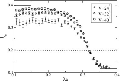
Figure 2: The quantity $I_{s_{0}}(\lambda)$ as a function of the location in the spectrum. $I_{s_{0}}$ shows how the level spacing distribution changes from exponential to Wigner surmise as the eigenmodes change from localized to delocalized across the spectrum. The solid line segments in the upper left and lower right corners indicate the limiting values for the exponential and the Wigner-Dyson distributions. The dotted line corresponds to the critical value of $I_{s_{0}}$. Data is shown for $N_{t}=4,\beta=5.74$ in three different lattice volumes with the larger symbols corresponding to larger volumes.

Our main concern here is the determination of the critical point $\lambda_{c}$ in the spectrum where the transition from localized to delocalized modes happens in the infinite volume limit. We identify the critical point with the location in the spectrum where $I_{s_{0}}$ reaches the value $I_{s_{0}cr}=0.196$ corresponding to the critical statistics between the Poisson and Wigner-Dyson statistics Shapiro:1993 . Since in the thermodynamic limit the transition becomes infinitely sharp, instead of $I_{s_{0}cr}$, any other value between the one corresponding to the Poisson and the Wigner-Dyson statistics could have been chosen. However, our choice turns out to have small finite size corrections. Another advantage of our choice is that around the point $I_{s_{0}cr}$ the curve $I_{s_{0}}(\lambda)$ has an inflection point and it is well approximated by a straight line. Therefore in the vicinity of this point a linear fit to the data can be used to obtain a precise determination of the solution to the equation $I_{s_{0}}(\lambda)=I_{s_{0}cr}$.

We did this for several choices of $\Delta\lambda$, the width of the spectral windows where $I_{s_{0}}$ was computed. Since the spectral statistics changes along the spectrum, $\Delta\lambda$ had to be small enough to have this change negligible within this spectral window. Besides this, there is a trade-off in the choice of $\Delta\lambda$; narrower spectral windows yield more data points, however each data point has a larger statistical error, due to the smaller number of eigenvalues falling in each spectral window and as a result, a smaller statistics. We chose different values of $\Delta\lambda$ and found that within reasonable bounds $0.0005\leq a\,\Delta\lambda\leq 0.005$ the resulting variation in $\lambda_{c}$ was well below the statistical uncertainty. The latter was estimated using the jackknife method.

This procedure yielded $\lambda_{c}$ for each lattice ensemble. To keep finite volume corrections under control, we increased the spatial linear size of the lattice in steps of $8$ until the resulting $\lambda_{c}$ did not change any more to within the statistical errors. Not surprisingly, closer to the deconfining temperature larger volumes were needed for that.

IV The critical temperature of localization

To determine the dependence of the mobility edge, $\lambda_{c}$, on the inverse gauge coupling $\beta$, we repeated the above procedure for different values of $\beta$ above the deconfining temperature. As an illustration, in Fig. 3 we show $\lambda_{c}$ versus $\beta$ for the lattices of temporal size $N_{t}=4$. The analogous graphs for other values of $N_{t}$ are qualitatively similar. In order to determine $\beta_{c}\textsuperscript{loc}$, the critical coupling for the localization transition, we fitted the parameters $b,c$ and $\beta_{c}$ of the function

$$a\,\lambda_{c}(\beta)=c\,(\beta-\beta_{c}\textsuperscript{loc})^{b}$$ (4)

to the data points. The fit range was chosen by two criteria. The lower end was restricted because close to the deconfining transition larger volumes were needed and here we included only those points where simulations could be done on large enough volumes to ensure no finite volume corrections to $\lambda_{c}$. The upper end of the fit range was limited by the fact that the chosen functional form of $\lambda_{c}(\beta)$ had a finite range of validity. At the upper end we included as many data points as was possible to keep the quality of the fit (measured by the $\chi^{2}$) acceptable. In the Figure we show only the points that were used for the fit. Since all the data points used originated from independent simulations, performed at different values of the gauge coupling, they are also statistically independent and the uncertainty of the fit parameters could be easily estimated.

Figure 3: The mobility edge $\lambda_{c}a$ (in lattice units) as a function of the inverse gauge coupling for temporal lattice size $N_{t}=4$. The solid line is a fit to the data using the function in Eq. (4).

In Table 2 we give the main result of the paper, the critical gauge coupling, where localized eigenmodes disappear from the spectrum. In comparison we also quote the critical coupling for the deconfining transition which is known from the literature Francis:2015lha . Clearly the critical couplings for the deconfining and the localization transition coincide to within the numerical uncertainties. Moreover, this happens for $N_{t}=4,6$ and $8$, i.e. at three different lattice spacings. We would like to point out that according to present-day standards of QCD thermodynamics simulations, even $N_{t}=8$ lattices around $T_{c}$ are not considered to be very fine lattices. However, since in the quenched theory the transition happens at a relatively higher temperature than in full QCD, these lattices are not very coarse. Indeed, at the critical point for $N_{t}=8$ the lattice spacing set by the Sommer scale Sommer:1993ce , $r_{0}$ is $a=0.085$ fm. Our $N_{t}=8$ simulations are performed on even finer lattices with $0.07$ fm$<a<0.08$ fm. It is thus very likely that the same behavior persists in the continuum limit. This provides strong evidence that the deconfining and the localization transition are linked.

$N_{t}$	$\beta_{c}$deconf	$\beta_{c}$loc	b	c	fit range
4	5.69254(24)	5.69245(17)	0.1861(6)	0.563(2)	5.695-5.71
6	5.8941(5)	5.8935(16)	0.1580(8)	0.320(1)	5.91-5.96
8	6.0624(10)	6.057(4)	0.164(4)	0.233(2)	6.08-6.18

Table 2: The critical gauge couplings where the deconfining and the localization transition occur for temporal lattice sizes of $N_{t}=4,6$ and $8$. We also list the fit parameters $b$ and $c$ appearing in Eq. (4), as well as the best fit range in $\beta$, selected by the criteria described in the text.

V Localized modes and instantons

In the present Section we would like to study the possible relationship between instanton-antiinstanton zero modes and localized modes. The simplest question that arises in this connection is how the number of localized modes compares with that of the topology related eigenmodes. Since we computed the mobility edge for each ensemble, the average number of localized modes per configuration, i.e. the number of eigenvalues below the mobility edge can be easily counted.

A more difficult question is how to separate the topology related modes from the rest of the spectrum. In fact, above the deconfining transition where the instantons form a dilute gas, this is possible by looking at the spectral density of a Dirac operator with sufficiently good chiral properties. Indeed, it was found that the eigenvalues corresponding to approximate instanton and antiinstanton zero modes show up in the spectrum of the overlap Dirac operator as a bump in the spectral density close to zero Edwards:1999zm . We emphasize that these eigenmodes are not the zero modes corresponding to the net topological charge, but small complex eigenvalues of the overlap Dirac operator produced by a dilute gas of instantons and antiinstantons. More recently a very detailed study of this part of the spectrum appeared and it was found that this feature in the spectrum persists even if dynamical fermions are present Alexandru:2015fxa .

In Fig. 4 we show the spectral density of the Dirac operator used in the present paper on $N_{t}=6,8$ and 10 lattices just above the deconfining transition at $T=1.05T_{c}$. We set the scale using the Sommer parameter, $r_{0}=0.49$ fm. Already for $N_{t}=6$ the instanton related modes appear to be separated from the bulk of the spectrum and this separation becomes even more pronounced on the finer lattices. We note here that in Ref. Edwards:1999zm this spectral structure around zero was seen only with the overlap operator but not in the spectrum of the staggered operator. However, the lattices we use here are finer, and in contrast to Ref. Edwards:1999zm , we use an improved staggered operator with two times stout smeared gauge links. Apparently the finer lattices and the improved staggered operator make it possible to resolve zero modes and separate them from the bulk of the spectrum . In what follows we consider those modes to be instanton related that are below the minimum between the bump at the origin and the bulk of the spectrum.

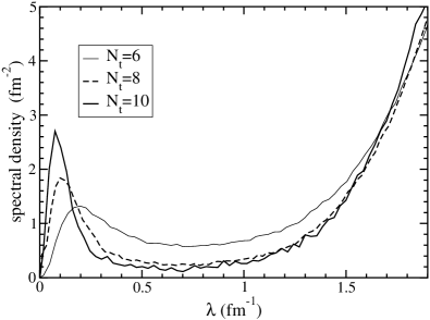
Figure 4: The spectral density of the Dirac operator at a temperature slightly above the deconfining phase transition $(T=1.05T_{c})$. The data sets represent data for different lattice spacings corresponding to temporal lattice sizes of $N_{t}=6,8$ and $10$. The density is understood to be normalized with the three-dimensional (spatial) volume.

Now we can compare the number of topology related small modes and the total number of localized eigenmodes. In Fig. 5, as a function of the temperature in units of $T_{c}$, we plot the fraction of localized modes accounted for by instantons and antiinstantons on the $N_{t}=6$ and $N_{t}=8$ lattices. In the same figure we also included a data point on a finer, $N_{t}=10$ lattice. By extrapolating the data down to the critical temperature, we estimate that just above the deconfining transition about 60% of the localized modes can be identified as topology related near zero modes. As the temperature increases, this fraction falls rapidly. Clearly, above the deconfining transition most of the localized low modes cannot be identified with instanton related close to zero modes. This is especially true farther above the critical temperature. Within our numerical accuracy the data appears to be scaling which indicates that the statement that topology related modes do not account for localized modes, is also true in the continuum limit.

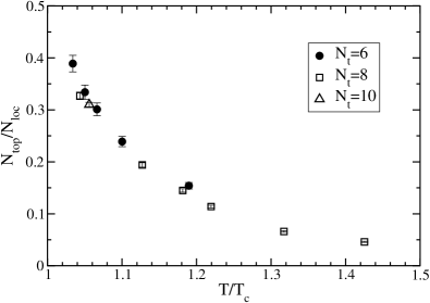
Figure 5: The ratio of the number of instanton zero mode related small eigenvalues to the total number of localized modes as a function of the temperature normalized by the critical temperature. The data sets correspond to lattices with different lattice spacings, namely temporal lattice sizes of $N_{t}=6,8$ and one point for $N_{t}=10$.

VI Conclusions

In the present paper we studied the localization transition in SU(3) Yang-Mills theory. We determined the temperature dependence of the mobility edge, separating localized and delocalized eigenmodes in the Dirac spectrum. By extrapolating the mobility edge as a function of the gauge coupling, we calculated the temperature where the mobility edge reaches zero. At this temperature localized modes completely disappear from the spectrum and for smaller temperatures even the lowest Dirac eigenmodes are delocalized. We found that the temperature where this occurs precisely agrees with the critical temperature of the deconfining phase transition. This indicates that the deconfining and the localization transition are strongly related phenomena. It would be also interesting to understand the details of the physical mechanism of the why these two phenomena are related.

We also identified the part of the Dirac spectrum consisting of close to zero modes produced by instantons and antiinstantons. Just above the transition they account for a bit more than half of the localized modes. However, the fraction of instanton zero mode related localized modes falls sharply with increasing temperature. This comes about from a combination of several effects. On the one hand, with increasing temperature, instantons are squeezed out of the system and their density falls rapidly. On the other hand, the number of localized modes decreases much slower since the decreasing of the spectral density is somewhat compensated by the fact that the mobility edge moves up with increasing temperature. To summarize, even in the quenched theory where the instanton density is higher than in QCD, most of the localized modes cannot be understood as approximate zero modes. It still remains to be seen whether localized modes can be associated to some simply identifiable structure in the gauge field. A first step in this direction might be the finding that localized modes are spatially correlated with local fluctuations in the Polyakov loop Bruckmann:2011cc and the topological charge Cossu:2016scb . Recently it has been found that just above $T_{c}$ the structure of gauge field configurations might be more complicated than a dilute gas of non-interacting instantons Faccioli:2013ja . The possible connection between these recently found dyon structures and localized Dirac eigenmodes is an interesting possibility still to be explored.

References

- (1) S. Borsanyi et al. [Wuppertal-Budapest Collaboration], JHEP 1009, 073 (2010) doi:10.1007/JHEP09(2010)073 [arXiv:1005.3508 [hep-lat]]; A. Bazavov et al., Phys. Rev. D 85, 054503 (2012) doi:10.1103/PhysRevD.85.054503 [arXiv:1111.1710 [hep-lat]].
- (2) J. J. M. Verbaarschot and T. Wettig, Ann. Rev. Nucl. Part. Sci. 50, 343 (2000) [arXiv:hep-ph/0003017].
- (3) A. M. Halász and J. J. M. Verbaarschot, Phys. Rev. Lett. 74, 3920 (1995) [hep-lat/9501025].
- (4) A. M. Garcia-Garcia and J. C. Osborn, Nucl. Phys. A 770, 141 (2006) doi:10.1016/j.nuclphysa.2006.02.011 [hep-lat/0512025].
- (5) A. M. García-García and J. C. Osborn, Phys. Rev. D 75, 034503 (2007) [arXiv:hep-lat/0611019].
- (6) M. Giordano, T. G. Kovacs and F. Pittler, Int. J. Mod. Phys. A 29, no. 25, 1445005 (2014) doi:10.1142/S0217751X14450055 [arXiv:1409.5210 [hep-lat]].
- (7) T. G. Kovács and F. Pittler, Phys. Rev. D 86, 114515 (2012) [arXiv:1208.3475 [hep-lat]].
- (8) M. Giordano, T. G. Kovacs and F. Pittler, Phys. Rev. Lett. 112, no. 10, 102002 (2014) doi:10.1103/PhysRevLett.112.102002 [arXiv:1312.1179 [hep-lat]].
- (9) F. Karsch, E. Laermann and C. Schmidt, Phys. Lett. B 520, 41 (2001) doi:10.1016/S0370-2693(01)01114-5 [hep-lat/0107020]; P. de Forcrand and O. Philipsen, Nucl. Phys. B 673, 170 (2003) doi:10.1016/j.nuclphysb.2003.09.005 [hep-lat/0307020]; P. de Forcrand and O. Philipsen, JHEP 0811, 012 (2008) doi:10.1088/1126-6708/2008/11/012 [arXiv:0808.1096 [hep-lat]].
- (10) M. Giordano, S. D. Katz, T. G. Kovacs and F. Pittler, JHEP 1702, 055 (2017) doi:10.1007/JHEP02(2017)055 [arXiv:1611.03284 [hep-lat]].
- (11) T. Schäfer and E. V. Shuryak, Rev. Mod. Phys. 70, 323 (1998) doi:10.1103/RevModPhys.70.323 [hep-ph/9610451].
- (12) Y. Aoki, Z. Fodor, S. D. Katz and K. K. Szabo, JHEP 0601, 089 (2006) doi:10.1088/1126-6708/2006/01/089 [hep-lat/0510084].
- (13) B.I. Shklovskii, B. Shapiro, B.R. Sears, P. Lambrianides and H.B. Shore, Phys. Rev. B 47 11487 doi.org/10.1103/PhysRevB.47.11487.
- (14) A. Francis, O. Kaczmarek, M. Laine, T. Neuhaus and H. Ohno, Phys. Rev. D 91, no. 9, 096002 (2015) doi:10.1103/PhysRevD.91.096002 [arXiv:1503.05652 [hep-lat]].
- (15) R. Sommer, Nucl. Phys. B 411, 839 (1994) doi:10.1016/0550-3213(94)90473-1 [hep-lat/9310022].
- (16) R. G. Edwards, U. M. Heller, J. E. Kiskis and R. Narayanan, Phys. Rev. D 61, 074504 (2000) doi:10.1103/PhysRevD.61.074504 [hep-lat/9910041].
- (17) A. Alexandru and I. Horváth, Phys. Rev. D 92, no. 4, 045038 (2015) doi:10.1103/PhysRevD.92.045038 [arXiv:1502.07732 [hep-lat]].
- (18) F. Bruckmann, T. G. Kovacs and S. Schierenberg, Phys. Rev. D 84, 034505 (2011) doi:10.1103/PhysRevD.84.034505 [arXiv:1105.5336 [hep-lat]].
- (19) G. Cossu and S. Hashimoto, JHEP 1606, 056 (2016) doi:10.1007/JHEP06(2016)056 [arXiv:1604.00768 [hep-lat]].
- (20) P. Faccioli and E. Shuryak, Phys. Rev. D 87, no. 7, 074009 (2013) doi:10.1103/PhysRevD.87.074009 [arXiv:1301.2523 [hep-ph]]; V. G. Bornyakov, E.-M. Ilgenfritz, B. V. Martemyanov and M. Muller-Preussker, Phys. Rev. D 91, no. 7, 074505 (2015) doi:10.1103/PhysRevD.91.074505 [arXiv:1410.4632 [hep-lat]]; V. Dick, F. Karsch, E. Laermann, S. Mukherjee and S. Sharma, Phys. Rev. D 91, no. 9, 094504 (2015) doi:10.1103/PhysRevD.91.094504 [arXiv:1502.06190 [hep-lat]].