The groupoid of bifractional transformations

Abstract

Bifractional transformations which lead to quantities that interpolate between other known quantities, are considered. They do not form a group, and groupoids are used to described their mathematical structure. Bifractional coherent states and bifractional Wigner functions are also defined. The properties of the bifractional coherent states are studied. The bifractional Wigner functions are used in generalizations of the Moyal star formalism. A generalized Berezin formalism in this context, is also studied.

I Introduction

Phase space methods Z1 ; Z2 are an important part of quantum mechanics. Techniques like fractional Fourier transformsF1 ; F2 ; F3 ; F4 , coherent statesC1 ; C2 ; C3 , analytic representationsB1 ; B2 ; B3 , Wigner and Weyl functions, Moyal formalismM1 ; M2 , Berezin formalismBR1 ; BR2 ; BR3 ; BR4 , etc, provide a deeper understanding of the nature of a quantum particle.

In this paper we introduce bifractional transforms, which lead to new quantities that interpolate between other known quantities. A preliminary version of this has been presented in ALV . Here we go deeper and expand these ideas as follows:

• In section II we review briefly for later use, the mathematical structure of groupoids GR1 ; GR2 ; GR3 ; GR4 . They are weaker but more general than groups. Applications of groupoids in physics include non-commutative geometry A1 ; A2 , quantum tomography A3 , etc.

• In section III we introduce the bifractional displacement operators. They are two-dimensional fractional Fourier transforms, but we stress that they are not a straightforward generalization of the one-dimensional fractional Fourier transforms to the two-dimensional case (a technical point that we explain in section III). The bifractional transformations do not form a group and we use groupoids to describe their mathematical structure. We also study the marginal properties of the bifractional transforms (section III.3).

• In section IV, we act with the bifractional operators on the vacuum, and we get bifractional coherent states. We study their analyticity properties and their resolution of the identity (proposition IV.2). We also study their overlaps and interpret the result in terms of a distance (proposition IV.3). The presentation emphasizes the difference between the formulas for standard coherent states, and the corresponding formulas for the bifractional coherent states.

• In section V we study bifractional Wigner functions $A(\alpha,\beta;\theta_{1},\theta_{2}|\rho)$. Their marginal properties follow immediately from the marginal properties of the bifractional displacement operators in section III.3. In addition to that we give in proposition V.1, extra marginal properties that involve the $|A(\alpha,\beta;\theta_{1},\theta_{2}|\rho)|^{2}$. We also interpret physically the bifractional Wigner functions, as quantities which interpolate between quantum noise and quantum correlations.

• In section VI we present briefly the Moyal star formalism for bifractional Wigner functions (proposition VI.3).

• In section VII we present briefly the corresponding Berezin formalism (proposition VII.2).

II Preliminaries: Groupoid ${\cal T}$ over ${\cal B}$

There are many cases where the concept of group is too strong for the description of a particular symmetry. A weaker concept is the groupoid, which is designed for ‘variable symmetries’. Groups are special cases of groupoids.

A groupoid is a set ${\cal T}$ over a base set ${\cal B}$ such that

• there two maps from ${\cal T}$ to ${\cal B}$

  $$s_{1}(t)=u_{1};\;\;\;s_{2}(t)=u_{2};\;\;\;\;t\in{\cal T};\;\;\;\;u_{1},u_{2}\in{\cal B}$$ (1)

  $u_{1}$ is the ‘source’ of $t$, and $u_{2}$ the ‘target’ of $t$. $t$ can be viewed as an ‘arrow’ which starts at $u_{1}$ and ends at $u_{2}$.

• A partial associative multiplication $t_{1}t_{2}$ is defined only in the case that $s_{2}(t_{1})=s_{1}(t_{2})$ (‘the target of the first arrow is the same as the source of the second arrow’).

• There is an involution (‘inverse’)

  $$t\;\rightarrow\;t^{-1};\;\;\;\;[t^{-1}]^{-1}=t.$$ (2)

• The elements $L_{t}=tt^{-1}$ and $R_{t}=t^{-1}t$ are called left and right identities, and they are in general different. Also

  $$L_{t}t=tR_{t}=t$$ (3)

  Furthermore

  $$s_{1}(t^{-1}t)=s_{2}(t^{-1}t)=s_{1}(t^{-1})=s_{2}(t)$$

  $$s_{1}(tt^{-1})=s_{2}(tt^{-1})=s_{2}(t^{-1})=s_{1}(t).$$ (4)

  The base set ${\cal B}$, is isomorphic to the set of all left identities and to the set of all right identities.

• The set of all elements $t$ such that $s_{1}(t)=s_{2}(t)$ can be shown to form a group, called the isotropy group

In the special case that the base set ${\cal B}$ contains only one element ($L_{t}=R_{t}={\bf 1}$), the multiplication is defined for all elements $t_{1},t_{2}$, and the groupoid is a group. If for all $u_{1},u_{2}\in{\cal B}$ there exists $t\in{\cal T}$ such that $s_{1}(t)=u_{1}$ and $s_{2}(t)=u_{2}$, the groupoid is called connected or transitive.

III Bifractional displacement operators

Let $\hat{x},\hat{p}$ be the position and momentum operators of the harmonic oscillator. We consider the displacement operators

$$D(\alpha,\beta)=\exp(i\sqrt{2}\beta\hat{x}-i\sqrt{2}\alpha\hat{p}),$$ (5)

and the displaced parity operators

$$\Pi(\alpha,\beta) = D\left(\frac{\alpha}{2},\frac{\beta}{2}\right)\Pi(0,0)D^{\dagger}\left(\frac{\alpha}{2},\frac{\beta}{2}\right)$$

$$= D(\alpha,\beta)\Pi(0,0);$$

$$\Pi(0,0) = \int dx\ket{x}\bra{-x}.$$ (6)

They are related through the two-dimensional Fourier transform (e.g., G1 ; G2 ; V1 )

$$\Pi(\alpha,\beta) = \frac{1}{2\pi}\int D(\alpha^{\prime},\beta^{\prime})\exp\left[i(\beta\alpha^{\prime}-\beta^{\prime}\alpha)\right]d\alpha^{\prime}d\beta^{\prime}$$ (7)

$$= \int d\alpha^{\prime}d\beta^{\prime}\Delta\left(\beta,\alpha^{\prime};\frac{\pi}{2}\right)\Delta\left(\alpha,-\beta^{\prime};\frac{\pi}{2}\right)D(\alpha^{\prime},\beta^{\prime})$$

We also consider the fractional Fourier transform:

$$\Delta(x,y;\theta)=\left[\frac{1+i\cot{\theta}}{2\pi}\right]^{1/2}\exp\left[\frac{-i(x^{2}+y^{2})\cot\theta}{2}+\frac{ixy}{\sin\theta}\right]$$ (8)

Special cases of this are

$$\Delta(x,y;0)=\delta(x-y)$$

$$\Delta\left(x,y;\frac{\pi}{2}\right)=\frac{\exp(ixy)}{(2\pi)^{1/2}}$$

$$\Delta(x,y;\pi)=\delta(x+y).$$ (9)

We can prove that

$$\int dy\Delta(x,y;\theta_{1})\Delta(y,z;\theta_{2})=\Delta(x,z;\theta_{1}+\theta_{2}).$$ (10)

In ALV we have generalized Eq.(7) by replacing the Fourier transforms with fractional Fourier transforms. This led to the bifractional displacement operators

$$U(\alpha,\beta;\theta_{1},\theta_{2})=|\cos(\theta_{1}-\theta_{2})|^{\frac{1}{2}}\int d\alpha^{\prime}d\beta^{\prime}\Delta\left(\beta,\alpha^{\prime};\theta_{2}\right)\Delta\left(\alpha,-\beta^{\prime};\theta_{1}\right)D(\alpha^{\prime},\beta^{\prime})$$ (11)

They are unitary operators. The proof of unitarity is based on the integral

$$\int d\alpha^{\prime}d\beta^{\prime}d\alpha^{\prime\prime}d\beta^{\prime\prime}\Delta\left(\beta,\alpha^{\prime};\theta_{2}\right)\Delta\left(\alpha,-\beta^{\prime};\theta_{1}\right)D(\alpha^{\prime},\beta^{\prime})\Delta\left(-\beta,\alpha^{\prime\prime};-\theta_{2}\right)\Delta\left(-\alpha,-\beta^{\prime\prime};-\theta_{1}\right)D(\alpha^{\prime\prime},\beta^{\prime\prime})$$

$$=\frac{{\bf 1}}{|\cos(\theta_{1}-\theta_{2})|}$$ (12)

In order to prove Eq.(III) we use the relation

$$D(\alpha^{\prime},\beta^{\prime})D(\alpha^{\prime\prime},\beta^{\prime\prime})=D(\alpha^{\prime}+\alpha^{\prime\prime},\beta^{\prime}+\beta^{\prime\prime})\exp[i(\beta^{\prime}\alpha^{\prime\prime}-\alpha^{\prime}\beta^{\prime\prime})].$$ (13)

In the integration we are careful with the ordering of operators. The variables $\alpha^{\prime}{},\beta^{\prime}{}$ in Eq.(11), are dual to each other and in this sense our fractional Fourier transform is not a straightforward generalization into two dimensions, of the one-dimensional fractional Fourier transform. Below we give a deeper explanation of the origin of the prefactor $|\cos(\theta_{1}-\theta_{2})|^{\frac{1}{2}}$.

Since $\Delta(x,y;\theta+\pi)=\Delta(x,-y;\theta)$ it follows that

$$U(\alpha,\beta;\theta_{1}+\pi,\theta_{2})=U(-\alpha,\beta;\theta_{1},\theta_{2});\;\;\;\;\;U(\alpha,\beta;\theta_{1},\theta_{2}+\pi)=U(\alpha,-\beta;\theta_{1},\theta_{2})$$ (14)

Therefore we can take $(\theta_{1},\theta_{2})\in{\mathfrak{T}}=[0,\pi)\times[0,\pi)-{\cal L}$, where ${\cal L}$ is the lines $\theta_{1}-\theta_{2}=\pm\frac{\pi}{2}$. We exclude them because in this case the prefactor in Eq.(11) is zero. The following are special cases:

$$U\left(\alpha,\beta;0,0\right)=D(\beta,-\alpha)$$

$$U\left(\alpha,\beta;\frac{\pi}{2},\frac{\pi}{2}\right)=\Pi(\alpha,\beta)$$

$$U\left(\alpha,\beta;\pi,\pi\right)=D(-\beta,\alpha).$$ (15)

III.1 $(\theta_{1},\theta_{2})$ axes in phase space and the origin of the factor $\cos(\theta_{1}-\theta_{2})$

In most of the formulas throughout the paper we get the factor $\cos(\theta_{1}-\theta_{2})$. The following arguments show the Jacobian nature of this factor, and also give a distance used later, in terms of coordinates in a non-orthogonal frame.

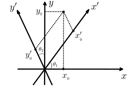
Figure 1: A non-orthogonal frame of $(\theta_{1},\theta_{2})$ axes in phase space

We consider an orthogonal frame $x-y$, and a non-orthogonal frame $x^{\prime}-y^{\prime}$ as shown in fig. 1. The ‘bifractional transform’ in the present context is to rotate the $x$-axis by an angle $\theta_{1}$, and the $y$-axis by an angle $\theta_{2}$, and change variables from $x,y$ to $x^{\prime},y^{\prime}$. Let $(x_{0},y_{0})$ and $(x_{0}^{\prime},y_{0}^{\prime})$ be the coordinates of a point in these two frames, correspondingly. With elementary trigonometry, we express the $(x_{0}^{\prime},y_{0}^{\prime})$ in terms of $(x_{0},y_{0})$ as follows

$$x_{0}^{\prime}=Ax_{0}+By_{0};\;\;\;\;y_{0}^{\prime}=Cx_{0}+Dy_{0}$$ (16)

$$A=\frac{\cos\theta_{2}}{\cos(\theta_{1}-\theta_{2})};\;\;\;\;\;B=\frac{\sin\theta_{2}}{\cos(\theta_{1}-\theta_{2})}$$

$$C=-\frac{\sin\theta_{1}}{\cos(\theta_{1}-\theta_{2})};\;\;\;\;\;D=\frac{\cos\theta_{1}}{\cos(\theta_{1}-\theta_{2})}.$$

Therefore the Jacobian corresponding to this change of variables is

$$\frac{\partial(x_{0}^{\prime},y_{0}^{\prime})}{\partial(x_{0},y_{0})}=AD-BC=\frac{1}{\cos(\theta_{1}-\theta_{2})}.$$ (17)

The distance of the point $(x^{\prime},y^{\prime})$ from the origin is given in terms of the coordinates in the non-orthogonal frame, by

$$[d(x^{\prime},y^{\prime}|\theta_{1},\theta_{2})]^{2}=(x^{\prime})^{2}+(y^{\prime})^{2}+2x^{\prime}y^{\prime}\sin(\theta_{1}-\theta_{2}).$$ (18)

III.2 The groupoid of transformations between the $U(\alpha,\beta;\theta_{1},\theta_{2})$

The bifractional transformations do not form a group under multiplication. It has been shown in ALV that they are elements of the semidirect product of the Heisenberg-Weyl group $HW$ by the $SU(1,1)$ group of squeezing transformations: $HW\rtimes SU(1,1)$. This has general elements of the type

$$S(a_{1},a_{2},a_{3},a_{4},a_{5},a_{6})=\exp[a_{1}\hat{x}^{2}+a_{2}\hat{p}^{2}+a_{3}(\hat{x}\hat{p}+\hat{p}\hat{x})+a_{4}\hat{x}+a_{5}\hat{p}+a_{6}{\bf 1}].$$ (19)

which depend on six parameters. The operators $U(\alpha,\beta;\theta_{\alpha},\theta_{\beta})$ depend only on four parameters, and they are special cases of the operators $S(a_{1},a_{2},a_{3},a_{4},a_{5},a_{6})$.

We describe the mathematical structure of $U(\alpha,\beta;\theta_{1},\theta_{2})$ with groupoids. We consider the set of transformations

$${\cal B}=\{U(\alpha,\beta;\theta_{1},\theta_{2})\};\;\;\;\;(\alpha,\beta;\theta_{1},\theta_{2})\in{\mathbb{R}}\times{\mathbb{R}}\times{\mathfrak{T}}.$$ (20)

We also consider the map

$${T}(\alpha,\beta;\theta_{1},\theta_{2}|\gamma,\delta;\phi_{1},\phi_{2}):U(\alpha,\beta;\theta_{1},\theta_{2})\;\;\rightarrow\;\;U(\gamma,\delta;\phi_{1},\phi_{2}),$$ (21)

where

$$U(\gamma,\delta;\phi_{1},\phi_{2})=\frac{|\cos(\phi_{1}-\phi_{2})|^{\frac{1}{2}}}{|\cos(\theta_{1}-\theta_{2})|^{\frac{1}{2}}}\int d\alpha d\beta\Delta\left(\beta,\delta;\phi_{2}-\theta_{2}\right)\Delta\left(\alpha,\gamma;\phi_{1}-\theta_{1}\right)U(\alpha,\beta;\theta_{1},\theta_{2})$$ (22)

Eq.(22) is a generalized version of Eq.(11), which in the present notation is the map

$${T}{(\alpha^{\prime},\beta^{\prime};0,0|\alpha,\beta;\theta_{1},\theta_{2})}:U(\alpha^{\prime},\beta^{\prime};0,0)\;\;\rightarrow\;\;U(\alpha,\beta;\theta_{1},\theta_{2}),$$ (23)

The compatibility between the two, is shown in the first part of the proof of proposition III.1 below.

We next consider the following notation for the composition

$$[{T}{(\alpha,\beta;\theta_{1},\theta_{2}|\gamma,\delta;\phi_{1}\phi_{2})}\circ{T}{(\gamma,\delta;\phi_{1},\phi_{2}|\epsilon,\zeta;\psi_{1},\psi_{2})}][U(\alpha,\beta;\theta_{1},\theta_{2})]$$

$$={T}{(\gamma,\delta;\phi_{1},\phi_{2}|\epsilon,\zeta;\psi_{1},\psi_{2})}[{T}{(\alpha,\beta;\theta_{1},\theta_{2}|\gamma,\delta;\phi_{1}\phi_{2})}U(\alpha,\beta;\theta_{1},\theta_{2})]$$ (24)

The proposition below shows that the $T(\alpha,\beta;\theta_{1},\theta_{2}|\gamma,\delta;\phi_{1},\phi_{2})$ form a groupoid:

Proposition III.1.

The set $\{{T}{(\alpha,\beta;\theta_{1},\theta_{2}|\gamma,\delta;\phi_{1},\phi_{2})}\}$ is a connected groupoid with base set ${\cal B}$ (in Eq.(20)), and with composition as multiplication. The inverse of ${T}{(\alpha,\beta;\theta_{1},\theta_{2}|\gamma,\delta;\phi_{1},\phi_{2})}$ is

$$[{T}{(\alpha,\beta;\theta_{1},\theta_{2}|\gamma,\delta;\phi_{1},\phi_{2})}]^{-1}={T}{(\gamma,\delta;\phi_{1},\phi_{2}|\alpha,\beta;\theta_{1},\theta_{2})},$$ (25)

The left and right identities are ${T}{(\alpha,\beta;\theta_{1},\theta_{2}|\alpha,\beta;\theta_{1},\theta_{2})}$ and $T(\gamma,\delta;\phi_{1},\phi_{2}|\gamma,\delta;\phi_{1},\phi_{2})$.

Proof.

The proof consists of the following three parts:

• We prove that the following compatibility relation holds

  $${T}{(\alpha,\beta;\theta_{1},\theta_{2}|\gamma,\delta;\phi_{1},\phi_{2})}\circ{T}{(\gamma,\delta;\phi_{1},\phi_{2}|\epsilon,\zeta;\psi_{1},\psi_{2})}={T}{(\alpha,\beta;\theta_{1},\theta_{2}|\epsilon,\zeta;\psi_{1},\psi_{2})}.$$ (26)

  We start with the relations

  $${T}{(\alpha,\beta;\theta_{1},\theta_{2}|\gamma,\delta;\phi_{1},\phi_{2})}[U(\alpha,\beta;\theta_{1},\theta_{2})]=U(\gamma,\delta;\phi_{1},\phi_{2})$$

  $$=\frac{|\cos{(\phi_{1}-\phi_{2})}|^{\frac{1}{2}}}{|\cos{(\theta_{1}-\theta_{2})}|^{\frac{1}{2}}}\int d\alpha d\beta\Delta(\beta,\delta;\phi_{2}-\theta_{2})\Delta(\alpha,\gamma;\phi_{1}-\theta_{1})U(\alpha,\beta;\theta_{1},\theta_{2}),$$ (27)

  and

  $$T(\gamma,\delta;\phi_{1},\phi_{2}|\epsilon,\zeta;\psi_{1},\psi_{2})[U(\gamma,\delta;\phi_{1},\phi_{2})]=U(\epsilon,\zeta;\psi_{1},\psi_{2})$$

  $$=\frac{|\cos{(\psi_{1}-\psi_{2})}|^{\frac{1}{2}}}{|\cos{(\phi_{1}-\phi_{2})}|^{\frac{1}{2}}}\int d\gamma d\delta\Delta(\delta,\zeta;\psi_{2}-\phi_{2})\Delta(\gamma,\epsilon;\psi_{1}-\phi_{1})U(\gamma,\delta;\phi_{1},\phi_{2}).$$ (28)

  Inserting Eq.((1)) into Eq.((1)) we get

  $$T(\gamma,\delta;\phi_{1},\phi_{2}|\epsilon,\zeta;\psi_{1},\psi_{2})[{T}{(\alpha,\beta;\theta_{1},\theta_{2}|\gamma,\delta;\phi_{1},\phi_{2})}[U(\alpha,\beta;\theta_{1},\theta_{2})]]$$

  $$=\frac{|\cos{(\psi_{1}-\psi_{2})}|^{\frac{1}{2}}}{|\cos{(\theta_{1}-\theta_{2})}|^{\frac{1}{2}}}\int d\gamma d\delta\Delta(\delta,\zeta;\psi_{2}-\phi_{2})\Delta(\gamma,\epsilon;\psi_{1}-\phi_{1})$$

  $$\times d\alpha d\beta\Delta(\beta,\delta;\phi_{2}-\theta_{2})\Delta(\alpha,\gamma;\phi_{1}-\theta_{1})U(\alpha,\beta;\theta_{1},\theta_{2}).$$ (29)

  The compatibility relation of Eq.(26) holds because using Eq.(10) we show that Eq.((1)) reduces to

  $$T(\gamma,\delta;\phi_{1},\phi_{2}|\epsilon,\zeta;\psi_{1},\psi_{2})[{T}{(\alpha,\beta;\theta_{1},\theta_{2}|\gamma,\delta;\phi_{1},\phi_{2})}[U(\alpha,\beta;\theta_{1},\theta_{2})]]$$

  $$=\frac{|\cos{(\psi_{1}-\psi_{2})}|^{\frac{1}{2}}}{|\cos{(\theta_{1}-\theta_{2})}|^{\frac{1}{2}}}\int d\alpha d\beta\Delta(\beta,\zeta;\psi_{2}-\theta_{2})\Delta(\alpha,\epsilon;\psi_{1}-\theta_{1})U(\alpha,\beta;\theta_{1},\theta_{2})$$

  $$=T(\alpha,\beta;\theta_{1},\theta_{2}|\epsilon,\zeta;\psi_{1},\psi_{2})[U(\alpha,\beta;\theta_{1},\theta_{2})].$$ (30)

• For the left and right identities, we first point out that in the special case that $\phi_{1}=\theta_{1}$ and $\phi_{2}=\theta_{2}$, the $\Delta\left(\beta,\delta;0\right)$ and $\Delta\left(\alpha,\gamma;0\right)$ are delta functions, and therefore in this case $\alpha=\gamma$ and $\beta=\delta$ and ${T}{(\alpha,\beta;\theta_{1},\theta_{2}|\alpha,\beta;\theta_{1},\theta_{2})}$ is the identity map. We also show that

  $$T(\alpha,\beta;\theta_{1},\theta_{2}|\gamma,\delta;\phi_{1},\phi_{2})\circ{T}{(\gamma,\delta;\phi_{1},\phi_{2}|\alpha,\beta;\theta_{1},\theta_{2})}={T}{(\alpha,\beta;\theta_{1},\theta_{2}|\alpha,\beta;\theta_{1},\theta_{2})}$$

  $${T}{(\gamma,\delta;\phi_{1},\phi_{2}|\alpha,\beta;\theta_{1},\theta_{2})}\circ T(\alpha,\beta;\theta_{1},\theta_{2}|\gamma,\delta;\phi_{1},\phi_{2})={T}{(\gamma,\delta;\phi_{1},\phi_{2}|\gamma,\delta;\phi_{1},\phi_{2})}.$$ (31)

  The inverse, is an involution:

  $$\{[{T}{(\alpha,\beta;\theta_{1},\theta_{2}|\gamma,\delta;\phi_{1},\phi_{2})}]^{-1}\}^{-1}={T}{(\alpha,\beta;\theta_{1},\theta_{2}|\gamma,\delta;\phi_{1},\phi_{2})}.$$ (32)

• The above two parts show that ${\cal T}$ is a groupoid. In fact it is a connected groupoid because any two elements $U(\gamma,\delta;\phi_{1},\phi_{2})$, $U(\alpha,\beta;\theta_{1},\theta_{2})$ in the set ${\cal U}$, are related through Eq.(22).

∎

III.3 Marginal properties for $U(\alpha,\beta;\theta_{1},\theta_{2})$

The proposition below summarizes the marginal properties of $U(\alpha,\beta;\theta_{1},\theta_{2})$:

Proposition III.2.

• Integration of $U(\alpha,\beta;\theta_{1},\theta_{2})$ with respect to $\alpha$ gives

  $$\int d\alpha U(\alpha,\beta;\theta_{1},\theta_{2})=|\cos(\theta_{1}-\theta_{2})|^{\frac{1}{2}}\int d\alpha^{\prime}d\beta^{\prime}\Delta\left(\beta,\alpha^{\prime};\theta_{2}\right)\Delta\left(0,\beta^{\prime};\frac{\pi}{2}-\theta_{1}\right)D(\alpha^{\prime},\beta^{\prime})$$ (33)

• Integration of $U(\alpha,\beta;\theta_{1},\theta_{2})$ with respect to $\beta$ gives

  $$\int d\beta U(\alpha,\beta;\theta_{1},\theta_{2})=|\cos(\theta_{1}-\theta_{2})|^{\frac{1}{2}}\int d\alpha^{\prime}d\beta^{\prime}\Delta\left(0,\alpha^{\prime};\frac{\pi}{2}-\theta_{2}\right)\Delta\left(\alpha,-\beta^{\prime};\theta_{1}\right)D(\alpha^{\prime},\beta^{\prime})$$ (34)

• Integration of $U(\alpha,\beta;\theta_{1},\theta_{2})$ with respect to both $\alpha$ and $\beta$ gives

  $$\int d\alpha d\beta U(\alpha,\beta;\theta_{1},\theta_{2})=U(0,0;\frac{\pi}{2}-\theta_{1},\frac{\pi}{2}-\theta_{2})$$ (35)

Proof.

• $$\int U(\alpha,\beta;\theta_{1},\theta_{2})d\alpha = |\cos(\theta_{1}-\theta_{2})|^{\frac{1}{2}}\left[\frac{1+i\cot\theta_{1}}{2\pi}\right]^{\frac{1}{2}}\int d\alpha^{\prime}d\beta^{\prime}\Delta\left(\beta,\alpha^{\prime};\theta_{2}\right)\exp\left[\frac{-i\beta^{\prime 2}\cot\theta_{1}}{2}\right]D(\alpha^{\prime},\beta^{\prime})$$ (36)

  $$\int d\alpha\exp\left[-\alpha^{2}\left(\frac{i\cot\theta_{1}}{2}\right)-\alpha(\frac{i\beta^{\prime}}{\sin\theta_{1}})\right]$$

  $$= |\cos(\theta_{1}-\theta_{2})|^{\frac{1}{2}}\left[1-i\tan\theta_{1}\right]^{\frac{1}{2}}\int d\alpha^{\prime}d\beta^{\prime}\Delta\left(\beta,\alpha^{\prime};\theta_{2}\right)\exp\left[\frac{i\beta^{\prime 2}\tan\theta_{1}}{2}\right]D(\alpha^{\prime},\beta^{\prime})$$

  $$= |\cos(\theta_{1}-\theta_{2})|^{\frac{1}{2}}\int d\alpha^{\prime}d\beta^{\prime}\Delta\left(\beta,\alpha^{\prime};\theta_{2}\right)\Delta\left(0,\beta^{\prime};\frac{\pi}{2}-\theta_{1}\right)D(\alpha^{\prime},\beta^{\prime})$$

  We have used here the relation

  $$\Delta\left(0,\beta^{\prime};\frac{\pi}{2}-\theta\right)=[1-i\tan\theta]^{\frac{1}{2}}\exp\left[\frac{i\beta^{\prime 2}\tan\theta}{2}\right]$$ (37)

• This is proved in a similar way to the above.

• We integrate Eq.(33) with respect to $\beta$ and we prove Eq.(35).

∎

IV Bifractional coherent states

Acting on the $U(\alpha,\beta;\theta_{1},\theta_{2})$ on the vacuum $\ket{0}$ we get the ’bifractional coherent states’:

$$\ket{\alpha,\beta;\theta_{1},\theta_{2}}=U(\alpha,\beta;\theta_{1},\theta_{2})\ket{0}$$ (38)

We introduce another type of bifractional coherent states, which we call ‘R-bifractional coherent states’, and denote with the index R:

$$\ket{\alpha,\beta;\theta_{1},\theta_{2}}_{R}=U(0,0;\theta_{1},\theta_{2})\ket{\alpha,\beta}$$ (39)

They are eigenstates of the annihilation operator

$$b(\theta_{1},\theta_{2})=U(0,0;\theta_{1},\theta_{2})a[U(0,0;\theta_{1},\theta_{2})]^{\dagger}$$ (40)

and consequently they obey the resolution of the identity

$$\frac{1}{2\pi}\int d\alpha d\beta\ket{\alpha,\beta;\theta_{1},\theta_{2}}_{R\;R}\bra{\alpha,\beta;\theta_{1},\theta_{2}}={\bf 1}.$$ (41)

The proposition below relates the bifractional coherent states in Eqs.(38), (39).

Proposition IV.1.

$$\ket{\alpha,\beta;\theta_{1},\theta_{2}}_{R}=\ket{-\beta\cos\theta_{1}-\alpha\sin\theta_{1},\alpha\cos\theta_{2}-\beta\sin\theta_{2};\theta_{1},\theta_{2}}\exp(iX)$$

$$X=\frac{1}{4}(\beta^{2}-\alpha^{2})[\sin(2\theta_{2})-\sin(2\theta_{1})]+\alpha\beta(\cos^{2}\theta_{1}-\cos^{2}\theta_{2})$$ (42)

Proof.

We will prove that

$$U(0,0;\theta_{1},\theta_{2})D(\alpha,\beta) = U(-\beta\cos\theta_{1}-\alpha\sin\theta_{1},\alpha\cos\theta_{2}-\beta\sin\theta_{2};\theta_{1},\theta_{2})\exp(iX)$$ (43)

We write $U(0,0;\theta_{1},\theta_{2})D(\alpha,\beta)$ as

$$U(0,0;\theta_{1},\theta_{2})D(\alpha,\beta)=|\cos(\theta_{1}-\theta_{2})|^{1/2} \int d\alpha^{\prime}d\beta^{\prime}\exp\left[-\frac{i}{2}(\alpha^{\prime 2}\cot\theta_{2}+\beta^{\prime 2}\cot\theta_{1})\right]$$ (44)

$$\times D(\alpha+\alpha^{\prime},\beta+\beta^{\prime})\exp[i\alpha\beta^{\prime}-i\alpha^{\prime}\beta]$$

Changing variables and combining similar terms we show that,

$$U(0,0;\theta_{1},\theta_{2})\ket{\alpha,\beta}= |\cos(\theta_{1}-\theta_{2})|^{1/2}\exp(iX)\int d\gamma d\lambda\;\;\Delta(\gamma,\alpha\cos\theta_{2}-\beta\sin\theta_{2};\theta_{2})$$ (45)

$$\times\Delta(-\lambda,-\beta\cos\theta_{1}-\alpha\sin\theta_{1};\theta_{1})\ket{\gamma,\lambda}$$

This proves Eq(43) and Eq.(IV.1). ∎

We will use the notation

$$\ket{\alpha,\beta;\theta_{1},\theta_{2}}=\ket{w(\theta_{1},\theta_{2})};\;\;\;\;w(\theta_{1},\theta_{2})=\frac{\alpha e_{2}+i\beta e_{1}}{\cos(\theta_{1}-\theta_{2})}$$

$$e_{2}=i\exp(-i\theta_{2});\;\;\;\;\;e_{1}=i\exp(-i\theta_{1})$$ (46)

$w(\theta_{1},\theta_{2})$ can be written in terms of the $A,B,C,D$ in Eq.(16) as

$$w(\theta_{1},\theta_{2})=\alpha(B+iA)-\beta(D+iC)$$ (47)

$e_{1}$, $e_{2}$ are such that the ‘analyticity part’ of the following proposition, which presents the properties of the bifractional coherent states, holds.

Proposition IV.2.

• [analyticity] The $\exp\left(E(w|w^{*})\right)\ket{w(\theta_{1},\theta_{2})}$, where

  $$E(w|w^{*})=\frac{1}{2}|w|^{2}-\frac{1}{2}b(w^{*})^{2};\;\;\;\;\;b=\frac{1}{4}[\exp(-i2\theta_{1})-\exp(-i2\theta_{2})];\;\;\;\;E(w|w^{*})=[E(w^{*}|w)]^{*}$$ (48)

  depends only on $w$, and does not depend on $w^{*}$.

• [Resolution of the identity]

  $$\frac{1}{2\pi\cos(\theta_{1}-\theta_{2})}\int d\alpha d\beta\ket{\alpha,\beta;\theta_{1},\theta_{2}}\bra{\alpha,\beta;\theta_{1},\theta_{2}}=1$$ (49)

  This can also be written as:

  $$\int\frac{d^{2}w}{2\pi}\ket{w(\theta_{1},\theta_{2})}\bra{w(\theta_{1},\theta_{2})}={\bf 1}$$ (50)

Proof.

• We write the $\exp\left(-\frac{1}{2}b(w^{*})^{2}+\frac{1}{2}|w|^{2}\right)\ket{w(\theta_{1},\theta_{2})}$ as

  $$\exp\left(-\frac{1}{2}b(w^{*})^{2}+\frac{1}{2}|w|^{2}]\right)\ket{w(\theta_{1},\theta_{2})}=|\cos(\theta_{1}-\theta_{2})|^{\frac{1}{2}}\int d^{2}\zeta A(w,\zeta)\exp(\zeta a^{\dagger})\ket{0}$$

  $$A(w,\zeta)=\Delta\left(\mu_{2},\zeta_{R};\theta_{2}\right)\Delta\left(\mu_{1},-\zeta_{I};\theta_{1}\right)\exp\left[-\frac{1}{2}b(w^{*})^{2}+\frac{1}{2}|w|^{2}-\frac{1}{2}|\zeta|^{2}\right]$$

  $$\mu_{1}=\frac{1}{2}(e_{1}^{*}w+e_{1}w^{*})$$

  $$\mu_{2}=\frac{1}{2i}(e_{2}^{*}w-e_{2}w^{*})$$ (51)

  Analyticity of coherent states gives

  $$|\cos(\theta_{1}-\theta_{2})|^{\frac{1}{2}}\int d^{2}\zeta A(w,\zeta)\frac{\partial}{\partial\zeta^{*}}[\exp(\zeta a^{\dagger})\ket{0}]=0.$$ (52)

  and integration by parts gives

  $$|\cos(\theta_{1}-\theta_{2})|^{\frac{1}{2}}\int d^{2}\zeta\left[\frac{\partial}{\partial\zeta^{*}}A(w,\zeta)\right]\exp(\zeta a^{\dagger})\ket{0}=0.$$ (53)

  We will prove that

  $$\frac{\partial}{\partial w^{*}}A(w,\zeta)=\frac{\partial}{\partial\zeta^{*}}A(w,\zeta).$$ (54)

  Eq.(54) gives

  $$\frac{\partial}{\partial w^{*}}A(w,\zeta) = A(w,\zeta)\left[-\frac{i\cot\theta_{2}}{4}(|e_{2}|^{2}w-{e_{2}}^{2}w^{*})-\frac{e_{2}\zeta_{R}}{2\sin\theta_{2}}\right]$$ (55)

  $$+ A(w,\zeta)\left[-\frac{i\cot\theta_{1}}{4}(|e_{1}|^{2}w+e_{1}^{2}w^{*})-\frac{ie_{1}\zeta_{I}}{2\sin\theta_{1}}\right]$$

  $$+ A(w,\zeta)\left(-bw^{*}+\frac{1}{2}w\right)$$

  and also,

  $$\frac{\partial}{\partial\zeta^{*}}A(w,\zeta)= A(w,\zeta)\left[-\frac{ie_{2}\zeta_{R}}{2\sin\theta_{2}}+\frac{1}{4\sin\theta_{2}}(e_{2}^{*}w-e_{2}w^{*})\right]$$ (56)

  $$+A(w,\zeta)\left[-\frac{ie_{1}\zeta_{I}}{2\sin\theta_{1}}+\frac{1}{4\sin\theta_{1}}(e_{1}^{*}w+e_{1}w^{*})\right]$$

  Comparing coefficients we find the values of $e_{1},e_{2}$ given in Eq(IV) and the value of $b$ given in Eq.(48).

  We now insert Eq.(54) into Eq.(53) and prove that

  $$\frac{\partial}{\partial w^{*}}\left[\exp\left(-\frac{1}{2}b(w^{*})^{2}+\frac{1}{2}|w|^{2}\right)\ket{w(\theta_{1},\theta_{2})}\right]=0$$ (57)

• Inserting Eq.(IV.1) into Eq(41) we prove the resolution of identity in Eq.(49). Changing variables from $\alpha,\beta$ to $w(\theta_{1},\theta_{2})$ using Eq.(IV), we prove Eq.(50).

∎

The following proposition, gives the overlap of two bifractional coherent states. The square of the absolute value of this overlap is given in terms of a distance.

Proposition IV.3.

• The overlap of two of these coherent states is

  $$\braket{w(\theta_{1},\theta_{2})}{v(\theta_{1},\theta_{2})} = \exp\left[-\frac{1}{2}|w(\theta_{1},\theta_{2})|^{2}-\frac{1}{2}|v(\theta_{1},\theta_{2})|^{2}+w^{*}(\theta_{1},\theta_{2})v(\theta_{1},\theta_{2})\right]$$ (58)

  $$\times \exp\left[i\left[b^{*}w(\theta_{1},\theta_{2})^{2}+b{w^{*}(\theta_{1},\theta_{2})}^{2}\right]\tan(\theta_{1}-\theta_{2})\right]$$

  $$\times \exp\left[-i\left[b^{*}v(\theta_{1},\theta_{2})^{2}+b{v^{*}(\theta_{1},\theta_{2})}^{2}\right]\tan(\theta_{1}-\theta_{2})\right]$$

  The last two factors are the ‘correction’ to the usual result for the overlap of two coherent states.

• $$|\langle{w(\theta_{1},\theta_{2})}\ket{v(\theta_{1},\theta_{2})}|^{2}=\exp(-|w(\theta_{1},\theta_{2})-v(\theta_{1},\theta_{2})|^{2})=\exp\left\{-\frac{[d(\alpha-\alpha^{\prime},\beta-\beta^{\prime}|\theta_{1},\theta_{2})]^{2}}{\cos^{2}(\theta_{1}-\theta_{2})}\right\}$$ (59)

  Here $d(\alpha-\alpha^{\prime},\beta-\beta^{\prime}|\theta_{1},\theta_{2})$ is the distance discussed in the section III.1. The denominator ${\cos^{2}(\theta_{1}-\theta_{2})}$ is a Jacobian as we change variables from an orthogonal to a non-orthogonal frame. The $w(\theta_{1},\theta_{2})$ and $v(\theta_{1},\theta_{2})$ depend on $\alpha,\beta$ and $\alpha^{\prime}{},\beta^{\prime}{}$ correspondingly, as in Eq.(IV).

Proof.

• We prove Eq.(58) using Eq.(11) for the two bi-fractional operators:

  $$\braket{\alpha,\beta;\theta_{1},\theta_{2}}{\alpha^{\prime},\beta^{\prime};\theta_{1},\theta_{2}}=R\int d\gamma d\lambda d\gamma^{\prime}d\lambda^{\prime}$$

  $$\times\exp\left[-\frac{i}{2}(\gamma^{\prime 2}-\gamma^{2})\cot\theta_{2}+i(\beta\gamma+\beta^{\prime}\gamma^{\prime})\csc\theta_{2}-\frac{i}{2}(\lambda^{\prime 2}-\lambda^{2})\cot\theta_{1}-i(\alpha\lambda+\alpha^{\prime}\lambda^{\prime})\csc\theta_{1}\right]$$

  $$\times\braket{0}{D(\gamma,\lambda)D(\gamma^{\prime},\lambda^{\prime})}{0}$$ (60)

  where,

  $$R=[4\pi^{2}\sin\theta_{1}\sin\theta_{2}]^{-1}\exp{\left[\frac{i}{2}(\alpha^{2}\cot\theta_{1}+\beta^{2}\cot\theta_{2}-\alpha^{\prime 2}\cot\theta_{1}-\beta^{\prime 2}\cot\theta_{2})\right]}$$ (61)

  Then we change notation using Eq.(IV).

• The first part follows immediately from Eq.(58). Then we use Eq.(18) in conjunction with Eq.(IV), and we prove the second part.

∎

V Bifractional Wigner functions: interpolating between quantum noise and quantum correlations

For a density matrix $\rho$ we define the Wigner function $W(\alpha,\beta|\rho)$ and the Weyl function ${\widetilde{W}}(\alpha,\beta|\rho)$ as

$$W(\alpha,\beta|\rho)={\rm Tr}[\rho\Pi(\alpha,\beta)];\;\;\;\;\;{\widetilde{W}}(\alpha,\beta|\rho)={\rm Tr}[\rho D(\alpha,\beta)].$$ (62)

Using Eq.(7) we show that the Wigner and Weyl functions are related through the two-dimensional Fourier transform:

$$W(\alpha,\beta|\rho)=\frac{1}{2\pi}\int{\widetilde{W}}(\alpha^{\prime},\beta^{\prime}|\rho)\exp\left[i(\beta\alpha^{\prime}-\beta^{\prime}\alpha)\right]d\alpha^{\prime}d\beta^{\prime}$$

$$=\int d\alpha^{\prime}d\beta^{\prime}\Delta\left(\beta,\alpha^{\prime};\frac{\pi}{2}\right)\Delta\left(\alpha,-\beta^{\prime};\frac{\pi}{2}\right){\widetilde{W}}(\alpha^{\prime},\beta^{\prime}|\rho).$$ (63)

In ref.ALV we have generalized them into the bifractional Wigner function

$$A(\alpha,\beta;\theta_{1},\theta_{2}|\rho) = {\rm Tr}(\rho U(\alpha,\beta;\theta_{1},\theta_{2})]$$ (64)

$$= |\cos(\theta_{1}-\theta_{2})|^{\frac{1}{2}}\int d\alpha^{\prime}d\beta^{\prime}\Delta\left(\beta,\alpha^{\prime};\theta_{2}\right)\Delta\left(\alpha,-\beta^{\prime};\theta_{1}\right){\widetilde{W}}(\alpha^{\prime},\beta^{\prime}|\rho)$$

In the special case $\theta_{1}=\theta_{2}=0$ this gives the Weyl function

$$A(\alpha,\beta;0,0|\rho)={\widetilde{W}}(\beta,-\alpha|\rho).$$ (65)

In the special case $\theta_{1}=\theta_{2}=\frac{\pi}{2}$ it gives the Wigner function

$$A\left(\alpha,\beta;\frac{\pi}{2},\frac{\pi}{2}|\rho\right)=W(\alpha,\beta|\rho).$$ (66)

Wigner functions quantify the noise, and Weyl functions quantify the correlations in a quantum system. The Weyl function integrates a wavefunction with its displacement in phase space, and in this sense it describes correlations. The widths of the Wigner function describe noise (both quantum and classical) in both the position and momentum. The $\alpha,\beta$ in the Wigner function are position and momentum, while the $\alpha,\beta$ in the Weyl function are position and momentum increments, related to correlations.

The quantity $A(\alpha,\beta;\theta_{1},\theta_{2}|\rho)$ interpolates between the two, and shows that correlations and uncertainties are different aspects of the same concept, which could be called ‘correlation-noise duality’. If $\theta_{1},\theta_{2}$ are close to zero, this more general concept is close to correlations (because $A(\alpha,\beta;\theta_{1},\theta_{2}|\rho)$ is close to the Weyl function), and if $\theta_{1},\theta_{2}$ are close to $\pi/2$, it is close to uncertainties (because $A(\alpha,\beta;\theta_{1},\theta_{2}|\rho)$ is close to the Wigner function). For general values of $\theta_{1},\theta_{2}$ the $A(\alpha,\beta;\theta_{1},\theta_{2}|\rho)$ interpolates between them, and quantifies the noise-correlations duality.

V.1 Marginal properties for $|A(\alpha,\beta;\theta_{1},\theta_{2}|\rho)|^{2}$

In section III.3 we gave the marginal properties for $U(\alpha,\beta;\theta_{1},\theta_{2})$. Taking the trace of both sides of these equations with a density matrix $\rho$, we derive corresponding marginal properties for $A(\alpha,\beta;\theta_{1},\theta_{2}|\rho)$. Below we give marginal properties for $|A(\alpha,\beta;\theta_{1},\theta_{2}|\rho)|^{2}$.

Proposition V.1.

• Integration of $|A(\alpha,\beta;\theta_{1},\theta_{2}|\rho)|^{2}$ with respect to $\alpha$ gives

  $$\int|A(\alpha,\beta;\theta_{1},\theta_{2}|\rho)|^{2}d\alpha = \sqrt{2}\pi|\cos(\theta_{1}-\theta_{2})|$$ (67)

  $$\times \int dx\left\lvert\int d\alpha^{\prime}\Bra{x-\frac{\alpha^{\prime}}{\sqrt{2}}}\rho\Ket{x+\frac{\alpha^{\prime}}{\sqrt{2}}}\Delta\left(\beta,\alpha^{\prime};\theta_{2}\right)\right\rvert^{2}$$

• Integration of $|A(\alpha,\beta;\theta_{1},\theta_{2}|\rho)|^{2}$ with respect to $\beta$ gives

  $$\int|A(\alpha,\beta;\theta_{1},\theta_{2}|\rho)|^{2}d\beta = \sqrt{2}\pi|\cos(\theta_{1}-\theta_{2})|$$ (68)

  $$\times \int dp\left\lvert\int d\beta^{\prime}\Bra{p-\frac{\beta^{\prime}}{\sqrt{2}}}\rho\Ket{p+\frac{\beta^{\prime}}{\sqrt{2}}}\Delta\left(\alpha,-\beta^{\prime};\theta_{1}\right)\right\rvert^{2}$$

• Integration of $|A(\alpha,\beta;\theta_{1},\theta_{2}|\rho)|^{2}$ with respect to both $\alpha$ and $\beta$ gives

  $$\int|A(\alpha,\beta;\theta_{1},\theta_{2}|\rho)|^{2}d\alpha d\beta = \pi|\cos(\theta_{1}-\theta_{2})|{\rm Tr}(\rho^{2})$$ (69)

Proof.

• Using Eq.(64) we get

  $$\int|A(\alpha,\beta;\theta_{1},\theta_{2}|\rho)|^{2}d\alpha = |\cos(\theta_{1}-\theta_{2})|\int d\alpha^{\prime}d\beta^{\prime}\Delta\left(\beta,\alpha^{\prime};\theta_{2}\right)\Delta\left(\alpha,-\beta^{\prime};\theta_{1}\right)\widetilde{W}(\alpha^{\prime},\beta^{\prime}|\rho)$$ (70)

  $$\times \int d\alpha^{\prime\prime}d\beta^{\prime\prime}d\alpha\Delta\left(-\beta,\alpha^{\prime\prime};-\theta_{2}\right)\Delta\left(-\alpha,-\beta^{\prime\prime};-\theta_{1}\right)\widetilde{W}(\alpha^{\prime\prime},\beta^{\prime\prime}|\rho)$$

  Using Eqn.(6), integration with respect to $\alpha$ gives a delta function, and then integration with respect $\beta^{\prime\prime}$ gives

  $$\int|A(\alpha,\beta;\theta_{1},\theta_{2}|\rho)|^{2}d\alpha$$

  $$= |\cos(\theta_{1}-\theta_{2})|\int d\alpha^{\prime}d\alpha^{\prime\prime}d\beta^{\prime}\Delta\left(\beta,\alpha^{\prime};\theta_{2}\right)\Delta\left(-\beta,\alpha^{\prime\prime};-\theta_{2}\right)\widetilde{W}(\alpha^{\prime},\beta^{\prime}|\rho)\widetilde{W}(\alpha^{\prime\prime},-\beta^{\prime}|\rho)$$

  $$= |\cos(\theta_{1}-\theta_{2})|\int d\alpha^{\prime}d\alpha^{\prime\prime}d\beta^{\prime}\Delta\left(\beta,\alpha^{\prime};\theta_{2}\right)\Delta\left(-\beta,\alpha^{\prime\prime};-\theta_{2}\right)$$

  $$\times \int dx\Bra{x-\frac{\alpha^{\prime}}{\sqrt{2}}}\rho\Ket{x+\frac{\alpha^{\prime}}{\sqrt{2}}}\exp(i\sqrt{2}\beta^{\prime}x)\int dy\Bra{y-\frac{\alpha^{\prime\prime}}{\sqrt{2}}}\rho\Ket{y+\frac{\alpha^{\prime\prime}}{\sqrt{2}}}\exp(-i\sqrt{2}\beta^{\prime}y)$$

  Integration with respect to $\beta^{\prime}$ gives a delta function, and changing variables, $x\rightarrow x-\frac{\alpha^{\prime}}{\sqrt{2}}$ and $y\rightarrow y-\frac{\alpha^{\prime\prime}}{\sqrt{2}}$, we get

  $$\int|A(\alpha,\beta;\theta_{1},\theta_{2}|\rho)|^{2}d\alpha=\sqrt{2}\pi|\cos(\theta_{1}-\theta_{2})|\int d\alpha^{\prime}dx\Bra{x-\frac{\alpha^{\prime}}{\sqrt{2}}}\rho\Ket{x+\frac{\alpha^{\prime}}{\sqrt{2}}}\Delta\left(\beta,\alpha^{\prime};\theta_{2}\right)$$

  $$\times\int d\alpha^{\prime\prime}\Bra{x-\frac{\alpha^{\prime\prime}}{\sqrt{2}}}\rho\Ket{x+\frac{\alpha^{\prime\prime}}{\sqrt{2}}}\Delta\left(-\beta,\alpha^{\prime\prime};-\theta_{2}\right)$$

  $$=\sqrt{2}\pi|\cos(\theta_{1}-\theta_{2})|\int dx\left|\int d\alpha^{\prime}\Bra{x-\frac{\alpha^{\prime}}{\sqrt{2}}}\rho\Ket{x+\frac{\alpha^{\prime}}{\sqrt{2}}}\Delta\left(\beta,\alpha^{\prime};\theta_{2}\right)\right|^{2}$$ (72)

• The proof of this is similar to that above

• From Eqs(11),(64) we get

  $$\int|A(\alpha,\beta;\theta_{1},\theta_{2}|\rho)|^{2}d\alpha d\beta =\lambda\int d\alpha d\beta d\alpha^{\prime}d\beta^{\prime}d\alpha^{\prime\prime}d\beta^{\prime\prime}$$

  $$\times\exp\left[\frac{i}{2}(\alpha^{\prime\prime 2}-\alpha^{\prime 2})\cot\theta_{2}+\frac{i}{2}(\beta^{\prime\prime 2}-\beta^{\prime 2})\cot\theta_{1}\right]$$

  $$\times\exp\left[\frac{i\beta(\alpha^{\prime}+\alpha^{\prime\prime})}{\sin\theta_{2}}-\frac{i\alpha(\beta^{\prime}+\beta^{\prime\prime})}{\sin\theta_{1}}\right]{\rm Tr}[\rho D(\alpha^{\prime},\beta^{\prime})]{\rm Tr}[\rho D(\alpha^{\prime\prime},\beta^{\prime\prime})]$$ (73)

  where

  $$\lambda = |\cos(\theta_{1}-\theta_{2})|\left[\frac{1+i\cot{\theta_{1}}}{2\pi}\right]^{1/2}\left[\frac{1-i\cot{\theta_{1}}}{2\pi}\right]^{1/2}\left[\frac{1+i\cot{\theta_{2}}}{2\pi}\right]^{1/2}\left[\frac{1-i\cot{\theta_{2}}}{2\pi}\right]^{1/2}$$ (74)

  $$= \frac{|\cos(\theta_{1}-\theta_{2})|}{4\pi^{2}\sin\theta_{1}\sin\theta_{2}}$$

  Integration over $\alpha,\beta$ gives $\delta$-functions, and then we get Eq.(69).

∎

A special case of Eq.(69) for $\theta_{1}=\theta_{2}=0$ and also $\theta_{1}=\theta_{2}=\frac{\pi}{2}$, is

$$\frac{1}{\pi}\int|W(\alpha,\beta)|^{2}d\alpha d\beta=\frac{1}{\pi}\int|{\widetilde{W}}(\alpha,\beta)|^{2}d\alpha d\beta={\rm Tr}(\rho^{2}).$$ (75)

We next introduce the quantities

$$\langle\langle\alpha^{n}\rangle\rangle=\frac{1}{\pi{\rm Tr}(\rho^{2})}\int\alpha^{n}|A(\alpha,\beta;\theta_{1},\theta_{2}|\rho)|^{2}d\alpha d\beta;\;\;\;\;\delta\alpha(\theta_{1},\theta_{2})=\left[\langle\langle\alpha^{n}\rangle\rangle-(\langle\langle\alpha\rangle\rangle)^{2}\right]^{1/2}$$ (76)

and similarly for $\delta\beta(\theta_{1},\theta_{2})$. Such quantities have been introduced in V for the special case of Wigner and Weyl functions. It has been shown there that for pure states they are the usual uncertainties, but for mixed states they are different. If $\theta_{1},\theta_{2}$ are close to zero, $\delta\alpha(\theta_{1},\theta_{2})$, $\delta\beta(\theta_{1},\theta_{2})$ quantify correlations in position and momentum, and if $\theta_{1},\theta_{2}$ are close to $\pi/2$, they quantify noise.

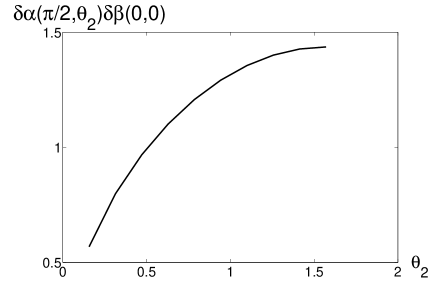
Figure 2: The $\delta\alpha(\frac{\pi}{2},\theta_{2})\delta\beta(0,0)$ as a function of $\theta_{2}$ (in rads), for the density matrix of Eq.(78).

In refV it has been proved that $\delta\alpha(\frac{\pi}{2},\frac{\pi}{2})\delta\beta(0,0)\geq\frac{1}{2}$. In the case of arbitrary angles considered here, we have not proved a similar inequality, but we study this product through an example. As an example, we plot the $\delta\alpha(\frac{\pi}{2},\theta_{2})\delta\beta(0,0)$ as a function of $\theta_{2}$ in fig.2, for the quantum state described with the density matrix

$$\rho=\frac{1}{2}[\ket{\alpha_{0},\beta_{0}}\bra{\alpha_{0},\beta_{0}}+\ket{-\alpha_{0},-\beta_{0}}\bra{-\alpha_{0},-\beta_{0}}];\;\;\;\;\;\ket{\alpha_{0},\beta_{0}}=D(\alpha,\beta)\ket{0};\;\;\;\;\alpha_{0}=2;\;\;\;\;\;\beta_{0}=0.$$ (77)

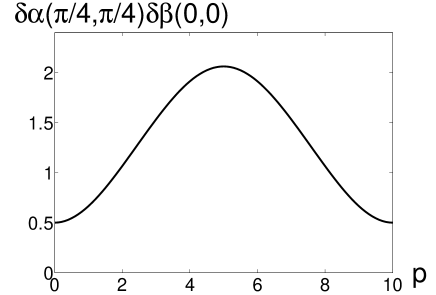
Figure 3: The $\delta\alpha(\frac{\pi}{4},\frac{\pi}{4})\delta\beta(0,0)$ as a function of $p$, for the density matrix of Eq.(78).

We also plot the $\delta\alpha(\frac{\pi}{4},\frac{\pi}{4})\delta\beta(0,0)$ as a function of $p$ in fig.3, for the quantum state described with the density matrix

$$\rho=p\ket{\alpha_{0},\beta_{0}}\bra{\alpha_{0},\beta_{0}}+(1-p)\ket{-\alpha_{0},-\beta_{0}}\bra{-\alpha_{0},-\beta_{0}};\;\;\;\;\;0\leq p\leq 1;\;\;\;\;\alpha_{0}=2;\;\;\;\;\;\beta_{0}=0.$$ (78)

VI Moyal star formalism for bifractional Wigner functions

In this section we present the basic steps of the Moyal formalism for bifractional Wigner functions. We start with a lema which is needed in proofs later.

Lemma VI.1.

For arbitrary states $\ket{\gamma},\ket{\zeta},\ket{\epsilon},\ket{\delta}$

$$\frac{1}{\pi\cos(\theta_{1}-\theta_{2})}\int d\alpha d\beta\braket{\gamma}{U^{\dagger}(\alpha,\beta;\theta_{1},\theta_{2})}{\delta}\braket{\epsilon}{U(\alpha,\beta;\theta_{1},\theta_{2})}{\zeta}=\braket{\gamma}{\zeta}\braket{\epsilon}{\delta}$$ (79)

Proof.

$$\frac{1}{\pi\cos(\theta_{1}-\theta_{2})}\int d\alpha d\beta\braket{\gamma}{U^{\dagger}(\alpha,\beta;\theta_{1},\theta_{2})}{\delta}\braket{\epsilon}{U(\alpha,\beta;\theta_{1},\theta_{2})}{\zeta}$$ (80)

$$= \frac{1}{\pi}\int d\alpha d\beta d\alpha^{\prime}d\beta^{\prime}d\alpha^{\prime\prime}d\beta^{\prime\prime}\bra{\gamma}D(\alpha^{\prime},\beta^{\prime})\ket{\delta}\bra{\epsilon}D(\alpha^{\prime\prime},\beta^{\prime\prime})\ket{\zeta}\Delta(-\beta,\alpha^{\prime};-\theta_{2})\Delta(-\alpha,-\beta^{\prime};-\theta_{1})$$

$$\times \Delta(\beta,\alpha^{\prime\prime};\theta_{2})\Delta(\alpha,-\beta^{\prime\prime};\theta_{1})=\frac{1}{\pi}\int d\alpha^{\prime\prime}d\beta^{\prime\prime}\bra{\gamma}D^{\dagger}(\alpha^{\prime\prime},\beta^{\prime\prime})\ket{\delta}\bra{\epsilon}D(\alpha^{\prime\prime},\beta^{\prime\prime})\ket{\zeta}$$

It is known M1 ; M2 that this is equal to $\braket{\gamma}{\zeta}\braket{\epsilon}{\delta}$. ∎

In the following proposition we express an operator $\Theta$ in terms of the $U(\alpha,\beta;\theta_{1},\theta_{2})$, and the trace of a product of two operators $\Theta_{1}\Theta_{2}$, in terms of the corresponding bifractional Wigner functions.

Proposition VI.2.

• $$\Theta=\frac{1}{\pi\cos(\theta_{1}-\theta_{2})}\int d\alpha d\beta\;\;A^{\dagger}(\alpha,\beta;\theta_{1},\theta_{2}|\Theta)U(\alpha,\beta;\theta_{1},\theta_{2})$$

• $${\rm Tr}(\Theta_{1}\Theta_{2})=\frac{1}{\pi\cos(\theta_{1}-\theta_{2})}\int d\alpha d\beta A(\alpha,\beta;\theta_{1},\theta_{2}|\Theta_{1})A^{\dagger}(\alpha,\beta;\theta_{1},\theta_{2}|\Theta_{2})$$ (82)

Proof.

• $$\frac{1}{\pi\cos(\theta_{1}-\theta_{2})}\int d\alpha d\beta\;\;A^{\dagger}(\alpha,\beta;\theta_{1},\theta_{2}|\Theta)U(\alpha,\beta;\theta_{1},\theta_{2})$$ (83)

  $$=\frac{1}{\pi\cos(\theta_{1}-\theta_{2})}\int d\alpha d\beta\;\;{\rm Tr}[U^{\dagger}(\alpha,\beta;\theta_{1},\theta_{2}|\Theta)]U(\alpha,\beta;\theta_{1},\theta_{2})$$

  $$=\frac{1}{\pi}\int d\alpha d\beta d\alpha^{\prime}d\beta^{\prime}d\alpha^{\prime\prime}d\beta^{\prime\prime}\;\;{\rm Tr}[D^{\dagger}(\alpha^{\prime},\beta^{\prime})\Theta]D(\alpha^{\prime\prime},\beta^{\prime\prime})\Delta(-\beta,\alpha^{\prime};-\theta_{2})\Delta(-\alpha,-\beta^{\prime};-\theta_{1})$$

  $$\times \Delta(\beta,\alpha^{\prime\prime};\theta_{2})\Delta(\alpha,-\beta^{\prime\prime};\theta_{1})=\frac{1}{\pi}\int d\alpha d\beta\;\;{\rm Tr}[D^{\dagger}(\alpha,\beta)\Theta]D(\alpha,\beta)=\Theta$$

  The last equality is a known relation (e.g., V1 ).

  A second proof based on lemma VI.1, is to consider the matrix elements of both sides with ordinary coherent states $\ket{z}$, $\ket{w}$:

  $$\bra{z}\Theta\ket{w}=\frac{1}{\pi\cos(\theta_{1}-\theta_{2})}\int d\alpha d\beta\;\;A^{\dagger}(\alpha,\beta;\theta_{1},\theta_{2}|\Theta)\bra{z}U(\alpha,\beta;\theta_{1},\theta_{2})\ket{w}$$

  Also

  $$A^{\dagger}(\alpha,\beta;\theta_{1},\theta_{2}|\Theta)={\rm Tr}[\Theta U^{\dagger}(\alpha,\beta;\theta_{1},\theta_{2})]=\int\frac{d^{2}z}{\pi}\frac{d^{2}u}{\pi}\bra{\zeta}\theta\ket{u}\bra{u}U^{\dagger}(\alpha,\beta;\theta_{1},\theta_{2})\ket{\zeta}$$ (85)

  Combining Eqs.((1)),(85) and using lemma VI.1, which is valid for arbitrary states and therefore for coherent states, we prove Eq.((1)).

• Using Eq.(64) we get

  $$\frac{1}{\pi\cos(\theta_{1}-\theta_{2})}\int d\alpha d\beta A(\alpha,\beta;\theta_{1},\theta_{2}|\Theta_{1})A^{\dagger}(\alpha,\beta;\theta_{1},\theta_{2}|\Theta_{2})$$ (86)

  $$= \frac{1}{\pi\cos(\theta_{1}-\theta_{2})}\int d\alpha^{\prime}d\beta^{\prime}d\alpha^{\prime\prime}d\beta^{\prime\prime}\widetilde{W}(\alpha^{\prime},\beta^{\prime}|\Theta_{1})\widetilde{W}(\alpha^{\prime\prime},\beta^{\prime\prime}|\Theta_{2})$$

  $$\times \Delta(-\beta,\alpha^{\prime};-\theta_{2})\Delta(-\alpha,-\beta^{\prime};-\theta_{1})\Delta(\beta,\alpha^{\prime\prime};\theta_{2})\Delta(\alpha,-\beta^{\prime\prime};\theta_{1})$$

  Using Eq.(10) we get delta functions, which give

  $$= \frac{1}{\pi}\int d\alpha^{\prime\prime}d\beta^{\prime\prime}\;\widetilde{W}(-\alpha^{\prime\prime},-\beta^{\prime\prime}|\Theta_{1})\widetilde{W}(\alpha^{\prime\prime},\beta^{\prime\prime}|\Theta_{2})$$ (87)

  $$= \frac{1}{\pi}\int d\alpha^{\prime\prime}d\beta^{\prime\prime}\;\Braket{x+\frac{\alpha^{\prime\prime}}{\sqrt{2}}}{\Theta_{1}}{x-\frac{\alpha^{\prime\prime}}{\sqrt{2}}}\Braket{y-\frac{\alpha^{\prime\prime}}{\sqrt{2}}}{\Theta_{2}}{x+\frac{\alpha^{\prime\prime}}{\sqrt{2}}}e^{i\sqrt{2}\beta^{\prime\prime}(y-x)}$$

  Integrating with respect to $\beta^{\prime\prime}$, and changing variables, we show that:

  $$= \sqrt{2}\int d\alpha^{\prime\prime}dx\;\Braket{x+\frac{\alpha^{\prime\prime}}{\sqrt{2}}}{\Theta_{1}}{x-\frac{\alpha^{\prime\prime}}{\sqrt{2}}}\Braket{x-\frac{\alpha^{\prime\prime}}{\sqrt{2}}}{\Theta_{1}}{x+\frac{\alpha^{\prime\prime}}{\sqrt{2}}}$$ (88)

  $$= \int dk\braket{k}{\Theta_{1}\Theta_{2}}{k}={\rm Tr}[\Theta_{1}\Theta_{2}].$$

∎

Given the $A(\alpha,\beta;\theta_{1},\theta_{2}|\Theta_{1})$ and $A(\alpha,\beta;\theta_{1},\theta_{2}|\Theta_{2})$ of two operators $\Theta_{1},\Theta_{2}$, the following proposition gives the $A(\alpha,\beta;\theta_{1},\theta_{2}|\Theta_{1}\Theta_{2})$ of their product.

Proposition VI.3.

$$A(\epsilon,\zeta;\theta_{1},\theta_{2}|\Theta_{1}\Theta_{2})$$ (89)

$$=\frac{1}{\pi[\cos(\theta_{1}-\theta_{2})]^{1/2}}\int d\alpha^{\prime}d\beta^{\prime}d\alpha\;d\beta\;d\gamma\;d\lambda\;d\gamma^{\prime}\;d\lambda^{\prime}\;A^{\dagger}(\alpha,\beta;\theta_{1},\theta_{2}|\Theta_{1})\;A^{\dagger}(\alpha^{\prime},\beta^{\prime};\theta_{1},\theta_{2}|\Theta_{2})$$

$$\times \Delta(\beta,\gamma;\theta_{2})\Delta(\alpha,-\lambda;\theta_{1})\Delta(\beta^{\prime},\gamma^{\prime};\theta_{2})\Delta(\alpha^{\prime},-\lambda^{\prime};\theta_{1})\Delta(\zeta,-(\gamma+\gamma^{\prime});\theta_{2})\Delta(\epsilon,\lambda+\lambda^{\prime};\theta_{1})$$

$$\times\exp[i\lambda\gamma^{\prime}-i\gamma\lambda^{\prime}]$$

Proof.

Eq.(64) gives

$$A(\epsilon,\zeta;\theta_{1},\theta_{2}|\Theta_{1}\Theta_{2})=|\cos(\theta_{1}-\theta_{2})|^{1/2}\int d\epsilon^{\prime}\;d\zeta^{\prime}\;\Delta(\zeta,\epsilon^{\prime};\theta_{2})\Delta(\epsilon,-\zeta^{\prime};\theta_{1})\;{\rm Tr}[D(\epsilon^{\prime},\zeta^{\prime})\Theta_{1}\Theta_{2}]$$ (90)

Using Eq.((1)) we get

$$\Theta_{1}\Theta_{2} = \frac{1}{[\pi\cos(\theta_{1}-\theta_{2})]^{2}}\int d\alpha^{\prime}d\beta^{\prime}d\alpha d\beta\;A^{\dagger}(\alpha,\beta;\theta_{1},\theta_{2}|\Theta_{1})\;A^{\dagger}(\alpha^{\prime},\beta^{\prime};\theta_{1},\theta_{2}|\Theta_{2})$$ (91)

$$\times \;U(\alpha,\beta;\theta_{1},\theta_{1})\;U(\alpha^{\prime},\beta^{\prime};\theta_{1},\theta_{2})$$

Therefore

$$A(\epsilon,\zeta;\theta_{1},\theta_{2}|\Theta_{1}\Theta_{2}) = \frac{[{\cos(\theta_{1}-\theta_{2})}]^{-3/2}}{\pi^{2}}\int d\alpha^{\prime}d\beta^{\prime}d\alpha d\beta\;d\epsilon^{\prime}d\zeta^{\prime}A^{\dagger}(\alpha,\beta;\theta_{\alpha},\theta_{\beta}|\Theta_{1})\;A^{\dagger}(\alpha^{\prime},\beta^{\prime};\theta_{1},\theta_{2}|\Theta_{2})$$ (92)

$$\times {\rm Tr}[U(\alpha,\beta;\theta_{1},\theta_{2})U(\alpha^{\prime},\beta^{\prime};\theta_{1},\theta_{2})D(\epsilon^{\prime},\zeta^{\prime})]\Delta(\zeta,\epsilon^{\prime};\theta_{2})\Delta(\epsilon,-\zeta^{\prime};\theta_{1})$$

$$= \frac{[{\cos(\theta_{1}-\theta_{2})}]^{-3/2}}{\pi^{2}}\int d\alpha^{\prime}d\beta^{\prime}d\alpha d\beta\;d\epsilon^{\prime}d\zeta^{\prime}d\gamma\;d\lambda\;d\gamma^{\prime}\;d\lambda^{\prime}\;A^{\dagger}(\alpha,\beta;\theta_{1},\theta_{2}|\Theta_{1})\;$$

$$\times A^{\dagger}(\alpha^{\prime},\beta^{\prime};\theta_{1},\theta_{2}|\Theta_{2})\Delta(\beta,\gamma;\theta_{2})\Delta(\alpha,-\lambda;\theta_{1})\Delta(\beta^{\prime},\gamma^{\prime};\theta_{2})\Delta(\alpha^{\prime},-\lambda^{\prime};\theta_{1})$$

$$\times {\rm Tr}[D(\gamma,\lambda)D(\gamma^{\prime},\lambda^{\prime})D(\epsilon^{\prime},\zeta^{\prime})]\Delta(\zeta,\epsilon^{\prime};\theta_{2})\Delta(\epsilon,-\zeta^{\prime};\theta_{1})$$

But

$${\rm Tr}[D(\gamma,\lambda)D(\gamma^{\prime},\lambda^{\prime})D(\epsilon^{\prime},\zeta^{\prime})]=\pi\delta(\epsilon^{\prime}+\gamma+\gamma^{\prime})\delta(\zeta^{\prime}+\lambda+\lambda^{\prime})\exp[i(\lambda\gamma^{\prime}-\gamma\lambda^{\prime})].$$ (93)

Inserting this in Eq.(92) we prove the proposition. ∎

VII Generalized Berezin formalism

The Berezin formalismBR1 ; BR2 ; BR3 ; BR4 represents an operator $\Theta$ with the analytic function $L(z,w^{*};\theta_{1},\theta_{2}|\Theta)$ defined below. It shows that the $L(z,z^{*};\theta_{1},\theta_{2}|\Theta_{1}\Theta_{2})$ of the product of two operators $\Theta_{1}\Theta_{2}$, can be expanded as a Taylor series, where the first term is the product $L(z,z^{*};\theta_{1},\theta_{2}|\Theta_{1})L(z,z^{*};\theta_{1},\theta_{2}|\Theta_{2})$ (which is classical in the sense that it is commutative), and the other terms are quantum corrections (and go to zero in the limit $\hbar\rightarrow 0$). The Laplacian used in the standard Berezin formalism, is replaced here with the ‘bifractional Laplacian’ defined below.

Lemma VII.1.

For $K>0$

$$\frac{1}{2\pi\cos(\theta_{1}-\theta_{2})}\int d\alpha^{\prime}d\beta^{\prime}F(\alpha^{\prime},\beta^{\prime})K\exp\left\{-\frac{K[d(\alpha-\alpha^{\prime},\beta-\beta^{\prime}|\theta_{1},\theta_{2})]^{2}}{\cos^{2}(\theta_{1}-\theta_{2})}\right\}$$

$$=\frac{1}{2}\left[\exp{\left(\frac{\Delta_{(\alpha,\beta|\theta_{1},\theta_{2})}}{4K}\right)}F(\alpha,\beta)\right],$$ (94)

where

$$\Delta_{(\alpha,\beta|\theta_{1},\theta_{2})}=\frac{\partial^{2}}{\partial^{2}\alpha}+\frac{\partial^{2}}{\partial^{2}\beta}-2\frac{\partial^{2}}{\partial\alpha\partial\beta}\sin(\theta_{1}-\theta_{2}).$$ (95)

If we replace $\alpha^{\prime}{},\beta^{\prime}{}$ with $w,w^{*}$ given in Eq.(IV) (and $\alpha,\beta$ with $z,z^{*}$), then Eq.(95) can be re-written as

$$\frac{1}{2\pi}\int d^{2}wF(w,w^{*})K\exp{\left[-K{|w(\theta_{1},\theta_{2})-z(\theta_{1},\theta_{2})|}^{2}\right]}=\frac{1}{2}\left[\exp{\left(\frac{\Delta_{(z,z^{*}|\theta_{1},\theta_{2})}}{4K}\right)}F(z,z^{*})\right],$$ (96)

where $\Delta_{(z,z^{*}|\theta_{1},\theta_{2})}$ is the ‘bifractional Laplacian’

$$\Delta_{(z,z^{*}|\theta_{1},\theta_{2})}=4\frac{\partial^{2}}{\partial z\partial z^{*}}-2i\left[\frac{\partial^{2}}{\partial^{2}z}-\frac{\partial^{2}}{\partial^{2}z^{*}}\right]\sin(\theta_{1}-\theta_{2}).$$ (97)

Proof.

The proof of Eq.(VII.1) is based on a Fourier transform of both sides (it is lengthy but straightforward).

∎

Let

$$L(z,w^{*};\theta_{1},\theta_{2}|\Theta)=\exp\left[\frac{1}{2}|z|^{2}+\frac{1}{2}|w|^{2}-zw^{*}\right]\braket{z^{*}(\theta_{1},\theta_{2})}{\Theta}{w^{*}(\theta_{1},\theta_{2})}$$ (98)

This is an analytic function of $w^{*}(\theta_{1},\theta_{2})$ and $z(\theta_{1},\theta_{2})$.

Proposition VII.2.

$$L(z,z^{*};\theta_{1},\theta_{2}|\Theta_{1}\Theta_{2})=\frac{1}{2}\left[\exp{\left(\frac{\Delta_{(\zeta,\zeta^{*}|\theta_{1},\theta_{2})}}{4}\right)}L(z,\zeta^{*};\theta_{1},\theta_{2}|\Theta_{1})L(\zeta,z^{*};\theta_{1},\theta_{2}|\Theta_{2})\right]_{\zeta=z}$$ (99)

Taylor expansion gives

$$L(z,z^{*};\theta_{1},\theta_{2}|\Theta_{1}\Theta_{2}) = L(z,z^{*};\theta_{1},\theta_{2}|\Theta_{1})L(z,z^{*};\theta_{1},\theta_{2}|\Theta_{2})$$ (100)

$$+\frac{\partial L(z,z^{*};\theta_{1},\theta_{2}|\Theta_{1})}{2\partial z^{*}}\frac{\partial L(z,z^{*};\theta_{1},\theta_{2}|\Theta_{1})}{\partial z}$$

$$+\left[i\sin(\theta_{1}-\theta_{2})\frac{\partial^{2}L(z,z^{*};\theta_{1},\theta_{2}|\Theta_{1})L(z,z^{*};\theta_{1},\theta_{2}|\Theta_{2})}{4\partial^{2}z^{*}}\right]$$

$$-\left[i\sin(\theta_{1}-\theta_{2})\frac{\partial^{2}L(z,z^{*};\theta_{1},\theta_{2}|\Theta_{1})L(z,z^{*};\theta_{1},\theta_{2}|\Theta_{2})}{4\partial^{2}z}\right]+...$$

Proof.

For two arbitrary operators $\Theta_{1},\Theta_{2}$ we have that,

$$L(z,z^{*};\theta_{1},\theta_{2}|\Theta_{1}\Theta_{2})=\int d^{2}wD_{E}(z,w;\theta_{1},\theta_{2})L(z,w^{*};\theta_{1},\theta_{2}|\Theta_{1})L(w,z^{*};\theta_{1},\theta_{2}|\Theta_{2})$$

$$D_{E}(z,w;\theta_{1},\theta_{2})=|\langle{z(\theta_{1},\theta_{2})}\ket{w(\theta_{1},\theta_{2})}|^{2}$$ (101)

Then using Eq.(96), we prove Proposition VII.2. ∎

VIII Discussion

We have studied bifractional transforms, and their application in the area of phase space methods. They provide a two-parameter ($\theta_{1},\theta_{2}$) interpolation between other known quantities. We have explained that they do not form a group and we used groupoids to describe their mathematical structure.

The work generalizes the traditional concept of phase space. The Wigner function $W(\alpha,\beta)$ describes the quantum noise in the position of a particle in the phase space $\alpha-\beta$. The Weyl function describes quantum correlations in the space $\alpha^{\prime}-\beta^{\prime}$ of position and momentum increments. $(\alpha,\beta^{\prime})$ are dual variables in the Fourier transform sense, and the same is true for $(\alpha^{\prime},\beta)$. Through fractional Fourier transforms, we work in an intermediate phase space $\alpha_{\theta_{1}}-\beta_{\theta_{2}}$, where $\alpha_{\theta_{1}}$ is in the plane $\alpha-\beta^{\prime}$, and $\beta_{\theta_{2}}$ is in the plane $\alpha^{\prime}\boldsymbol{-}\beta$. When $\theta_{1}=\theta_{2}=0$, the $\alpha_{\theta_{1}}-\beta_{\theta_{2}}$ is the $\alpha-\beta$ position-momentum phase space, associated with the Wigner function and quantum noise. When $\theta_{1}=\theta_{2}=\frac{\pi}{2}$, the $\alpha_{\theta_{1}}-\beta_{\theta_{2}}$ is the dual phase space $\alpha^{\prime}-\beta^{\prime}$ of position increment and momentum increment, associated with the Weyl function and quantum correlations. Our intermediate phase space is related to novel intermediate quantities between quantum correlations and quantum noise, and reveals deep links between them.

Using bifractional transforms we have defined bifractional coherent states. Their analyticity properties and their resolution of the identity have been presented in proposition IV.2. They are the counterparts in the phase space $\alpha_{\theta_{1}}-\beta_{\theta_{2}}$, of the standard coherent states in the phase space $\alpha-\beta$.

We have also defined bifractional Wigner functions $A(\alpha,\beta;\theta_{1},\theta_{2}|\rho)$. We have studied their properties, and interpreted them physically as quantities which interpolate between quantum noise and quantum correlations. We have also studied the Moyal star formalism for bifractional Wigner functions, and the corresponding Berezin formalism (proposition VII.2). This provides a complete study of the $\alpha_{\theta_{1}}-\beta_{\theta_{2}}$ phase space that we introduced in this paper.

References

- (1) C.K. Zachos, D.B. Fairlie, T.L. Curtright, ‘Quantum Mechanics in Phase Space’ (World Scientific, Singapore, 2005)
- (2) W.P. Schleich, ‘Quantum Optics in Phase Space’, (Wiley, New York, 2001)
- (3) V. Namias, J. Inst. Math. Applic., 25, 241, (1980).
- (4) A. C. McBride, F. H. Kerr, IMA J. Appl. Math., 39, 159, (1987).
- (5) D. H. Bailey, P. N. Swarztrauber, SIAM Review, 33, 389, (1991).
- (6) H. M. Ozaktas, Z. Zalevsky, M.A. Kutay, ‘The Fractional Fourier Transform’ (Wiley, New York, 2001)
- (7) J.R. Klauder, B-S. Skagerstam, ‘Coherent states’ (World Scientific, Singapore, 1985)
- (8) A. Perelomov, ‘Generalized coherent states and their applications’ (Springer, Berlin, 1986)
- (9) A.S Twareque, J-P Antonie, J-P Gazeau, ‘Coherent states, Wavelets, and Their Generalizations’ (Springer, Berlin, 2000)
- (10) V. Bargmann, Comm. Pure Appl. Math. 14, 180 (1961)
- (11) B.C. Hall, Contemp. Math. 260, 1 (2000)
- (12) A. Vourdas, J. Phys. A39, R65 (2006)
- (13) J.E. Moyal, Proc. Cambridge Philos. Soc. 45, 99 (1949)
- (14) M.S. Bartlett, J. E. Moyal, Proc. Cambridge Philos. Soc. 45, 545 (1949)
- (15) F.A. Berezin, Math. USSR Izv. 8, 1109 (1974)
- (16) F.A. Berezin, Math. USSR Izv. 9, 341 (1975)
- (17) F.A. Berezin, Comm. Math. Phys. 40, 153 (1975)
- (18) F.A. Berezin, Sov. Math. Dokl. 19, 786 (1978)
- (19) S. Agyo, C. Lei, A. Vourdas, Phys. Lett. A379, 255 (2015)
- (20) A. Weinstein, Notices of the Am. Math. Soc. 43, 744 (1996)
- (21) M.V. Karasev, Math. USSR Izvestia, 28, 497 (1978)
- (22) R. Brown, Bull. London Math. Soc. 19, 113 (1987)
- (23) C.M. Marle in Encyclopedia Math. Phys. p.312 (Elsevier, Amsterdam, 2006)
- (24) A. Connes, ‘Non-commutative geometry’ (Academic Press, London, 1994)
- (25) N.P. Landsman, J. Geom. Phys. 56, 24 (2006)
- (26) A. Ibort, V.I. Manko, G. Marmo, A. Simoni, C. Stornaiolo, F. Vertinglia, Phys. Scripta, 88, 055003 (2013)
- (27) A.Grossmann Commun. Math. Phys. 48, 191 (1976)
- (28) A.Royer Phys. Rev. A45, 793 (1992)
- (29) R. F. Bishop, A. Vourdas, Phys. Rev. A, 50, 4488, (1994)
- (30) A. Vourdas, Phys. Rev. A69, 022108 (2004)