Testing Isotropic Universe Using the Gamma-Ray Burst
Data of Fermi / GBM

Abstract

The sky distribution of Gamma-Ray Bursts (GRBs) has been intensively studied by various groups for more than two decades. Most of these studies test the isotropy of GRBs based on their sky number density distribution. In this work we propose an approach to test the isotropy of the Universe through inspecting the isotropy of the properties of GRBs such as their duration, fluences and peak fluxes at various energy bands and different time scales. We apply this method on the Fermi / Gamma-ray Burst Monitor (GBM) data sample containing 1591 GRBs. The most noticeable feature we found is near the Galactic coordinates $l\approx 30^{\circ}$, $b\approx 15^{\circ}$ and radius $r\approx 20^{\circ}-40^{\circ}$. The inferred probability for the occurrence of such an anisotropic signal (in a random isotropic sample) is derived to be less than a percent in some of the tests while the other tests give results consistent with isotropy. These are based on the comparison of the results from the real data with the randomly shuffled data samples. Considering large number of statistics we used in this work (which some of them are correlated to each other) we can anticipate that the detected feature could be result of statistical fluctuations. Moreover, we noticed a considerably low number of GRBs in this particular patch which might be due to some instrumentation or observational effects that can consequently affect our statistics through some systematics. Further investigation is highly desirable in order clarify about this result, e.g. utilizing a larger future Fermi / GBM data sample as well as data samples of other GRB missions and also looking for possible systematics.

1 Introduction

Recent observations claimed the existence of large-scale structures in the Universe of sizes of several hundreds of megaparsecs or even beyond one gigaparsec. For example the Sloan Great Wall of galaxies (Gott et al., 2005) 419 Mpc long at redshift $z=0.073$ has been reported. The radio observations of the National Radio Astronomy Observatory’s Very Large Array Sky Survey suggested a 140 Mpc completely empty void at $z\leq 1$ (Rudnick et al., 2007). Or a Huge Large Quasar Group (Huge-LQG) of longest dimension $\sim 1240$ Mpc at mean redshift $\bar{z}=1.27$ has been claimed (Clowes et al., 2013). However, Nadathur (2013) argued that interpreting the Huge-LQG as a structure is questionable.

Concerning the Gamma-Ray Bursts (GRBs) (Vedrenne & Atteia, 2009; Kouveliotou et al., 2012; Kumar & Zhang, 2015), initially they had been claimed to be distributed isotropically on the sky (Meegan et al., 1992; Briggs et al., 1996; Tegmark et al., 1996). Later several works claimed that short GRBs ($T_{90}<2$ s) were distributed anisotropically (Balázs et al., 1998, 1999; Magliocchetti et al., 2003; Vavrek et al., 2008; Tarnopolski, 2017), where $T_{90}$ is the duration during which 90 % of the detected counts from a GRB is accumulated (Kouveliotou et al., 1993). However, Mészáros et al. (2000a, b); Litvin et al. (2001); Bernui et al. (2008); Veres et al. (2010a); Ukwatta & Woźniak (2016) claimed different results. The pertinent intermediate-duration GRBs (2 s $\lesssim T_{90}\lesssim$ 10 s) (Mukherjee et al., 1998; Horváth, 1998; Balastegui et al., 2001; Horváth, 2002; Horváth et al., 2008; Horváth, 2009; Huja et al., 2009; Řípa et al., 2009; Horváth et al., 2010; Veres et al., 2010b; de Ugarte Postigo et al., 2011; Řípa et al., 2012; Zitouni et al., 2015; Horváth & Tóth, 2016; Řípa & Mészáros, 2016; Yang et al., 2016; Kulkarni & Desai, 2017) were found to be distributed anisotropically on the sky (Mészáros et al., 2000a, b; Litvin et al., 2001; Vavrek et al., 2008; Veres et al., 2010a). However, Mészáros & Štoček (2003); Ukwatta & Woźniak (2016) claimed different results. It was also found that very short GRBs ($T_{90}\leq 100$ ms) were distributed anisotropically (Cline et al., 2005; Ukwatta & Woźniak, 2016). Long GRBs ($T_{90}>2$ s) were proclaimed to be distributed isotropically (Balázs et al., 1998, 1999; Mészáros et al., 2000a, b; Magliocchetti et al., 2003; Vavrek et al., 2008; Tarnopolski, 2017; Ukwatta & Woźniak, 2016), however Mészáros & Štoček (2003) claimed different result. For review of these works see Mészáros et al. (2009a, b); Mészáros (2017).

Recently, Horváth et al. (2014, 2015) studied the spatial distribution of GRBs taking into account their redshift. They concluded that there was a statistically significant clustering of GRBs at redshift $1.6<z\leq 2.1$ and that the size of the structure defined by these GRBs was about 2 000–3 000 Mpc, so called Hercules–Corona Borealis Great Wall. Contrary to this, Ukwatta & Woźniak (2016) claimed that their redshift-dependent analysis did not provide evidence of significant clustering. A discussion of the implications of the results obtained by Horváth et al. (2014) on the Cosmological Principle can be found in Li & Lin (2015).

Balázs et al. (2015) reported the discovery of a giant ring-like structure with a diameter of 1 720 Mpc, displayed by 9 GRBs. The ring has a major diameter of $43^{\circ}$ and a minor diameter of $30^{\circ}$ at a distance of 2 770 Mpc in the redshift range of $0.78<z<0.86$.

Another work testing the isotropic distribution of GRBs and making a comparison with Cosmic Microwave Background (CMB) can be found in Gan et al. (2016).

Further information about the tests of the isotropy or homogeneity of the Universe using SNe Ia, CMB, dark energy, galaxies and large-scale structures see, e.g. Hinshaw et al. (1996); Frith et al. (2005a, b); Hogg et al. (2005); Campanelli et al. (2011); Colin et al. (2011); Scrimgeour et al. (2012); Feindt et al. (2013); Appleby & Shafieloo (2014); Fernández-Cobos et al. (2014); Planck Collaboration et al. (2014); Appleby et al. (2015); Javanmardi et al. (2015); Planck Collaboration et al. (2016); Chen & Chen (2017); Javanmardi & Kroupa (2017) and references therein.

All these studies, which use GRB data, test the isotropy based on the distribution of the number densities of GRBs. On the other hand, in this paper we test the isotropy of the Universe through inspecting the isotropy of the properties of GRBs such as their duration, fluences and peak fluxes at various energy bands and different time scales.

The paper is organized as follows. Section 2 describes the used data sample. Section 3 details the proposed methodology. The results are presented in Section 4 and in Appendix A. Our findings are discussed in Section 5 and Section 6 summarizes the conclusions.

2 Data Sample

The database of the Fermi satellite (Atwood & GLAST Collaboration, 1994) and particularly of the Gamma-ray Burst Monitor (GBM) instrument (Meegan et al., 2009) has been utilized in this work. Specifically we employed the FERMIGBRST - Fermi GBM Burst Catalog (Gruber et al., 2014; von Kienlin et al., 2014; Narayana Bhat et al., 2016), which is being constantly updated. While methods for measuring GRB properties more precisely has been suggested (Szécsi et al., 2013), and alternative data mining strategies has been developed to identify non-triggered events (Bagoly et al., 2016), this is still one of the most complete burst catalog to date. A sample containing 1594 GRBs with the first and the last event detected on 14 Jul 2008 and on 15 Apr 2015, respectively, is used. Only the following quantities contained in the catalog are applied in our analysis:

• “LII” is the galactic longitude – denoted as $l$ (^∘).

• “BII” is the galactic latitude – denoted as $b$ (^∘).

• “Error_Radius” is the uncertainty in the position (^∘).

• “T90” is the duration during which 90 % of the burst’s fluence was accumulated nominally in the $(50-300)$ keV energy range – in what follows denoted as $T_{90}$ (s). The start and the end of the $T_{90}$ interval is defined by the time at which 5 % and 95 % of the total fluence have been detected, respectively.

• “Flux_64”, “Flux_256”, and “Flux_1024” are the peak fluxes on the 64-ms, 256-ms, and 1024-ms timescales, nominally in the energy range of $(10-1000)$ keV - here denoted as $F_{64}$, $F_{256}$, and $F_{1024}$, respectively.

• “Flux_BATSE_64”, “Flux_BATSE_256”, and
  “Flux_BATSE_1024” are the peak fluxes on the 64-ms, 256-ms, and 1024-ms timescales, in the BATSE standard $(50-300)$ keV energy band – here denoted as $F_{64\mathrm{,B}}$, $F_{256\mathrm{,B}}$, and $F_{1024\mathrm{,B}}$, respectively.

• “Fluence” is the time integrated flux over the whole burst’s duration nominally in the $(10-1000)$ keV energy range – here denoted as $S$.

• “Fluence_BATSE” is the time integrated flux over the whole burst’s duration in the BATSE standard $(50-300)$ keV energy band – here denoted as $S_{\mathrm{B}}$.

All peak fluxes have units of ph cm^-2 s^-1 and both fluences have units of erg cm^-2. In one case, GRB150120123, the energy range used for measuring $T_{90}$ was $(300-500)$ keV. In two cases the energy ranges used for deriving peak fluxes $F_{64}$, $F_{256}$, $F_{1024}$ and fluence $S$ were $(30-500)$ keV for GRB100918863 and $(0.01-100)$ keV for GRB110213876.

In this database all 1594 GRBs have measured galactic coordinates. The number of GRBs in this database with measured galactic coordinates and $T_{90}$, $F_{64}$, $F_{256}$, $F_{1024}$, $F_{64\mathrm{,B}}$, $F_{256\mathrm{,B}}$, $F_{1024\mathrm{,B}}$, $S$, and $S_{\mathrm{B}}$ is 1591. These are the tested quantities in our analysis. Our only selection criterion is that the galactic coordinates and the tested quantities must be measured. Thus the data samples used in our analysis have sizes of 1591 events.

3 Method

In order to test the isotropy of the universe we propose following approach. We do not study the number density of GRBs on the sky, but we test the isotropy by analyzing the properties of GRBs as they are distributed on the sky. We compare distributions of a given measured GRB property (e.g. duration or flux) for a large number of randomly spread patches on the sky with a distribution of the same GRB property for the whole sky. This approach is based on the principles of the Crossing statistic that has been used in different contexts in cosmology(Shafieloo et al., 2011; Colin et al., 2011; Shafieloo, 2012A, B; Akrami et al., 2014).

We use several test statistics to give us the measure of the differences between the distribution for a random patch and the whole sky. Then we compare the obtained distributions of the test statistics derived from the measured data with the distributions of the test statistics for randomly shuffled data to infer the significance of potential anisotropies. The comparison of the measured data with the randomly shuffled once is the key step in our method because it means in essence comparison of the measured data to the isotropically distributed hypothetical sample. The instrumental sky exposure map is not needed in our work. The reason is that if in any direction on the sky the number of observed GRBs is reduced due to the lower exposure time, then the distribution of a given GRB property is known with lower resolution, but the shape of the distribution should still remain similar.

The null hypothesis is that universe is isotropical. We are testing against this null hypothesis. More detailed steps of our method are following:

1. 

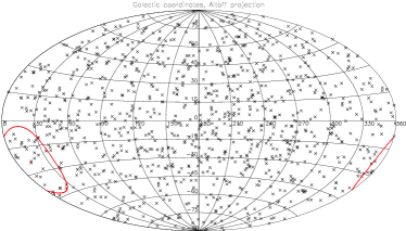
   Figure 1: The centres of 1000 patches randomly distributed on the sky used in this work (crosses). The red curve denotes the boundary of a random example patch of radius $r=20^{\circ}$ (red cross is its center).

2. Take the empirical distribution function $F_{\mathrm{p}}(x)$ of a given tested quantity $x$ of GRBs, e.g. $x=T_{90}$, $S$, $F$, etc. (see Section 2), for the whole sky. Number of GRBs in the data sample of the whole sky is $p=1591$.

3. Make 1 000 patches of a given radius $r$ randomly distributed on the sky. Afterwards we keep the positions of these patches fixed throughout our analysis (see Fig. 1).

4. For the GRBs in these 1 000 patches take the empirical distribution functions $G_{\mathrm{q}}(x)$ of the same property $x$. Number of GRBs in each patch is $q$ and it varies patch to patch.

5. For each patch compare the two empirical distribution functions $G_{\mathrm{q}}(x)$ and $F_{\mathrm{p}}(x)$ by calculating several test statistics $\xi=D$, $V$, $AD$, or $\chi^{2}$, where

   1. $D$ is the statistic of the two-sample Kolmogorov–Smirnov (K–S) test (Kolmogorov, 1933; Smirnov, 1939; Press et al., 2007) defined as

      $$D=\underset{-\infty<x<\infty}{\mathrm{max}}\left|F_{\mathrm{p}}(x)-G_{\mathrm{q}}(x)\right|$$ (1)

      Here $G_{\mathrm{q}}(x)$ and $F_{\mathrm{p}}(x)$ are the empirical cumulative distribution functions (see Fig. 2). The test statistic is the maximum value of the absolute difference between the two empirical cumulative distribution functions. Since the K–S test tends to be most sensitive around the median value of the distributions and less sensitive on the tails of the distributions we use also Kuiper’s $V$ and Anderson–Darling’s $AD$ statistics which provide increased sensitivity on the tails (Press et al. (2007)).

   2. $V$ is the statistic of the two-sample Kuiper test (Kuiper, 1960; Press et al., 2007) defined as

      $$\begin{split}V=D_{+}+D_{-}=\\ \underset{-\infty<x<\infty}{\mathrm{max}}\left[F_{\mathrm{p}}(x)-G_{\mathrm{q}}(x)\right]+\\ \underset{-\infty<x<\infty}{\mathrm{max}}\left[G_{\mathrm{q}}(x)-F_{\mathrm{p}}(x)\right]\end{split}$$ (2)

      Here $G_{\mathrm{q}}(x)$ and $F_{\mathrm{p}}(x)$ are the empirical cumulative distribution functions. The Kuiper’s test is related to the K–S test. The $D_{+}$ and $D_{-}$ represent the absolute values of the most positive and the most negative differences between the two empirical cumulative distribution functions.

   3. $AD$ is the statistic of the two-sample Anderson–Darling (A–D) test (Anderson & Darling, 1952; Darling, 1957; Pettitt, 1976) defined as

      $$\begin{split}AD\equiv A^{2}_{\mathrm{pq}}=\\ \frac{pq}{s}\int_{-\infty}^{\infty}\frac{[F_{p}(x)-G_{q}(x)]^{2}}{H_{s}(x)[1-H_{s}(x)]}dH_{s}(x),\end{split}$$ (3)

      where $G_{\mathrm{q}}(x)$, $F_{\mathrm{p}}(x)$ are the two empirical distribution functions being tested and the $H_{s}(x)=[pF_{p}(x)+qG_{q}(x)]/s$ with $s=p+q$ is the empirical distribution function of the pooled sample. The above integrand is defined to be zero whenever $H_{s}(x)=1$. For details see Scholz & Stephens (1987).

   4. $\chi^{2}$ is the statistic of the two-sample Chi-square test (Press et al., 2007). In case of $\chi^{2}$ the frequencies in the binned data of two samples are compared instead of the empirical distribution functions. The binning for both data sets, which are being compared, should be the same. We used $k=10$ number of bins and for this test we binned the logarithmic values: $\log x=\log T_{90}$, $\log S$, $\log F$, etc.. The $\chi^{2}$ is defined as

      $$\chi^{2}=\sum_{i=1}^{k}\frac{\left(K_{1}R_{i}-K_{2}Q_{i}\right)^{2}}{R_{i}+Q_{i}},$$ (4)

      where $k$ is the number of bins, $R_{i}$ is the observed frequency for bin $i$ for the first sample, and $Q_{i}$ is the observed frequency for bin $i$ for the second sample (see Fig. 3). $K_{1}$ and $K_{2}$ are the weights used to adjust for unequal sample sizes

      $$K_{1}=\sqrt{\frac{\sum_{i=1}^{k}Q_{i}}{\sum_{i=1}^{k}R_{i}}}$$ (5)

      and

      $$K_{2}=\sqrt{\frac{\sum_{i=1}^{k}R_{i}}{\sum_{i=1}^{k}Q_{i}}}.$$ (6)

6. This gives us a distribution of 1 000 values of $\xi^{\mathrm{m}}$ obtained from the measured data sample. In what follows the superscript $m$ used with any quantity, means that the quantity is related to the actual measured data sample.

7. In the next step we randomly shuffle our measured data sample. Each measurement is represented by a triplet $\{l_{\mathrm{i}}$, $b_{\mathrm{i}}$, $x_{\mathrm{i}}\}$. We randomly shuffle $x_{\mathrm{i}}$ keeping $l_{\mathrm{i}}$ and $b_{\mathrm{i}}$ fixed. In other words we keep the coordinates $l_{\mathrm{i}}$ and $b_{\mathrm{i}}$ of each measurement and we randomly shuffle the values $x_{\mathrm{i}}$ of each measurement. The actual values $x_{\mathrm{i}}$ remain unchanged, but they are randomly redistributed on the sky following the fixed measured positions $l_{\mathrm{i}}$ and $b_{\mathrm{i}}$.

8. For each patch on the sky we calculate the test statistic $\xi^{\mathrm{s}}$ again, but this time comparing the distributions of the shuffled data $G_{\mathrm{q}}^{\mathrm{s}}(x)$ for GRBs in each patch and the distribution for the whole sky $F_{\mathrm{p}}(x)$. In what follows the superscript $s$, used with any quantity, means that the quantity is related to randomly shuffled data.

9. We repeat the points 6. and 7. $n=100$ times. For some selected cases, when we want higher precision of our results, we repeat points 6. and 7. $n=1\,000$ times (see further in the text).

10. For a given statistic $\xi$ we derive the limiting values $\xi^{\mathrm{s}}_{10}$, $\xi^{\mathrm{s}}_{5}$, $\xi^{\mathrm{s}}_{1}$, and $\xi^{\mathrm{s}}_{0.1}$ which delimit the highest 10 %, 5 %, 1 %, and 0.1 % of all $\xi^{\mathrm{s}}$ values from all patches in all randomly shuffled data, respectively. In what follows we denote these limiting values as $\xi^{\mathrm{s}}_{\mathrm{i}}$, where i=10, 5, 1, or 0.1. $\xi^{\mathrm{s}}_{\mathrm{i}}$ is derived from a set of $10^{5}$ or $10^{6}$ values in case we have $n=100$ or $n=1\,000$ shufflings (see Fig. 4). For a given statistic $\xi$ we also derive value $\xi^{\mathrm{s}}_{0}$ which is the maximum of all $\xi^{\mathrm{s}}$ values in all patches of all shuffled data. The vales $\xi^{\mathrm{s}}_{0}$ are different for $n=100$ or $n=1\,000$ number of shufflings because they are derived from a set of $10^{5}$ or $10^{6}$ values, respectively.

11. We compare the distributions of a given statistic $\xi$ for the measured data and for all data shufflings. We count the number of patches $N^{\mathrm{m}}_{\mathrm{i}}$ in the measured data for which $\xi^{\mathrm{m}}>\xi^{\mathrm{s}}_{\mathrm{i}}$ (see Fig. 5).

12. The mean number of patches $\overline{N^{\mathrm{s}}_{\mathrm{i}}}$ in the randomly shuffled data for which $\xi^{\mathrm{s}}>\xi^{\mathrm{s}}_{\mathrm{i}}$ is $\overline{N^{\mathrm{s}}_{\mathrm{i}}}$ = 100, 50, 10, and 1 for i = 10, 5, 1, and 0.1, respectively. This means that, for example, if we find $N^{\mathrm{m}}_{\mathrm{1}}\gg 10$ it could indicate anisotropy in the measured data.

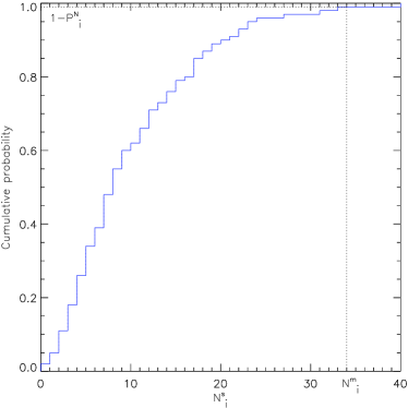
Figure 6: An example of the cumulative distribution of $N^{\mathrm{s}}_{\mathrm{i}}$, which is the number of patches with $\xi^{\mathrm{s}}>\xi^{\mathrm{s}}_{\mathrm{i}}$ in the randomly shuffled data. $N^{\mathrm{m}}_{\mathrm{i}}$ is the number of patches in the measured data for which $\xi^{\mathrm{m}}>\xi^{\mathrm{s}}_{\mathrm{i}}$. The probability (significance) $P^{\mathrm{N}}_{\mathrm{i}}$ of finding at least $N^{\mathrm{m}}_{\mathrm{i}}$ number of patches with $\xi^{\mathrm{s}}>\xi^{\mathrm{s}}_{\mathrm{i}}$ in the randomly shuffled data can be obtained from this distribution. This example result is for fluence $S$, $\xi=D$, $i=1$, patch radii $r=20^{\circ}$, and $n=100$ data shufflings. Here $N^{\mathrm{m}}_{\mathrm{i}}=N^{\mathrm{m}}_{\mathrm{1}}=34$ and $P^{\mathrm{N}}_{\mathrm{i}}=P^{\mathrm{N}}_{\mathrm{1}}=1\,\%$ (see Table 1).

13. In the last step we calculate the probability (significance) $P^{\mathrm{N}}_{\mathrm{i}}$ of finding at least $N^{\mathrm{m}}_{\mathrm{i}}$ number of patches with $\xi^{\mathrm{s}}>\xi^{\mathrm{s}}_{\mathrm{i}}$ in the randomly shuffled data (see Fig. 6).

14. Perform all steps for several radii of the patches $r=20^{\circ}$, $30^{\circ}$, $40^{\circ}$, $50^{\circ}$, $60^{\circ}$, for all tested quantities in our data sample $x=T_{90}$, $F_{64}$, $F_{256}$, $F_{1024}$, $F_{64\mathrm{,B}}$, $F_{256\mathrm{,B}}$, $F_{1024\mathrm{,B}}$, $S_{\mathrm{B}}$, $S$ and for all test statistics $\xi=AD$, $D$, $V$, and $\chi^{2}$.

Concerning our method one may object that the tested samples should be statistically independent, i.e. the sample of the whole sky should be independent of that being inside a patch. However, as mentioned in point 12., we derive the significances $P^{\mathrm{N}}_{\mathrm{i}}$ from the distribution of $N^{\mathrm{s}}_{\mathrm{i}}(\xi^{\mathrm{s}}>\xi^{\mathrm{s}}_{\mathrm{i}})$ in the randomly shuffled data, that means from a true distribution describing a randomized isotropic situation. We do not derive the significances $P^{\mathrm{N}}_{\mathrm{i}}$ from any theoretical distributions. Thus in our method the independence of the tested samples is not required.

We used routines “KSTWO” and “KUIPERTWO” of the IDL Astronomy Users Library (Landsman, 1993) for calculation of the $D$ and $V$ statistics, respectively. For the calculation of A–D statistic we employed the “adk” package (Scholz, 2012) of the R software (R Core Team, 2013).

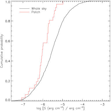
Figure 2: An example of two empirical cumulative distribution functions $F_{\mathrm{p}}(x)$ and $G_{\mathrm{q}}(x)$ of a GRB property $x$ obtained for all GRBs in the whole sky (black curve) and for all GRBs in one example sky patch (red curve), respectively. Both distributions are being compared by several test statistics. In this case $x$ is fluence $S$. This particular sky patch has radius of $r=20^{\circ}$ and center at the galactic coordinates of $l=28.6^{\circ}$ and $b=16.9^{\circ}$. It is the patch for which $D^{\mathrm{m}}_{\mathrm{0}}>D^{\mathrm{s}}_{\mathrm{0}}$ (see Table 1).

4 Results

This section describes the results obtained by the proposed method applied on the Fermi / GBM data sample. Fig. 2 shows an example of two empirical cumulative distribution functions of fluence $S$ obtained for the GRBs of the whole sky and for GRBs of one example sky patch. Both distributions are being compared by $AD$, $D$, and $V$ test statistics. Fig. 3 shows the same distributions, this time binned, which are being compared by $\chi^{2}$ statistic.

Fig. 4 shows an example of the distribution of the statistic $D$ obtained for all sky patches of radii $r=20^{\circ}$, all $n=100$ data shufflings, and fluences $S$. From such a distribution $D^{\mathrm{s}}_{10}$, $D^{\mathrm{s}}_{5}$, $D^{\mathrm{s}}_{1}$, $D^{\mathrm{s}}_{0.1}$, and $D^{\mathrm{s}}_{0}$ were calculated.

Fig. 5 shows an example of the comparison of the distributions of the statistic $D$ for the measured ($D^{\mathrm{m}}$) and shuffled ($D^{\mathrm{s}}$) data.

Fig. 6 shows an example of the cumulative distribution of $N^{\mathrm{s}}_{\mathrm{1}}$, which is the number of patches with $D^{\mathrm{s}}>D^{\mathrm{s}}_{\mathrm{1}}$ in the randomly shuffled data. This example result is for fluence $S$, patch radii $r=20^{\circ}$, and $n=100$ data shufflings. If we have $N^{\mathrm{m}}_{\mathrm{1}}$ the number of patches in the measured data for which $D^{\mathrm{m}}>D^{\mathrm{s}}_{\mathrm{1}}$, then from this figure one can obtain the chance probability (significance) $P^{\mathrm{N}}_{\mathrm{1}}$ of finding at least $N^{\mathrm{m}}_{\mathrm{1}}$ number of patches with $D^{\mathrm{s}}>D^{\mathrm{s}}_{\mathrm{1}}$ in the randomly shuffled data.

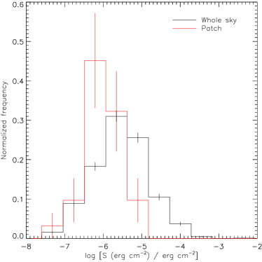
Figure 3: An example of two distributions of a GRB property $x$ obtained for the whole sky and for one example sky patch, which are being compared by $\chi^{2}$ statistic. In this case $x$ is fluence $S$. The black curve denotes the normalized frequencies $Q_{\mathrm{i}}/Q$ for the whole sky, where $Q_{\mathrm{i}}$ is the frequency in i-th bin and $Q$=1591 is the total number of events in the whole sky. The red curve denotes the normalized frequencies $R_{\mathrm{i}}/R$ for a sky patch, where $R_{\mathrm{i}}$ is the frequency in i-th bin and $R$=31 is the total number of events in the patch. This particular sky patch is the same as in Fig. 2 and it has radius of $r=20^{\circ}$ and center at the galactic coordinates of $l=28.6^{\circ}$ and $b=16.9^{\circ}$. The error bars over each bin are Poisson errors normalized by $Q$ or $R$, respectively.

Table 1 of Appendix A summarizes the results of all tested fluxes, fluences and duration of GRBs in the data sample using the Kolmogorov–Smirnov statistic $D$. The most important are columns $N^{\mathrm{m}}_{\mathrm{i}}$ and $P^{\mathrm{N}}_{\mathrm{i}}$. $N^{\mathrm{m}}_{\mathrm{i}}$ is the number of patches with $D^{\mathrm{m}}>D^{\mathrm{s}}_{\mathrm{i}}$ in the randomly shuffled data, where i=10, 5, 1, or 0.1. $P^{\mathrm{N}}_{\mathrm{i}}$ is the probability of finding at least $N^{\mathrm{m}}_{\mathrm{i}}$ number of patches with $D^{\mathrm{s}}>D^{\mathrm{s}}_{\mathrm{i}}$ in the randomly shuffled data. The randomly shuffled data are randomized samples and thus represent hypothetical isotropic samples. The cases with $P^{\mathrm{N}}_{\mathrm{i}}\leq 5$ %, are emphasized in boldface.

Concerning the fluences $S$, $S_{\mathrm{B}}$, peak fluxes $F_{64}$, $F_{256}$, $F_{1024}$, $F_{64\mathrm{,B}}$, $F_{256\mathrm{,B}}$ and patch radii $r=20^{\circ}$ or $r=30^{\circ}$ we obtained $P^{\mathrm{N}}_{\mathrm{5}}$, $P^{\mathrm{N}}_{\mathrm{1}}$, or $P^{\mathrm{N}}_{\mathrm{0.1}}$ $\leq 5$ %.

The most prominent discrepancy between the actual measured data and the randomly shuffled data is found for the peak flux $F_{64}$, patch radii $r=20^{\circ}$ and $n=1000$ data shufflings. The mean number of patches $\overline{N^{\mathrm{s}}_{\mathrm{0.1}}}$ in the randomly shuffled data for which $D^{\mathrm{s}}>D^{\mathrm{s}}_{\mathrm{0.1}}$ should be $\overline{N^{\mathrm{s}}_{\mathrm{0.1}}}=1$ because we applied 1000 sky patches. However, the actual measured data gives $N^{\mathrm{m}}_{\mathrm{0.1}}=14\gg 1$. The chance probability of finding at least 14 patches on the sky with $D^{\mathrm{s}}>D^{\mathrm{s}}_{\mathrm{0.1}}$ in the randomly shuffled data is only 0.4 %. This may indicate an anomaly in the measured data when compared to the simulated isotropic data samples.

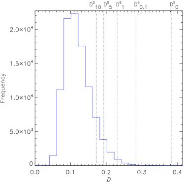
Figure 4: An example of the distribution of the statistic $D$ obtained for all sky patches and all $n=100$ data shufflings. Here the fluences $S$ and patch radii $r=20^{\circ}$ were used. The values $D^{\mathrm{s}}_{10}$, $D^{\mathrm{s}}_{5}$, $D^{\mathrm{s}}_{1}$, $D^{\mathrm{s}}_{0.1}$, and $D^{\mathrm{s}}_{0}$ are marked by vertical dotted lines.

Moreover, there are five cases concerning the fluences $S$, $S_{\mathrm{B}}$, peak fluxes $F_{64}$, $F_{256}$, and $F_{1024}$ (patch radii $r=20^{\circ}$ and 100 random data shufflings), where a patch gives the value of $D^{\mathrm{m}}$ in the measured data higher than the highest statistic $D^{\mathrm{s}}_{0}$ of all patches in all randomly shuffled data.

Table 2 of Appendix A summarizes the results of all tested GRB quantities in the data sample using the Kuiper statistic $V$. Again, the cases with $P^{\mathrm{N}}_{\mathrm{i}}\leq 5$ %, are emphasized in boldface.

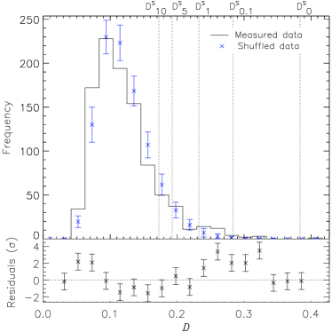
Figure 5: An example of the comparison of the distributions of the statistic $D$ for the measured ($D^{\mathrm{m}}$) and shuffled ($D^{\mathrm{s}}$) data. Here the fluences $S$ and patch radii $r=20^{\circ}$ were used. The blue crosses denote the mean frequencies for given bins and the error bars are corrected sample standard deviations $\sigma$ for $n=100$ data shufflings. The values $D^{\mathrm{s}}_{10}$, $D^{\mathrm{s}}_{5}$, $D^{\mathrm{s}}_{1}$, $D^{\mathrm{s}}_{0.1}$, and $D^{\mathrm{s}}_{0}$ marked by vertical dotted lines are the same as in Fig. 4. For example, here the number of patches in the measured data for which $D^{\mathrm{m}}>D^{\mathrm{s}}_{\mathrm{1}}$ is $N^{\mathrm{m}}_{\mathrm{1}}=34$ (see Table 1).

Concerning the fluence $S$, peak fluxes $F_{64}$, $F_{1024}$, $F_{64\mathrm{,B}}$ and patch radii $r=20^{\circ}$ or $r=40^{\circ}$ we obtained $P^{\mathrm{N}}_{\mathrm{10}}$, $P^{\mathrm{N}}_{\mathrm{5}}$, $P^{\mathrm{N}}_{\mathrm{1}}$, or $P^{\mathrm{N}}_{\mathrm{0.1}}$ $\leq 5$ %.

The most prominent discrepancy between the actual measured data and the randomly shuffled data is, similarly to the $D$ statistic, found for the peak flux $F_{64}$, patch radii $r=20^{\circ}$ and $n=1000$ data shufflings. The actual measured data gives $N^{\mathrm{m}}_{\mathrm{0.1}}=7\gg\overline{N^{\mathrm{s}}_{\mathrm{0.1}}}=1$. The chance probability of finding at least 7 patches on the sky with $V^{\mathrm{s}}>V^{\mathrm{s}}_{\mathrm{0.1}}$ in the randomly shuffled data is only 1.9 %.

Moreover, there are three cases concerning the fluence $S$, peak fluxes $F_{256}$, and $F_{1024}$ (patch radii $r=20^{\circ}$ and 100 random data shufflings), where a patch gives the value of $V^{\mathrm{m}}$ in the measured data higher than the highest statistic $V^{\mathrm{s}}_{0}$ of all patches in all randomly shuffled data.

Table 3 of Appendix A summarizes the results of all tested GRB quantities in the data sample using the Anderson–Darling statistic $AD$. The cases with $P^{\mathrm{N}}_{\mathrm{i}}\leq 5$ %, are emphasized in boldface.

Concerning the fluence $S$, peak fluxes $F_{64}$, $F_{64\mathrm{,B}}$, $F_{256\mathrm{,B}}$ and patch radii $r=20^{\circ}$ or $r=30^{\circ}$ we obtained $P^{\mathrm{N}}_{\mathrm{1}}$, or $P^{\mathrm{N}}_{\mathrm{0.1}}$ $\leq 5$ %.

The most prominent discrepancy between the actual measured data and the randomly shuffled data is found for the peak flux $F_{256\mathrm{,B}}$, patch radii $r=20^{\circ}$ and $n=100$ data shufflings. The actual measured data gives $N^{\mathrm{m}}_{\mathrm{0.1}}=10\gg\overline{N^{\mathrm{s}}_{\mathrm{0.1}}}=1$. The chance probability of finding at least 10 patches on the sky with $AD^{\mathrm{s}}>AD^{\mathrm{s}}_{\mathrm{0.1}}$ in the randomly shuffled data is only 1 %. This may indicate an anomaly in the measured data when compared to the simulated isotropic data samples.

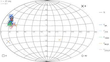
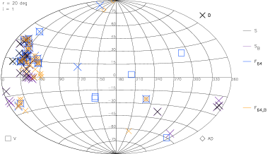
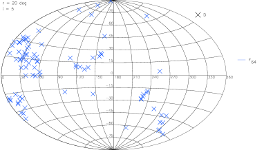
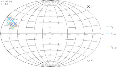
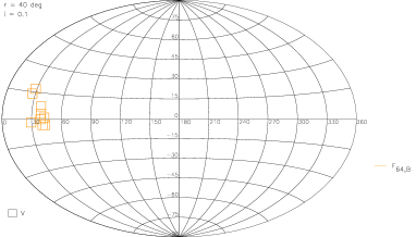
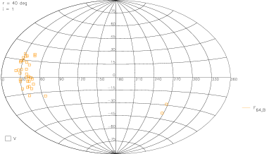
Figure 7: Plotted are the patch centers on the sky in Galactic Coordinates (Aitoff projection), for which the statistical properties of GRBs are mostly deviated from the randomness. The combined results for different statistics $\xi=D,V$, or $AD$: Kolmogorov–Smirnov’s $D$ (crosses), Kuiper’s $V$ (squares), or Anderson–Darling’s $AD$ (diamonds) are shown. Specifically, the markers (crosses, squares, or diamonds) denote the centers of the patches for which a given statistic $\xi^{\mathrm{m}}$, for the measured data, is higher than $\xi^{\mathrm{s}}_{\mathrm{i}}$ obtained from the randomly shuffled data and the significance $P^{\mathrm{N}}_{\mathrm{i}}\leq 5$ %, where i=5, 1, or 0.1. The size of the markers is inverse proportional to $P^{\mathrm{N}}_{\mathrm{i}}$. The exact values of $P^{\mathrm{N}}_{\mathrm{i}}$ can be found in Tables 1 – 4. Different colors mean different properties of GRBs being tested, particularly: fluences $S$ (black), $S_{\mathrm{B}}$ (violet), and peak fluxes $F_{64}$ (blue), $F_{256}$ (light blue), $F_{1024}$ (green), $F_{64\mathrm{,B}}$ (orange), $F_{256\mathrm{,B}}$ (red). In different pannels the results are plotted separately for different patch radii $r$ and for different $i$. The number of random data shufflings for these results is $n=1000$.

Moreover, there are two patches concerning the peak flux $F_{256\mathrm{,B}}$ (patch radius $r=20^{\circ}$ and 100 random data shufflings), which give the values of $AD^{\mathrm{m}}$ in the measured data higher than the highest statistic $AD^{\mathrm{s}}_{0}$ of all patches in all randomly shuffled data.

Table 4 of Appendix A summarizes the results of all tested GRB quantities in the data sample using the $\chi^{2}$ statistic. In the case of the $\chi^{2}$ statistic the probabilities $P^{\mathrm{N}}_{\mathrm{i}}$ were never lower or equal 5 %.

Also there is no case of a patch, of a given radius and for a given tested quantity in the measured data which gives $\chi^{\mathrm{2\,m}}$ higher than the highest $\chi^{\mathrm{2\,s}}_{0}$ for patches of all random data shufflings.

Unlike the previous three tests the two-sample Chi-square test is applied on the binned data of two samples instead of the unbinned empirical distribution functions. This may be the reason why this test is not as sensitive as the other three tests.

Fig. 7 shows the sky maps with marked patch centers for the cases where $P^{\mathrm{N}}_{\mathrm{i}}\leq 5$ % and for $\xi=D$, $V$, and $AD$ test statistics. It is interesting that for all three test statistics and various fluxes and fluences there is a prominent area on the sky with the center $l\approx 30^{\circ}$, $b\approx 15^{\circ}$ and radius $r\approx 20^{\circ}-40^{\circ}$, where the most patches with $\xi^{\mathrm{m}}>\xi^{\mathrm{s}}_{\mathrm{i}}$ are concentrated.

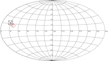
Figure 9: Plotted are the patch centers on the sky in Galactic Coordinates (Aitoff projection), which give the values of a given statistic $\xi^{\mathrm{m}}$ in the measured data higher than the highest statistic $\xi^{\mathrm{s}}_{0}$ of all patches in $n=100$ randomly shuffled data. The red diamonds mark the patch centers for Anderson–Darling’s $AD$ statistic and peak flux $F_{256\mathrm{,B}}$. The black cross marks one patch center for Kolmogorov–Smirnov’s $D$ statistic and for five tested quantities: fluxes $F_{64}$, $F_{256}$, $F_{1024}$ and fluences $S$, $S_{\mathrm{B}}$. The black square marks one patch center for Kuiper’s $V$ statistic and for three tested quantities: fluxes $F_{256}$, $F_{1024}$ and fluence $S$. All cases are for patch radii $r=20^{\circ}$.

Fig. 9 shows the patch centers on the sky which give the values of a given statistic $\xi^{\mathrm{m}}$ in the measured data higher than the highest statistic $\xi^{\mathrm{s}}_{0}$ of all patches in all $n=100$ randomly shuffled data. Since we have 1000 patches on the sky and $n=100$, it means that those patches in the measured data give the values of the statistic $\xi$ higher than any value obtained from the $10^{5}$ patches in the randomly shuffled sample.

In Fig. 4 and Fig. 8, we present the distributions of the peak fluxes $F_{64}$, $F_{256}$, $F_{1024}$, $F_{64\mathrm{,B}}$, $F_{256\mathrm{,B}}$ and fluences $S$, $S_{\mathrm{B}}$ obtained for the whole sky and for the sky patch of radius $r=20^{\circ}$ and its center at the galactic coordinates of $l=28.6^{\circ}$, $b=16.9^{\circ}$. For this particular direction and size of the patch we obtained the values of $D^{\mathrm{m}}$ and $V^{\mathrm{m}}$ in the measured data higher than the highest statistics $D^{\mathrm{s}}_{0}$ and $V^{\mathrm{s}}_{0}$, respectively, of all patches in all $n=100$ randomly shuffled data. It is the same direction as shown in Fig. 9.

5 Discussion

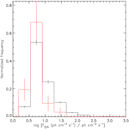
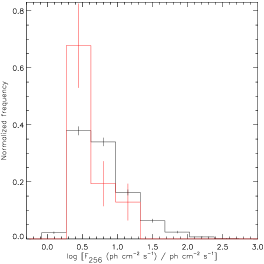
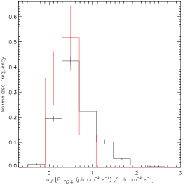
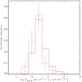
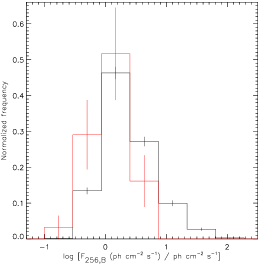
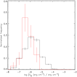
Figure 8: Figure shows the distributions of the peak fluxes $F_{64}$, $F_{256}$, $F_{1024}$, $F_{64\mathrm{,B}}$, $F_{256\mathrm{,B}}$ and fluence $S_{\mathrm{B}}$ obtained for the whole sky (black) and for one particular sky patch (red). The sky patch has radius of $r=20^{\circ}$ and center at the galactic coordinates of $l=28.6^{\circ}$, $b=16.9^{\circ}$. The center of this patch is marked by black cross and square in Fig. 9. The frequencies in each bin are normalized by the total number of events in the whole sky (1591) and in the patch (31), respectively. The error bars over each bin are Poisson errors, again normalized by the total number of events in the whole sky and in the patch, respectively.

In order to check if our results are not caused by an artefact due to the initial distribution of the patches on the sky, we again repeated our analysis starting with a different set of 1 000 randomly distributed patches on the sky and applied different $n=100$ random data shufflings. We again obtained practically the same results. There was a prominent area on the sky at the same position ($l\approx 30^{\circ}$, $b\approx 15^{\circ}$ and radius $r\approx 20^{\circ}-50^{\circ}$) with the excess (compared to the randomly shuffled data) of the patches with the highest values of the test statistics $D$, $V$, and $AD$. The probabilities $P^{\mathrm{N}}_{\mathrm{i}}\leq 5$ % were obtained for fluxes $F_{64}$, $F_{256}$, $F_{1024}$, $F_{64\mathrm{,B}}$, $F_{256\mathrm{,B}}$ and fluences $S_{\mathrm{B}}$, and $S$. The lowest chance probability was $P^{\mathrm{N}}_{\mathrm{i}}<1$ %.

Let us discuss the overall significance of finding an anisotropic signal using all the tests performed in this work. In our analysis we applied patches of five radii, nine different GRB properties and four statistics. For one limiting value, e.g. $\xi^{\mathrm{s}}_{0.1}$, this suggests 180 statistical tests, however many of these tests are not independent of each other. If we assume that there are 180 independent tests (trials) one can calculate the probability ($p-value$) of finding at least $k$ successes (each with probability $p$) from of the binomial test. For details see for example Eq. (1) and (2) of Vavrek et al. (2008). From Tables 1 – 4 one can see that we obtained: $k=14$ for $p\leq 5$ % then $p-value=8.8$ %; $k=9$ for $p\leq 3$ % then $p-value=12.1$ %; $k=4$ for $p\leq 2$ % then $p-value=78.6$ %. This is a course estimation because the tests are not independent. The number of independent tests (trials) is likely tens. We obtained that in one test the lowest chance probability obtained was 0.4 % (Kuiper’s $V$ statistic, peak flux $F_{64}$, energy range $(10-1000)$ keV and 64-ms timescale). However, for example, if the number of independent tests is 10 then for $p=0.4$ % the $p-value$ of the binomial test is 3.9 %. If the number of independent tests is 20 then the $p-value=7.7$ %. This suggests that a chance probability in a single test of 0.4 % is actually much more likely to occur by chance in one of the many tests used. Therefore likely our results do not point to a significant anisotropy.

It should be noted that the number of GRBs, in the patches centered at $l=28.6^{\circ}$ and $b=16.9^{\circ}$, are 31, 97, and 160 for the patch radii $r=20^{\circ},30^{\circ},40^{\circ}$, respectively. These numbers are lower than the mean values for all patches which are 48, 106, and 186 for the same patch radii, respectively. From the distributions of the numbers of GRBs contained in all patches of radii $r=20^{\circ},30^{\circ},40^{\circ}$ it follows that there are fractions of 99.0 %, 80.9 %, 97.5 %, respectively, of patches which contain the number of GRBs higher than the number of GRBs in the patches centered at $l=28.6^{\circ}$ and $b=16.9^{\circ}$ for the same patch sizes. It means that the GRBs found in the anomalous patch centered at $l=28.6^{\circ}$ and $b=16.9^{\circ}$ with radius $r=20^{\circ}$ do not only exhibit lower fluxes and fluence, as shown in Fig 3 and Fig 8, but also exhibit lower number density than what the mean value is. This is also demonstrated in Fig 10 where the centers of patches which represent the fraction of 5 % lowest occupied ones are plotted. The patch radii $20^{\circ}$, $30^{\circ}$, and $40^{\circ}$ are plotted separately. The area, where we found an anomaly, correlates with the less populated area on the sky. One can expect that the area of reduced GRB density will have relatively larger fluctuations in the measured GRB properties due to the Poisson noise. The Poisson noise in the areas of reduced GRB density not only effects the measured data, but also effects the randomly shuffled data. In our method we compare the number of patches which have values of a statistic higher than a given limit in the measured data with the number of patches having the same statistic higher than the same limit in the randomly shuffled data. Therefore this comparison of the measured data with the shuffled ones should make this method relatively robust. When we increased the number of the simulated randomly shuffled data samples from $n=100$ to $n=1000$ the statistical significance decreased.

Figure 10: Plotted are centers of the 5 % fraction of the lowest occupied patches for patch radii $20^{\circ}$, $30^{\circ}$, and $40^{\circ}$.

One may suggest that the anomalous direction found in the Fermi/GBM data could be due to some instrumental effects. Areas on the sky of decreased exposure and lower density of observed GRBs are expected for Fermi/GBM. The main reason is that some directions are less frequently observed due to occultation by the Earth. The direction towards the Earth is not entirely randomized on the sky because of the orbit and typical attitude of the Fermi satellite. Therefore one can expect regions of systematically deficient exposure time and thus deficient density of observed GRBs. Such effect was significant for Compton Gamma Ray Observatory (CGRO) (Fishman et al., 1993, 1994; Gehrels et al., 1993; Briggs et al., 1996; Hakkila et al., 2003), which had a similar low Earth orbit to Fermi. CGRO had inclination of $28.5^{\circ}$ and Fermi has inclination of $25.6^{\circ}$. Another question is if the Galactical gas and dust absorption can affect our results.

Horváth et al. (2014, 2015) studied the spatial distribution of GRBs, detected by Swift satellite (Gehrels et al., 2004), taking into account their redshift $z$. They used a two-dimensional Kolmogorov-Smirnov test, a nearest-neighbour test, and a bootstrap point-radius method applied on several sub-samples of different redshift intervals. They concluded that there was a statistically significant clustering of the GRB sample at $1.6<z\leq 2.1$ (Hercules–Corona Borealis Great Wall). From their Figure 3 of Horváth et al. (2014) or Figure 4 of Horváth et al. (2015) it is seen that the clustering happens at $l\approx 70^{\circ}$, $b\approx 45^{\circ}$ with a radius on the sky roughly about $r\approx 40^{\circ}$. It is interesting that the potential anomaly we found occurred in somewhat similar direction, however not exactly in the same one. Both areas are in the same quadrant on the sky and they partially overlap. This finding is also interesting considering that Horváth et al. (2014, 2015) used completely different approach and they studied number densities of GRBs on the sky for various redshift intervals employing a data set from a different satellite.

6 Conclusions

We tested the isotropy of the Universe through inspecting the isotropy of the properties of GRBs such as their duration, fluences and peak fluxes at various energy bands and different time scales. Summing up the results we conclude:

• We proposed a new method to test the isotropy of the Universe by testing the observed properties of GRBs from large datasets. The method was based on the comparisons of the distributions of a given measured GRB property for a large number of randomly spread patches on the sky with a distribution of the same GRB property for the whole sky. Four test statistics were applied to measure the differences between the distributions of the GRB properties for random sky patches and for the whole sky. The next key step was to compare the obtained distributions of the test statistics derived from the measured data with the distributions of the test statistics derived from randomly shuffled data to infer the significance of a potential anisotropy.

• We applied the method on the Fermi / GBM data sample with 1591 GRBs. We found that for three test statistics (Kolmogorov–Smirnov’s $D$, Kuiper’s $V$, Anderson–Darling’s $AD$) and various fluxes and fluences there is an area on the sky with the center $l\approx 30^{\circ}$, $b\approx 15^{\circ}$ and radius $r\approx 20^{\circ}-40^{\circ}$, where the most patches with the highest values of the test statistics are concentrated. The inferred chance probabilities of observing the obtained excess (compared to the randomly shuffled data) of the sky patches with high values of the test statistics went down below 5 % depending on the tested quantity and the test statistic used. However, many tests gave results consistent with isotropy.

• While we noticed a feature in the Fermi / GBM data, when we looked at the details more carefully we noticed a low number of GRBs in that particular patch and when we increased the number of the simulated randomly shuffled data samples the statistical significance decreased. Likely our results do not point to a significant anisotropy. Further investigation is highly desirable in order to confirm or reject these conclusions. A larger Fermi / GBM data sample as well as data samples of other GRB missions should be employed in the future and one should look for possible systematics.

Appendix A Tables with results

Table 1: Results using the Kolmogorov–Smirnov statistic $D$.

Tested	$r$	$n$	$D^{\mathrm{s}}_{10}$	$N^{\mathrm{m}}_{10}$	$P^{\mathrm{N}}_{10}$	$D^{\mathrm{s}}_{5}$	$N^{\mathrm{m}}_{5}$	$P^{\mathrm{N}}_{5}$	$D^{\mathrm{s}}_{1}$	$N^{\mathrm{m}}_{1}$	$P^{\mathrm{N}}_{1}$	$D^{\mathrm{s}}_{0.1}$	$N^{\mathrm{m}}_{0.1}$	$P^{\mathrm{N}}_{0.1}$	$D^{\mathrm{s}}_{0}$	$N^{\mathrm{m}}_{0}$	$D^{\mathrm{m}}_{0}$
quantity	(∘)				(%)			(%)			(%)			(%)
$T_{90}$	20	100	0.17	100	51	0.19	50	47	0.24	12	31	0.29	1	40	0.41	0	0.30
$T_{90}$	30	100	0.11	68	80	0.13	33	73	0.15	6	56	0.18	0	100	0.25	0	0.18
$T_{90}$	40	100	0.08	59	69	0.09	26	68	0.11	0	100	0.14	0	100	0.17	0	0.11
$T_{90}$	50	100	0.07	83	50	0.07	28	58	0.09	0	100	0.11	0	100	0.14	0	0.09
$T_{90}$	60	100	0.05	57	65	0.06	15	65	0.07	1	59	0.08	0	100	0.10	0	0.07
$S$	20	100	0.17	114	28	0.19	72	14	0.23	34	1	0.28	9	2	0.38	1	0.40
$S$	20	1000	0.17	113	30.2	0.19	72	13.1	0.23	30	2.2	0.28	9	1.1	0.42	0	0.40
$S$	30	100	0.11	89	58	0.13	60	29	0.15	23	13	0.19	3	9	0.24	0	0.20
$S$	40	100	0.08	95	49	0.09	50	40	0.11	4	57	0.13	0	100	0.15	0	0.12
$S$	50	100	0.07	66	71	0.07	24	73	0.09	4	49	0.10	0	100	0.12	0	0.09
$S$	60	100	0.05	52	64	0.06	18	62	0.07	1	53	0.09	0	100	0.11	0	0.07
$S_{\mathrm{B}}$	20	100	0.17	123	22	0.19	72	15	0.23	30	$<$1	0.28	5	6	0.36	1	0.36
$S_{\mathrm{B}}$	20	1000	0.17	124	17.3	0.19	74	11.5	0.23	31	1.4	0.29	3	12.8	0.47	0	0.36
$S_{\mathrm{B}}$	30	100	0.11	119	32	0.13	58	39	0.15	21	13	0.18	2	19	0.22	0	0.19
$S_{\mathrm{B}}$	40	100	0.08	79	56	0.09	46	44	0.11	1	80	0.14	0	100	0.19	0	0.12
$S_{\mathrm{B}}$	50	100	0.06	93	49	0.07	32	60	0.08	0	100	0.10	0	100	0.13	0	0.08
$S_{\mathrm{B}}$	60	100	0.05	97	37	0.06	36	48	0.07	2	55	0.08	0	100	0.10	0	0.07
$F_{64}$	20	100	0.17	145	8	0.19	87	4	0.23	34	2	0.28	15	$<$1	0.38	1	0.39
$F_{64}$	20	1000	0.17	144	5.6	0.19	87	3.4	0.23	30	1.5	0.28	14	0.4	0.42	0	0.39
$F_{64}$	30	100	0.11	124	27	0.13	74	19	0.15	33	3	0.18	13	1	0.24	0	0.22
$F_{64}$	30	1000	0.11	117	31.7	0.13	69	24.2	0.15	30	6.4	0.19	12	1.2	0.27	0	0.22
$F_{64}$	40	100	0.08	132	25	0.09	89	14	0.11	32	8	0.14	4	9	0.17	0	0.14
$F_{64}$	50	100	0.07	134	27	0.07	61	34	0.09	14	23	0.11	1	20	0.14	0	0.11
$F_{64}$	60	100	0.05	143	21	0.06	75	22	0.07	17	20	0.08	0	100	0.10	0	0.08
$F_{256}$	20	100	0.17	109	37	0.19	60	30	0.23	17	18	0.28	6	3	0.36	1	0.40
$F_{256}$	20	1000	0.17	107	38.9	0.19	58	31.7	0.23	17	18.3	0.29	6	3.5	0.41	0	0.40
$F_{256}$	30	100	0.11	108	36	0.13	69	23	0.15	26	12	0.18	8	2	0.23	0	0.23
$F_{256}$	30	1000	0.11	103	43.8	0.13	65	26.8	0.15	25	9.6	0.18	8	3.6	0.25	0	0.23
$F_{256}$	40	100	0.08	140	23	0.09	87	17	0.11	31	10	0.14	2	11	0.20	0	0.15
$F_{256}$	50	100	0.07	143	23	0.07	76	25	0.09	27	12	0.11	6	7	0.14	0	0.12
$F_{256}$	60	100	0.05	166	25	0.06	93	22	0.07	35	11	0.08	2	11	0.10	0	0.09
$F_{1024}$	20	100	0.17	78	76	0.19	43	63	0.23	13	28	0.28	6	2	0.36	1	0.37
$F_{1024}$	20	1000	0.17	74	84.8	0.19	40	69.9	0.23	13	29.6	0.28	6	2.9	0.44	0	0.37
$F_{1024}$	30	100	0.11	68	77	0.13	33	70	0.15	11	31	0.18	1	26	0.23	0	0.20
$F_{1024}$	40	100	0.08	51	81	0.09	27	66	0.11	2	65	0.14	0	100	0.18	0	0.12
$F_{1024}$	50	100	0.07	83	48	0.07	35	48	0.09	7	31	0.10	0	100	0.13	0	0.10
$F_{1024}$	60	100	0.05	78	49	0.06	41	43	0.07	6	43	0.08	0	100	0.09	0	0.07
$F_{64\mathrm{,B}}$	20	100	0.17	131	13	0.19	78	4	0.23	28	2	0.28	7	3	0.41	0	0.32
$F_{64\mathrm{,B}}$	20	1000	0.17	129	15.7	0.19	78	8.9	0.23	28	2.7	0.28	6	3.4	0.42	0	0.32
$F_{64\mathrm{,B}}$	30	100	0.11	123	26	0.13	74	20	0.15	25	11	0.19	3	9	0.24	0	0.20
$F_{64\mathrm{,B}}$	30	1000	0.11	125	26.2	0.13	75	18.2	0.15	25	9.1	0.18	5	6.6	0.26	0	0.20
$F_{64\mathrm{,B}}$	40	100	0.08	131	29	0.09	82	18	0.11	21	16	0.13	3	14	0.17	0	0.15
$F_{64\mathrm{,B}}$	40	1000	0.08	130	26.2	0.09	78	19.8	0.11	21	15.8	0.13	3	10.0	0.21	0	0.15
$F_{64\mathrm{,B}}$	50	100	0.07	107	40	0.08	48	46	0.09	0	100	0.11	0	100	0.17	0	0.09
$F_{64\mathrm{,B}}$	60	100	0.05	109	38	0.06	41	47	0.07	5	41	0.08	0	100	0.10	0	0.07
$F_{256\mathrm{,B}}$	20	100	0.17	103	48	0.19	60	34	0.23	26	5	0.28	5	3	0.37	0	0.32
$F_{256\mathrm{,B}}$	20	1000	0.17	99	49.7	0.19	60	27.2	0.23	23	6.4	0.28	5	5.8	0.41	0	0.32
$F_{256\mathrm{,B}}$	30	100	0.11	99	53	0.13	66	27	0.15	13	29	0.19	0	100	0.23	0	0.19
$F_{256\mathrm{,B}}$	40	100	0.08	74	62	0.09	45	44	0.11	7	39	0.14	0	100	0.19	0	0.14
$F_{256\mathrm{,B}}$	50	100	0.07	71	63	0.07	24	63	0.09	2	55	0.11	0	100	0.13	0	0.09
$F_{256\mathrm{,B}}$	60	100	0.05	82	46	0.06	42	39	0.07	4	34	0.09	0	100	0.11	0	0.07
$F_{1024\mathrm{,B}}$	20	100	0.17	90	66	0.19	58	34	0.23	8	58	0.29	1	39	0.37	0	0.31
$F_{1024\mathrm{,B}}$	30	100	0.11	98	50	0.13	53	37	0.15	8	43	0.18	0	100	0.25	0	0.17
$F_{1024\mathrm{,B}}$	40	100	0.09	84	48	0.09	40	47	0.12	1	73	0.14	0	100	0.17	0	0.12
$F_{1024\mathrm{,B}}$	50	100	0.07	111	35	0.07	52	35	0.09	6	33	0.11	0	100	0.14	0	0.09
$F_{1024\mathrm{,B}}$	60	100	0.05	147	25	0.06	63	31	0.07	8	36	0.08	0	100	0.10	0	0.07

Table 2: Results using the Kuiper statistic $V$.

Tested	$r$	$n$	$V^{\mathrm{s}}_{10}$	$N^{\mathrm{m}}_{10}$	$P^{\mathrm{N}}_{10}$	$V^{\mathrm{s}}_{5}$	$N^{\mathrm{m}}_{5}$	$P^{\mathrm{N}}_{5}$	$V^{\mathrm{s}}_{1}$	$N^{\mathrm{m}}_{1}$	$P^{\mathrm{N}}_{1}$	$V^{\mathrm{s}}_{0.1}$	$N^{\mathrm{m}}_{0.1}$	$P^{\mathrm{N}}_{0.1}$	$V^{\mathrm{s}}_{0}$	$N^{\mathrm{m}}_{0}$	$V^{\mathrm{m}}_{0}$
quantity	(∘)				(%)			(%)			(%)			(%)
$T_{90}$	20	100	0.23	120	23	0.25	57	32	0.29	14	25	0.34	0	100	0.41	0	0.33
$T_{90}$	30	100	0.15	138	14	0.16	82	9	0.19	12	32	0.22	0	100	0.27	0	0.21
$T_{90}$	40	100	0.11	112	36	0.12	41	57	0.14	7	44	0.16	0	100	0.19	0	0.15
$T_{90}$	50	100	0.09	109	36	0.09	37	55	0.11	3	58	0.12	0	100	0.14	0	0.11
$T_{90}$	60	100	0.07	115	36	0.08	46	43	0.09	5	46	0.10	0	100	0.12	0	0.09
$S$	20	100	0.23	96	59	0.25	63	22	0.28	23	9	0.34	6	5	0.40	1	0.41
$S$	20	1000	0.23	95	55.5	0.25	62	23.7	0.29	23	5.6	0.33	6	3.3	0.51	0	0.41
$S$	30	100	0.15	87	66	0.16	50	49	0.19	15	21	0.22	0	100	0.27	0	0.22
$S$	40	100	0.11	61	71	0.12	29	68	0.14	6	48	0.16	0	100	0.21	0	0.15
$S$	50	100	0.09	24	91	0.09	5	93	0.11	0	100	0.12	0	100	0.14	0	0.10
$S$	60	100	0.07	15	95	0.08	2	98	0.09	0	100	0.10	0	100	0.12	0	0.08
$S_{\mathrm{B}}$	20	100	0.23	110	33	0.25	68	15	0.29	23	6	0.34	3	14	0.42	0	0.37
$S_{\mathrm{B}}$	20	1000	0.23	108	35.6	0.25	66	18.0	0.29	23	5.9	0.34	3	13.2	0.49	0	0.37
$S_{\mathrm{B}}$	30	100	0.15	101	52	0.16	54	43	0.19	20	12	0.22	1	40	0.28	0	0.22
$S_{\mathrm{B}}$	40	100	0.11	57	70	0.12	29	62	0.14	3	58	0.16	0	100	0.19	0	0.15
$S_{\mathrm{B}}$	50	100	0.08	42	87	0.09	10	95	0.10	0	100	0.12	0	100	0.15	0	0.10
$S_{\mathrm{B}}$	60	100	0.07	22	91	0.07	5	92	0.08	0	100	0.10	0	100	0.11	0	0.08
$F_{64}$	20	100	0.23	141	5	0.25	77	9	0.28	27	2	0.33	7	2	0.42	0	0.40
$F_{64}$	20	1000	0.23	140	6.3	0.25	77	6.6	0.29	27	2.4	0.33	7	1.9	0.45	0	0.40
$F_{64}$	30	100	0.15	112	38	0.16	66	28	0.19	24	11	0.21	5	7	0.26	0	0.22
$F_{64}$	30	1000	0.15	112	35.5	0.16	68	24.6	0.19	24	9.9	0.22	4	8.2	0.28	0	0.22
$F_{64}$	40	100	0.11	116	28	0.12	64	25	0.14	22	17	0.16	3	14	0.18	0	0.16
$F_{64}$	50	100	0.09	121	33	0.09	51	38	0.11	4	48	0.12	0	100	0.16	0	0.11
$F_{64}$	60	100	0.07	119	28	0.08	50	38	0.09	1	66	0.10	0	100	0.13	0	0.09
$F_{256}$	20	100	0.23	110	29	0.25	53	40	0.29	14	28	0.33	4	10	0.41	1	0.43
$F_{256}$	20	1000	0.23	110	34.7	0.25	52	42.6	0.29	14	25.4	0.34	4	8.5	0.48	0	0.43
$F_{256}$	30	100	0.15	107	36	0.16	62	29	0.19	18	19	0.22	1	29	0.26	0	0.25
$F_{256}$	30	1000	0.15	106	40.5	0.16	61	30.1	0.19	18	17.5	0.22	1	32.4	0.26	0	0.25
$F_{256}$	40	100	0.11	135	23	0.12	75	24	0.14	20	15	0.16	2	10	0.21	0	0.17
$F_{256}$	50	100	0.09	128	28	0.09	67	30	0.11	15	21	0.13	1	18	0.15	0	0.13
$F_{256}$	60	100	0.07	132	27	0.07	70	25	0.08	19	18	0.10	0	100	0.12	0	0.10
$F_{1024}$	20	100	0.23	76	78	0.25	48	56	0.28	13	30	0.33	6	4	0.41	1	0.42
$F_{1024}$	20	1000	0.23	76	82.0	0.25	48	52.6	0.29	13	30.5	0.34	5	4.7	0.50	0	0.42
$F_{1024}$	30	100	0.15	53	88	0.16	36	65	0.19	8	44	0.22	1	30	0.25	0	0.24
$F_{1024}$	40	100	0.11	35	92	0.12	12	92	0.14	0	100	0.16	0	100	0.19	0	0.14
$F_{1024}$	50	100	0.09	47	86	0.09	17	85	0.11	1	83	0.12	0	100	0.14	0	0.11
$F_{1024}$	60	100	0.07	27	85	0.07	5	92	0.08	0	100	0.10	0	100	0.11	0	0.08
$F_{64\mathrm{,B}}$	20	100	0.23	141	10	0.25	72	14	0.29	23	8	0.34	3	12	0.50	0	0.34
$F_{64\mathrm{,B}}$	20	1000	0.23	137	9.2	0.25	67	17.2	0.29	23	5.8	0.33	3	13.7	0.48	0	0.34
$F_{64\mathrm{,B}}$	30	100	0.15	137	16	0.16	84	12	0.19	24	10	0.22	1	34	0.31	0	0.22
$F_{64\mathrm{,B}}$	30	1000	0.15	137	17.7	0.16	81	13.7	0.19	24	9.7	0.22	1	31.5	0.28	0	0.22
$F_{64\mathrm{,B}}$	40	100	0.11	119	37	0.12	78	22	0.14	35	9	0.16	9	4	0.19	0	0.18
$F_{64\mathrm{,B}}$	40	1000	0.11	121	31.1	0.12	78	17.8	0.14	35	4.7	0.16	9	2.5	0.23	0	0.18
$F_{64\mathrm{,B}}$	50	100	0.09	91	46	0.10	54	34	0.11	11	28	0.13	0	100	0.17	0	0.13
$F_{64\mathrm{,B}}$	60	100	0.07	52	77	0.08	26	71	0.09	9	38	0.10	0	100	0.12	0	0.10
$F_{256\mathrm{,B}}$	20	100	0.23	105	41	0.25	68	19	0.28	22	10	0.33	1	43	0.44	0	0.34
$F_{256\mathrm{,B}}$	20	1000	0.23	103	43.0	0.25	64	20.9	0.29	21	7.3	0.33	1	43.9	0.46	0	0.34
$F_{256\mathrm{,B}}$	30	100	0.15	74	71	0.16	40	62	0.19	13	27	0.21	0	100	0.27	0	0.21
$F_{256\mathrm{,B}}$	40	100	0.11	66	72	0.12	43	50	0.14	9	36	0.16	0	100	0.24	0	0.15
$F_{256\mathrm{,B}}$	50	100	0.09	54	76	0.09	18	79	0.11	2	65	0.12	0	100	0.16	0	0.11
$F_{256\mathrm{,B}}$	60	100	0.07	58	63	0.07	30	59	0.09	7	36	0.10	0	100	0.12	0	0.09
$F_{1024\mathrm{,B}}$	20	100	0.23	98	49	0.25	52	43	0.29	15	19	0.33	0	100	0.46	0	0.32
$F_{1024\mathrm{,B}}$	30	100	0.15	102	40	0.16	59	33	0.19	8	49	0.22	0	100	0.28	0	0.22
$F_{1024\mathrm{,B}}$	40	100	0.11	111	37	0.12	47	44	0.14	2	75	0.16	0	100	0.20	0	0.15
$F_{1024\mathrm{,B}}$	50	100	0.09	138	26	0.09	58	33	0.11	7	42	0.12	0	100	0.15	0	0.11
$F_{1024\mathrm{,B}}$	60	100	0.07	122	33	0.07	58	32	0.09	1	67	0.10	0	100	0.11	0	0.09

Table 3: Results using the Anderson–Darling statistic $AD$.

Tested	$r$	$n$	$AD^{\mathrm{s}}_{10}$	$N^{\mathrm{m}}_{10}$	$P^{\mathrm{N}}_{10}$	$AD^{\mathrm{s}}_{5}$	$N^{\mathrm{m}}_{5}$	$P^{\mathrm{N}}_{5}$	$AD^{\mathrm{s}}_{1}$	$N^{\mathrm{m}}_{1}$	$P^{\mathrm{N}}_{1}$	$AD^{\mathrm{s}}_{0.1}$	$N^{\mathrm{m}}_{0.1}$	$P^{\mathrm{N}}_{0.1}$	$AD^{\mathrm{s}}_{0}$	$N^{\mathrm{m}}_{0}$	$AD^{\mathrm{m}}_{0}$
quantity	(∘)				(%)			(%)			(%)			(%)
$T_{90}$	20	100	1.80	99	50	2.32	32	79	3.61	5	71	5.82	0	100	14.00	0	4.41
$T_{90}$	30	100	1.65	70	75	2.12	31	70	3.28	1	92	5.35	0	100	9.96	0	3.31
$T_{90}$	40	100	1.57	57	73	2.04	21	70	3.16	1	68	4.92	0	100	7.94	0	3.18
$T_{90}$	50	100	1.33	68	62	1.72	23	60	2.72	1	56	4.31	0	100	6.89	0	2.97
$T_{90}$	60	100	1.20	49	67	1.54	19	65	2.27	0	100	3.32	0	100	4.89	0	2.19
$S$	20	100	1.81	117	29	2.33	74	12	3.61	24	3	5.45	1	36	10.33	0	7.74
$S$	20	1000	1.81	117	28.5	2.33	74	12.7	3.62	24	7.0	5.56	1	35.7	14.90	0	7.74
$S$	30	100	1.71	90	51	2.22	56	35	3.45	15	24	5.34	0	100	8.93	0	4.70
$S$	40	100	1.50	80	57	1.94	25	71	3.00	2	70	4.45	0	100	6.95	0	3.62
$S$	50	100	1.37	70	64	1.75	26	69	2.63	3	57	4.09	0	100	6.25	0	2.81
$S$	60	100	1.24	86	48	1.62	20	57	2.52	0	100	3.68	0	100	6.07	0	2.39
$S_{\mathrm{B}}$	20	100	1.86	113	34	2.40	53	44	3.71	16	20	5.57	1	35	9.58	0	6.99
$S_{\mathrm{B}}$	20	1000	1.81	117	27.2	2.34	62	26.0	3.61	18	14.8	5.53	1	37.3	11.47	0	6.99
$S_{\mathrm{B}}$	30	100	1.65	90	50	2.11	54	36	3.30	11	31	5.11	0	100	7.93	0	4.38
$S_{\mathrm{B}}$	40	100	1.58	39	84	2.04	13	88	3.18	0	100	5.07	0	100	10.90	0	2.80
$S_{\mathrm{B}}$	50	100	1.31	50	81	1.68	13	84	2.52	0	100	3.93	0	100	8.75	0	2.10
$S_{\mathrm{B}}$	60	100	1.07	75	52	1.38	24	58	2.10	0	100	3.17	0	100	4.78	0	1.91
$F_{64}$	20	100	1.80	129	22	2.32	66	24	3.62	19	15	5.68	2	18	9.06	0	6.77
$F_{64}$	20	1000	1.82	125	19.6	2.35	65	22.2	3.63	19	14.4	5.56	3	12.2	14.19	0	6.77
$F_{64}$	30	100	1.65	111	36	2.12	68	22	3.29	20	12	5.11	5	4	7.97	0	5.67
$F_{64}$	30	1000	1.69	106	41.0	2.18	60	32.7	3.41	19	18.3	5.19	5	8.3	12.32	0	5.67
$F_{64}$	40	100	1.56	114	35	2.02	57	30	3.12	11	24	4.74	0	100	8.25	0	3.82
$F_{64}$	50	100	1.40	101	44	1.80	50	40	2.88	23	15	4.43	1	18	6.00	0	4.70
$F_{64}$	60	100	1.20	112	37	1.55	77	18	2.38	29	8	3.50	3	7	5.37	0	3.70
$F_{256}$	20	100	1.81	102	46	2.31	48	47	3.55	12	34	5.35	2	21	8.65	0	6.62
$F_{256}$	20	1000	1.83	100	48.5	2.36	46	53.8	3.67	11	38.2	5.65	1	34.0	12.24	0	6.62
$F_{256}$	30	100	1.67	97	49	2.15	55	37	3.31	13	25	4.93	1	30	10.28	0	5.35
$F_{256}$	30	1000	1.69	93	51.2	2.18	52	40.9	3.36	12	32.6	5.07	1	27.6	10.24	0	5.35
$F_{256}$	40	100	1.49	103	45	1.91	50	44	3.05	4	49	5.05	0	100	8.61	0	3.44
$F_{256}$	50	100	1.37	109	41	1.78	48	41	2.83	14	25	4.14	1	21	6.76	0	4.31
$F_{256}$	60	100	1.13	140	30	1.49	63	32	2.36	29	16	3.61	0	100	6.13	0	3.50
$F_{1024}$	20	100	1.78	74	80	2.28	43	62	3.51	7	63	5.23	1	39	10.10	0	6.10
$F_{1024}$	20	1000	1.81	71	83.9	2.33	41	64.9	3.61	7	61.7	5.58	1	34.8	11.48	0	6.10
$F_{1024}$	30	100	1.69	64	81	2.17	42	59	3.40	4	61	5.36	0	100	9.26	0	4.31
$F_{1024}$	40	100	1.56	47	78	2.02	9	92	3.14	0	100	4.82	0	100	8.13	0	2.62
$F_{1024}$	50	100	1.38	82	51	1.78	49	35	2.80	8	27	4.21	0	100	6.97	0	3.88
$F_{1024}$	60	100	1.15	113	38	1.47	76	23	2.27	22	16	3.44	0	100	5.05	0	2.86
$F_{64\mathrm{,B}}$	20	100	1.80	121	22	2.33	71	13	3.65	29	3	5.67	5	6	10.11	0	7.51
$F_{64\mathrm{,B}}$	20	1000	1.81	119	26.0	2.33	71	17.0	3.60	29	3.4	5.54	7	2.9	12.96	0	7.51
$F_{64\mathrm{,B}}$	30	100	1.71	121	30	2.20	81	16	3.39	32	5	5.32	7	4	8.56	0	6.69
$F_{64\mathrm{,B}}$	30	1000	1.69	122	29.1	2.18	81	14.9	3.39	31	6.4	5.22	10	2.2	10.29	0	6.69
$F_{64\mathrm{,B}}$	40	100	1.49	161	18	1.92	107	12	2.97	27	10	4.57	1	23	6.89	0	5.30
$F_{64\mathrm{,B}}$	40	1000	1.52	157	14.8	1.95	104	10.0	3.03	26	12.9	4.75	1	19.9	10.57	0	5.30
$F_{64\mathrm{,B}}$	50	100	1.42	139	25	1.85	72	29	2.96	8	36	4.78	0	100	7.38	0	4.65
$F_{64\mathrm{,B}}$	60	100	1.16	144	26	1.51	68	27	2.33	11	28	3.50	0	100	5.80	0	2.83
$F_{256\mathrm{,B}}$	20	100	1.80	99	47	2.29	62	26	3.43	30	1	5.09	10	1	7.69	2	8.98
$F_{256\mathrm{,B}}$	20	1000	1.81	98	50.7	2.34	58	31.6	3.65	25	5.7	5.57	8	2.6	11.01	0	8.98
$F_{256\mathrm{,B}}$	30	100	1.71	107	42	2.22	66	28	3.56	27	10	5.64	3	11	9.56	0	6.55
$F_{256\mathrm{,B}}$	40	100	1.56	106	40	2.02	73	26	3.21	9	28	5.39	0	100	8.73	0	4.34
$F_{256\mathrm{,B}}$	50	100	1.39	107	38	1.81	42	45	2.82	4	45	4.66	0	100	9.79	0	3.45
$F_{256\mathrm{,B}}$	60	100	1.11	122	29	1.43	49	36	2.24	0	100	3.79	0	100	7.34	0	2.07
$F_{1024\mathrm{,B}}$	20	100	1.80	103	45	2.32	53	41	3.64	15	18	5.70	4	8	9.36	0	6.69
$F_{1024\mathrm{,B}}$	30	100	1.67	83	62	2.14	46	50	3.24	24	11	4.89	2	18	8.21	0	5.64
$F_{1024\mathrm{,B}}$	40	100	1.58	99	43	2.03	41	45	3.24	3	48	4.92	0	100	8.52	0	3.60
$F_{1024\mathrm{,B}}$	50	100	1.37	109	38	1.77	55	36	2.74	4	39	4.21	0	100	6.50	0	3.18
$F_{1024\mathrm{,B}}$	60	100	1.14	135	26	1.46	54	33	2.22	0	100	3.30	0	100	4.78	0	2.22

Table 4: Results using the $\chi^{2}$ statistic.

Tested	$r$	$n$	$\chi_{10}^{\mathrm{2\,s}}$	$N^{\mathrm{m}}_{10}$	$P^{\mathrm{N}}_{10}$	$\chi_{5}^{\mathrm{2\,s}}$	$N^{\mathrm{m}}_{5}$	$P^{\mathrm{N}}_{5}$	$\chi_{1}^{\mathrm{2\,s}}$	$N^{\mathrm{m}}_{1}$	$P^{\mathrm{N}}_{1}$	$\chi_{0.1}^{\mathrm{2\,s}}$	$N^{\mathrm{m}}_{0.1}$	$P^{\mathrm{N}}_{0.1}$	$\chi_{0}^{\mathrm{2\,s}}$	$N^{\mathrm{m}}_{0}$	$\chi_{0}^{\mathrm{2\,m}}$
quantity	(∘)				(%)			(%)			(%)			(%)
$T_{90}$	20	100	14.36	73	94	18.19	34	87	26.52	0	100	38.71	0	100	72.21	0	25.23
$T_{90}$	30	100	12.41	65	82	14.45	26	82	18.96	0	100	25.98	0	100	46.44	0	17.91
$T_{90}$	40	100	10.84	34	94	12.53	9	94	16.10	0	100	20.73	0	100	31.63	0	13.88
$T_{90}$	50	100	9.67	12	96	11.11	1	98	14.13	0	100	17.79	0	100	26.37	0	11.22
$T_{90}$	60	100	8.20	22	95	9.33	10	88	11.60	0	100	14.70	0	100	19.08	0	10.50
$S$	20	100	12.33	86	78	16.47	49	51	23.59	4	82	31.53	0	100	47.54	0	26.45
$S$	20	1000	12.36	86	69.9	16.40	49	48.6	24.16	4	78.2	32.75	0	100.0	57.12	0	26.45
$S$	30	100	11.47	75	75	13.49	40	60	17.82	1	90	23.69	0	100	37.34	0	17.93
$S$	40	100	10.07	38	92	11.65	17	86	15.01	3	67	20.04	0	100	28.36	0	18.41
$S$	50	100	8.84	49	81	10.15	11	86	12.95	0	100	17.14	0	100	23.64	0	12.31
$S$	60	100	7.81	36	78	8.98	16	70	11.56	0	100	15.45	0	100	22.07	0	11.24
$S_{\mathrm{B}}$	20	100	12.14	99	51	15.84	56	32	24.21	7	57	32.18	0	100	46.75	0	27.66
$S_{\mathrm{B}}$	20	1000	12.29	98	52.4	16.09	54	34.3	24.21	7	59.6	32.46	0	100.0	54.78	0	27.66
$S_{\mathrm{B}}$	30	100	11.31	78	77	13.25	49	49	17.62	12	40	22.97	0	100	31.47	0	22.91
$S_{\mathrm{B}}$	40	100	10.21	64	71	11.87	29	68	15.38	5	52	22.19	0	100	30.88	0	16.85
$S_{\mathrm{B}}$	50	100	8.76	47	82	10.09	19	81	12.66	0	100	15.76	0	100	21.94	0	12.51
$S_{\mathrm{B}}$	60	100	7.56	37	83	8.72	4	90	11.15	0	100	14.29	0	100	18.90	0	9.15
$F_{64}$	20	100	13.74	100	50	18.36	49	51	25.56	4	72	35.47	0	100	47.58	0	31.03
$F_{64}$	20	1000	14.12	97	55.9	18.60	43	69.5	25.93	3	78.3	37.04	0	100.0	67.73	0	31.03
$F_{64}$	30	100	11.17	48	98	13.36	1	100	17.92	0	100	23.27	0	100	37.76	0	15.18
$F_{64}$	30	1000	11.25	47	96.7	13.46	1	100.0	18.19	0	100.0	24.32	0	100.0	43.52	0	15.18
$F_{64}$	40	100	9.63	16	98	11.30	0	100	14.79	0	100	19.27	0	100	25.77	0	10.79
$F_{64}$	50	100	8.16	33	91	9.47	3	98	12.05	0	100	15.49	0	100	20.89	0	10.06
$F_{64}$	60	100	7.22	46	72	8.29	18	69	10.61	0	100	13.93	0	100	18.45	0	9.42
$F_{256}$	20	100	15.18	102	48	19.75	36	84	27.21	3	86	39.02	0	100	52.37	0	32.76
$F_{256}$	20	1000	15.18	102	44.0	19.59	38	80.8	27.34	3	80.1	39.09	0	100.0	70.76	0	32.76
$F_{256}$	30	100	12.29	89	63	14.50	21	86	18.75	0	100	24.56	0	100	40.75	0	18.50
$F_{256}$	30	1000	12.31	87	64.6	14.55	19	91.2	19.33	0	100.0	26.07	0	100.0	43.41	0	18.50
$F_{256}$	40	100	10.48	115	37	12.20	55	38	15.89	3	58	21.13	0	100	32.99	0	17.45
$F_{256}$	50	100	9.17	149	22	10.57	75	22	13.43	2	65	17.08	0	100	27.19	0	14.26
$F_{256}$	60	100	7.79	130	32	8.87	72	33	11.08	9	36	13.87	0	100	18.15	0	13.07
$F_{1024}$	20	100	12.32	69	93	16.53	47	55	24.45	5	72	33.62	0	100	49.01	0	26.11
$F_{1024}$	20	1000	12.47	69	93.8	16.65	47	57.5	24.97	4	76.2	34.41	0	100.0	72.58	0	26.11
$F_{1024}$	30	100	11.40	36	100	13.54	8	99	18.11	0	100	25.29	0	100	35.62	0	17.67
$F_{1024}$	40	100	9.97	8	100	11.57	0	100	14.97	0	100	18.96	0	100	24.45	0	11.13
$F_{1024}$	50	100	8.68	12	98	10.01	2	96	12.87	0	100	17.03	0	100	23.33	0	10.20
$F_{1024}$	60	100	7.45	18	93	8.63	4	93	11.00	0	100	14.31	0	100	21.06	0	10.57
$F_{64\mathrm{,B}}$	20	100	15.89	107	35	20.10	59	24	28.89	16	23	44.08	1	23	64.67	0	44.28
$F_{64\mathrm{,B}}$	20	1000	16.05	106	34.1	20.24	58	29.3	28.73	16	22.0	41.33	1	22.9	73.94	0	44.28
$F_{64\mathrm{,B}}$	30	100	11.89	138	7	14.16	61	32	19.17	9	38	24.83	4	9	34.47	0	27.64
$F_{64\mathrm{,B}}$	30	1000	12.10	128	20.2	14.48	54	40.6	19.52	8	44.7	26.50	3	10.0	48.26	0	27.64
$F_{64\mathrm{,B}}$	40	100	9.96	157	13	11.46	66	29	14.79	4	59	19.54	0	100	32.74	0	15.22
$F_{64\mathrm{,B}}$	40	1000	10.13	147	15.4	11.77	54	39.7	15.31	0	100.0	19.79	0	100.0	35.48	0	15.22
$F_{64\mathrm{,B}}$	50	100	8.92	100	45	10.32	41	47	13.17	4	51	16.39	0	100	20.34	0	14.83
$F_{64\mathrm{,B}}$	60	100	7.64	74	53	8.71	30	53	11.16	3	42	14.05	0	100	18.74	0	12.98
$F_{256\mathrm{,B}}$	20	100	16.12	112	25	20.35	44	64	28.42	2	84	41.06	0	100	61.49	0	35.09
$F_{256\mathrm{,B}}$	20	1000	16.13	111	24.9	20.25	47	57.6	28.70	2	82.2	41.84	0	100.0	78.09	0	35.09
$F_{256\mathrm{,B}}$	30	100	12.21	80	73	14.48	30	76	19.21	5	56	24.91	0	100	37.10	0	20.61
$F_{256\mathrm{,B}}$	40	100	10.18	44	90	11.82	7	98	15.33	0	100	19.31	0	100	28.05	0	14.00
$F_{256\mathrm{,B}}$	50	100	8.83	36	90	10.13	9	92	12.88	0	100	16.07	0	100	25.01	0	10.93
$F_{256\mathrm{,B}}$	60	100	7.60	47	73	8.62	11	81	10.71	1	70	14.00	0	100	20.33	0	10.80
$F_{1024\mathrm{,B}}$	20	100	16.72	97	56	20.51	51	45	28.33	9	51	39.16	0	100	66.10	0	37.13
$F_{1024\mathrm{,B}}$	30	100	12.02	102	40	14.27	45	59	18.92	3	67	25.91	0	100	44.74	0	20.71
$F_{1024\mathrm{,B}}$	40	100	10.30	69	76	12.07	25	77	16.08	5	54	21.27	2	13	27.94	0	25.26
$F_{1024\mathrm{,B}}$	50	100	8.75	99	48	10.04	64	33	12.76	15	21	16.05	2	19	20.57	0	17.48
$F_{1024\mathrm{,B}}$	60	100	7.35	117	31	8.42	72	26	10.67	23	13	13.59	2	13	16.68	0	14.71

References

- Akrami et al. (2014) Akrami, Y., Fantaye, Y., Shafieloo, A., Eriksen, H. K., Hansen, F. K., Banday, A. J., & Górski, K. M. 2014, ApJ, 784, L42
- Anderson & Darling (1952) Anderson, T. W., & Darling, D. A. 1952, The Annals of Mathematical Statistics, 23, 193
- Atwood & GLAST Collaboration (1994) Atwood, W. B., & GLAST Collaboration 1994, Nuclear Instruments and Methods in Physics Research A, 342, 302
- Appleby & Shafieloo (2014) Appleby, S., & Shafieloo, A. 2014, J. Cosmology Astropart. Phys, 10, 070
- Appleby et al. (2015) Appleby, S., Shafieloo, A., & Johnson, A. 2015, ApJ, 801, 76
- Bagoly et al. (2016) Bagoly, Z., Szécsi, D., Balázs, L. G., et al. 2016, A&A, 593, L10
- Balastegui et al. (2001) Balastegui, A., Ruiz-Lapuente, P., & Canal, R. 2001, MNRAS, 328, 283
- Balázs et al. (2015) Balázs, L. G., Bagoly, Z., Hakkila, J. E., et al. 2015, MNRAS, 452, 2236
- Balázs et al. (1998) Balázs, L. G., Mészáros, A., & Horváth, I. 1998, A&A, 339, 1
- Balázs et al. (1999) Balázs, L. G., Mészáros, A., Horváth, I., & Vavrek, R. 1999, A&AS, 138, 417
- Bernui et al. (2008) Bernui, A., Ferreira, I. S., & Wuensche, C. A. 2008, ApJ, 673, 968-971
- Briggs et al. (1996) Briggs, M. S., Paciesas, W. S., Pendleton, G. N., et al. 1996, ApJ, 459, 40
- Campanelli et al. (2011) Campanelli, L., Cea, P., Fogli, G. L., & Tedesco, L. 2011, International Journal of Modern Physics D, 20, 1153
- Chen & Chen (2017) Chen, C.-T., & Chen, P. 2017, arXiv:1704.06797
- Cline et al. (2005) Cline, D. B., Czerny, B., Matthey, C., Janiuk, A., & Otwinowski, S. 2005, ApJ, 633, L73
- Clowes et al. (2013) Clowes, R. G., Harris, K. A., Raghunathan, S., et al. 2013, MNRAS, 429, 2910
- Colin et al. (2011) Colin, J., Mohayaee, R., Sarkar, S., & Shafieloo, A. 2011, MNRAS, 414, 264
- Darling (1957) Darling, D. A. 1957, The Annals of Mathematical Statistics, 28, 823
- Feindt et al. (2013) Feindt, U., Kerschhaggl, M., Kowalski1, M., et al. 2013, A&A, 560, A90
- Fernández-Cobos et al. (2014) Fernández-Cobos, R., Vielva, P., Pietrobon, D., et al. 2014, MNRAS, 441, 2392
- Fishman et al. (1993) Fishman, G. J., Meegan, C. A., Wilson, R. B., et al. 1993, A&AS, 97, 17
- Fishman et al. (1994) Fishman, G. J., Meegan, C. A., Wilson, R. B., et al. 1994, ApJS, 92, 229
- Frith et al. (2005a) Frith, W. J., Shanks, T., & Outram, P. J. 2005a, MNRAS, 361, 701
- Frith et al. (2005b) Frith, W. J., Outram, P. J., & Shanks, T. 2005b, MNRAS, 364, 593
- Gan et al. (2016) Gan, L.-x., Zou, Y.-c., & Dai, Z.-g. 2016, Chinese Astron. Astrophys., 40, 12
- Gehrels et al. (1993) Gehrels, N., Chipman, E., & Kniffen, D. A. 1993, A&AS, 97, 5
- Gehrels et al. (2004) Gehrels, N., Chincarini, G., Giommi, P., et al. 2004, ApJ, 611, 1005
- Gott et al. (2005) Gott, J. R., III, Jurić, M., Schlegel, D., et al. 2005, ApJ, 624, 463
- Gruber et al. (2014) Gruber, D., Goldstein, A., Weller von Ahlefeld, V., et al. 2014, ApJS, 211, 12
- Hakkila et al. (2003) Hakkila, J., Pendleton, G. N., Meegan, C. A., et al. 2003, AIP Conf. Proc., 662, 176
- Hinshaw et al. (1996) Hinshaw, G., Branday, A. J., Bennett, C. L., et al. 1996, ApJ, 464, L25
- Hogg et al. (2005) Hogg, D. W., Eisenstein, D. J., Blanton, M. R., et al. 2005, ApJ, 624, 54
- Horváth (1998) Horváth, I. 1998, ApJ, 508, 757
- Horváth (2002) Horváth, I. 2002, A&A, 392, 791
- Horváth (2009) Horváth, I. 2009, Ap&SS, 323, 83
- Horváth et al. (2010) Horváth, I., Bagoly, Z., Balázs, L. G., et al. 2010, ApJ, 713, 552
- Horváth et al. (2015) Horváth, I., Bagoly, Z., Hakkila, J., & Tóth, L. V. 2015, A&A, 584, A48
- Horváth et al. (2008) Horváth, I., Balázs, L. G., Bagoly, Z., & Veres, P. 2008, A&A, 489, L1
- Horváth et al. (2014) Horváth, I., Hakkila, J., & Bagoly, Z. 2014, A&A, 561, L12
- Horváth & Tóth (2016) Horváth, I., & Tóth, B. G. 2016, Ap&SS, 361, 155
- Huja et al. (2009) Huja, D., Mészáros, A., & Řípa, J. 2009, A&A, 504, 67
- Javanmardi et al. (2015) Javanmardi, B., Porciani, C., Kroupa, P., & Pflamm-Altenburg, J. 2015, ApJ, 810, 47
- Javanmardi & Kroupa (2017) Javanmardi, B., & Kroupa, P. 2017, A&A, 597, A120
- von Kienlin et al. (2014) von Kienlin, A., Meegan, C. A., Paciesas, W. S., et al. 2014, ApJS, 211, 13
- Kouveliotou et al. (1993) Kouveliotou, C., Meegan, C. A., Fishman, G. J., Bhat, N. P., Briggs, M. S., Koshut, T. M., Paciesas, W. S., & Pendleton, G. N. 1993, ApJ, 413, L101
- Kouveliotou et al. (2012) Kouveliotou, C., Wijers, R. A. M. J., & Woosley, S. 2012, Gamma-ray Bursts (New York: Cambridge University Press)
- Kolmogorov (1933) Kolmogorov, A. 1933, Giornale dell’Istituto Italiano degli Attuari, 4, 83
- Kuiper (1960) Kuiper, N. H. 1960, Proc. Koninkl. Nederl. Akad. Van Wettenschappen, Series A, 63, 38
- Kulkarni & Desai (2017) Kulkarni, S., & Desai, S. 2017, Ap&SS, 362, 70
- Kumar & Zhang (2015) Kumar, P., & Zhang, B. 2015, Phys. Rep., 561, 1
- Landsman (1993) Landsman, W. B. 1993, in Astronomical Data Analysis Software and Systems II, A.S.P. Conference Series, ed. R. J. Hanisch, R. J. V. Brissenden, and Jeannette Barnes, 52, 246
- Li & Lin (2015) Li, M.-H., & Lin, H.-N. 2015, A&A, 582, A111
- Litvin et al. (2001) Litvin, V. F., Matveev, S. A., Mamedov, S. V., & Orlov, V. V. 2001, Astronomy Letters, 27, 416
- Magliocchetti et al. (2003) Magliocchetti, M., Ghirlanda, G., & Celotti, A. 2003, MNRAS, 343, 255
- Meegan et al. (1992) Meegan, C. A., Fishman, G. J., Wilson, R. B., et al. 1992, Nature, 355, 143
- Meegan et al. (2009) Meegan, C., Lichti, G., Bhat, P. N., et al. 2009, ApJ, 702, 791
- Mészáros (2017) Mészáros, A. 2017, Proceedings of the International Astronomical Union, IAU Symposium 324: New Frontiers in Black Hole Astrophysics held on 12-16 Sep. 2016, Ljubljana, Slovenia (Cambridge University Press)
- Mészáros et al. (2000a) Mészáros, A., Bagoly, Z., Horváth, I., Balázs, L. G., & Vavrek, R. 2000a, ApJ, 539, 98
- Mészáros et al. (2000b) Mészáros, A., Bagoly, Z., & Vavrek, R. 2000b, A&A, 354, 1
- Mészáros et al. (2009a) Mészáros, A., Balázs, L. G., Bagoly, Z., & Veres, P. 2009a, Baltic Astronomy, 18, 293
- Mészáros et al. (2009b) Mészáros, A., Balázs, L. G., Bagoly, Z., & Veres, P. 2009b, AIP Conf. Proc., 1133, 483
- Mészáros & Štoček (2003) Mészáros, A., & Štoček, J. 2003, A&A, 403, 443
- Mukherjee et al. (1998) Mukherjee, S., Feigelson, E. D., Jogesh Babu, G., et al. 1998, ApJ, 508, 314
- Nadathur (2013) Nadathur, S. 2013, MNRAS, 434, 398
- Narayana Bhat et al. (2016) Narayana Bhat, P., Meegan, C. A., von Kienlin, A., et al. 2016, ApJS, 223, 28
- Pettitt (1976) Pettitt, A. N. 1976, Biometrika, 63, 161
- Planck Collaboration et al. (2014) Planck Collaboration, Ade, P. A. R., Aghanim, N., et al. 2014, A&A, 571, A23
- Planck Collaboration et al. (2016) Planck Collaboration, Ade, P. A. R., Aghanim, N., et al. 2016, A&A, 594, A16
- Press et al. (2007) Press, W. H., Teukolsky, S. A., Vetterling, W. T., & Flannery, B. P. 2007, Numerical Recipes: The Art of Scientific Computing, Third Edition (Cambridge University Press)
- R Core Team (2013) R Core Team 2013, R: A Language and Environment for Statistical Computing (Vienna, Austria: R Foundation for Statistical Computing)
- Řípa & Mészáros (2016) Řípa, J., & Mészáros, A. 2016, Ap&SS, 361, 370
- Řípa et al. (2012) Řípa, J., Mészáros, A., Veres, P., & Park, I. H. 2012, ApJ, 756, 44
- Řípa et al. (2009) Řípa, J., Mészáros, A., Wigger, C., et al. 2009, A&A, 498, 399
- Rudnick et al. (2007) Rudnick, L., Brown, S., & Williams, L. R. 2007, ApJ, 671, 4
- Scholz (2012) Scholz F. 2012, adk: Anderson-Darling K-Sample Test and Combinations of Such Tests, R package version 1.0-2
- Scholz & Stephens (1987) Scholz, F. W., & Stephens, M. A. 1987, Journal of the American Statistical Association, 82, 918
- Scrimgeour et al. (2012) Scrimgeour, M. I., Davis, T., Blake, C., et al. 2012, MNRAS, 425, 116
- Shafieloo et al. (2011) Shafieloo, A., Clifton, T. & Ferreira, P. 2011, J. Cosmology Astropart. Phys, 9, 017
- Shafieloo (2012A) Shafieloo, A. 2012, J. Cosmology Astropart. Phys, 5, 024
- Shafieloo (2012B) Shafieloo, A. 2012, J. Cosmology Astropart. Phys, 8, 002
- Smirnov (1939) Smirnov, N. V. 1939, Bulletin Mathématique de l’Université de Moscou, 2, 3
- Szécsi et al. (2013) Szécsi, D., Bagoly, Z., Kóbori, J., Horváth, I., & Balázs, L. G. 2013, A&A, 557, A8
- Tarnopolski (2017) Tarnopolski, M. 2017, MNRAS, 472, 4819
- Tegmark et al. (1996) Tegmark, M., Hartmann, D. H., Briggs, M. S., & Meegan, C. A. 1996, ApJ, 468, 214
- Ukwatta & Woźniak (2016) Ukwatta, T. N., & Woźniak, P. R. 2016, MNRAS, 455, 703
- Vavrek et al. (2008) Vavrek, R., Balázs, L. G., Mészáros, A., Horváth, I., & Bagoly, Z. 2008, MNRAS, 391, 1741
- Vedrenne & Atteia (2009) Vedrenne, G. & Atteia, J.-L. 2009, Gamma-Ray Bursts: The Brightest Explosions in the Universe (Chichester, UK: Springer)
- Veres et al. (2010a) Veres, P., Bagoly, Z., Horváth, I., et al. 2010a, AIP Conf. Proc., 1279, 457
- Veres et al. (2010b) Veres, P., Bagoly, Z., Horváth, I., Mészáros, A., & Balázs, L. G. 2010b, ApJ, 725, 1955
- de Ugarte Postigo et al. (2011) de Ugarte Postigo, A., Horváth, I., Veres, P., et al. 2011, A&A, 525, A109
- Yang et al. (2016) Yang, E. B., Zhang, Z. B., & Jiang, X. X. 2016, Ap&SS, 361, 257
- Zitouni et al. (2015) Zitouni, H., Guessoum, N., Azzam, W. J., & Mochkovitch, R. 2015, Ap&SS, 357, 7