Recovery Guarantees for One-hidden-layer Neural Networks

In this paper, we consider regression problems with one-hidden-layer neural networks (1NNs). We distill some properties of activation functions that lead to local strong convexity in the neighborhood of the ground-truth parameters for the 1NN squared-loss objective. Most popular nonlinear activation functions satisfy the distilled properties, including rectified linear units ($\mathsf{ReLU}$s), leaky $\mathsf{ReLU}$s, squared $\mathsf{ReLU}$s and sigmoids. For activation functions that are also smooth, we show local linear convergence guarantees of gradient descent under a resampling rule. For homogeneous activations, we show tensor methods are able to initialize the parameters to fall into the local strong convexity region. As a result, tensor initialization followed by gradient descent is guaranteed to recover the ground truth with sample complexity $d\cdot\log(1/\epsilon)\cdot\operatorname{poly}(k,\lambda)$ and computational complexity $n\cdot d\cdot\operatorname{poly}(k,\lambda)$ for smooth homogeneous activations with high probability, where $d$ is the dimension of the input, $k$ ($k\leq d$) is the number of hidden nodes, $\lambda$ is a conditioning property of the ground-truth parameter matrix between the input layer and the hidden layer, $\epsilon$ is the targeted precision and $n$ is the number of samples. To the best of our knowledge, this is the first work that provides recovery guarantees for 1NNs with both sample complexity and computational complexity linear in the input dimension and logarithmic in the precision.

1 Introduction

Neural Networks (NNs) have achieved great practical success recently. Many theoretical contributions have been made very recently to understand the extraordinary performance of NNs. The remarkable results of NNs on complex tasks in computer vision and natural language processing inspired works on the expressive power of NNs [CSS16, CS16, RPK⁺16, DFS16, PLR⁺16, MPCB14, Tel16]. Indeed, several works found NNs are very powerful and the deeper the more powerful. However, due to the high non-convexity of NNs, knowing the expressivity of NNs doesn’t guarantee that the targeted functions will be learned. Therefore, several other works focused on the achievability of global optima. Many of them considered the over-parameterized setting, where the global optima or local minima close to the global optima will be achieved when the number of parameters is large enough, including [FB16, HV15, LSSS14, DPG⁺14, SS16, HM17]. This, however, leads to overfitting easily and can’t provide any generalization guarantees, which are actually the essential goal in most tasks.

A few works have considered generalization performance. For example, [XLS17] provide generalization bound under the Rademacher generalization analysis framework. Recently [ZBH⁺17] describe some experiments showing that NNs are complex enough that they actually memorize the training data but still generalize well. As they claim, this cannot be explained by applying generalization analysis techniques, like VC dimension and Rademacher complexity, to classification loss (although it does not rule out a margins analysis—see, for example, [Bar98]; their experiments involve the unbounded cross-entropy loss).

In this paper, we don’t develop a new generalization analysis. Instead we focus on parameter recovery setting, where we assume there are underlying ground-truth parameters and we provide recovery guarantees for the ground-truth parameters up to equivalent permutations. Since the parameters are exactly recovered, the generalization performance will also be guaranteed.

Several other techniques are also provided to recover the parameters or to guarantee generalization performance, such as tensor methods [JSA15] and kernel methods [AGMR17]. These methods require sample complexity $O(d^{3})$ or computational complexity $\widetilde{O}(n^{2})$, which can be intractable in practice. We propose an algorithm that has recovery guarantees for 1NN with sample complexity $\widetilde{O}(d)$ and computational time $\widetilde{O}(dn)$ under some mild assumptions.

Recently [Sha16] show that neither specific assumptions on the niceness of the input distribution or niceness of the target function alone is sufficient to guarantee learnability using gradient-based methods. In this paper, we assume data points are sampled from Gaussian distribution and the parameters of hidden neurons are linearly independent.

Our main contributions are as follows,

1. We distill some properties for activation functions, which are satisfied by a wide range of activations, including ReLU, squared ReLU, sigmoid and tanh. With these properties we show positive definiteness (PD) of the Hessian in the neighborhood of the ground-truth parameters given enough samples (Theorem 4.2). Further, for activations that are also smooth, we show local linear convergence is guaranteed using gradient descent.

2. We propose a tensor method to initialize the parameters such that the initialized parameters fall into the local positive definiteness area. Our contribution is that we reduce the sample/computational complexity from cubic dependency on dimension to linear dependency (Theorem 5.6).

3. Combining the above two results, we provide a globally converging algorithm (Algorithm 2) for smooth homogeneous activations satisfying the distilled properties. The whole procedure requires sample/computational complexity linear in dimension and logarithmic in precision (Theorem 6.1).

2 Related Work

The recent empirical success of NNs has boosted their theoretical analyses [FZK⁺16, Bal16, BMBY16, SBL16, APVZ14, AGMR17, GKKT17]. In this paper, we classify them into three main directions.

2.1 Expressive Power

Expressive power is studied to understand the remarkable performance of neural networks on complex tasks. Although one-hidden-layer neural networks with sufficiently many hidden nodes can approximate any continuous function [Hor91], shallow networks can’t achieve the same performance in practice as deep networks. Theoretically, several recent works show the depth of NNs plays an essential role in the expressive power of neural networks [DFS16]. As shown in [CSS16, CS16, Tel16], functions that can be implemented by a deep network of polynomial size require exponential size in order to be implemented by a shallow network. [RPK⁺16, PLR⁺16, MPCB14, AGMR17] design some measures of expressivity that display an exponential dependence on the depth of the network. However, the increasing of the expressivity of NNs or its depth also increases the difficulty of the learning process to achieve a good enough model. In this paper, we focus on 1NNs and provide recovery guarantees using a finite number of samples.

2.2 Achievability of Global Optima

The global convergence is in general not guaranteed for NNs due to their non-convexity. It is widely believed that training deep models using gradient-based methods works so well because the error surface either has no local minima, or if they exist they need to be close in value to the global minima. [SCP16] present examples showing that for this to be true additional assumptions on the data, initialization schemes and/or the model classes have to be made. Indeed the achievability of global optima has been shown under many different types of assumptions.

In particular, [CHM⁺15] analyze the loss surface of a special random neural network through spin-glass theory and show that it has exponentially many local optima, whose loss is small and close to that of a global optimum. Later on, [Kaw16] eliminate some assumptions made by [CHM⁺15] but still require the independence of activations as [CHM⁺15], which is unrealistic. [SS16] study the geometric structure of the neural network objective function. They have shown that with high probability random initialization will fall into a basin with a small objective value when the network is over-parameterized. [LSSS14] consider polynomial networks where the activations are square functions, which are typically not used in practice. [HV15] show that when a local minimum has zero parameters related to a hidden node, a global optimum is achieved. [FB16] study the landscape of 1NN in terms of topology and geometry, and show that the level set becomes connected as the network is increasingly over-parameterized. [HM17] show that products of matrices don’t have spurious local minima and that deep residual networks can represent any function on a sample, as long as the number of parameters is larger than the sample size. [SC16] consider over-specified NNs, where the number of samples is smaller than the number of weights. [DPG⁺14] propose a new approach to second-order optimization that identifies and attacks the saddle point problem in high-dimensional non-convex optimization. They apply the approach to recurrent neural networks and show practical performance. [AGMR17] use results from tropical geometry to show global optimality of an algorithm, but it requires $(2n)^{k}\operatorname{poly}(n)$ computational complexity.

Almost all of these results require the number of parameters is larger than the number of points, which probably overfits the model and no generalization performance will be guaranteed. In this paper, we propose an efficient and provable algorithm for 1NNs that can achieve the underlying ground-truth parameters.

2.3 Generalization Bound / Recovery Guarantees

The achievability of global optima of the objective from the training data doesn’t guarantee the learned model to be able to generalize well on unseen testing data. In the literature, we find three main approaches to generalization guarantees.

1) Use generalization analysis frameworks, including VC dimension/Rademacher complexity, to bound the generalization error. A few works have studied the generalization performance for NNs. [XLS17] follow [SC16] but additionally provide generalization bounds using Rademacher complexity. They assume the obtained parameters are in a regularization set so that the generalization performance is guaranteed, but this assumption can’t be justified theoretically. [HRS16] apply stability analysis to the generalization analysis of SGD for convex and non-convex problems, arguing early stopping is important for generalization performance.

2) Assume an underlying model and try to recover this model. This direction is popular for many non-convex problems including matrix completion/sensing [JNS13, Har14, SL15, BLWZ17], mixed linear regression [ZJD16], subspace recovery [EV09] and other latent models [AGH⁺14].

Without making any assumptions, those non-convex problems are intractable [AGKM12, GV15, SWZ17a, GG11, RSW16, SR11, HM13, AGM12, YCS14]. Recovery guarantees for NNs also need assumptions. Several different approaches under different assumptions are provided to have recovery guarantees on different NN settings.

Tensor methods [AGH⁺14, WTSA15, WA16, SWZ16] are a general tool for recovering models with latent factors by assuming the data distribution is known. Some existing recovery guarantees for NNs are provided by tensor methods [SA15, JSA15]. However, [SA15] only provide guarantees to recover the subspace spanned by the weight matrix and no sample complexity is given, while [JSA15] require $O(d^{3}/\epsilon^{2})$ sample complexity. In this paper, we use tensor methods as an initialization step so that we don’t need very accurate estimation of the moments, which enables us to reduce the total sample complexity from $1/\epsilon^{2}$ to $\log(1/\epsilon)$.

[ABGM14] provide polynomial sample complexity and computational complexity bounds for learning deep representations in unsupervised setting, and they need to assume the weights are sparse and randomly distributed in $[-1,1]$.

[Tia17] analyze 1NN by assuming Gaussian inputs in a supervised setting, in particular, regression and classification with a teacher. This paper also considers this setting. However, there are some key differences. a) [Tia17] require the second-layer parameters are all ones, while we can learn these parameters. b) In [Tia17], the ground-truth first-layer weight vectors are required to be orthogonal, while we only require linear independence. c) [Tia17] require a good initialization but doesn’t provide initialization methods, while we show the parameters can be efficiently initialized by tensor methods. d) In [Tia17], only the population case (infinite sample size) is considered, so there is no sample complexity analysis, while we show finite sample complexity.

Recovery guarantees for convolution neural network with Gaussian inputs are provided in [BG17], where they show a globally converging guarantee of gradient descent on a one-hidden-layer no-overlap convolution neural network. However, they consider population case, so no sample complexity is provided. Also their analysis depends on $\mathsf{ReLU}$ activations and the no-overlap case is very unlikely to be used in practice. In this paper, we consider a large range of activation functions, but for one-hidden-layer fully-connected NNs.

3) Improper Learning. In the improper learning setting for NNs, the learning algorithm is not restricted to output a NN, but only should output a prediction function whose error is not much larger than the error of the best NN among all the NNs considered. [ZLJ16, ZLW16] propose kernel methods to learn the prediction function which is guaranteed to have generalization performance close to that of the NN. However, the sample complexity and computational complexity are exponential. [AZS14] transform NNs to convex semi-definite programming. The works by [Bac14] and [BRV⁺05] are also in this direction. However, these methods are actually not learning the original NNs. Another work by [ZLWJ17] uses random initializations to achieve arbitrary small excess risk. However, their algorithm has exponential running time in $1/\epsilon$.

Roadmap.

The paper is organized as follows. In Section 3, we present our problem setting and show three key properties of activations required for our guarantees. In Section 4, we introduce the formal theorem of local strong convexity and show local linear convergence for smooth activations. Section 5 presents a tensor method to initialize the parameters so that they fall into the basin of the local strong convexity region.

3 Problem Formulation

We consider the following regression problem. Given a set of $n$ samples

$$S=\{(x_{1},y_{1}),(x_{2},y_{2}),\cdots(x_{n},y_{n})\}\subset\mathbb{R}^{d}\times\mathbb{R},$$

let ${\cal D}$ denote a underlying distribution over $\mathbb{R}^{d}\times\mathbb{R}$ with parameters

$$\{w^{*}_{1},w^{*}_{2},\cdots w^{*}_{k}\}\subset\mathbb{R}^{d},\text{\leavevmode\nobreak\ and\leavevmode\nobreak\ }\{v^{*}_{1},v^{*}_{2},\cdots,v^{*}_{k}\}\subset\mathbb{R}$$

such that each sample $(x,y)\in S$ is sampled i.i.d. from this distribution, with

$${\cal D}:\qquad x\sim{\cal N}(0,I),\leavevmode\nobreak\ \leavevmode\nobreak\ y=\sum_{i=1}^{k}v^{*}_{i}\cdot\phi(w_{i}^{*\top}x),$$ (1)

where $\phi(z)$ is the activation function, $k$ is the number of nodes in the hidden layer. The main question we want to answer is: How many samples are sufficient to recover the underlying parameters?

It is well-known that, training one hidden layer neural network is NP-complete [BR88]. Thus, without making any assumptions, learning deep neural network is intractable. Throughout the paper, we assume $x$ follows a standard normal distribution; the data is noiseless; the dimension of input data is at least the number of hidden nodes; and activation function $\phi(z)$ satisfies some reasonable properties.

Actually our results can be easily extended to multivariate Gaussian distribution with positive definite covariance and zero mean since we can estimate the covariance first and then transform the input to a standard normal distribution but with some loss of accuracy. Although this paper focuses on the regression problem, we can transform classification problems to regression problems if a good teacher is provided as described in [Tia17]. Our analysis requires $k$ to be no greater than $d$, since the first-layer parameters will be linearly dependent otherwise.

For activation function $\phi(z)$, we assume it is continuous and if it is non-smooth let its first derivative be left derivative. Furthermore, we assume it satisfies Property 3.1, 3.2, and 3.3. These properties are critical for the later analyses. We also observe that most activation functions actually satisfy these three properties.

Property 3.1.

The first derivative $\phi^{\prime}(z)$ is nonnegative and homogeneously bounded, i.e., $0\leq\phi^{\prime}(z)\leq L_{1}|z|^{p}$ for some constants $L_{1}>0$ and $p\geq 0$.

Property 3.2.

Let $\alpha_{q}(\sigma)={\operatorname*{{\mathbb{E}}}}_{z\sim{\cal N}(0,1)}[\phi^{\prime}(\sigma\cdot z)z^{q}],\forall q\in\{0,1,2\}$, and $\beta_{q}(\sigma)={\operatorname*{{\mathbb{E}}}}_{z\sim{\cal N}(0,1)}[\phi^{\prime 2}(\sigma\cdot z)z^{q}],\forall q\in\{0,2\}.$ Let $\rho(\sigma)$ denote $\min\{\beta_{0}(\sigma)-\alpha_{0}^{2}(\sigma)-\alpha_{1}^{2}(\sigma),\;\beta_{2}(\sigma)-\alpha_{1}^{2}(\sigma)-\alpha_{2}^{2}(\sigma),\;\alpha_{0}(\sigma)\cdot\alpha_{2}(\sigma)-\alpha_{1}^{2}(\sigma)\}$ The first derivative $\phi^{\prime}(z)$ satisfies that, for all $\sigma>0$, we have $\rho(\sigma)>0$.

Property 3.3.

The second derivative $\phi^{\prime\prime}(z)$ is either (a) globally bounded $|\phi^{\prime\prime}(z)|\leq L_{2}$ for some constant $L_{2}$, i.e., $\phi(z)$ is $L_{2}$-smooth, or (b) $\phi^{\prime\prime}(z)=0$ except for $e$ ($e$ is a finite constant) points.

Remark 3.4.

The first two properties are related to the first derivative $\phi^{\prime}(z)$ and the last one is about the second derivative $\phi^{\prime\prime}(z)$. At high level, Property 3.1 requires $\phi$ to be non-decreasing with homogeneously bounded derivative; Property 3.2 requires $\phi$ to be highly non-linear; Property 3.3 requires $\phi$ to be either smooth or piece-wise linear.

Theorem 3.5.

$\mathsf{ReLU}$ $\phi(z)=\max\{z,0\}$, leaky $\mathsf{ReLU}$ $\phi(z)=\max\{z,0.01z\}$, squared $\mathsf{ReLU}$ $\phi(z)=\max\{z,0\}^{2}$ and any non-linear non-decreasing smooth functions with bounded symmetric $\phi^{\prime}(z)$, like the sigmoid function $\phi(z)=1/(1+e^{-z})$, the $\mathrm{tanh}$ function and the $\mathrm{erf}$ function $\phi(z)=\int_{0}^{z}e^{-t^{2}}dt$, satisfy Property 3.1,3.2,3.3. The linear function, $\phi(z)=z$, doesn’t satisfy Property 3.2 and the quadratic function, $\phi(z)=z^{2}$, doesn’t satisfy Property 3.1 and 3.2.

The proof can be found in Appendix C.

4 Positive Definiteness of Hessian

In this section, we study the Hessian of empirical risk near the ground truth. We consider the case when $v^{*}$ is already known. Note that for homogeneous activations, we can assume $v^{*}_{i}\in\{-1,1\}$ since $v\phi(z)=\frac{v}{|v|}\phi(|v|^{1/p}z)$, where $p$ is the degree of homogeneity. As $v_{i}^{*}$ only takes discrete values for homogeneous activations, in the next section, we show we can exactly recover $v^{*}$ using tensor methods with finite samples.

For a set of samples $S$, we define the Empirical Risk,

$$\widehat{f}_{S}(W)=\frac{1}{2|S|}\sum_{(x,y)\in S}\left(\sum_{i=1}^{k}v^{*}_{i}\phi(w_{i}^{\top}x)-y\right)^{2}.$$ (2)

For a distribution ${\cal D}$, we define the Expected Risk,

$$f_{\cal D}(W)=\frac{1}{2}\underset{(x,y)\sim{\cal D}}{\mathbb{E}}\left[\left(\sum_{i=1}^{k}v^{*}_{i}\phi(w_{i}^{\top}x)-y\right)^{2}\right].$$ (3)

Let’s calculate the gradient and the Hessian of $\widehat{f}_{S}(W)$ and $f_{\cal D}(W)$. For each $j\in[k]$, the partial gradient of $f_{\cal D}(W)$ with respect to $w_{j}$ can be represented as

$$\frac{\partial f_{\cal D}(W)}{\partial w_{j}}=\underset{(x,y)\sim{\cal D}}{\mathbb{E}}\left[\left(\sum_{i=1}^{k}v^{*}_{i}\phi(w_{i}^{\top}x)-y\right)v^{*}_{j}\phi^{\prime}(w_{j}^{\top}x)x\right].$$

For each $j,l\in[k]$ and $j\neq l$, the second partial derivative of $f_{\cal D}(W)$ for the $(j,l)$-th off-diagonal block is,

$$\frac{\partial^{2}f_{\cal D}(W)}{\partial w_{j}\partial w_{l}}= \leavevmode\nobreak\ \underset{(x,y)\sim{\cal D}}{\mathbb{E}}\left[v^{*}_{j}v^{*}_{l}\phi^{\prime}(w_{j}^{\top}x)\phi^{\prime}(w_{l}^{\top}x)xx^{\top}\right],$$

and for each $j\in[k]$, the second partial derivative of $f_{\cal D}(W)$ for the $j$-th diagonal block is

$$\frac{\partial^{2}f_{\cal D}(W)}{\partial w_{j}^{2}}= \underset{(x,y)\sim{\cal D}}{\mathbb{E}}\left[\left(\overset{k}{\underset{i=1}{\sum}}v_{i}^{*}\phi(w_{i}^{\top}x)-y\right)v_{j}^{*}\phi^{\prime\prime}(w_{j}^{\top}x)xx^{\top}+(v^{*}_{j}\phi^{\prime}(w_{j}^{\top}x))^{2}xx^{\top}\right].$$

If $\phi(z)$ is non-smooth, we use the Dirac function and its derivatives to represent $\phi^{\prime\prime}(z)$. Replacing the expectation $\operatorname*{{\mathbb{E}}}_{(x,y)\sim\operatorname*{{\mathcal{D}}}}$ by the average over the samples $|S|^{-1}\sum_{(x,y)\in S}$, we obtain the Hessian of the empirical risk.

Considering the case when $W=W^{*}\in\mathbb{R}^{d\times k}$, for all $j,l\in[k]$, we have,

$$\frac{\partial^{2}f_{\cal D}(W^{*})}{\partial w_{j}\partial w_{l}}= \leavevmode\nobreak\ \underset{(x,y)\sim{\cal D}}{\mathbb{E}}\left[v^{*}_{j}v^{*}_{l}\phi^{\prime}(w_{j}^{*\top}x)\phi^{\prime}(w_{l}^{*\top}x)xx^{\top}\right].$$

If Property 3.3(b) is satisfied, $\phi^{\prime\prime}(z)=0$ almost surely. So in this case the diagonal blocks of the empirical Hessian can be written as,

$$\frac{\partial^{2}\widehat{f}_{S}(W)}{\partial w_{j}^{2}}= \leavevmode\nobreak\ \frac{1}{|S|}\sum_{(x,y)\in S}(v^{*}_{j}\phi^{\prime}(w_{j}^{\top}x))^{2}xx^{\top}.$$

Now we show the Hessian of the objective near the global optimum is positive definite.

Definition 4.1.

Given the ground truth matrix $W^{*}\in\mathbb{R}^{d\times k}$, let $\sigma_{i}(W^{*})$ denote the $i$-th singular value of $W^{*}$, often abbreviated as $\sigma_{i}$. Let $\kappa=\sigma_{1}/\sigma_{k}$, $\lambda=(\prod_{i=1}^{k}\sigma_{i})/\sigma_{k}^{k}$. Let $v_{\max}$ denote $\max_{i\in[k]}|v_{i}^{*}|$ and $v_{\min}$ denote $\min_{i\in[k]}|v_{i}^{*}|$ . Let $\nu=v_{\max}/v_{\min}$. Let $\rho$ denote $\rho(\sigma_{k})$. Let $\tau=(3\sigma_{1}/2)^{4p}/\min_{\sigma\in[\sigma_{k}/2,3\sigma_{1}/2]}\{\rho^{2}(\sigma)\}$.

Theorem 4.2 (Informal version of Theorem D.1).

For any $W\in\mathbb{R}^{d\times k}$ with $\|W-W^{*}\|\leq\operatorname{poly}(1/k,$ $1/\lambda,1/\nu,\rho/\sigma_{1}^{2p})\cdot\|W^{*}\|$, let $S$ denote a set of i.i.d. samples from distribution ${\cal D}$ (defined in (1)) and let the activation function satisfy Property 3.1,3.2,3.3. Then for any $t\geq 1$, if $|S|\geq d\cdot\operatorname{poly}(\log d,t,$ $k,\nu,\tau,\lambda,\sigma_{1}^{2p}/\rho)$, we have with probability at least $1-d^{-\Omega(t)}$,

$$\Omega(v_{\min}^{2}\rho(\sigma_{k})/(\kappa^{2}\lambda))I\preceq\nabla^{2}\widehat{f}_{S}(W)\preceq O(kv_{\max}^{2}\sigma_{1}^{2p})I.$$

Remark 4.3.

As we can see from Theorem 4.2, $\rho(\sigma_{k})$ from Property 3.2 plays an important role for positive definite (PD) property. Interestingly, many popular activations, like ReLU, sigmoid and tanh, have $\rho(\sigma_{k})>0$, while some simple functions like linear ($\phi(z)=z$) and square ($\phi(z)=z^{2}$) functions have $\rho(\sigma_{k})=0$ and their Hessians are rank-deficient. Another important numbers are $\kappa$ and $\lambda$, two different condition numbers of the weight matrix, which directly influences the positive definiteness. If $W^{*}$ is rank deficient, $\lambda\to\infty$, $\kappa\to\infty$ and we don’t have PD property. In the best case when $W^{*}$ is orthogonal, $\lambda=\kappa=1$. In the worse case, $\lambda$ can be exponential in $k$. Also $W$ should be close enough to $W^{*}$. In the next section, we provide tensor methods to initialize $w_{i}^{*}$ and $v_{i}^{*}$ such that they satisfy the conditions in Theorem 4.2.

For the PD property to hold, we need the samples to be independent of the current parameters. Therefore, we need to do resampling at each iteration to guarantee the convergence in iterative algorithms like gradient descent. The following theorem provides the linear convergence guarantee of gradient descent for smooth activations.

Theorem 4.4 (Linear convergence of gradient descent, informal version of Theorem D.2).

Let $W$ be the current iterate satisfying $\|W-W^{*}\|\leq\operatorname{poly}(1/\nu,1/k,1/\lambda,\rho/\sigma_{1}^{2p})\|W^{*}\|$. Let $S$ denote a set of i.i.d. samples from distribution ${\cal D}$ (defined in (1)) with $|S|\geq d\cdot\operatorname{poly}(\log d,t,k,\nu,\tau,\lambda,\sigma_{1}^{2p}/\rho)$ and let the activation function satisfy Property 3.1,3.2 and 3.3(a). Define $m_{0}:=\Theta(v_{\min}^{2}\rho(\sigma_{k})/(\kappa^{2}\lambda))$ and $M_{0}:=\Theta(kv_{\max}^{2}\sigma_{1}^{2p})$. If we perform gradient descent with step size $1/M_{0}$ on $\widehat{f}_{S}(W)$ and obtain the next iterate,

$$\widetilde{W}=W-\frac{1}{M_{0}}\nabla\widehat{f}_{S}(W),$$

then with probability at least $1-d^{-\Omega(t)}$,

$$\|\widetilde{W}-W^{*}\|_{F}^{2}\leq(1-\frac{m_{0}}{M_{0}})\|W-W^{*}\|_{F}^{2}.$$

We provide the proofs in the Appendix D.1

5 Tensor Methods for Initialization

In this section, we show that Tensor methods can recover the parameters $W^{*}$ to some precision and exactly recover $v^{*}$ for homogeneous activations.

It is known that most tensor problems are NP-hard [Hås90, HL13] or even hard to approximate [SWZ17b]. However, by making some assumptions, tensor decomposition method becomes efficient [AGH⁺14, WTSA15, WA16, SWZ16]. Here we utilize the noiseless assumption and Gaussian inputs assumption to show a provable and efficient tensor methods.

5.1 Preliminary

Let’s define a special outer product $\widetilde{\otimes}$ for simplification of the notation. If $v\in\operatorname*{{\mathbb{R}}}^{d}$ is a vector and $I$ is the identity matrix, then $v\widetilde{\otimes}I=\sum_{j=1}^{d}[v\otimes e_{j}\otimes e_{j}+e_{j}\otimes v\otimes e_{j}+e_{j}\otimes e_{j}\otimes v].$ If $M$ is a symmetric rank-$r$ matrix factorized as $M=\sum_{i=1}^{r}s_{i}v_{i}v_{i}^{\top}$ and $I$ is the identity matrix, then

$$M\widetilde{\otimes}I=\sum_{i=1}^{r}s_{i}\sum_{j=1}^{d}\sum_{l=1}^{6}A_{l,i,j},$$

where $A_{1,i,j}=v_{i}\otimes v_{i}\otimes e_{j}\otimes e_{j}$, $A_{2,i,j}=v_{i}\otimes e_{j}\otimes v_{i}\otimes e_{j}$, $A_{3,i,j}=e_{j}\otimes v_{i}\otimes v_{i}\otimes e_{j}$, $A_{4,i,j}=v_{i}\otimes e_{j}\otimes e_{j}\otimes v_{i}$, $A_{5,i,j}=e_{j}\otimes v_{i}\otimes e_{j}\otimes v_{i}$ and $A_{6,i,j}=e_{j}\otimes e_{j}\otimes v_{i}\otimes v_{i}$.

Denote $\overline{w}=w/\|w\|$. Now let’s calculate some moments.

Definition 5.1.

We define $M_{1},M_{2},M_{3},M_{4}$ and $m_{1,i},m_{2,i},m_{3,i},m_{4,i}$ as follows :
$M_{1}=\operatorname*{{\mathbb{E}}}_{(x,y)\sim\operatorname*{{\mathcal{D}}}}[y\cdot x]$.
$M_{2}=\operatorname*{{\mathbb{E}}}_{(x,y)\sim\operatorname*{{\mathcal{D}}}}[y\cdot(x\otimes x-I)]$.
$M_{3}=\operatorname*{{\mathbb{E}}}_{(x,y)\sim\operatorname*{{\mathcal{D}}}}[y\cdot(x^{\otimes 3}-x\widetilde{\otimes}I)]$.
$M_{4}=\operatorname*{{\mathbb{E}}}_{(x,y)\sim\operatorname*{{\mathcal{D}}}}[y\cdot(x^{\otimes 4}-(x\otimes x)\widetilde{\otimes}I+I\widetilde{\otimes}I)]$.
$\gamma_{j}(\sigma)=\operatorname*{{\mathbb{E}}}_{z\sim\operatorname*{{\mathcal{N}}}(0,1)}[\phi(\sigma\cdot z)z^{j}],\;\forall j=0,1,2,3,4.$
$m_{1,i}=\gamma_{1}(\|w_{i}^{*}\|)$.
$m_{2,i}=\gamma_{2}(\|w_{i}^{*}\|)-\gamma_{0}(\|w_{i}^{*}\|)$.
$m_{3,i}=\gamma_{3}(\|w_{i}^{*}\|)-3\gamma_{1}(\|w_{i}^{*}\|)$.
$m_{4,i}=\gamma_{4}(\|w_{i}^{*}\|)+3\gamma_{0}(\|w_{i}^{*}\|)-6\gamma_{2}(\|w_{i}^{*}\|)$.

According to Definition 5.1, we have the following results,

Claim 5.2.

For each $j\in[4]$, $M_{j}=\sum_{i=1}^{k}v_{i}^{*}m_{j,i}\overline{w}_{i}^{*\otimes j}$.

Note that some $m_{j,i}$’s will be zero for specific activations. For example, for activations with symmetric first derivatives, i.e., $\phi^{\prime}(z)=\phi^{\prime}(-z)$, like sigmoid and erf, we have $\phi(z)+\phi(-z)$ being a constant and $M_{2}=0$ since $\gamma_{0}(\sigma)=\gamma_{2}(\sigma)$. Another example is $\mathsf{ReLU}$. $\mathsf{ReLU}$ functions have vanishing $M_{3}$, i.e., $M_{3}=0$, as $\gamma_{3}(\sigma)=3\gamma_{1}(\sigma)$. To make tensor methods work, we make the following assumption.

Assumption 5.3.

Assume the activation function $\phi(z)$ satisfies the following conditions:
1. If $M_{j}\neq 0$, then $m_{j,i}\neq 0$ for all $i\in[k]$.
2. At least one of $M_{3}$ and $M_{4}$ is non-zero.
3. If $M_{1}=M_{3}=0$, then $\phi(z)$ is an even function, i.e., $\phi(z)=\phi(-z)$.
4. If $M_{2}=M_{4}=0$, then $\phi(z)$ is an odd function, i.e., $\phi(z)=-\phi(-z)$.

If $\phi(z)$ is an odd function then $\phi(z)=-\phi(-z)$ and $v\phi(w^{\top}x)=-v\phi(-w^{\top}x)$. Hence we can always assume $v>0$. If $\phi(z)$ is an even function, then $v\phi(w^{\top}x)=v\phi(-w^{\top}x)$. So if $w$ recovers $w^{*}$ then $-w$ also recovers $w^{*}$. Note that $\mathsf{ReLU}$, leaky $\mathsf{ReLU}$ and squared $\mathsf{ReLU}$ satisfy Assumption 5.3. We further define the following non-zero moments.

Definition 5.4.

Let $\alpha\in\operatorname*{{\mathbb{R}}}^{d}$ denote a randomly picked vector. We define $P_{2}$ and $P_{3}$ as follows: $P_{2}=M_{j_{2}}(I,I,\alpha,\cdots,\alpha)$ , where $j_{2}=\min\{j\geq 2|M_{j}\neq 0\}$ and $P_{3}=M_{j_{3}}(I,I,I,\alpha,\cdots,\alpha)$, where $j_{3}=\min\{j\geq 3|M_{j}\neq 0\}$.

According to Definition 5.1 and 5.4, we have,

Claim 5.5.

$P_{2}=\sum_{i=1}^{k}v_{i}^{*}m_{j_{2},i}(\alpha^{\top}\overline{w}_{i}^{*})^{{j_{2}-2}}\overline{w}_{i}^{*\otimes 2}$ and $P_{3}=\sum_{i=1}^{k}v_{i}^{*}m_{j_{3},i}(\alpha^{\top}\overline{w}_{i}^{*})^{{j_{3}-3}}\overline{w}_{i}^{*\otimes 3}$.

In other words for the above definition, $P_{2}$ is equal to the first non-zero matrix in the ordered sequence $\{M_{2},M_{3}(I,I,\alpha),M_{4}(I,I,\alpha,\alpha)\}$. $P_{3}$ is equal to the first non-zero tensor in the ordered sequence $\{M_{3},M_{4}(I,I,I,\alpha)\}$. Since $\alpha$ is randomly picked up, $w_{i}^{*\top}\alpha\neq 0$ and we view this number as a constant throughout this paper. So by construction and Assumption 5.3, both $P_{2}$ and $P_{3}$ are rank-$k$. Also, let $\widehat{P}_{2}\in\mathbb{R}^{d\times d}$ and $\widehat{P}_{3}\in\mathbb{R}^{d\times d\times d}$ denote the corresponding empirical moments of $P_{2}\in\mathbb{R}^{d\times d}$ and $P_{3}\in\mathbb{R}^{d\times d\times d}$ respectively.

5.2 Algorithm

Now we briefly introduce how to use a set of samples with size linear in dimension to recover the ground truth parameters to some precision. As shown in the previous section, we have a rank-$k$ 3rd-order moment $P_{3}$ that has tensor decomposition formed by $\{\overline{w}_{1}^{*},\overline{w}_{2}^{*},\cdots,\overline{w}_{k}^{*}\}$. Therefore, we can use the non-orthogonal decomposition method [KCL15] to decompose the corresponding estimated tensor $\widehat{P}_{3}$ and obtain an approximation of the parameters. The precision of the obtained parameters depends on the estimation error of $P_{3}$, which requires $\Omega(d^{3}/\epsilon^{2})$ samples to achieve $\epsilon$ error. Also, the time complexity for tensor decomposition on a $d\times d\times d$ tensor is $\Omega(d^{3})$.

In this paper, we reduce the cubic dependency of sample/computational complexity in dimension [JSA15] to linear dependency. Our idea follows the techniques used in [ZJD16], where they first used a 2nd-order moment $P_{2}$ to approximate the subspace spanned by $\{\overline{w}_{1}^{*},\overline{w}_{2}^{*},\cdots,\overline{w}_{k}^{*}\}$, denoted as $V$, then use $V$ to reduce a higher-dimensional third-order tensor $P_{3}\in\operatorname*{{\mathbb{R}}}^{d\times d\times d}$ to a lower-dimensional tensor $R_{3}:=P_{3}(V,V,V)\in\operatorname*{{\mathbb{R}}}^{k\times k\times k}$. Since the tensor decomposition and the tensor estimation are conducted on a lower-dimensional $\operatorname*{{\mathbb{R}}}^{k\times k\times k}$ space, the sample complexity and computational complexity are reduced.

The detailed algorithm is shown in Algorithm 1. First, we randomly partition the dataset into three subsets each with size $\widetilde{O}(d)$. Then apply the power method on $\widehat{P}_{2}$, which is the estimation of $P_{2}$ from $S_{2}$, to estimate $V$. After that, the non-orthogonal tensor decomposition (KCL)[KCL15] on $\widehat{R}_{3}$ outputs $\widehat{u}_{i}$ which estimates $s_{i}V^{\top}\overline{w}_{i}^{*}$ for $i\in[k]$ with unknown sign $s_{i}\in\{-1,1\}$. Hence $\overline{w}_{i}^{*}$ can be estimated by $s_{i}V\widehat{u}_{i}$. Finally we estimate the magnitude of $w_{i}^{*}$ and the signs $s_{i},v_{i}^{*}$ in the RecMagSign function for homogeneous activations. We discuss the details of each procedure and provide PowerMethod and RecMagSign algorithms in Appendix E.

Algorithm 1 Initialization via Tensor Method

1:procedure Initialization($S$) $\triangleright$ Theorem 5.6

2:     $S_{2},S_{3},S_{4}\leftarrow\textsc{Partition}(S,3)$

3:     $\widehat{P}_{2}\leftarrow\operatorname*{{\mathbb{E}}}_{S_{2}}[P_{2}]$

4:     $V\leftarrow\textsc{PowerMethod}(\widehat{P}_{2},k)$

5:     $\widehat{R}_{3}\leftarrow\operatorname*{{\mathbb{E}}}_{S_{3}}[P_{3}(V,V,V)]$

6:     $\{\widehat{u}_{i}\}_{i\in[k]}\leftarrow\textsc{KCL}(\widehat{R}_{3})$

7:     $\{w_{i}^{(0)},v_{i}^{(0)}\}_{i\in[k]}\leftarrow$ RecMagSign$(V,\{\widehat{u}_{i}\}_{i\in[k]},S_{4})$

8:     Return $\{w_{i}^{(0)},v_{i}^{(0)}\}_{i\in[k]}$

9:end procedure

Algorithm 2 Globally Converging Algorithm

1:procedure Learning1NN($S$, $d$, $k$, $\epsilon$) $\triangleright$ Theorem 6.1

2:     $T\leftarrow\log(1/\epsilon)\cdot\operatorname{poly}(k,\nu,\lambda,\sigma_{1}^{2p}/\rho)$.

3:     $\eta\leftarrow 1/(kv^{2}_{\max}\sigma_{1}^{2p})$.

4:     $S_{0},S_{1},\cdots,S_{q}\leftarrow\textsc{Partition}(S,q+1)$.

5:     $W^{(0)},v^{(0)}\leftarrow\textsc{Initialization}(S_{0})$.

6:     Set $v_{i}^{*}\leftarrow v_{i}^{(0)}$ in Eq. (2) for all $\widehat{f}_{S_{q}}(W)$, $q\in[T]$

7:     for $q=0,1,2,\cdots,T-1$ do

8:         $W^{(q+1)}=W^{(q)}-\eta\nabla\widehat{f}_{S_{q+1}}(W^{(q)})$

9:     end for

10:     Return $\{w_{i}^{(T)},v_{i}^{(0)}\}_{i\in[k]}$

11:end procedure

5.3 Theoretical Analysis

We formally present our theorem for Algorithm 1, and provide the proof in the Appendix E.2.

Theorem 5.6.

Let the activation function be homogeneous satisfying Assumption 5.3. For any $0<\epsilon<1$ and $t\geq 1$, if $|S|\geq\epsilon^{-2}\cdot d\cdot\operatorname{poly}(t,k,\kappa,\log d)$, then there exists an algorithm (Algorithm 1) that takes $|S|k\cdot\widetilde{O}(d)$ time and outputs a matrix $W^{(0)}\in\mathbb{R}^{d\times k}$ and a vector $v^{(0)}\in\mathbb{R}^{k}$ such that, with probability at least $1-d^{-\Omega(t)}$,

$$\|W^{(0)}-W^{*}\|_{F}\leq\epsilon\cdot\operatorname{poly}(k,\kappa)\|W^{*}\|_{F},\mathrm{\leavevmode\nobreak\ and\leavevmode\nobreak\ }v_{i}^{(0)}=v_{i}^{*}.$$

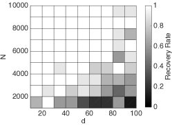
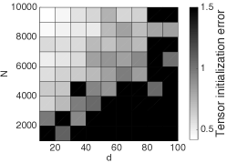
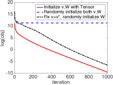
(a) Sample complexity for recovery	(b) Tensor initialization error	(c) Objective v.s. iterations

Figure 1: Numerical Experiments

6 Global Convergence

Combining the positive definiteness of the Hessian near the global optimal in Section 4 and the tensor initialization methods in Section 5, we come up with the overall globally converging algorithm Algorithm 2 and its guarantee Theorem 6.1.

Theorem 6.1 (Global convergence guarantees).

Let $S$ denote a set of i.i.d. samples from distribution ${\cal D}$ (defined in (1)) and let the activation function be homogeneous satisfying Property 3.1, 3.2, 3.3(a) and Assumption 5.3. Then for any $t\geq 1$ and any $\epsilon>0$, if $|S|\geq d\log(1/\epsilon)\cdot\operatorname{poly}(\log d,t,k,\lambda)$, $T\geq\log(1/\epsilon)\cdot\operatorname{poly}(k,\nu,\lambda,\sigma_{1}^{2p}/\rho)$ and $0<\eta\leq 1/(kv_{\max}^{2}\sigma_{1}^{2p})$, then there is an Algorithm (procedure Learning1NN in Algorithm 2) taking $|S|\cdot d\cdot\operatorname{poly}(\log d,k,\lambda)$ time and outputting a matrix $W^{(T)}\in\mathbb{R}^{d\times k}$ and a vector $v^{(0)}\in\mathbb{R}^{k}$ satisfying

$$\|W^{(T)}-W^{*}\|_{F}\leq\epsilon\|W^{*}\|_{F},\mathrm{\leavevmode\nobreak\ and\leavevmode\nobreak\ }v_{i}^{(0)}=v_{i}^{*}.$$

with probability at least $1-d^{-\Omega(t)}$.

This follows by combining Theorem 4.4 and Theorem 5.6.

7 Numerical Experiments

In this section we use synthetic data to verify our theoretical results. We generate data points $\{x_{i},y_{i}\}_{i=1,2,\cdots,n}$ from Distribution ${\cal D}$(defined in Eq. (1)). We set $W^{*}=U\Sigma V^{\top}$, where $U\in\operatorname*{{\mathbb{R}}}^{d\times k}$ and $V\in\operatorname*{{\mathbb{R}}}^{k\times k}$ are orthogonal matrices generated from QR decomposition of Gaussian matrices, $\Sigma$ is a diagonal matrix whose diagonal elements are $1,1+\frac{\kappa-1}{k-1},1+\frac{2(\kappa-1)}{k-1},\cdots,\kappa$. In this experiment, we set $\kappa=2$ and $k=5$. We set $v^{*}_{i}$ to be randomly picked from $\{-1,1\}$ with equal chance. We use squared $\mathsf{ReLU}$ $\phi(z)=\max\{z,0\}^{2}$, which is a smooth homogeneous function. For non-orthogonal tensor methods, we directly use the code provided by [KCL15] with the number of random projections fixed as $L=100$. We pick the stepsize $\eta=0.02$ for gradient descent. In the experiments, we don’t do the resampling since the algorithm still works well without resampling.

First we show the number of samples required to recover the parameters for different dimensions. We fix $k=5$, change $d$ for $d=10,20,\cdots,100$ and $n$ for $n=1000,2000,\cdots,10000$. For each pair of $d$ and $n$, we run $10$ trials. We say a trial successfully recovers the parameters if there exists a permutation $\pi:[k]\rightarrow[k]$, such that the returned parameters $W$ and $v$ satisfy

$$\max_{j\in[k]}\{\|w_{j}^{*}-w_{\pi(j)}\|/\|w_{j}^{*}\|\}\leq 0.01\text{\leavevmode\nobreak\ and\leavevmode\nobreak\ }v_{\pi(j)}=v_{j}^{*}.$$

We record the recovery rates and represent them as grey scale in Fig. 1(a). As we can see from Fig. 1(a), the least number of samples required to have 100% recovery rate is about proportional to the dimension.

Next we test the tensor initialization. We show the error between the output of the tensor method and the ground truth parameters against the number of samples under different dimensions in Fig 1(b). The pure dark blocks indicate, in at least one of the 10 trials, $\sum_{i=1}^{k}v^{{(0)}}_{i}\neq\sum_{i=1}^{k}v^{*}_{i}$, which means $v^{(0)}_{i}$ is not correctly initialized. Let $\Pi(k)$ denote the set of all possible permutations $\pi:[k]\rightarrow[k]$. The grey scale represents the averaged error,

$$\min_{\pi\in\Pi(k)}\max_{j\in[k]}\{\|w_{j}^{*}-w_{\pi(j)}^{(0)}\|/\|w_{j}^{*}\|\},$$

over 10 trials. As we can see, with a fixed dimension, the more samples we have the better initialization we obtain. We can also see that to achieve the same initialization error, the sample complexity required is about proportional to the dimension.

We also compare different initialization methods for gradient descent in Fig. 1(c). We fix $d=10,k=5,n=10000$ and compare three different initialization approaches, (i@) Let both $v$ and $W$ be initialized from tensor methods, and then do gradient descent for $W$ while $v$ is fixed; (ii@) Let both $v$ and $W$ be initialized from random Gaussian, and then do gradient descent for both $W$ and $v$; (iii@) Let $v=v^{*}$ and $W$ be initialized from random Gaussian, and then do gradient descent for $W$ while $v$ is fixed. As we can see from Fig 1(c), Approach (i@) is the fastest and Approach (ii@) doesn’t converge even if more iterations are allowed. Both Approach (i@) and (iii@) have linear convergence rate when the objective value is small enough, which verifies our local linear convergence claim.

8 Conclusion

As shown in Theorem 6.1, the tensor initialization followed by gradient descent will provide a globally converging algorithm with linear time/sample complexity in dimension, logarithmic in precision and polynomial in other factors for smooth homogeneous activation functions. Our distilled properties for activation functions include a wide range of non-linear functions and hopefully provide an intuition to understand the role of non-linear activations played in optimization. Deeper neural networks and convergence for SGD will be considered in the future.

Appendix A Notation

For any positive integer $n$, we use $[n]$ to denote the set $\{1,2,\cdots,n\}$. For random variable $X$, let $\mathbb{E}[X]$ denote the expectation of $X$ (if this quantity exists). For any vector $x\in\mathbb{R}^{n}$, we use $\|x\|$ to denote its $\ell_{2}$ norm.

We provide several definitions related to matrix $A$. Let $\det(A)$ denote the determinant of a square matrix $A$. Let $A^{\top}$ denote the transpose of $A$. Let $A^{\dagger}$ denote the Moore-Penrose pseudoinverse of $A$. Let $A^{-1}$ denote the inverse of a full rank square matrix. Let $\|A\|_{F}$ denote the Frobenius norm of matrix $A$. Let $\|A\|$ denote the spectral norm of matrix $A$. Let $\sigma_{i}(A)$ to denote the $i$-th largest singular value of $A$. We often use capital letter to denote the stack of corresponding small letter vectors, e.g., $W=[w_{1}\;w_{2}\;\cdots\;w_{k}]$. For two same-size matrices, $A,B\in\mathbb{R}^{d_{1}\times d_{2}}$, we use $A\circ B\in\mathbb{R}^{d_{1}\times d_{2}}$ to denote element-wise multiplication of these two matrices.

We use $\otimes$ to denote outer product and $\cdot$ to denote dot product. Given two column vectors $u,v\in\mathbb{R}^{n}$, then $u\otimes v\in\mathbb{R}^{n\times n}$ and $(u\otimes v)_{i,j}=u_{i}\cdot v_{j}$, and $u^{\top}v=\sum_{i=1}^{n}u_{i}v_{i}\in\mathbb{R}$. Given three column vectors $u,v,w\in\mathbb{R}^{n}$, then $u\otimes v\otimes w\in\mathbb{R}^{n\times n\times n}$ and $(u\otimes v\otimes w)_{i,j,k}=u_{i}\cdot v_{j}\cdot w_{k}$. We use $u^{\otimes r}\in\mathbb{R}^{n^{r}}$ to denote the vector $u$ outer product with itself $r-1$ times.

Tensor $T\in\mathbb{R}^{n\times n\times n}$ is symmetric if and only if for any $i,j,k$, $T_{i,j,k}=T_{i,k,j}=T_{j,i,k}=T_{j,k,i}=T_{k,i,j}$ $=T_{k,j,i}$. Given a third order tensor $T\in\mathbb{R}^{n_{1}\times n_{2}\times n_{3}}$ and three matrices $A\in\mathbb{R}^{n_{1}\times d_{1}},B\in\mathbb{R}^{n_{2}\times d_{2}},C\in\mathbb{R}^{n_{3}\times d_{3}}$, we use $T(A,B,C)$ to denote a $d_{1}\times d_{2}\times d_{3}$ tensor where the $(i,j,k)$-th entry is,

$$\overset{n_{1}}{\underset{i^{\prime}=1}{\sum}}\overset{n_{2}}{\underset{j^{\prime}=1}{\sum}}\overset{n_{3}}{\underset{k^{\prime}=1}{\sum}}T_{i^{\prime},j^{\prime},k^{\prime}}A_{i^{\prime},i}B_{j^{\prime},j}C_{k^{\prime},k}.$$

We use $\|T\|$ to denote the operator norm of the tensor $T$, i.e.,

$$\|T\|=\underset{\|a\|=1}{\max}|T(a,a,a)|.$$

For tensor $T\in\mathbb{R}^{n_{1}\times n_{2}\times n_{3}}$, we use matrix $T^{(1)}\in\mathbb{R}^{n_{1}\times n_{2}n_{3}}$ to denote the flattening of tensor $T$ along the first dimension, i.e., $[T^{(1)}]_{i,(j-1)n_{3}+k}=T_{i,j,k},\forall i\in[n_{1}],j\in[n_{2}],k\in[n_{3}]$. Similarly for matrices $T^{(2)}\in\mathbb{R}^{n_{2}\times n_{3}n_{1}}$ and $T^{(3)}\in\mathbb{R}^{n_{3}\times n_{1}n_{2}}$.

We use ${\mathbf{1}}_{f}$ to denote the indicator function, which is $1$ if $f$ holds and $0$ otherwise. Let $I_{d}\in\mathbb{R}^{d\times d}$ denote the identity matrix. We use $\phi(z)$ to denote an activation function. We define $(z)_{+}:=\max\{0,z\}$. We use ${\cal D}$ to denote a Gaussian distribution ${\cal N}(0,I_{d})$ or to denote a joint distribution of $(X,Y)\in\mathbb{R}^{d}\times\mathbb{R}$, where the marginal distribution of $X$ is ${\cal N}(0,I_{d})$.

For any function $f$, we define $\widetilde{O}(f)$ to be $f\cdot\log^{O(1)}(f)$. In addition to $O(\cdot)$ notation, for two functions $f,g$, we use the shorthand $f\lesssim g$ (resp. $\gtrsim$) to indicate that $f\leq Cg$ (resp. $\geq$) for an absolute constant $C$. We use $f\eqsim g$ to mean $cf\leq g\leq Cf$ for constants $c,C$.

Appendix B Preliminaries

In this section, we introduce some lemmata and corollaries that will be used in the proofs.

B.1 Useful Facts

We provide some facts that will be used in the later proofs.

Fact B.1.

Let $z$ denote a fixed $d$-dimensional vector, then for any $C\geq 1$ and $n\geq 1$, we have

$$\underset{x\sim{\cal N}(0,I_{d})}{\Pr}[|\langle x,z\rangle|^{2}\leq 5C\|z\|^{2}\log n]\geq 1-1/(nd^{C}).$$

Proof.

This follows by Proposition 1.1 in [HKZ12]. ∎

Fact B.2.

For any $C\geq 1$ and $n\geq 1$, we have

$$\underset{x\sim{\cal N}(0,I_{d})}{\Pr}[\|x\|^{2}\leq 5Cd\log n]\geq 1-1/(nd^{C}).$$

Proof.

This follows by Proposition 1.1 in [HKZ12]. ∎

Fact B.3.

Given a full column-rank matrix $W=[w_{1},w_{2},\cdots,w_{k}]\in\mathbb{R}^{d\times k}$, let $\overline{W}=[\frac{w_{1}}{\|w_{1}\|}$, $\frac{w_{2}}{\|w_{2}\|}$, $\cdots$, $\frac{w_{k}}{\|w_{k}\|}]$. Then, we have: (i@) for any $i\in[k]$, $\sigma_{k}(W)\leq\|w_{i}\|\leq\sigma_{1}(W)$; (ii@) $1/\kappa(W)\leq\sigma_{k}(\overline{W})\leq\sigma_{1}(\overline{W})\leq\sqrt{k}$.

Proof.

Part (i@). We have,

$$\sigma_{k}(W)\leq\|We_{i}\|=\|w_{i}\|\leq\sigma_{1}(W)$$

Part (ii@). We first show how to lower bound $\sigma_{k}(\overline{W})$,

$$\sigma_{k}(\overline{W}) =\leavevmode\nobreak\ \min_{\|s\|=1}\|\overline{W}s\|$$

$$=\leavevmode\nobreak\ \min_{\|s\|=1}\left\|\sum_{i=1}^{k}\frac{s_{i}}{\|w_{i}\|}w_{i}\right\| \text{\leavevmode\nobreak\ by\leavevmode\nobreak\ definition\leavevmode\nobreak\ of\leavevmode\nobreak\ }\overline{W}$$

$$\geq\leavevmode\nobreak\ \min_{\|s\|=1}\sigma_{k}(W)\left(\sum_{i=1}^{k}(\frac{s_{i}}{\|w_{i}\|})^{2}\right)^{\frac{1}{2}} \text{\leavevmode\nobreak\ by\leavevmode\nobreak\ }\|w_{i}\|\geq\sigma_{k}(W)$$

$$\geq\leavevmode\nobreak\ \min_{\|s\|_{2}=1}\sigma_{k}(W)\left(\sum_{i=1}^{k}(\frac{s_{i}}{\max_{j\in[k]}\|w_{j}\|})^{2}\right)^{\frac{1}{2}} \text{\leavevmode\nobreak\ by\leavevmode\nobreak\ }\max_{j\in[k]}\|w_{j}\|\geq\|w_{i}\|$$

$$=\leavevmode\nobreak\ \sigma_{k}(W)/\max_{j\in[k]}\|w_{j}\| \text{\leavevmode\nobreak\ by\leavevmode\nobreak\ }\|s\|=1$$

$$\geq\leavevmode\nobreak\ \sigma_{k}(W)/\sigma_{1}(W). \text{\leavevmode\nobreak\ by\leavevmode\nobreak\ }\max_{j\in[k]}\|w_{j}\|\leq\sigma_{1}(W)$$

$$=\leavevmode\nobreak\ 1/\kappa(W).$$

It remains to upper bound $\sigma_{1}(\overline{W})$,

$$\sigma_{1}(\overline{W})\leq\left(\sum_{i=1}^{k}\sigma_{i}^{2}(\overline{W})\right)^{\frac{1}{2}}=\|\overline{W}\|_{F}\leq\sqrt{k}.$$

∎

Fact B.4.

Let $U\in\operatorname*{{\mathbb{R}}}^{d\times k}$ and $V\in\operatorname*{{\mathbb{R}}}^{d\times k}$ $(k\leq d)$ denote two orthogonal matrices. Then $\|UU^{\top}-VV^{\top}\|=\|(I-UU^{\top})V\|=\|(I-VV^{\top})U\|=\sqrt{1-\sigma_{k}^{2}(U^{\top}V)}$.

Proof.

Let $U_{\perp}\in\mathbb{R}^{d\times(d-k)}$ and $V_{\perp}\in\mathbb{R}^{d\times(d-k)}$ be the orthogonal complementary matrices of $U,V\in\mathbb{R}^{d\times k}$ respectively.

$$\|UU^{\top}-VV^{\top}\| =\|(I-VV^{\top})UU^{\top}-VV^{\top}(I-UU^{\top})\|$$

$$=\|V_{\perp}V_{\perp}^{\top}UU^{\top}-VV^{\top}U_{\perp}U_{\perp}^{\top}\|$$

$$=\left\|\begin{bmatrix}V_{\perp}&V\end{bmatrix}\begin{bmatrix}V_{\perp}^{\top}U&0\\ 0&-V^{\top}U_{\perp}\end{bmatrix}\begin{bmatrix}U^{\top}\\ U_{\perp}^{\top}\end{bmatrix}\right\|$$

$$=\max(\|V_{\perp}^{\top}U\|,\|V^{\top}U_{\perp}\|).$$

We show how to simplify $\|V_{\perp}^{\top}U\|$,

$$\|V_{\perp}^{\top}U\|=\|(I-VV^{\top})U\|=\sqrt{\|U^{\top}(I-VV^{\top})U\|}=\max_{\|a\|=1}\sqrt{1-\|V^{\top}Ua\|^{2}}=\sqrt{1-\sigma_{k}^{2}(V^{\top}U)}.$$

Similarly we can simplify $\|U_{\perp}^{\top}V\|$,

$$\|U_{\perp}^{\top}V\|=\sqrt{1-\sigma^{2}_{k}(U^{\top}V)}=\sqrt{1-\sigma^{2}_{k}(V^{\top}U)}.$$

∎

Fact B.5.

Let $C\in\operatorname*{{\mathbb{R}}}^{d_{1}\times d_{2}},B\in\operatorname*{{\mathbb{R}}}^{d_{2}\times d_{3}}$ be two matrices. Then $\|CB\|\leq\|C\|\|B\|_{F}$ and $\|CB\|\geq\sigma_{\min}(C)\|B\|_{F}$.

Proof.

For each $i\in[d_{3}]$, let $b_{i}$ denote the $i$-th column of $B$. We can upper bound $\|CB\|$,

$$\|CB\|_{F}=\left(\sum_{i=1}^{d_{2}}\|Cb_{i}\|^{2}\right)^{1/2}\leq\left(\sum_{i=1}^{d_{2}}\|C\|^{2}\|b_{i}\|^{2}\right)^{1/2}=\|C\|\|B\|_{F}.$$

We show how to lower bound $\|CB\|$,

$$\|CB\|=\left(\sum_{i=1}^{d_{2}}\|Cb_{i}\|^{2}\right)^{1/2}\geq\left(\sum_{i=1}^{d_{2}}\sigma_{k}^{2}(C)\|b_{i}\|^{2}\right)^{1/2}=\sigma_{\min}(C)\|B\|_{F}.$$

∎

Fact B.6.

Let $a,b,c\geq 0$ denote three constants, let $u,v,w\in\mathbb{R}^{d}$ denote three vectors, let ${\cal D}_{d}$ denote Gaussian distribution ${\cal N}(0,I_{d})$ then

$$\underset{x\sim{\cal D}_{d}}{\operatorname*{{\mathbb{E}}}}\left[|u^{\top}x|^{a}|v^{\top}x|^{b}|w^{\top}x|^{c}\right]\eqsim\|u\|^{a}\|v\|^{b}\|w\|^{c}.$$

Proof.

$$\underset{x\sim{\cal D}_{d}}{\operatorname*{{\mathbb{E}}}}\left[|u^{\top}x|^{a}|v^{\top}x|^{b}|w^{\top}x|^{c}\right]\leq \leavevmode\nobreak\ \left(\underset{x\sim{\cal D}_{d}}{\operatorname*{{\mathbb{E}}}}[|u^{\top}x|^{2a}]\right)^{1/2}\cdot\left(\underset{x\sim{\cal D}_{d}}{\operatorname*{{\mathbb{E}}}}[|u^{\top}x|^{4b}]\right)^{1/4}\cdot\left(\underset{x\sim{\cal D}_{d}}{\operatorname*{{\mathbb{E}}}}[|u^{\top}x|^{4c}]\right)^{1/4}$$

$$\lesssim \leavevmode\nobreak\ \|u\|^{a}\|v\|^{b}\|w\|^{c},$$

where the first step follows by Hölder’s inequality, i.e., $\operatorname*{{\mathbb{E}}}[|XYZ|]\leq(\operatorname*{{\mathbb{E}}}[|X|^{2}])^{1/2}\cdot(\operatorname*{{\mathbb{E}}}[|Y|^{4}])^{1/4}\cdot(\operatorname*{{\mathbb{E}}}[|Z|^{4}])^{1/4}$, the third step follows by calculating the expectation and $a,b,c$ are constants.

Since all the three components $|u^{\top}x|$, $|v^{\top}x|$, $|w^{\top}x|$ are positive and related to a common random vector $x$, we can show a lower bound,

$$\underset{x\sim{\cal D}_{d}}{\operatorname*{{\mathbb{E}}}}\left[|u^{\top}x|^{a}|v^{\top}x|^{b}|w^{\top}x|^{c}\right]\gtrsim\|u\|^{a}\|v\|^{b}\|w\|^{c}.$$

∎

B.2 Matrix Bernstein

In many proofs we need to bound the difference between some population matrices/tensors and their empirical versions. Typically, the classic matrix Bernstein inequality requires the norm of the random matrix be bounded almost surely (e.g., Theorem 6.1 in [Tro12]) or the random matrix satisfies subexponential property (Theorem 6.2 in [Tro12]) . However, in our cases, most of the random matrices don’t satisfy these conditions. So we derive the following lemmata that can deal with random matrices that are not bounded almost surely or follow subexponential distribution, but are bounded with high probability.

Lemma B.7 (Matrix Bernstein for unbounded case (A modified version of bounded case, Theorem 6.1 in [Tro12])).

Let ${\cal B}$ denote a distribution over $\mathbb{R}^{d_{1}\times d_{2}}$. Let $d=d_{1}+d_{2}$. Let $B_{1},B_{2},\cdots B_{n}$ be i.i.d. random matrices sampled from ${\cal B}$. Let $\overline{B}=\mathbb{E}_{B\sim{\cal B}}[B]$ and $\widehat{B}=\frac{1}{n}\sum_{i=1}^{n}B_{i}$. For parameters $m\geq 0,\gamma\in(0,1),\nu>0,L>0$, if the distribution ${\cal B}$ satisfies the following four properties,

$$\mathrm{(\@slowromancap i@)}\quad \quad\underset{B\sim{\cal B}}{\Pr}\left[\left\|B\right\|\leq m\right]\geq 1-\gamma;$$

$$\mathrm{(\@slowromancap ii@)}\quad \quad\left\|\underset{B\sim{\cal B}}{\mathbb{E}}[B]\right\|>0;$$

$$\mathrm{(\@slowromancap iii@)}\quad \quad\max\left(\left\|\underset{B\sim{\cal B}}{\mathbb{E}}[BB^{\top}]\right\|,\left\|\underset{B\sim{\cal B}}{\mathbb{E}}[B^{\top}B]\right\|\right)\leq\nu;$$

$$\mathrm{(\@slowromancap iv@)}\quad \quad\max_{\|a\|=\|b\|=1}\left(\underset{B\sim{\cal B}}{\mathbb{E}}\left[\left(a^{\top}Bb\right)^{2}\right]\right)^{1/2}\leq L.$$

Then we have for any $0<\epsilon<1$ and $t\geq 1$, if

$$n\geq(18t\log d)\cdot(\nu+\|\overline{B}\|^{2}+m\|\overline{B}\|\epsilon)/(\epsilon^{2}\|\overline{B}\|^{2})\quad\text{\leavevmode\nobreak\ and\leavevmode\nobreak\ }\quad\gamma\leq(\epsilon\|\overline{B}\|/(2L))^{2}$$

with probability at least $1-1/d^{2t}-n\gamma$,

$$\|\widehat{B}-\overline{B}\|\leq\epsilon\|\overline{B}\|.$$

Proof.

Define the event

$$\xi_{i}=\{\|B_{i}\|\leq m\},\forall i\in[n].$$

Define $M_{i}={\mathbf{1}}_{\|B_{i}\|\leq m}B_{i}$. Let $\overline{M}=\mathbb{E}_{B\sim{\cal B}}[{\mathbf{1}}_{\|B\|\leq m}B]$ and $\widehat{M}=\frac{1}{n}\sum_{i=1}^{n}M_{i}$. By triangle inequality, we have

$$\|\widehat{B}-\overline{B}\|\leq\|\widehat{B}-\widehat{M}\|+\|\widehat{M}-\overline{M}\|+\|\overline{M}-\overline{B}\|.$$ (4)

In the next a few paragraphs, we will upper bound the above three terms.

The first term in Eq. (4). Denote $\xi^{c}$ as the complementary set of $\xi$, thus $\Pr[\xi^{c}_{i}]\leq\gamma$. By a union bound over $i\in[n]$, with probability $1-n\gamma$, $\|B_{i}\|\leq m$ for all $i\in[n]$. Thus $\widehat{M}=\widehat{B}$.

The second term in Eq. (4). For a matrix $B$ sampled from ${\cal B}$, we use $\xi$ to denote the event that $\xi=\{\|B\|\leq m\}$. Then, we can upper bound $\|\overline{M}-\overline{B}\|$ in the following way,

$$\leavevmode\nobreak\ \|\overline{M}-\overline{B}\|$$

$$= \leavevmode\nobreak\ \left\|\underset{B\sim{\cal B}}{\mathbb{E}}[{\mathbf{1}}_{\|B\|\leq m}\cdot B]-\underset{B\sim{\cal B}}{\mathbb{E}}[B]\right\|$$

$$= \leavevmode\nobreak\ \left\|\underset{B\sim{\cal B}}{\mathbb{E}}[B\cdot{\mathbf{1}}_{\xi^{c}}]\right\|$$

$$= \leavevmode\nobreak\ \max_{\|a\|=\|b\|=1}\underset{B\sim{\cal B}}{\mathbb{E}}[a^{\top}Bb{\mathbf{1}}_{\xi^{c}}]$$

$$\leq \leavevmode\nobreak\ \max_{\|a\|=\|b\|=1}\underset{B\sim{\cal B}}{\mathbb{E}}[(a^{\top}Bb)^{2}]^{1/2}\cdot\underset{B\sim{\cal B}}{\mathbb{E}}[{\mathbf{1}}_{\xi^{c}}]^{1/2}$$  by Hölder’s inequality

$$\leq \leavevmode\nobreak\ L\underset{B\sim{\cal B}}{\mathbb{E}}[{\mathbf{1}}_{\xi^{c}}]^{1/2}$$  by Property (iv@)

$$\leq \leavevmode\nobreak\ L\gamma^{1/2}, \text{\leavevmode\nobreak\ by\leavevmode\nobreak\ }\Pr[\xi^{c}]\leq\gamma$$

$$\leq \leavevmode\nobreak\ \frac{1}{2}\epsilon\|\overline{B}\|, \text{\leavevmode\nobreak\ by\leavevmode\nobreak\ }\gamma\leq(\epsilon\|\overline{B}\|/(2L))^{2}$$

which implies

$$\|\overline{M}-\overline{B}\|\leq\frac{\epsilon}{2}\|\overline{B}\|.$$

Since $\epsilon<1$, we also have $\|\overline{M}-\overline{B}\|\leq\frac{1}{2}\|\overline{B}\|$ and $\frac{3}{2}\|\overline{B}\|\geq\|\overline{M}\|\geq\frac{1}{2}\|\overline{B}\|$.

The third term in Eq. (4). We can bound $\|\widehat{M}-\overline{M}\|$ by Matrix Bernstein’s inequality [Tro12].

We define $Z_{i}=M_{i}-\overline{M}$. Thus we have $\underset{B_{i}\sim{\cal B}}{\mathbb{E}}[Z_{i}]=0$, $\|Z_{i}\|\leq 2m$, and

$$\left\|\underset{B_{i}\sim{\cal B}}{\mathbb{E}}[Z_{i}Z_{i}^{\top}]\right\|=\left\|\underset{B_{i}\sim{\cal B}}{\mathbb{E}}[M_{i}M_{i}^{\top}]-\overline{M}\cdot\overline{M}^{\top}\right\|\leq\nu+\|\overline{M}\|^{2}\leq\nu+3\|\overline{B}\|^{2}.$$

Similarly, we have $\left\|\underset{B_{i}\sim{\cal B}}{\mathbb{E}}[Z_{i}^{\top}Z_{i}]\right\|\leq\nu+3\|\overline{B}\|^{2}$. Using matrix Bernstein’s inequality, for any $\epsilon>0$,

$$\underset{B_{1},\cdots,B_{n}\sim{\cal B}}{\Pr}\left[\frac{1}{n}\left\|\sum_{i=1}^{n}Z_{i}\right\|\geq\epsilon\|\overline{B}\|\right]\leq d\exp\left(-\frac{\epsilon^{2}\|\overline{B}\|^{2}n/2}{\nu+3\|\overline{B}\|^{2}+2m\|\overline{B}\|\epsilon/3}\right).$$

By choosing

$$n\geq(3t\log d)\cdot\frac{\nu+3\|\overline{B}\|^{2}+2m\|\overline{B}\|\epsilon/3}{\epsilon^{2}\|\overline{B}\|^{2}/2},$$

for $t\geq 1$, we have with probability at least $1-1/d^{2t}$,

$$\left\|\frac{1}{n}\sum_{i=1}^{n}M_{i}-\overline{M}\right\|\leq\frac{\epsilon}{2}\|\overline{B}\|$$

Putting it all together, we have for $0<\epsilon<1$, if

$$n\geq(18t\log d)\cdot(\nu+\|\overline{B}\|^{2}+m\|\overline{B}\|\epsilon)/(\epsilon^{2}\|\overline{B}\|^{2})\quad\text{\leavevmode\nobreak\ and\leavevmode\nobreak\ }\quad\gamma\leq(\epsilon\|\overline{B}\|/(2L))^{2}$$

with probability at least $1-1/d^{2t}-n\gamma$,

$$\left\|\frac{1}{n}\sum_{i=1}^{n}B_{i}-\underset{B\sim{\cal B}}{\mathbb{E}}[B]\right\|\leq\epsilon\left\|\underset{B\sim{\cal B}}{\mathbb{E}}[B]\right\|.$$

∎

Corollary B.8 (Error bound for symmetric rank-one random matrices).

Let $x_{1},x_{2},\cdots x_{n}$ denote $n$ i.i.d. samples drawn from Gaussian distribution ${\cal N}(0,I_{d})$. Let $h(x):\mathbb{R}^{d}\rightarrow\mathbb{R}$ be a function satisfying the following properties $\mathrm{(\@slowromancap i@)}$, $\mathrm{(\@slowromancap ii@)}$ and $\mathrm{(\@slowromancap iii@)}$.

$$\mathrm{(\@slowromancap i@)}\leavevmode\nobreak\ \leavevmode\nobreak\ \underset{x\sim{\cal N}(0,I_{d})}{\Pr}\left[|h(x)|\leq m\right]\geq 1-\gamma$$

$$\mathrm{(\@slowromancap ii@)}\leavevmode\nobreak\ \leavevmode\nobreak\ \left\|\underset{x\sim{\cal N}(0,I_{d})}{\mathbb{E}}[h(x)xx^{\top}]\right\|>0;$$

$$\mathrm{(\@slowromancap iii@)}\leavevmode\nobreak\ \leavevmode\nobreak\ \left(\underset{x\sim{\cal N}(0,I_{d})}{\mathbb{E}}[h^{4}(x)]\right)^{1/4}\leq L.$$

Define function $B(x)=h(x)xx^{\top}\in\mathbb{R}^{d\times d}$, $\forall i\in[n]$. Let $\overline{B}=\underset{x\sim{\cal N}(0,I_{d})}{\mathbb{E}}[h(x)xx^{\top}]$. For any $0<\epsilon<1$ and $t\geq 1$, if

$$n\gtrsim(t\log d)\cdot(L^{2}d+\|\overline{B}\|^{2}+(mtd\log n)\|\overline{B}\|\epsilon)/(\epsilon^{2}\|\overline{B}\|^{2}),\text{\leavevmode\nobreak\ and\leavevmode\nobreak\ }\gamma+1/(nd^{2t})\lesssim(\epsilon\|\overline{B}\|/L)^{2}$$

then

$$\underset{x_{1},\cdots,x_{n}\sim{\cal N}(0,I_{d})}{\Pr}\left[\left\|\overline{B}-\frac{1}{n}\sum_{i=1}^{n}B(x_{i})\right\|\leq\epsilon\|\overline{B}\|\right]\geq 1-2/(d^{2t})-n\gamma.$$

Proof.

We show that the four Properties in Lemma B.7 are satisfied. Define function $B(x)=h(x)xx^{\top}$.

(i@) $\|B(x)\|=\|h(x)xx^{\top}\|=|h(x)|\|x\|^{2}$.

By using Fact B.2, we have

$$\underset{x\sim{\cal N}(0,I_{d})}{\Pr}[\|x\|^{2}\leq 10td\log n]\geq 1-1/(nd^{2t})$$

Therefore,

$$\underset{x\sim{\cal N}(0,I_{d})}{\Pr}[\|B(x)\|\leq m\cdot 10td\log(n)]\geq 1-\gamma-1/(nd^{2t}).$$

(ii@) $\left\|\underset{B\sim{\cal B}}{\operatorname*{{\mathbb{E}}}}[B]\right\|=\left\|\underset{x\sim{\cal N}(0,I_{d})}{\operatorname*{{\mathbb{E}}}}[h(x)xx^{\top}]\right\|>0$.

(iii@)

$$\leavevmode\nobreak\ \max\left(\left\|\underset{B\sim{\cal B}}{\operatorname*{{\mathbb{E}}}}[BB^{\top}]\right\|,\left\|\underset{B\sim{\cal B}}{\operatorname*{{\mathbb{E}}}}[B^{\top}B]\right\|\right)$$

$$= \leavevmode\nobreak\ \max_{\|a\|=1}\underset{x\sim{\cal N}(0,I_{d})}{\operatorname*{{\mathbb{E}}}}[(h(x))^{2}\|x\|^{2}(a^{\top}x)^{2}]$$

$$\leq \leavevmode\nobreak\ \left(\underset{x\sim{\cal N}(0,I_{d})}{\operatorname*{{\mathbb{E}}}}[(h(x))^{4}]\right)^{1/2}\cdot\left(\underset{x\sim{\cal N}(0,I_{d})}{\operatorname*{{\mathbb{E}}}}[\|x\|^{8}]\right)^{1/4}\cdot\max_{\|a\|=1}\left(\underset{x\sim{\cal N}(0,I_{d})}{\operatorname*{{\mathbb{E}}}}[(a^{\top}x)^{8}]\right)^{1/4}$$

$$\lesssim \leavevmode\nobreak\ L^{2}d.$$

(iv@)

$$\leavevmode\nobreak\ \max_{\|a\|=\|b\|=1}\left(\underset{B\sim{\cal B}}{\operatorname*{{\mathbb{E}}}}[(a^{\top}Bb)^{2}]\right)^{1/2}$$

$$= \leavevmode\nobreak\ \max_{\|a\|=1}\left(\underset{x\sim{\cal N}(0,I_{d})}{\operatorname*{{\mathbb{E}}}}[h^{2}(x)(a^{\top}x)^{4}]\right)^{1/2}$$

$$\leq \leavevmode\nobreak\ \left(\underset{x\sim{\cal N}(0,I_{d})}{\operatorname*{{\mathbb{E}}}}[h^{4}(x)]\right)^{1/4}\cdot\max_{\|a\|=1}\left(\underset{x\sim{\cal N}(0,I_{d})}{\operatorname*{{\mathbb{E}}}}[(a^{\top}x)^{8}]\right)^{1/4}$$

$$\lesssim \leavevmode\nobreak\ L.$$

Applying Lemma B.7, we obtain, for any $0<\epsilon<1$ and $t\geq 1$, if

$$n\gtrsim(t\log d)\cdot(L^{2}d+\|\overline{B}\|^{2}+(mtd\log n)\|\overline{B}\|\epsilon)/(\epsilon^{2}\|\overline{B}\|^{2}),\text{\leavevmode\nobreak\ and\leavevmode\nobreak\ }\gamma+1/(nd^{2t})\lesssim(\epsilon\|\overline{B}\|/L)^{2}$$

then

$$\underset{x_{1},\cdots,x_{n}\sim{\cal N}(0,I_{d})}{\Pr}\left[\left\|\overline{B}-\frac{1}{n}\sum_{i=1}^{n}B(x_{i})\right\|\leq\epsilon\|\overline{B}\|\right]\geq 1-2/(d^{2t})-n\gamma.$$

∎

Appendix C Properties of Activation Functions

Theorem 3.5.

$\mathsf{ReLU}$ $\phi(z)=\max\{z,0\}$, leaky $\mathsf{ReLU}$ $\phi(z)=\max\{z,0.01z\}$, squared $\mathsf{ReLU}$ $\phi(z)=\max\{z,0\}^{2}$ and any non-linear non-decreasing smooth functions with bounded symmetric $\phi^{\prime}(z)$, like the sigmoid function $\phi(z)=1/(1+e^{-z})$, the $\mathrm{tanh}$ function and the $\mathrm{erf}$ function $\phi(z)=\int_{0}^{z}e^{-t^{2}}dt$, satisfy Property 3.1,3.2,3.3. The linear function, $\phi(z)=z$, doesn’t satisfy Property 3.2 and the quadratic function, $\phi(z)=z^{2}$, doesn’t satisfy Property 3.1 and 3.2.

Proof.

We can easily verify that $\mathsf{ReLU}$ , leaky $\mathsf{ReLU}$ and squared $\mathsf{ReLU}$ satisfy Property 3.2 by calculating $\rho(\sigma)$ in Property 3.2, which is shown in Table 1. Property 3.1 for $\mathsf{ReLU}$ , leaky $\mathsf{ReLU}$ and squared $\mathsf{ReLU}$ can be verified since they are non-decreasing with bounded first derivative. $\mathsf{ReLU}$ and leaky $\mathsf{ReLU}$ are piece-wise linear, so they satisfy Property 3.3(b). Squared $\mathsf{ReLU}$ is smooth so it satisfies Property 3.3(a).

Activations	$\mathsf{ReLU}$	Leaky $\mathsf{ReLU}$	squared $\mathsf{ReLU}$	erf	sigmoid ($\sigma=0.1$)	sigmoid ($\sigma=1$)	sigmoid ($\sigma=10$)
$\alpha_{0}(\sigma)$	$\frac{1}{2}$	$\frac{1.01}{2}$	$\sigma\sqrt{\frac{2}{\pi}}$	$\frac{1}{(2\sigma^{2}+1)^{1/2}}$	0.99	0.605706	0.079
$\alpha_{1}(\sigma)$	$\frac{1}{\sqrt{2\pi}}$	$\frac{0.99}{\sqrt{2\pi}}$	$\sigma$	0	0	0	0
$\alpha_{2}(\sigma)$	$\frac{1}{2}$	$\frac{1.01}{2}$	$2\sigma\sqrt{\frac{2}{\pi}}$	$\frac{1}{(2\sigma^{2}+1)^{3/2}}$	0.97	0.24	0.00065
$\beta_{0}(\sigma)$	$\frac{1}{2}$	$\frac{1.0001}{2}$	$2\sigma$	$\frac{1}{(4\sigma^{2}+1)^{1/2}}$	0.98	0.46	0.053
$\beta_{2}(\sigma)$	$\frac{1}{2}$	$\frac{1.0001}{2}$	$6\sigma$	$\frac{1}{(4\sigma^{2}+1)^{3/2}}$	0.94	0.11	0.00017
$\rho(\sigma)$	0.091	0.089	0.27$\sigma$	$\rho_{\text{erf}}(\sigma)$ 1	1.8E-4	4.9E-2	5.1E-5

Table 1: $\rho(\sigma)$ values for different activation functions. Note that we can calculate the exact values for $\mathsf{ReLU}$, Leaky $\mathsf{ReLU}$, squared $\mathsf{ReLU}$ and erf. We can’t find a closed-form value for sigmoid or tanh, but we calculate the numerical values of $\rho(\sigma)$ for $\sigma=0.1,1,10$. ¹ $\rho_{\text{erf}}(\sigma)=\min\{(4\sigma^{2}+1)^{-1/2}-(2\sigma^{2}+1)^{-1},(4\sigma^{2}+1)^{-3/2}-(2\sigma^{2}+1)^{-3},(2\sigma^{2}+1)^{-2}\}$

Smooth non-decreasing activations with bounded first derivatives automatically satisfy Property 3.1 and  3.3. For Property 3.2, since their first derivatives are symmetric, we have $\operatorname*{{\mathbb{E}}}[\phi^{\prime}(\sigma\cdot z)z]=0$. Then by Hölder’s inequality and $\phi^{\prime}(z)\geq 0$, we have

$$\operatorname*{{\mathbb{E}}}_{z\sim\operatorname*{{\mathcal{D}}}_{1}}[\phi^{\prime 2}(\sigma\cdot z)]\geq\left(\operatorname*{{\mathbb{E}}}_{z\sim\operatorname*{{\mathcal{D}}}_{1}}[\phi^{\prime}(\sigma\cdot z)]\right)^{2},$$

$$\operatorname*{{\mathbb{E}}}_{z\sim\operatorname*{{\mathcal{D}}}_{1}}[\phi^{\prime 2}(\sigma\cdot z)z^{2}]\cdot\operatorname*{{\mathbb{E}}}_{z\sim\operatorname*{{\mathcal{D}}}_{1}}[z^{2}]\geq\left(\operatorname*{{\mathbb{E}}}_{z\sim\operatorname*{{\mathcal{D}}}_{1}}[\phi^{\prime}(\sigma\cdot z)z^{2}]\right)^{2},$$

$$\operatorname*{{\mathbb{E}}}_{z\sim\operatorname*{{\mathcal{D}}}_{1}}[\phi^{\prime}(\sigma\cdot z)z^{2}]\cdot\operatorname*{{\mathbb{E}}}_{z\sim\operatorname*{{\mathcal{D}}}_{1}}[\phi^{\prime}(\sigma\cdot z)]=\operatorname*{{\mathbb{E}}}_{z\sim\operatorname*{{\mathcal{D}}}_{1}}[(\sqrt{\phi^{\prime}(\sigma\cdot z)}z)^{2}]\cdot\operatorname*{{\mathbb{E}}}_{z\sim\operatorname*{{\mathcal{D}}}_{1}}[(\sqrt{\phi^{\prime}(\sigma\cdot z)})^{2}]\geq\left(\operatorname*{{\mathbb{E}}}_{z\sim\operatorname*{{\mathcal{D}}}_{1}}[\phi^{\prime}(\sigma\cdot z)z]\right)^{2}.$$

The equality in the first inequality happens when $\phi^{\prime}(\sigma\cdot z)$ is a constant a.e.. The equality in the second inequality happens when $|\phi^{\prime}(\sigma\cdot z)|$ is a constant a.e., which is invalidated by the non-linearity and smoothness condition. The equality in the third inequality holds only when $\phi^{\prime}(z)=0$ a.e., which leads to a constant function under non-decreasing condition. Therefore, $\rho(\sigma)>0$ for any smooth non-decreasing non-linear activations with bounded symmetric first derivatives. The statements about linear activations and quadratic activation follow direct calculations. ∎

Appendix D Local Positive Definiteness of Hessian

D.1 Main Results for Positive Definiteness of Hessian

D.1.1 Bounding the Spectrum of the Hessian near the Ground Truth

Theorem D.1 (Bounding the spectrum of the Hessian near the ground truth).

For any $W\in\mathbb{R}^{d\times k}$ with $\|W-W^{*}\|\lesssim v_{\min}^{4}\rho^{2}(\sigma_{k})/(k^{2}\kappa^{5}{\lambda}^{2}v_{\max}^{4}\sigma_{1}^{4p})\cdot\|W^{*}\|$, let $S$ denote a set of i.i.d. samples from distribution ${\cal D}$ (defined in (1)) and let the activation function satisfy Property 3.1,3.2,3.3. Then for any $t\geq 1$, if $|S|\geq d\cdot\operatorname{poly}(\log d,t)\cdot k^{2}v_{\max}^{4}\tau\kappa^{8}\lambda^{2}\sigma_{1}^{4p}/(v_{\min}^{4}\rho^{2}(\sigma_{k}))$, we have with probability at least $1-d^{-\Omega(t)}$,

$$\Omega(v_{\min}^{2}\rho(\sigma_{k})/(\kappa^{2}\lambda))I\preceq\nabla^{2}\widehat{f}_{S}(W)\preceq O(kv_{\max}^{2}\sigma_{1}^{2p})I.$$

Proof.

The main idea of the proof follows the following inequalities,

$$\nabla^{2}f_{\cal D}(W^{*})-\|\nabla^{2}\widehat{f}_{S}(W)-\nabla^{2}f_{\cal D}(W^{*})\|I\preceq\nabla^{2}\widehat{f}_{S}(W)\preceq\leavevmode\nobreak\ \nabla^{2}f_{\cal D}(W^{*})+\|\nabla^{2}\widehat{f}_{S}(W)-\nabla^{2}f_{\cal D}(W^{*})\|I$$

The proof sketch is first to bound the range of the eigenvalues of $\nabla^{2}f_{\cal D}(W^{*})$ (Lemma D.3) and then bound the spectral norm of the remaining error, $\|\nabla^{2}\widehat{f}_{S}(W)-\nabla^{2}f_{\cal D}(W^{*})\|$. $\|\nabla^{2}\widehat{f}_{S}(W)-\nabla^{2}f_{\cal D}(W^{*})\|$ can be further decomposed into two parts, $\|\nabla^{2}\widehat{f}_{S}(W)-H\|$ and $\|H-\nabla^{2}f_{\cal D}(W^{*})\|$, where $H$ is $\nabla^{2}f_{\cal D}(W)$ if $\phi$ is smooth, otherwise $H$ is a specially designed matrix . We can upper bound them when $W$ is close enough to $W^{*}$ and there are enough samples. In particular, if the activation satisfies Property 3.3(a), see Lemma D.10 for bounding $\|H-\nabla^{2}f_{\cal D}(W^{*})\|$ and Lemma D.11 for bounding $\|H-\nabla^{2}\widehat{f}_{S}(W)\|$. If the activation satisfies Property 3.3(b), see Lemma D.15.

Finally we can complete the proof by setting $\delta=O(v_{\min}^{2}\rho(\sigma_{1})/(kv_{\max}^{2}\kappa^{2}\lambda\sigma_{1}^{2p}))$ in Lemma D.11 and Lemma D.15, setting $\|W-W^{*}\|\lesssim v_{\min}^{2}\rho(\sigma_{k})/(k\kappa^{2}\lambda v_{\max}^{2}\sigma_{1}^{p})$ in Lemma D.10 and setting $\|W-W^{*}\|\leq v_{\min}^{4}\rho^{2}(\sigma_{k})\sigma_{k}/(k^{2}\kappa^{4}{\lambda}^{2}v_{\max}^{4}\sigma_{1}^{4p})$ in Lemma D.15. ∎

D.1.2 Local Linear Convergence of Gradient Descent

Although Theorem D.1 gives upper and lower bounds for the spectrum of the Hessian w.h.p., it only holds when the current set of parameters $W$ are independent of samples. When we use iterative methods, like gradient descent, to optimize this objective, the next iterate calculated from the current set of samples will depend on this set of samples. Therefore, we need to do resampling at each iteration. Here we show that for activations that satisfies Properties 3.1, 3.2 and 3.3(a), linear convergence of gradient descent is guaranteed. To the best of our knowledge, there is no linear convergence guarantees for general non-smooth objective. So the following proposition also applies to smooth objectives only, which excludes $\mathsf{ReLU}$.

Theorem D.2 (Linear convergence of gradient descent, formal version of Theorem 4.4).

Let $W^{c}\in\operatorname*{{\mathbb{R}}}^{d\times k}$ be the current iterate satisfying

$$\|W^{c}-W^{*}\|\lesssim v_{\min}^{4}\rho^{2}(\sigma_{k})/(k^{2}\kappa^{5}{\lambda}^{2}v_{\max}^{4}\sigma_{1}^{4p})\|W^{*}\|.$$

Let $S$ denote a set of i.i.d. samples from distribution ${\cal D}$ (defined in (1)) Let the activation function satisfy Property 3.1,3.2 and 3.3(a). Define

$$m_{0}=\Theta(v_{\min}^{2}\rho(\sigma_{k})/(\kappa^{2}\lambda))\text{\leavevmode\nobreak\ and\leavevmode\nobreak\ }M_{0}=\Theta(kv_{\max}^{2}\sigma_{1}^{2p}).$$

For any $t\geq 1$, if we choose

$$|S|\geq d\cdot\operatorname{poly}(\log d,t)\cdot k^{2}v_{\max}^{4}\tau\kappa^{8}\lambda^{2}\sigma_{1}^{4p}/(v_{\min}^{4}\rho^{2}(\sigma_{k}))$$ (5)

and perform gradient descent with step size $1/M_{0}$ on $\widehat{f}_{S}(W^{c})$ and obtain the next iterate,

$$\widetilde{W}=W^{c}-\frac{1}{M_{0}}\nabla\widehat{f}_{S}(W^{c}),$$

then with probability at least $1-d^{-\Omega(t)}$,

$$\|\widetilde{W}-W^{*}\|_{F}^{2}\leq(1-\frac{m_{0}}{M_{0}})\|W^{c}-W^{*}\|_{F}^{2}.$$

Proof.

To prove Theorem D.2, we need to show the positive definite properties on the entire line between the current iterate and the optimum by constructing a set of anchor points, which are independent of the samples. Then we apply traditional analysis for the linear convergence of gradient descent.

In particular, given a current iterate $W^{c}$, we set $d^{(p+1)/2}$ anchor points $\{W^{a}\}_{a=1,2,\cdots,d^{(p+1)/2}}$ equally along the line $\xi W^{*}+(1-\xi)W^{c}$ for $\xi\in[0,1]$.

According to Theorem D.1, by setting $t\leftarrow t+(p+1)/2$, we have with probability at least $1-d^{-(t+(p+1)/2)}$ for each anchor point $\{W^{a}\}$,

$$m_{0}I\preceq\nabla^{2}\widehat{f}_{S}(W^{a})\preceq M_{0}I.$$

Then given an anchor point $W^{a}$, according to Lemma D.16, we have with probability $1-2d^{-(t+(p+1)/2)}$, for any points $W$ between $(W^{a-1}+W^{a})/2$ and $(W^{a}+W^{a+1})/2$,

$$m_{0}I\preceq\nabla^{2}\widehat{f}_{S}(W)\preceq M_{0}I.$$ (6)

Finally by applying union bound over these $d^{(p+1)/2}$ small intervals, we have with probability at least $1-d^{-t}$ for any points $W$ on the line between $W^{c}$ and $W^{*}$,

$$m_{0}I\preceq\nabla^{2}\widehat{f}_{S}(W)\preceq M_{0}I.$$

Now we can apply traditional analysis for linear convergence of gradient descent.

Let $\eta$ denote the stepsize.

$$\leavevmode\nobreak\ \|\widetilde{W}-W^{*}\|_{F}^{2}$$

$$= \leavevmode\nobreak\ \|W^{c}-\eta\nabla\widehat{f}_{S}(W^{c})-W^{*}\|_{F}^{2}$$

$$= \leavevmode\nobreak\ \|W^{c}-W^{*}\|_{F}^{2}-2\eta\langle\nabla\widehat{f}_{S}(W^{c}),(W^{c}-W^{*})\rangle+\eta^{2}\|\nabla\widehat{f}_{S}(W^{c})\|_{F}^{2}$$

We can rewrite $\widehat{f}_{S}(W^{c})$,

$$\nabla\widehat{f}_{S}(W^{c})=\left(\int_{0}^{1}\nabla^{2}\widehat{f}_{S}(W^{*}+\gamma(W^{c}-W^{*}))d\gamma\right)\text{vec}(W^{c}-W^{*}).$$

We define function $\widehat{H}_{S}:\operatorname*{{\mathbb{R}}}^{d\times k}\rightarrow\operatorname*{{\mathbb{R}}}^{dk\times dk}$ such that

$$\widehat{H}_{S}(W^{c}-W^{*})=\left(\int_{0}^{1}\nabla^{2}\widehat{f}_{S}(W^{*}+\gamma(W^{c}-W^{*}))d\gamma\right).$$

According to Eq. (6),

$$m_{0}I\preceq\widehat{H}\preceq M_{0}I.$$ (7)

We can upper bound $\|\nabla\widehat{f}_{S}(W^{c})\|_{F}^{2}$,

$$\|\nabla\widehat{f}_{S}(W^{c})\|_{F}^{2}=\langle\widehat{H}_{S}(W^{c}-W^{*}),\widehat{H}_{S}(W^{c}-W^{*})\rangle\leq M_{0}\langle W^{c}-W^{*},\widehat{H}_{S}(W^{c}-W^{*})\rangle.$$

Therefore,

$$\leavevmode\nobreak\ \|\widetilde{W}-W^{*}\|_{F}^{2}$$

$$\leq \leavevmode\nobreak\ \|W^{c}-W^{*}\|_{F}^{2}-(-\eta^{2}M_{0}+2\eta)\langle W^{c}-W^{*},\widehat{H}(W^{c}-W^{*})\rangle$$

$$\leq \leavevmode\nobreak\ \|W^{c}-W^{*}\|_{F}^{2}-(-\eta^{2}M_{0}+2\eta)m_{0}\|W^{c}-W^{*}\|_{F}^{2}$$

$$= \leavevmode\nobreak\ \|W^{c}-W^{*}\|_{F}^{2}-\frac{m_{0}}{M_{0}}\|W^{c}-W^{*}\|_{F}^{2}$$

$$\leq \leavevmode\nobreak\ (1-\frac{m_{0}}{M_{0}})\|W^{c}-W^{*}\|_{F}^{2}$$

where the third equality holds by setting $\eta=\frac{1}{M_{0}}$. ∎

D.2 Positive Definiteness of Population Hessian at the Ground Truth

The goal of this Section is to prove Lemma D.3.

Lemma D.3 (Positive definiteness of population Hessian at the ground truth).

If $\phi(z)$ satisfies Property 3.1,3.2 and 3.3, we have the following property for the second derivative of function $f_{\cal D}(W)$ at $W^{*}$,

$$\Omega(v_{\min}^{2}\rho(\sigma_{k})/(\kappa^{2}\lambda))I\preceq\nabla^{2}f_{\cal D}(W^{*})\preceq O(kv_{\max}^{2}\sigma_{1}^{2p})I.$$

Proof.

The proof directly follows Lemma D.6 (Section D.2.2) and Lemma D.7(Section D.2.3). ∎

D.2.1 Lower Bound on the Eigenvalues of Hessian for the Orthogonal Case

Lemma D.4.

Let ${\cal D}_{1}$ denote Gaussian distribution ${\cal N}(0,1)$. Let $\alpha_{0}=\operatorname*{{\mathbb{E}}}_{z\sim{\cal D}_{1}}[\phi^{\prime}(z)]$, $\alpha_{1}=\operatorname*{{\mathbb{E}}}_{z\sim{\cal D}_{1}}[\phi^{\prime}(z)z]$, $\alpha_{2}=\operatorname*{{\mathbb{E}}}_{z\sim{\cal D}_{1}}[\phi^{\prime}(z)z^{2}]$, $\beta_{0}=\operatorname*{{\mathbb{E}}}_{z\sim{\cal D}_{1}}[\phi^{\prime 2}(z)]$ ,$\beta_{2}=\operatorname*{{\mathbb{E}}}_{z\sim{\cal D}_{1}}[\phi^{\prime 2}(z)z^{2}]$. Let $\rho$ denote $\min\{(\beta_{0}-\alpha_{0}^{2}-\alpha_{1}^{2}),(\beta_{2}-\alpha_{1}^{2}-\alpha_{2}^{2})\}$. Let $P=\begin{bmatrix}p_{1}&p_{2}&\cdots&p_{k}\end{bmatrix}\in\mathbb{R}^{k\times k}$. Then we have,

$$\underset{u\sim{\cal D}_{k}}{\operatorname*{{\mathbb{E}}}}\left[\left(\sum_{i=1}^{k}p_{i}^{\top}u\cdot\phi^{\prime}(u_{i})\right)^{2}\right]\geq\rho\|P\|_{F}^{2}$$ (8)

Proof.

The main idea is to explicitly calculate the LHS of Eq (8), then reformulate the equation and find a lower bound represented by $\alpha_{0},\alpha_{1},\alpha_{2},\beta_{0},\beta_{2}$.

$$\leavevmode\nobreak\ \underset{u\sim{\cal D}_{k}}{\mathbb{E}}\left[\left(\sum_{i=1}^{k}p_{i}^{\top}u\cdot\phi^{\prime}(u_{i})\right)^{2}\right]$$

$$= \leavevmode\nobreak\ \sum_{i=1}^{k}\sum_{l=1}^{k}\underset{u\sim{\cal D}_{k}}{\mathbb{E}}[p_{i}^{\top}(\phi^{\prime}(u_{l})\phi^{\prime}(u_{i})\cdot uu^{\top})p_{l}]$$

$$= \leavevmode\nobreak\ \underbrace{\sum_{i=1}^{k}\underset{u\sim{\cal D}_{k}}{\mathbb{E}}[p_{i}^{\top}(\phi^{\prime}(u_{i})^{2}\cdot uu^{\top})p_{i}]}_{A}+\underbrace{\sum_{i\neq l}\underset{u\sim{\cal D}_{k}}{\mathbb{E}}[p_{i}^{\top}(\phi^{\prime}(u_{l})\phi^{\prime}(u_{i})\cdot uu^{\top})p_{l}]}_{B}$$

Further, we can rewrite the diagonal term in the following way,

$$A= \leavevmode\nobreak\ \sum_{i=1}^{k}\underset{u\sim{\cal D}_{k}}{\mathbb{E}}[p_{i}^{\top}(\phi^{\prime}(u_{i})^{2}\cdot uu^{\top})p_{i}]$$

$$= \leavevmode\nobreak\ \sum_{i=1}^{k}\underset{u\sim{\cal D}_{k}}{\mathbb{E}}\left[p_{i}^{\top}\left(\phi^{\prime}(u_{i})^{2}\cdot\left(u_{i}^{2}e_{i}e_{i}^{\top}+\sum_{j\neq i}u_{i}u_{j}(e_{i}e_{j}^{\top}+e_{j}e_{i}^{\top})+\sum_{j\neq i}\sum_{l\neq i}u_{j}u_{l}e_{j}e_{l}^{\top}\right)\right)p_{i}\right]$$

$$= \leavevmode\nobreak\ \sum_{i=1}^{k}\underset{u\sim{\cal D}_{k}}{\mathbb{E}}\left[p_{i}^{\top}\left(\phi^{\prime}(u_{i})^{2}\cdot\left(u_{i}^{2}e_{i}e_{i}^{\top}+\sum_{j\neq i}u_{j}^{2}e_{j}e_{j}^{\top}\right)\right)p_{i}\right]$$

$$= \leavevmode\nobreak\ \sum_{i=1}^{k}\left[p_{i}^{\top}\left(\underset{u\sim{\cal D}_{k}}{\mathbb{E}}[\phi^{\prime}(u_{i})^{2}u_{i}^{2}]e_{i}e_{i}^{\top}+\sum_{j\neq i}\underset{u\sim{\cal D}_{k}}{\mathbb{E}}[\phi^{\prime}(u_{i})^{2}u_{j}^{2}]e_{j}e_{j}^{\top}\right)p_{i}\right]$$

$$= \leavevmode\nobreak\ \sum_{i=1}^{k}\left[p_{i}^{\top}\left(\beta_{2}e_{i}e_{i}^{\top}+\sum_{j\neq i}\beta_{0}e_{j}e_{j}^{\top}\right)p_{i}\right]$$

$$= \leavevmode\nobreak\ \sum_{i=1}^{k}p_{i}^{\top}((\beta_{2}-\beta_{0})e_{i}e_{i}^{\top}+\beta_{0}I_{k})p_{i}$$

$$= \leavevmode\nobreak\ (\beta_{2}-\beta_{0})\sum_{i=1}^{k}p_{i}^{\top}e_{i}e_{i}^{\top}p_{i}+\beta_{0}\sum_{i=1}^{k}p_{i}^{\top}p_{i}$$

$$= \leavevmode\nobreak\ (\beta_{2}-\beta_{0})\|\mathrm{diag}(P)\|^{2}+\beta_{0}\|P\|_{F}^{2},$$

where the second step follows by rewriting $uu^{\top}=\overset{k}{\underset{i=1}{\sum}}\overset{k}{\underset{j=1}{\sum}}u_{i}u_{j}e_{i}e_{j}^{\top}$, the third step follows by
$\underset{u\sim{\cal D}_{k}}{\mathbb{E}}[\phi^{\prime}(u_{i})^{2}u_{i}u_{j}]=0$, $\forall j\neq i$ and $\underset{u\sim{\cal D}_{k}}{\mathbb{E}}[\phi^{\prime}(u_{i})^{2}u_{j}u_{l}]=0$, $\forall j\neq l$, the fourth step follows by pushing expectation, the fifth step follows by $\underset{u\sim{\cal D}_{k}}{\mathbb{E}}[\phi^{\prime}(u_{i})^{2}u_{i}^{2}]=\beta_{2}$ and $\underset{u\sim{\cal D}_{k}}{\mathbb{E}}[\phi^{\prime}(u_{i})^{2}u_{j}^{2}]=\underset{u\sim{\cal D}_{k}}{\mathbb{E}}[\phi^{\prime}(u_{i})^{2}]=\beta_{0}$, and the last step follows by $\overset{k}{\underset{i=1}{\sum}}p_{i,i}^{2}=\|\mathrm{diag}(P)\|^{2}$ and $\overset{k}{\underset{i=1}{\sum}}p_{i}^{\top}p_{i}=\overset{k}{\underset{i=1}{\sum}}\|p_{i}\|^{2}=\|P\|_{F}^{2}$.

We can rewrite the off-diagonal term in the following way,

$$B= \leavevmode\nobreak\ \sum_{i\neq l}\underset{u\sim{\cal D}_{k}}{\mathbb{E}}[p_{i}^{\top}(\phi^{\prime}(u_{l})\phi^{\prime}(u_{i})\cdot uu^{\top})p_{l}]$$

$$= \leavevmode\nobreak\ \sum_{i\neq l}\underset{u\sim{\cal D}_{k}}{\mathbb{E}}\left[p_{i}^{\top}\left(\phi^{\prime}(u_{l})\phi^{\prime}(u_{i})\cdot\left(u_{i}^{2}e_{i}e_{i}^{\top}+u_{l}^{2}e_{l}e_{l}^{\top}+u_{i}u_{l}(e_{i}e_{l}^{\top}+e_{l}e_{i}^{\top})+\sum_{j\neq l}u_{i}u_{j}e_{i}e_{j}^{\top}\right.\right.\right.$$

$$+ \leavevmode\nobreak\ \left.\left.\left.\sum_{j\neq i}u_{j}u_{l}e_{j}e_{l}^{\top}+\sum_{j\neq i,l}\sum_{j^{\prime}\neq i,l}u_{j}u_{j^{\prime}}e_{j}e_{j^{\prime}}^{\top}\right)\right)p_{l}\right]$$

$$= \leavevmode\nobreak\ \sum_{i\neq l}\underset{u\sim{\cal D}_{k}}{\mathbb{E}}\left[p_{i}^{\top}\left(\phi^{\prime}(u_{l})\phi^{\prime}(u_{i})\cdot\left(u_{i}^{2}e_{i}e_{i}^{\top}+u_{l}^{2}e_{l}e_{l}^{\top}+u_{i}u_{l}(e_{i}e_{l}^{\top}+e_{l}e_{i}^{\top})+\sum_{j\neq i,l}u_{j}^{2}e_{j}e_{j}^{\top}\right)\right)p_{l}\right]$$

$$= \leavevmode\nobreak\ \sum_{i\neq l}\left[p_{i}^{\top}\left(\underset{u\sim{\cal D}_{k}}{\mathbb{E}}[\phi^{\prime}(u_{l})\phi^{\prime}(u_{i})u_{i}^{2}]e_{i}e_{i}^{\top}+\underset{u\sim{\cal D}_{k}}{\mathbb{E}}[\phi^{\prime}(u_{l})\phi^{\prime}(u_{i})u_{l}^{2}]e_{l}e_{l}^{\top}\right.\right.$$

$$+ \leavevmode\nobreak\ \left.\left.\underset{u\sim{\cal D}_{k}}{\mathbb{E}}[\phi^{\prime}(u_{l})\phi^{\prime}(u_{i})u_{i}u_{l}](e_{i}e_{l}^{\top}+e_{l}e_{i}^{\top})+\sum_{j\neq i,l}\underset{u\sim{\cal D}_{k}}{\mathbb{E}}[\phi^{\prime}(u_{l})\phi^{\prime}(u_{i})u_{j}^{2}]e_{j}e_{j}^{\top}\right)p_{l}\right]$$

$$= \leavevmode\nobreak\ \sum_{i\neq l}\left[p_{i}^{\top}\left(\alpha_{0}\alpha_{2}(e_{i}e_{i}^{\top}+e_{l}e_{l}^{\top})+\alpha_{1}^{2}(e_{i}e_{l}^{\top}+e_{l}e_{i}^{\top})+\sum_{j\neq i,l}\alpha_{0}^{2}e_{j}e_{j}^{\top}\right)p_{l}\right]$$

$$= \leavevmode\nobreak\ \sum_{i\neq l}\left[p_{i}^{\top}\left((\alpha_{0}\alpha_{2}-\alpha_{0}^{2})(e_{i}e_{i}^{\top}+e_{l}e_{l}^{\top})+\alpha_{1}^{2}(e_{i}e_{l}^{\top}+e_{l}e_{i}^{\top})+\alpha_{0}^{2}I_{k}\right)p_{l}\right]$$

$$= \leavevmode\nobreak\ \underbrace{(\alpha_{0}\alpha_{2}-\alpha_{0}^{2})\sum_{i\neq l}p_{i}^{\top}(e_{i}e_{i}^{\top}+e_{l}e_{l}^{\top})p_{l}}_{B_{1}}+\underbrace{\alpha_{1}^{2}\sum_{i\neq l}p_{i}^{\top}(e_{i}e_{l}^{\top}+e_{l}e_{i}^{\top})p_{l}}_{B_{2}}+\underbrace{\alpha_{0}^{2}\sum_{i\neq l}p_{i}^{\top}p_{l}}_{B_{3}},$$

where the third step follows by $\underset{u\sim{\cal D}_{k}}{\operatorname*{{\mathbb{E}}}}[\phi^{\prime}(u_{l})\phi^{\prime}(u_{i})u_{i}u_{j}]=0$ and $\underset{u\sim{\cal D}_{k}}{\operatorname*{{\mathbb{E}}}}[\phi^{\prime}(u_{l})\phi^{\prime}(u_{i})u_{j^{\prime}}u_{j}]=0$ for $j^{\prime}\neq j$.

For the term $B_{1}$, we have

$$B_{1} =\leavevmode\nobreak\ (\alpha_{0}\alpha_{2}-\alpha_{0}^{2})\sum_{i\neq l}p_{i}^{\top}(e_{i}e_{i}^{\top}+e_{l}e_{l}^{\top})p_{l}$$

$$=\leavevmode\nobreak\ 2(\alpha_{0}\alpha_{2}-\alpha_{0}^{2})\sum_{i\neq l}p_{i}^{\top}e_{i}e_{i}^{\top}p_{l}$$

$$=\leavevmode\nobreak\ 2(\alpha_{0}\alpha_{2}-\alpha_{0}^{2})\sum_{i=1}^{k}p_{i}^{\top}e_{i}e_{i}^{\top}\left(\sum_{l=1}^{k}p_{l}-p_{i}\right)$$

$$=\leavevmode\nobreak\ 2(\alpha_{0}\alpha_{2}-\alpha_{0}^{2})\left(\sum_{i=1}^{k}p_{i}^{\top}e_{i}e_{i}^{\top}\sum_{l=1}^{k}p_{l}-\sum_{i=1}^{k}p_{i}^{\top}e_{i}e_{i}^{\top}p_{i}\right)$$

$$=\leavevmode\nobreak\ 2(\alpha_{0}\alpha_{2}-\alpha_{0}^{2})(\mathrm{diag}(P)^{\top}\cdot P\cdot{\bf 1}-\|\mathrm{diag}(P)\|^{2})$$

For the term $B_{2}$, we have

$$B_{2}= \leavevmode\nobreak\ \alpha_{1}^{2}\sum_{i\neq l}p_{i}^{\top}(e_{i}e_{l}^{\top}+e_{l}e_{i}^{\top})p_{l}$$

$$= \leavevmode\nobreak\ \alpha_{1}^{2}\left(\sum_{i\neq l}p_{i}^{\top}e_{i}e_{l}^{\top}p_{l}+\sum_{i\neq l}p_{i}^{\top}e_{l}e_{i}^{\top}p_{l}\right)$$

$$= \leavevmode\nobreak\ \alpha_{1}^{2}\left(\sum_{i=1}^{k}\sum_{l=1}^{k}p_{i}^{\top}e_{i}e_{l}^{\top}p_{l}-\sum_{j=1}^{k}p_{j}^{\top}e_{j}e_{j}^{\top}p_{j}+\sum_{i=1}^{k}\sum_{l=1}^{k}p_{i}^{\top}e_{l}e_{i}^{\top}p_{l}-\sum_{j=1}^{k}p_{j}^{\top}e_{j}e_{j}^{\top}p_{j}\right)$$

$$= \leavevmode\nobreak\ \alpha_{1}^{2}((\mathrm{diag}(P)^{\top}{\bf 1})^{2}-\|\mathrm{diag}(P)\|^{2}+\langle P,P^{\top}\rangle-\|\mathrm{diag}(P)\|^{2})$$

For the term $B_{3}$, we have

$$B_{3}= \leavevmode\nobreak\ \alpha_{0}^{2}\sum_{i\neq l}p_{i}^{\top}p_{l}$$

$$= \leavevmode\nobreak\ \alpha_{0}^{2}\left(\sum_{i=1}^{k}p_{i}^{\top}\sum_{l=1}^{k}p_{l}-\sum_{i=1}^{k}p_{i}^{\top}p_{i}\right)$$

$$= \leavevmode\nobreak\ \alpha_{0}^{2}\left(\left\|\sum_{i=1}^{k}p_{i}\right\|^{2}-\sum_{i=1}^{k}\|p_{i}\|^{2}\right)$$

$$= \leavevmode\nobreak\ \alpha_{0}^{2}(\|P\cdot{\bf 1}\|^{2}-\|P\|_{F}^{2})$$

Let $\mathrm{diag}(P)$ denote a length $k$ column vector where the $i$-th entry is the $(i,i)$-th entry of $P\in\mathbb{R}^{k\times k}$. Furthermore, we can show $A+B$ is,

$$\leavevmode\nobreak\ A+B$$

$$= \leavevmode\nobreak\ A+B_{1}+B_{2}+B_{3}$$

$$= \leavevmode\nobreak\ \underbrace{(\beta_{2}-\beta_{0})\|\mathrm{diag}(P)\|^{2}+\beta_{0}\|P\|_{F}^{2}}_{A}+\underbrace{2(\alpha_{0}\alpha_{2}-\alpha_{0}^{2})(\mathrm{diag}(P)^{\top}\cdot P\cdot{\bf 1}-\|\mathrm{diag}(P)\|^{2})}_{B_{1}}$$

$$+ \leavevmode\nobreak\ \underbrace{\alpha_{1}^{2}((\mathrm{diag}(P)^{\top}\cdot{\bf 1})^{2}-\|\mathrm{diag}(P)\|^{2}+\langle P,P^{\top}\rangle-\|\mathrm{diag}(P)\|^{2})}_{B_{2}}+\underbrace{\alpha_{0}^{2}(\|P\cdot{\bf 1}\|^{2}-\|P\|_{F}^{2})}_{B_{3}}$$

$$= \leavevmode\nobreak\ \underbrace{\|\alpha_{0}P\cdot{\mathbf{1}}+(\alpha_{2}-\alpha_{0})\mathrm{diag}(P)\|^{2}}_{C_{1}}+\underbrace{\alpha_{1}^{2}(\mathrm{diag}(P)^{\top}\cdot{\mathbf{1}})^{2}}_{C_{2}}+\underbrace{\frac{\alpha^{2}_{1}}{2}\|P+P^{\top}-2\mathrm{diag}(\mathrm{diag}(P))\|_{F}^{2}}_{C_{3}}$$

$$+ \leavevmode\nobreak\ \underbrace{(\beta_{0}-\alpha_{0}^{2}-\alpha_{1}^{2})\|P-\mathrm{diag}(\mathrm{diag}(P))\|_{F}^{2}}_{C_{4}}\leavevmode\nobreak\ +\underbrace{(\beta_{2}-\alpha_{1}^{2}-\alpha_{2}^{2})\|\mathrm{diag}(P)\|^{2}}_{C_{5}}$$

$$\geq \leavevmode\nobreak\ (\beta_{0}-\alpha_{0}^{2}-\alpha_{1}^{2})\|P-\mathrm{diag}(\mathrm{diag}(P))\|_{F}^{2}\leavevmode\nobreak\ +(\beta_{2}-\alpha_{1}^{2}-\alpha_{2}^{2})\|\mathrm{diag}(P)\|^{2}$$

$$\geq \leavevmode\nobreak\ \min\{(\beta_{0}-\alpha_{0}^{2}-\alpha_{1}^{2}),(\beta_{2}-\alpha_{1}^{2}-\alpha_{2}^{2})\}\cdot(\|P-\mathrm{diag}(\mathrm{diag}(P))\|_{F}^{2}+\|\mathrm{diag}(P)\|^{2})$$

$$= \leavevmode\nobreak\ \min\{(\beta_{0}-\alpha_{0}^{2}-\alpha_{1}^{2}),(\beta_{2}-\alpha_{1}^{2}-\alpha_{2}^{2})\}\cdot(\|P-\mathrm{diag}(\mathrm{diag}(P))\|_{F}^{2}+\|\mathrm{diag}(\mathrm{diag}(P))\|^{2})$$

$$\geq \leavevmode\nobreak\ \min\{(\beta_{0}-\alpha_{0}^{2}-\alpha_{1}^{2}),(\beta_{2}-\alpha_{1}^{2}-\alpha_{2}^{2})\}\cdot\|P\|_{F}^{2}$$

$$= \leavevmode\nobreak\ \rho\|P\|_{F}^{2},$$

where the first step follows by $B=B_{1}+B_{2}+B_{3}$, and the second step follows by the definition of $A,B_{1},B_{2},B_{3}$ the third step follows by $A+B_{1}+B_{2}+B_{3}=C_{1}+C_{2}+C_{3}+C_{4}+C_{5}$, the fourth step follows by $C_{1},C_{2},C_{3}\geq 0$, the fifth step follows $a\geq\min(a,b)$, the sixth step follows by $\|\mathrm{diag}(P)\|^{2}=\|\mathrm{diag}(\mathrm{diag}(P))\|^{2}$, the seventh step follows by triangle inequality, and the last step follows the definition of $\rho$. ∎

Claim D.5.

$A+B_{1}+B_{2}+B_{3}=C_{1}+C_{2}+C_{3}+C_{4}+C_{5}$.

Proof.

The key properties we need are, for two vectors $a,b$, $\|a+b\|^{2}=\|a\|^{2}+2\langle a,b\rangle+\|b\|^{2}$; for two matrices $A,B$, $\|A+B\|_{F}^{2}=\|A\|_{F}^{2}+2\langle A,B\rangle+\|B\|_{F}^{2}$. Then, we have

$$\leavevmode\nobreak\ C_{1}+C_{2}+C_{3}+C_{4}+C_{5}$$

$$= \leavevmode\nobreak\ \underbrace{(\|\alpha_{0}P\cdot{\mathbf{1}}\|)^{2}+2(\alpha_{0}\alpha_{2}-\alpha_{0}^{2})\langle P\cdot{\mathbf{1}},\mathrm{diag}(P)\rangle+(\alpha_{2}-\alpha_{0})^{2}\|\mathrm{diag}(P)\|^{2}}_{C_{1}}+\underbrace{\alpha_{1}^{2}(\mathrm{diag}(P)^{\top}\cdot{\mathbf{1}})^{2}}_{C_{2}}$$

$$+ \leavevmode\nobreak\ \underbrace{\frac{\alpha_{1}^{2}}{2}(2\|P\|_{F}^{2}+4\|\mathrm{diag}(\mathrm{diag}(P))\|_{F}^{2}+2\langle P,P^{\top}\rangle-4\langle P,\mathrm{diag}(\mathrm{diag}(P))\rangle-4\langle P^{\top},\mathrm{diag}(\mathrm{diag}(P))\rangle)}_{C_{3}}$$

$$+ \leavevmode\nobreak\ \underbrace{(\beta_{0}-\alpha_{0}^{2}-\alpha_{1}^{2})(\|P\|_{F}^{2}-2\langle P,\mathrm{diag}(\mathrm{diag}(P))\rangle+\|\mathrm{diag}(\mathrm{diag}(P))\|_{F}^{2})}_{C_{4}}+\underbrace{(\beta_{2}-\alpha_{1}^{2}-\alpha_{2}^{2})\|\mathrm{diag}(P)\|^{2}}_{C_{5}}$$

$$= \leavevmode\nobreak\ \underbrace{\alpha_{0}^{2}\|P\cdot{\mathbf{1}}\|^{2}+2(\alpha_{0}\alpha_{2}-\alpha_{0}^{2})\langle P\cdot{\mathbf{1}},\mathrm{diag}(P)\rangle+(\alpha_{2}-\alpha_{0})^{2}\|\mathrm{diag}(P)\|^{2}}_{C_{1}}+\underbrace{\alpha_{1}^{2}(\mathrm{diag}(P)^{\top}\cdot{\mathbf{1}})^{2}}_{C_{2}}$$

$$+ \leavevmode\nobreak\ \underbrace{\frac{\alpha_{1}^{2}}{2}(2\|P\|_{F}^{2}+4\|\mathrm{diag}(P)\|^{2}+2\langle P,P^{\top}\rangle-8\|\mathrm{diag}(P)\|^{2})}_{C_{3}}$$

$$+ \leavevmode\nobreak\ \underbrace{(\beta_{0}-\alpha_{0}^{2}-\alpha_{1}^{2})(\|P\|_{F}^{2}-2\|\mathrm{diag}(P)\|^{2}+\|\mathrm{diag}(P)\|^{2})}_{C_{4}}+\underbrace{(\beta_{2}-\alpha_{1}^{2}-\alpha_{2}^{2})\|\mathrm{diag}(P)\|^{2}}_{C_{5}}$$

$$= \leavevmode\nobreak\ \alpha_{0}^{2}\|P\cdot{\mathbf{1}}\|^{2}+2(\alpha_{0}\alpha_{2}-\alpha_{0}^{2})\mathrm{diag}(P)^{\top}\cdot P\cdot{\mathbf{1}}+\alpha_{1}^{2}(\mathrm{diag}(P)^{\top}\cdot{\mathbf{1}})^{2}+\alpha_{1}^{2}\langle P,P^{\top}\rangle$$

$$+ \leavevmode\nobreak\ (\beta_{0}-\alpha_{0}^{2})\|P\|_{F}^{2}+\underbrace{((\alpha_{2}-\alpha_{0})^{2}-2\alpha_{1}^{2}-\beta_{0}+\alpha_{0}^{2}+\alpha_{1}^{2}+\beta_{2}-\alpha_{1}^{2}-\alpha_{2}^{2})}_{\beta_{2}-\beta_{0}-2(\alpha_{2}\alpha_{0}-\alpha_{0}^{2}+\alpha_{1}^{2})}\|\mathrm{diag}(P)\|^{2}$$

$$= \leavevmode\nobreak\ \underbrace{0}_{\text{part\leavevmode\nobreak\ of\leavevmode\nobreak\ }A}+\underbrace{2(\alpha_{2}\alpha_{0}-\alpha_{0}^{2})\cdot\mathrm{diag}(P)^{\top}P\cdot{\mathbf{1}}}_{\text{part\leavevmode\nobreak\ of\leavevmode\nobreak\ }B_{1}}+\underbrace{\alpha_{1}^{2}\cdot((\mathrm{diag}(P)^{\top}{\mathbf{1}})^{2}+\langle P,P^{\top}\rangle)}_{\text{part\leavevmode\nobreak\ of\leavevmode\nobreak\ }B_{2}}+\underbrace{\alpha_{0}^{2}\cdot\|P\cdot{\mathbf{1}}\|^{2}}_{\text{part\leavevmode\nobreak\ of\leavevmode\nobreak\ }B_{3}}$$

$$+ \leavevmode\nobreak\ \underbrace{(\beta_{0}-\alpha_{0}^{2})\cdot\|P\|_{F}^{2}}_{\text{proportional\leavevmode\nobreak\ to\leavevmode\nobreak\ }\|P\|_{F}^{2}}+\underbrace{(\beta_{2}-\beta_{0}-2(\alpha_{2}\alpha_{0}-\alpha_{0}^{2}+\alpha_{1}^{2}))\cdot\|\mathrm{diag}(P)\|^{2}}_{\text{proportional\leavevmode\nobreak\ to\leavevmode\nobreak\ }\|\mathrm{diag}(P)\|^{2}}$$

$$= \leavevmode\nobreak\ \underbrace{(\beta_{2}-\beta_{0})\|\mathrm{diag}(P)\|^{2}+\beta_{0}\|P\|_{F}^{2}}_{A}+\underbrace{2(\alpha_{0}\alpha_{2}-\alpha_{0}^{2})(\mathrm{diag}(P)^{\top}\cdot P\cdot{\bf 1}-\|\mathrm{diag}(P)\|^{2})}_{B_{1}}$$

$$+ \leavevmode\nobreak\ \underbrace{\alpha_{1}^{2}((\mathrm{diag}(P)^{\top}\cdot{\bf 1})^{2}-\|\mathrm{diag}(P)\|^{2}+\langle P,P^{\top}\rangle-\|\mathrm{diag}(P)\|^{2})}_{B_{2}}+\underbrace{\alpha_{0}^{2}(\|P\cdot{\bf 1}\|^{2}-\|P\|_{F}^{2})}_{B_{3}}$$

$$= A+B_{1}+B_{2}+B_{3}$$

where the second step follows by $\langle P,\mathrm{diag}(\mathrm{diag}(P))\rangle=\|\mathrm{diag}(P)\|^{2}$ and $\|\mathrm{diag}(\mathrm{diag}(P))\|_{F}^{2}=\|\mathrm{diag}(P)\|^{2}$. ∎

D.2.2 Lower Bound on the Eigenvalues of Hessian for Non-orthogonal Case

First we show the lower bound of the eigenvalues. The main idea is to reduce the problem to a $k$-by-$k$ problem and then lower bound the eigenvalues using orthogonal weight matrices.

Lemma D.6 (Lower bound).

If $\phi(z)$ satisfies Property 3.1,3.2 and 3.3, we have the following property for the second derivative of function $f_{\cal D}(W)$ at $W^{*}$,

$$\Omega(v_{\min}^{2}\rho(\sigma_{k})/(\kappa^{2}\lambda))I\preceq\nabla^{2}f_{\cal D}(W^{*}).$$

Proof.

Let $a\in\mathbb{R}^{dk}$ denote vector $\begin{bmatrix}a_{1}^{\top}&a_{2}^{\top}&\cdots&a_{k}^{\top}\end{bmatrix}^{\top}$, let $b\in\mathbb{R}^{dk}$ denote vector $\begin{bmatrix}b_{1}^{\top}&b_{2}^{\top}&\cdots&b_{k}^{\top}\end{bmatrix}^{\top}$ and let $c\in\mathbb{R}^{dk}$ denote vector $\begin{bmatrix}c_{1}^{\top}&c_{2}^{\top}&\cdots&c_{k}^{\top}\end{bmatrix}^{\top}$. The smallest eigenvalue of the Hessian can be calculated by

$$\nabla^{2}f(W^{*}) \succeq\min_{\|a\|=1}a^{\top}\nabla^{2}f(W^{*})a\leavevmode\nobreak\ I_{dk}=\min_{\|a\|=1}\underset{x\sim{\cal D}_{d}}{\operatorname*{{\mathbb{E}}}}\left[\left(\sum_{i=1}^{k}v_{i}^{*}a_{i}^{\top}x\cdot\phi^{\prime}(w_{i}^{*\top}x)\right)^{2}\right]\leavevmode\nobreak\ I_{dk}$$ (9)

Note that

$$\leavevmode\nobreak\ \min_{\|a\|=1}\underset{x\sim{\cal D}_{d}}{\operatorname*{{\mathbb{E}}}}\left[\left(\sum_{i=1}^{k}(v_{i}^{*}a_{i})^{\top}x\cdot\phi^{\prime}(w_{i}^{*\top}x)\right)^{2}\right]$$

$$= \leavevmode\nobreak\ \min_{\|a\|\neq 0}\underset{x\sim{\cal D}_{d}}{\operatorname*{{\mathbb{E}}}}\left[\left(\sum_{i=1}^{k}(v_{i}^{*}a_{i})^{\top}x\cdot\phi^{\prime}(w_{i}^{*\top}x)\right)^{2}\right]/\|a\|^{2}$$

$$= \leavevmode\nobreak\ \min_{\sum_{i}\|b_{i}/v_{i}^{*}\|^{2}\neq 0}\underset{x\sim{\cal D}_{d}}{\operatorname*{{\mathbb{E}}}}\left[\left(\sum_{i=1}^{k}b_{i}^{\top}x\cdot\phi^{\prime}(w_{i}^{*\top}x)\right)^{2}\right]/\left(\sum_{i=1}^{k}\|b_{i}/v_{i}^{*}\|^{2}\right) \text{\leavevmode\nobreak\ by\leavevmode\nobreak\ }a_{i}=b_{i}/v_{i}^{*}$$

$$= \leavevmode\nobreak\ \min_{\sum_{i}\|b_{i}\|^{2}\neq 0}\underset{x\sim{\cal D}_{d}}{\operatorname*{{\mathbb{E}}}}\left[\left(\sum_{i=1}^{k}b_{i}^{\top}x\cdot\phi^{\prime}(w_{i}^{*\top}x)\right)^{2}\right]/\left(\sum_{i=1}^{k}\|b_{i}/v_{i}^{*}\|^{2}\right)$$

$$\geq \leavevmode\nobreak\ v_{\min}^{2}\min_{\sum_{i}\|b_{i}\|^{2}\neq 0}\underset{x\sim{\cal D}_{d}}{\operatorname*{{\mathbb{E}}}}\left[\left(\sum_{i=1}^{k}b_{i}^{\top}x\cdot\phi^{\prime}(w_{i}^{*\top}x)\right)^{2}\right]/\left(\sum_{i=1}^{k}\|b_{i}\|^{2}\right) \text{\leavevmode\nobreak\ by\leavevmode\nobreak\ }v_{\min}=\min_{i\in[k]}|v_{i}^{*}|$$

$$= \leavevmode\nobreak\ v_{\min}^{2}\min_{\|a\|=1}\underset{x\sim{\cal D}_{d}}{\operatorname*{{\mathbb{E}}}}\left[\left(\sum_{i=1}^{k}a_{i}^{\top}x\cdot\phi^{\prime}(w_{i}^{*\top}x)\right)^{2}\right]$$ (10)

Let $U\in\mathbb{R}^{d\times k}$ be the orthonormal basis of $W^{*}$ and let $V=\begin{bmatrix}v_{1}&v_{2}&\cdots&v_{k}\end{bmatrix}=U^{\top}W^{*}\in\mathbb{R}^{k\times k}$. Also note that $V$ and $W^{*}$ have same singular values and $W^{*}=UV$. We use $U_{\bot}\in\mathbb{R}^{d\times(d-k)}$ to denote the complement of $U$. For any vector $a_{j}\in\mathbb{R}^{d}$, there exist two vectors $b_{j}\in\mathbb{R}^{k}$ and $c_{j}\in\mathbb{R}^{d-k}$ such that

$$a_{j}=Ub_{j}+U_{\bot}c_{j}.$$

We use ${\cal D}_{d}$ to denote Gaussian distribution ${\cal N}(0,I_{d})$, ${\cal D}_{d-k}$ to denote Gaussian distribution ${\cal N}(0,I_{d-k})$, and ${\cal D}_{k}$ to denote Gaussian distribution ${\cal N}(0,I_{k})$. Then we can rewrite formulation (10) (removing $v_{\min}^{2}$) as

$$\underset{x\sim{\cal D}_{d}}{\mathbb{E}}\left[\left(\sum_{i=1}^{k}a_{i}^{\top}x\cdot\phi^{\prime}(w_{i}^{*\top}x)\right)^{2}\right]=\underset{x\sim{\cal D}_{d}}{\mathbb{E}}\left[\left(\sum_{i=1}^{k}(b_{i}^{\top}U^{\top}+c_{i}^{\top}U_{\perp}^{\top})x\cdot\phi^{\prime}(w_{i}^{*\top}x)\right)^{2}\right]=A+B+C$$

where

$$A= \leavevmode\nobreak\ \underset{x\sim{\cal D}_{d}}{\mathbb{E}}\left[\left(\sum_{i=1}^{k}b_{i}^{\top}U^{\top}x\cdot\phi^{\prime}(w_{i}^{*\top}x)\right)^{2}\right],$$

$$B= \leavevmode\nobreak\ \underset{x\sim{\cal D}_{d}}{\mathbb{E}}\left[\left(\sum_{i=1}^{k}c_{i}^{\top}U_{\perp}^{\top}x\cdot\phi^{\prime}(w_{i}^{*\top}x)\right)^{2}\right],$$

$$C= \leavevmode\nobreak\ \underset{x\sim{\cal D}_{d}}{\mathbb{E}}\left[2\left(\sum_{i=1}^{k}b_{i}^{\top}U^{\top}x\cdot\phi^{\prime}(w_{i}^{*\top}x)\right)\cdot\left(\sum_{i=1}^{k}c_{i}^{\top}U_{\perp}^{\top}x\cdot\phi^{\prime}(w_{i}^{*\top}x)\right)\right].$$

We calculate $A,B,C$ separately. First, we can show

$$A =\underset{x\sim{\cal D}_{d}}{\mathbb{E}}\left[\left(\sum_{i=1}^{k}b_{i}^{\top}U^{\top}x\cdot\phi^{\prime}(w_{i}^{*\top}x)\right)^{2}\right]=\underset{z\sim{\cal D}_{k}}{\mathbb{E}}\left[\left(\sum_{i=1}^{k}b_{i}^{\top}z\cdot\phi^{\prime}(v_{i}^{\top}z)\right)^{2}\right].$$

Second, we can show

$$B =\underset{x\sim{\cal D}_{d}}{\mathbb{E}}\left[\left(\sum_{i=1}^{k}c_{i}^{\top}U_{\perp}^{\top}x\cdot\phi^{\prime}(w_{i}^{*\top}x)\right)^{2}\right]$$

$$=\underset{s\sim{\cal D}_{d-k},z\sim{\cal D}_{k}}{\mathbb{E}}\left[\left(\sum_{i=1}^{k}c_{i}^{\top}s\cdot\phi^{\prime}(v_{i}^{*\top}z)\right)^{2}\right]$$

$$=\underset{s\sim{\cal D}_{d-k},z\sim{\cal D}_{k}}{\mathbb{E}}[(y^{\top}s)^{2}] \text{\leavevmode\nobreak\ by\leavevmode\nobreak\ defining\leavevmode\nobreak\ }y=\sum_{i=1}^{k}\phi^{\prime}(v_{i}^{*\top}z)c_{i}\in\mathbb{R}^{d-k}$$

$$=\underset{z\sim{\cal D}_{k}}{\mathbb{E}}\left[\underset{s\sim{\cal D}_{d-k}}{\mathbb{E}}[(y^{\top}s)^{2}]\right]$$

$$=\underset{z\sim{\cal D}_{k}}{\mathbb{E}}\left[\underset{s\sim{\cal D}_{d-k}}{\mathbb{E}}\left[\sum_{j=1}^{d-k}s_{j}^{2}y_{j}^{2}\right]\right] \text{\leavevmode\nobreak\ by\leavevmode\nobreak\ }\mathbb{E}[s_{j}s_{j^{\prime}}]=0$$

$$=\underset{z\sim{\cal D}_{k}}{\mathbb{E}}\left[\sum_{j=1}^{d-k}y_{j}^{2}\right] \text{\leavevmode\nobreak\ by\leavevmode\nobreak\ }s_{j}\sim{\cal N}(0,1)$$

$$=\underset{z\sim{\cal D}_{k}}{\mathbb{E}}\left[\left\|\sum_{i=1}^{k}\phi^{\prime}(v_{i}^{*\top}z)c_{i}\right\|^{2}\right] \text{\leavevmode\nobreak\ by\leavevmode\nobreak\ definition\leavevmode\nobreak\ of\leavevmode\nobreak\ }y$$

Third, we have $C=0$ since $U_{\perp}^{\top}x$ is independent of $w_{i}^{*\top}x$ and $U^{\top}x$. Thus, putting them all together,

$$\underset{x\sim{\cal D}_{d}}{\mathbb{E}}\left[\left(\sum_{i=1}^{k}a_{i}^{\top}x\cdot\phi^{\prime}(w_{i}^{*\top}x)\right)^{2}\right]=\underset{z\sim{\cal D}_{k}}{\mathbb{E}}\left[\left(\sum_{i=1}^{k}b_{i}^{\top}z\cdot\phi^{\prime}(v_{i}^{\top}z)\right)^{2}\right]+\underset{z\sim{\cal D}_{k}}{\mathbb{E}}\left[\left\|\sum_{i=1}^{k}\phi^{\prime}(v_{i}^{\top}z)c_{i}\right\|^{2}\right]$$

Let us lower bound $A$,

$$A= \underset{z\sim{\cal D}_{k}}{\mathbb{E}}\left[\left(\sum_{i=1}^{k}b_{i}^{\top}z\cdot\phi^{\prime}(v_{i}^{\top}z)\right)^{2}\right]$$

$$= \int(2\pi)^{-k/2}\left(\sum_{i=1}^{k}b_{i}^{\top}z\cdot\phi^{\prime}(v_{i}^{\top}z)\right)^{2}e^{-\|z\|^{2}/2}dz$$

$$\underset{\xi_{1}}{=} \int(2\pi)^{-k/2}\left(\sum_{i=1}^{k}b_{i}^{\top}V^{\dagger\top}s\cdot\phi^{\prime}(s_{i})\right)^{2}e^{-\|V^{\dagger\top}s\|^{2}/2}\cdot|\det(V^{\dagger})|ds$$

$$\underset{\xi_{2}}{\geq} \int(2\pi)^{-k/2}\left(\sum_{i=1}^{k}b_{i}^{\top}V^{\dagger\top}s\cdot\phi^{\prime}(s_{i})\right)^{2}e^{-\sigma^{2}_{1}(V^{\dagger})\|s\|^{2}/2}\cdot|\det(V^{\dagger})|ds$$

$$\underset{\xi_{3}}{=} \int(2\pi)^{-k/2}\left(\sum_{i=1}^{k}b_{i}^{\top}V^{\dagger\top}u/\sigma_{1}(V^{\dagger})\cdot\phi^{\prime}(u_{i}/\sigma_{1}(V^{\dagger}))\right)^{2}e^{-\|u\|^{2}/2}|\det(V^{\dagger})|/\sigma_{1}^{k}(V^{\dagger})du$$

$$= \int(2\pi)^{-k/2}\left(\sum_{i=1}^{k}p_{i}^{\top}u\cdot\phi^{\prime}(\sigma_{k}\cdot u_{i})\right)^{2}e^{-\|u\|^{2}/2}\frac{1}{\lambda}du$$

$$= \frac{1}{\lambda}\underset{u\sim{\cal D}_{k}}{\mathbb{E}}\left[\left(\sum_{i=1}^{k}p_{i}^{\top}u\cdot\phi^{\prime}(\sigma_{k}\cdot u_{i})\right)^{2}\right]$$

where $V^{\dagger}\in\mathbb{R}^{k\times k}$ is the inverse of $V\in\mathbb{R}^{k\times k}$, i.e., $V^{\dagger}V=I$, $p_{i}^{\top}=b_{i}^{\top}V^{\dagger\top}/\sigma_{1}(V^{\dagger})$ and $\sigma_{k}=\sigma_{k}(W^{*})$. $\xi_{1}$ replaces $z$ by $z=V^{\dagger\top}s$, so $v_{i}^{*\top}z=s_{i}$. $\xi_{2}$ uses the fact $\|V^{\dagger\top}s\|\leq\sigma_{1}(V^{\dagger})\|s\|$. $\xi_{3}$ replaces $s$ by $s=u/\sigma_{1}(V^{\dagger})$. Note that $\phi^{\prime}(\sigma_{k}\cdot u_{i})$’s are independent of each other, so we can simplify the analysis. In particular, Lemma D.4 gives a lower bound in this case in terms of $p_{i}$. Note that $\|p_{i}\|\geq\|b_{i}\|/\kappa$. Therefore,

$$\underset{z\sim{\cal D}_{k}}{\mathbb{E}}\left[\left(\sum_{i=1}^{k}b_{i}^{\top}z\cdot\phi^{\prime}(v_{i}^{\top}z)\right)^{2}\right]\geq\rho(\sigma_{k})\frac{1}{\kappa^{2}\lambda}\|b\|^{2}.$$

For $B$, similar to the proof of Lemma D.4, we have,

$$B= \leavevmode\nobreak\ \underset{z\sim{\cal D}_{k}}{\mathbb{E}}\left[\left\|\sum_{i=1}^{k}\phi^{\prime}(v_{i}^{\top}z)c_{i}\right\|^{2}\right]$$

$$= \leavevmode\nobreak\ \int(2\pi)^{-k/2}\left\|\sum_{i=1}^{k}\phi^{\prime}(v_{i}^{\top}z)c_{i}\right\|^{2}e^{-\|z\|^{2}/2}dz$$

$$= \leavevmode\nobreak\ \int(2\pi)^{-k/2}\left\|\sum_{i=1}^{k}\phi^{\prime}(\sigma_{k}\cdot u_{i})c_{i}\right\|^{2}e^{-\|V^{\dagger\top}u/\sigma_{1}(V^{\dagger})\|^{2}/2}\cdot\det(V^{\dagger}/\sigma_{1}(V^{\dagger}))du$$

$$= \leavevmode\nobreak\ \int(2\pi)^{-k/2}\left\|\sum_{i=1}^{k}\phi^{\prime}(\sigma_{k}\cdot u_{i})c_{i}\right\|^{2}e^{-\|V^{\dagger\top}u/\sigma_{1}(V^{\dagger})\|^{2}/2}\cdot\frac{1}{\lambda}du$$

$$\geq \leavevmode\nobreak\ \int(2\pi)^{-k/2}\left\|\sum_{i=1}^{k}\phi^{\prime}(\sigma_{k}\cdot u_{i})c_{i}\right\|^{2}e^{-\|u\|^{2}/2}\cdot\frac{1}{\lambda}du$$

$$= \leavevmode\nobreak\ \frac{1}{\lambda}\underset{u\sim{\cal D}_{k}}{\mathbb{E}}\left[\left\|\sum_{i=1}^{k}\phi^{\prime}(\sigma_{k}\cdot u_{i})c_{i}\right\|^{2}\right]$$

$$= \leavevmode\nobreak\ \frac{1}{\lambda}\left(\sum_{i=1}^{k}\underset{u\sim{\cal D}_{k}}{\mathbb{E}}[\phi^{\prime}(\sigma_{k}\cdot u_{i})\phi^{\prime}(\sigma_{k}\cdot u_{i})c_{i}^{\top}c_{i}]+\sum_{i\neq l}\underset{u\sim{\cal D}_{k}}{\mathbb{E}}[\phi^{\prime}(\sigma_{k}\cdot u_{i})\phi^{\prime}(\sigma_{k}\cdot u_{l})c_{i}^{\top}c_{l}]\right)$$

$$= \leavevmode\nobreak\ \frac{1}{\lambda}\left(\underset{z\sim{\cal D}_{1}}{\mathbb{E}}[\phi^{\prime}(\sigma_{k}\cdot u_{i})^{2}]\sum_{i=1}^{k}\|c_{i}\|^{2}+\left(\underset{z\sim{\cal D}_{1}}{\mathbb{E}}[\phi^{\prime}(\sigma_{k}\cdot z)]\right)^{2}\sum_{i\neq l}c_{i}^{\top}c_{l}\right)$$

$$= \leavevmode\nobreak\ \frac{1}{\lambda}\left(\left(\underset{z\sim{\cal D}_{1}}{\operatorname*{{\mathbb{E}}}}[\phi^{\prime}(\sigma_{k}\cdot z)]\right)^{2}\left\|\sum_{i=1}^{k}c_{i}\right\|_{2}^{2}+\left(\underset{z\sim{\cal D}_{1}}{\operatorname*{{\mathbb{E}}}}[\phi^{\prime}(\sigma_{k}\cdot z)^{2}]-\left(\underset{z\sim{\cal D}_{1}}{\operatorname*{{\mathbb{E}}}}[\phi^{\prime}(\sigma_{k}\cdot z)]\right)^{2}\right)\|c\|^{2}\right)$$

$$\geq \leavevmode\nobreak\ \frac{1}{\lambda}\left(\underset{z\sim{\cal D}_{1}}{\operatorname*{{\mathbb{E}}}}[\phi^{\prime}(\sigma_{k}\cdot z)^{2}]-\left(\underset{z\sim{\cal D}_{1}}{\operatorname*{{\mathbb{E}}}}[\phi^{\prime}(\sigma_{k}\cdot z)]\right)^{2}\right)\|c\|^{2}$$

$$\geq \leavevmode\nobreak\ \rho(\sigma_{k})\frac{1}{\lambda}\|c\|^{2},$$

where the first step follows by definition of Gaussian distribution, the second step follows by replacing $z$ by $z=V^{\dagger\top}u/\sigma_{1}(V^{\dagger})$, and then $v_{i}^{\top}z=u_{i}/\sigma_{1}(V^{\dagger})=u_{i}\sigma_{k}(W^{*})$, the third step follows by $\|u\|^{2}\geq\|\frac{1}{\sigma_{1}(V^{\dagger})}{V^{\dagger}}^{\top}u\|^{2}$ , the fourth step follows by $\det(V^{\dagger}/\sigma_{1}(V^{\dagger}))=\det(V^{\dagger})/\sigma_{1}^{k}(V^{\dagger})=1/\lambda$, the fifth step follows by definition of Gaussian distribution, the ninth step follows by $x^{2}\geq 0$ for any $x\in\mathbb{R}$, and the last step follows by Property 3.2.

Note that $1=\|a\|^{2}=\|b\|^{2}+\|c\|^{2}$. Thus, we finish the proof for the lower bound. ∎

D.2.3 Upper Bound on the Eigenvalues of Hessian for Non-orthogonal Case

Lemma D.7 (Upper bound).

If $\phi(z)$ satisfies Property 3.1,3.2 and 3.3, we have the following property for the second derivative of function $f_{\cal D}(W)$ at $W^{*}$,

$$\nabla^{2}f_{\cal D}(W^{*})\preceq O(kv_{\max}^{2}\sigma_{1}^{2p})I.$$

Proof.

Similarly, we can calculate the upper bound of the eigenvalues by

$$\leavevmode\nobreak\ \|\nabla^{2}f(W^{*})\|$$

$$= \leavevmode\nobreak\ \max_{\|a\|=1}a^{\top}\nabla^{2}f(W^{*})a$$

$$= \leavevmode\nobreak\ v_{\max}^{2}\max_{\|a\|=1}\underset{x\sim{\cal D}_{k}}{\mathbb{E}}\left[\left(\sum_{i=1}^{k}a_{i}^{\top}x\cdot\phi^{\prime}(w_{i}^{*\top}x)\right)^{2}\right]$$

$$= \leavevmode\nobreak\ v_{\max}^{2}\max_{\|a\|=1}\sum_{i=1}^{k}\sum_{l=1}^{k}\underset{x\sim{\cal D}_{k}}{\mathbb{E}}[a_{i}^{\top}x\cdot\phi^{\prime}(w_{i}^{*\top}x)\cdot a_{l}^{\top}x\cdot\phi^{\prime}(w_{l}^{*\top}x)]$$

$$\leq \leavevmode\nobreak\ v_{\max}^{2}\max_{\|a\|=1}\sum_{i=1}^{k}\sum_{l=1}^{k}\left(\underset{x\sim{\cal D}_{k}}{\mathbb{E}}[(a_{i}^{\top}x)^{4}]\cdot\underset{x\sim{\cal D}_{k}}{\mathbb{E}}[(\phi^{\prime}(w_{i}^{*\top}x))^{4}]\cdot\underset{x\sim{\cal D}_{k}}{\mathbb{E}}[(a_{l}^{\top}x)^{4}]\cdot\underset{x\sim{\cal D}_{k}}{\mathbb{E}}[(\phi^{\prime}(w_{l}^{*\top}x))^{4}]\right)^{1/4}$$

$$\lesssim \leavevmode\nobreak\ v_{\max}^{2}\max_{\|a\|=1}\sum_{i=1}^{k}\sum_{l=1}^{k}\|a_{i}\|\cdot\|a_{l}\|\cdot\|w_{i}^{*}\|^{p}\cdot\|w_{l}^{*}\|^{p}$$

$$\leq \leavevmode\nobreak\ v_{\max}^{2}\max_{\|a\|=1}\sum_{i=1}^{k}\sum_{l=1}^{k}\|a_{i}\|\cdot\|a_{l}\|\cdot\sigma_{1}^{2p}$$

$$\leq \leavevmode\nobreak\ kv_{\max}^{2}\sigma_{1}^{2p},$$

where the first inequality follows Hölder’s inequality, the second inequality follows by Property 3.1, the third inequality follows by $\|w_{i}^{*}\|\leq\sigma_{1}(W^{*})$, and the last inequality by Cauchy-Schwarz inequality.

∎

D.3 Error Bound of Hessians near the Ground Truth for Smooth Activations

The goal of this Section is to prove Lemma D.8

Lemma D.8 (Error bound of Hessians near the ground truth for smooth activations).

Let $\phi(z)$ satisfy Property 3.1, Property 3.2 and Property 3.3(a). Let $W$ satisfy $\|W-W^{*}\|\leq\sigma_{k}/2$. Let $S$ denote a set of i.i.d. samples from the distribution defined in (1). Then for any $t\geq 1$ and $0<\epsilon<1/2$, if

$$|S|\geq\epsilon^{-2}d\kappa^{2}\tau\cdot\operatorname{poly}(\log d,t)$$

then we have, with probability at least $1-1/d^{\Omega(t)}$,

$$\|\nabla^{2}\widehat{f}_{S}(W)-\nabla^{2}f_{\operatorname*{{\mathcal{D}}}}(W^{*})\|\lesssim v_{\max}^{2}k\sigma_{1}^{p}(\epsilon\sigma_{1}^{p}+\|W-W^{*}\|).$$

Proof.

This follows by combining Lemma D.10 and Lemma D.11 directly. ∎

D.3.1 Second-order Smoothness near the Ground Truth for Smooth Activations

The goal of this Section is to prove Lemma D.10.

Fact D.9.

Let $w_{i}$ denote the $i$-th column of $W\in\mathbb{R}^{d\times k}$, and $w_{i}^{*}$ denote the $i$-th column of $W^{*}\in\mathbb{R}^{d\times k}$. If $\|W-W^{*}\|\leq\sigma_{k}(W^{*})/2$, then for all $i\in[k]$,

$$\frac{1}{2}\|w_{i}^{*}\|\leq\|w_{i}\|\leq\frac{3}{2}\|w_{i}^{*}\|.$$

Proof.

Note that if $\|W-W^{*}\|\leq\sigma_{k}(W^{*})/2$, we have $\sigma_{k}(W^{*})/2\leq\sigma_{i}(W)\leq\frac{3}{2}\sigma_{1}(W^{*})$ for all $i\in[k]$ by Weyl’s inequality. By definition of singular value, we have $\sigma_{k}(W^{*})\leq\|w_{i}^{*}\|\leq\sigma_{1}(W^{*})$. By definition of spectral norm, we have $\|w_{i}-w_{i}^{*}\|\leq\|W-W^{*}\|$. Thus, we can lower bound $\|w_{i}\|$,

$$\|w_{i}\|\leq\|w_{i}^{*}\|+\|w_{i}-w_{i}^{*}\|\leq\|w_{i}^{*}\|+\|W-W^{*}\|\leq\|w_{i}^{*}\|+\sigma_{k}/2\leq\frac{3}{2}\|w_{i}^{*}\|.$$

Similarly, we have $\|w_{i}\|\geq\frac{1}{2}\|w_{i}^{*}\|$. ∎

Lemma D.10 (Second-order smoothness near the ground truth for smooth activations).

If $\phi(z)$ satisfies Property 3.1, Property 3.2 and Property 3.3(a), then for any $W$ with $\|W-W^{*}\|\leq\sigma_{k}/2$, we have

$$\|\nabla^{2}f_{\cal D}(W)-\nabla^{2}f_{\cal D}(W^{*})\|\lesssim k^{2}v_{\max}^{2}\sigma_{1}^{p}\|W-W^{*}\|.$$

Proof.

Let $\Delta=\nabla^{2}f_{\cal D}(W)-\nabla^{2}f_{\cal D}(W^{*})$. For each $(i,l)\in[k]\times[k]$, let $\Delta_{i,l}\in\mathbb{R}^{d\times d}$ denote the $(i,l)$-th block of $\Delta$. Then, for $i\neq l$, we have

$$\Delta_{i,l}= \leavevmode\nobreak\ \underset{x\sim{\cal D}_{d}}{\operatorname*{{\mathbb{E}}}}\left[v^{*}_{i}v^{*}_{l}\left(\phi^{\prime}(w_{i}^{\top}x)\phi^{\prime}(w_{l}^{\top}x)-\phi^{\prime}(w_{i}^{*\top}x)\phi^{\prime}(w_{l}^{*\top}x)\right)xx^{\top}\right],$$

and for $i=l$, we have

$$\leavevmode\nobreak\ \Delta_{i,i}$$

$$= \leavevmode\nobreak\ \underset{x\sim{\cal D}_{d}}{\operatorname*{{\mathbb{E}}}}\left[\left(\sum_{r=1}^{k}v_{r}^{*}\phi(w_{r}^{\top}x)-y\right)v_{i}^{*}\phi^{\prime\prime}(w_{i}^{\top}x)xx^{\top}+v^{*2}_{i}\left(\phi^{\prime 2}(w_{i}^{\top}x)-\phi^{\prime 2}(w_{i}^{*\top}x)\right)xx^{\top}\right]$$

$$= \leavevmode\nobreak\ \underset{x\sim{\cal D}_{d}}{\operatorname*{{\mathbb{E}}}}\left[\left(\sum_{r=1}^{k}v_{r}^{*}\phi(w_{r}^{\top}x)-y\right)v_{i}^{*}\phi^{\prime\prime}(w_{i}^{\top}x)xx^{\top}\right]+\underset{x\sim{\cal D}_{d}}{\operatorname*{{\mathbb{E}}}}\left[v^{*2}_{i}\left(\phi^{\prime 2}(w_{i}^{\top}x)-\phi^{\prime 2}(w_{i}^{*\top}x)\right)xx^{\top}\right].$$ (11)

In the next a few paragraphs, we first show how to bound the off-diagonal term, and then show how to bound the diagonal term.

First, we consider off-diagonal terms.

$$\leavevmode\nobreak\ \|\Delta_{i,l}\|$$

$$= \leavevmode\nobreak\ \left\|\underset{x\sim{\cal D}_{d}}{\operatorname*{{\mathbb{E}}}}\left[v^{*}_{i}v^{*}_{l}\left(\phi^{\prime}(w_{i}^{\top}x)\phi^{\prime}(w_{l}^{\top}x)-\phi^{\prime}(w_{i}^{*\top}x)\phi^{\prime}(w_{l}^{*\top}x)\right)xx^{\top}\right]\right\|$$

$$\leq \leavevmode\nobreak\ v_{\max}^{2}\max_{\|a\|=1}\underset{x\sim{\cal D}_{d}}{\operatorname*{{\mathbb{E}}}}\left[\left|\phi^{\prime}(w_{i}^{\top}x)\phi^{\prime}(w_{l}^{\top}x)-\phi^{\prime}(w_{i}^{*\top}x)\phi^{\prime}(w_{l}^{*\top}x)\right|\cdot(x^{\top}a)^{2}\right]$$

$$\leq \leavevmode\nobreak\ v_{\max}^{2}\max_{\|a\|=1}\underset{x\sim{\cal D}_{d}}{\operatorname*{{\mathbb{E}}}}\left[\left(|\phi^{\prime}(w_{i}^{\top}x)-\phi^{\prime}(w_{i}^{*\top}x)||\phi^{\prime}(w_{l}^{\top}x)|+|\phi^{\prime}(w_{i}^{*\top}x)||\phi^{\prime}(w_{l}^{\top}x)-\phi^{\prime}(w_{l}^{*\top}x)|\right)(x^{\top}a)^{2}\right]$$

$$= \leavevmode\nobreak\ v_{\max}^{2}\max_{\|a\|=1}\left(\underset{x\sim{\cal D}_{d}}{\operatorname*{{\mathbb{E}}}}\left[|\phi^{\prime}(w_{i}^{\top}x)-\phi^{\prime}(w_{i}^{*\top}x)||\phi^{\prime}(w_{l}^{\top}x)|(x^{\top}a)^{2}\right]\right.$$

$$\leavevmode\nobreak\ +\left.\underset{x\sim{\cal D}_{d}}{\operatorname*{{\mathbb{E}}}}\left[|\phi^{\prime}(w_{i}^{*\top}x)||\phi^{\prime}(w_{l}^{\top}x)-\phi^{\prime}(w_{l}^{*\top}x)|(x^{\top}a)^{2}\right]\right)$$

$$\leq \leavevmode\nobreak\ v_{\max}^{2}\max_{\|a\|=1}\left(\underset{x\sim{\cal D}_{d}}{\operatorname*{{\mathbb{E}}}}\left[L_{2}|(w_{i}-w_{i}^{*})^{\top}x||\phi^{\prime}(w_{l}^{\top}x)|(x^{\top}a)^{2}\right]+\underset{x\sim{\cal D}_{d}}{\operatorname*{{\mathbb{E}}}}\left[|\phi^{\prime}(w_{i}^{*\top}x)|L_{2}|(w_{l}-w_{l}^{*})^{\top}x|(x^{\top}a)^{2}\right]\right)$$

$$\leq \leavevmode\nobreak\ v_{\max}^{2}\max_{\|a\|=1}\left(\underset{x\sim{\cal D}_{d}}{\operatorname*{{\mathbb{E}}}}\left[L_{2}|(w_{i}-w_{i}^{*})^{\top}x|L_{1}|w_{l}^{\top}x|^{p}(x^{\top}a)^{2}\right]+\underset{x\sim{\cal D}_{d}}{\operatorname*{{\mathbb{E}}}}\left[L_{1}|w_{i}^{*\top}x|^{p}L_{2}|(w_{l}-w_{l}^{*})^{\top}x|(x^{\top}a)^{2}\right]\right)$$

$$\leq \leavevmode\nobreak\ v_{\max}^{2}L_{1}L_{2}\max_{\|a\|=1}\left(\underset{x\sim{\cal D}_{d}}{\operatorname*{{\mathbb{E}}}}\left[|(w_{i}-w_{i}^{*})^{\top}x||w_{l}^{\top}x|^{p}(x^{\top}a)^{2}\right]+\underset{x\sim{\cal D}_{d}}{\operatorname*{{\mathbb{E}}}}\left[|(w_{l}-w_{l}^{*})^{\top}x||w_{i}^{*\top}x|^{p}(x^{\top}a)^{2}\right]\right)$$

$$\lesssim \leavevmode\nobreak\ v_{\max}^{2}L_{1}L_{2}\max_{\|a\|=1}(\|w_{i}-w_{i}^{*}\|\|w_{l}\|^{p}\|a\|^{2}+\|w_{l}-w_{l}^{*}\|\|w_{i}^{*}\|^{p}\|a\|^{2})$$

$$\lesssim \leavevmode\nobreak\ v_{\max}^{2}L_{1}L_{2}\sigma_{1}^{p}(W^{*})\|W-W^{*}\|$$ (12)

where the first step follows by definition of $\Delta_{i,l}$, the second step follows by definition of spectral norm and $v_{i}^{*}v_{l}^{*}\leq v_{\max}^{2}$, the third step follows by triangle inequality, the fourth step follows by linearity of expectation, the fifth step follows by Property 3.3(a), i.e., $|\phi^{\prime}(w_{i}^{\top}x)-\phi^{\prime}(w_{i}^{*\top}x)|\leq L_{2}|(w_{i}-w_{i}^{*})^{\top}x|$, the sixth step follows by Property 3.1, i.e., $\phi^{\prime}(z)\leq L_{1}|z|^{p}$, the seventh step follows by Fact B.6, and the last step follows by $\|a\|^{2}=1$, $\|w_{i}-w_{i}^{*}\|\leq\|W-W^{*}\|$, $\|w_{i}\|\leq\frac{3}{2}\|w_{i}^{*}\|$, and $\|w_{i}^{*}\|\leq\sigma_{1}(W^{*})$.

Note that the proof for the off-diagonal terms also applies to bounding the second-term in the diagonal block Eq. (D.3.1). Thus we only need to show how to bound the first term in the diagonal block Eq. (D.3.1).

$$\leavevmode\nobreak\ \left\|\underset{x\sim{\cal D}_{d}}{\operatorname*{{\mathbb{E}}}}\left[\left(\sum_{r=1}^{k}v_{r}^{*}\phi(w_{r}^{\top}x)-y\right)v_{i}^{*}\phi^{\prime\prime}(w_{i}^{\top}x)xx^{\top}\right]\right\|$$

$$= \leavevmode\nobreak\ \left\|\underset{x\sim{\cal D}_{d}}{\operatorname*{{\mathbb{E}}}}\left[\left(\sum_{r=1}^{k}v_{r}^{*}(\phi(w_{r}^{\top}x)-\phi(w_{r}^{*\top}x))\right)v_{i}^{*}\phi^{\prime\prime}(w_{i}^{\top}x)xx^{\top}\right]\right\|$$

$$\leq \leavevmode\nobreak\ v_{\max}^{2}\sum_{r=1}^{k}\max_{\|a\|=1}\underset{x\sim{\cal D}_{d}}{\operatorname*{{\mathbb{E}}}}[|\phi(w_{r}^{\top}x)-\phi(w_{r}^{*\top}x)||\phi^{\prime\prime}(w_{i}^{\top}x)|(x^{\top}a)^{2}]$$

$$\leq \leavevmode\nobreak\ v_{\max}^{2}\sum_{r=1}^{k}\max_{\|a\|=1}\underset{x\sim{\cal D}_{d}}{\operatorname*{{\mathbb{E}}}}[|\phi(w_{r}^{\top}x)-\phi(w_{r}^{*\top}x)|L_{2}(x^{\top}a)^{2}]$$

$$\leq \leavevmode\nobreak\ v_{\max}^{2}L_{2}\sum_{r=1}^{k}\max_{\|a\|=1}\underset{x\sim{\cal D}_{d}}{\operatorname*{{\mathbb{E}}}}\left[\max_{z\in[w_{r}^{\top}x,w_{r}^{*\top}x]}|\phi^{\prime}(z)|\cdot|(w_{r}-w_{r}^{*})^{\top}x|\cdot(x^{\top}a)^{2}\right]$$

$$\leq \leavevmode\nobreak\ v_{\max}^{2}L_{2}\sum_{r=1}^{k}\max_{\|a\|=1}\underset{x\sim{\cal D}_{d}}{\operatorname*{{\mathbb{E}}}}\left[\max_{z\in[w_{r}^{\top}x,w_{r}^{*\top}x]}L_{1}|z|^{p}\cdot|(w_{r}-w_{r}^{*})^{\top}x|\cdot(x^{\top}a)^{2}\right]$$

$$\leq \leavevmode\nobreak\ v_{\max}^{2}L_{1}L_{2}\sum_{r=1}^{k}\max_{\|a\|=1}\underset{x\sim{\cal D}_{d}}{\operatorname*{{\mathbb{E}}}}[(|w_{r}^{\top}x|^{p}+|w_{r}^{*\top}x|^{p})\cdot|(w_{r}-w_{r}^{*})^{\top}x|\cdot(x^{\top}a)^{2}]$$

$$\lesssim \leavevmode\nobreak\ v_{\max}^{2}L_{1}L_{2}\sum_{r=1}^{k}[(\|w_{r}\|^{p}+\|w_{r}^{*}\|^{p})\|w_{r}-w_{r}^{*}\|]$$

$$\lesssim \leavevmode\nobreak\ kv_{\max}^{2}L_{1}L_{2}\sigma_{1}^{p}(W^{*})\|W-W^{*}\|,$$ (13)

where the first step follows by $y=\sum_{r=1}^{k}v_{r}^{*}\phi(w_{r}^{*\top}x)$, the second step follows by definition of spectral norm and $v_{r}^{*}v_{i}^{*}\leq|v_{\max}|^{2}$, the third step follows by Property 3.3(a), i.e., $|\phi^{\prime\prime}(w_{i}^{\top}x)|\leq L_{2}$, the fourth step follows by $|\phi(w_{r}^{\top}x)-\phi(w_{r}^{*\top}x)\leq\max_{z\in[w_{r}^{\top}x,w_{r}^{*\top}x]}|\phi^{\prime}(z)||(w_{r}-w_{r}^{*})^{\top}x|$, the fifth step follows Property 3.1, i.e., $|\phi^{\prime}(z)|\leq L_{1}|z|^{p}$, the sixth step follows by $\max_{z\in[w_{r}^{\top}x,w_{r}^{*\top}x]}|z|^{p}\leq(|w_{r}^{\top}x|^{p}+|w_{r}^{*\top}x|^{p})$, the seventh step follows by Fact B.6.

Putting it all together, we can bound the error by

$$\leavevmode\nobreak\ \|\nabla^{2}f_{\cal D}(W)-\nabla^{2}f_{\cal D}(W^{*})\|$$

$$= \leavevmode\nobreak\ \max_{\|a\|=1}a^{\top}(\nabla^{2}f_{\cal D}(W)-\nabla^{2}f_{\cal D}(W^{*}))a$$

$$= \leavevmode\nobreak\ \max_{\|a\|=1}\sum_{i=1}^{k}\sum_{l=1}^{k}a_{i}^{\top}\Delta_{i,l}a_{l}$$

$$= \leavevmode\nobreak\ \max_{\|a\|=1}\left(\sum_{i=1}^{k}a_{i}^{\top}\Delta_{i,i}a_{i}+\sum_{i\neq l}a_{i}^{\top}\Delta_{i,l}a_{l}\right)$$

$$\leq \leavevmode\nobreak\ \max_{\|a\|=1}\left(\sum_{i=1}^{k}\|\Delta_{i,i}\|\|a_{i}\|^{2}+\sum_{i\neq l}\|\Delta_{i,l}\|\|a_{i}\|\|a_{l}\|\right)$$

$$\leq \max_{\|a\|=1}\left(\sum_{i=1}^{k}C_{1}\|a_{i}\|^{2}+\sum_{i\neq l}C_{2}\|a_{i}\|\|a_{l}\|\right)$$

$$= \max_{\|a\|=1}\left(C_{1}\sum_{i=1}^{k}\|a_{i}\|^{2}+C_{2}\left(\left(\sum_{i=1}^{k}\|a_{i}\|\right)^{2}-\sum_{i=1}^{k}\|a_{i}\|^{2}\right)\right)$$

$$\leq \max_{\|a\|=1}\left(C_{1}\sum_{i=1}^{k}\|a_{i}\|^{2}+C_{2}\left(k\sum_{i=1}^{k}\|a_{i}\|^{2}-\sum_{i=1}^{k}\|a_{i}\|^{2}\right)\right)$$

$$= \max_{\|a\|=1}(C_{1}+C_{2}(k-1))$$

$$\lesssim \leavevmode\nobreak\ k^{2}v_{\max}^{2}L_{1}L_{2}\sigma_{1}^{p}(W^{*})\|W-W^{*}\|.$$

where the first step follows by definition of spectral norm and $a$ denotes a vector $\in\mathbb{R}^{dk}$, the first inequality follows by $\|A\|=\max_{\|x\|\neq 0,\|y\|\neq 0}\frac{x^{\top}Ay}{\|x\|\|y\|}$, the second inequality follows by $\|\Delta_{i,i}\|\leq C_{1}$ and $\|\Delta_{i,l}\|\leq C_{2}$, the third inequality follows by Cauchy-Scharwz inequality, the eighth step follows by $\sum_{i=1}\|a_{i}\|^{2}=1$, and the last step follows by Eq (D.3.1) and (D.3.1). ∎

D.3.2 Empirical and Population Difference for Smooth Activations

The goal of this Section is to prove Lemma D.11. For each $i\in[k]$, let $\sigma_{i}$ denote the $i$-th largest singular value of $W^{*}\in\mathbb{R}^{d\times k}$.

Note that Bernstein inequality requires the spectral norm of each random matrix to be bounded almost surely. However, since we assume Gaussian distribution for $x$, $\|x\|^{2}$ is not bounded almost surely. The main idea is to do truncation and then use Matrix Bernstein inequality. Details can be found in Lemma B.7 and Corollary B.8.

Lemma D.11 (Empirical and population difference for smooth activations).

Let $\phi(z)$ satisfy Property 3.1,3.2 and 3.3(a). Let $W$ satisfy $\|W-W^{*}\|\leq\sigma_{k}/2$. Let $S$ denote a set of i.i.d. samples from distribution ${\cal D}$ (defined in (1)). Then for any $t\geq 1$ and $0<\epsilon<1/2$, if

$$|S|\geq\epsilon^{-2}d\kappa^{2}\tau\cdot\operatorname{poly}(\log d,t)$$

then we have, with probability at least $1-d^{-\Omega(t)}$,

$$\|\nabla^{2}\widehat{f}_{S}(W)-\nabla^{2}f_{\cal D}(W)\|\lesssim v^{2}_{\max}k\sigma_{1}^{p}(\epsilon\sigma_{1}^{p}+\|W-W^{*}\|).$$

Proof.

Define $\Delta=\nabla^{2}f_{\cal D}(W)-\nabla^{2}\widehat{f}_{S}(W)$. Let’s first consider the diagonal blocks. Define

$$\Delta_{i,i}= \underset{x\sim{\cal D}_{d}}{\operatorname*{{\mathbb{E}}}}\left[\left(\overset{k}{\underset{r=1}{\sum}}v_{r}^{*}\phi(w_{r}^{\top}x)-y\right)v_{i}^{*}\phi^{\prime\prime}(w_{i}^{\top}x)xx^{\top}+v^{*2}_{i}\phi^{\prime 2}(w_{i}^{\top}x)xx^{\top}\right]$$

$$\leavevmode\nobreak\ -\left(\frac{1}{n}\sum_{j=1}^{n}\left(\overset{k}{\underset{r=1}{\sum}}v_{r}^{*}\phi(w_{r}^{\top}x_{j})-y\right)v_{i}^{*}\phi^{\prime\prime}(w_{i}^{\top}x_{j})x_{j}x_{j}^{\top}+v^{*2}_{i}\phi^{\prime 2}(w_{i}^{\top}x_{j})x_{j}x_{j}^{\top}\right).$$

Let’s further decompose $\Delta_{i,i}$ into $\Delta_{i,i}=\Delta_{i,i}^{(1)}+\Delta_{i,i}^{(2)}$, where

$$\leavevmode\nobreak\ \Delta_{i,i}^{(1)}$$

$$= \leavevmode\nobreak\ \underset{x\sim{\cal D}_{d}}{\operatorname*{{\mathbb{E}}}}\left[\left(\overset{k}{\underset{r=1}{\sum}}v_{r}^{*}\phi(w_{r}^{\top}x)-y\right)v_{i}^{*}\phi^{\prime\prime}(w_{i}^{\top}x)xx^{\top}\right]-\frac{1}{n}\sum_{j=1}^{n}\left(\overset{k}{\underset{r=1}{\sum}}v_{r}^{*}\phi(w_{r}^{\top}x_{j})-y\right)v_{i}^{*}\phi^{\prime\prime}(w_{i}^{\top}x_{j})x_{j}x_{j}^{\top}$$

$$= \leavevmode\nobreak\ v_{i}^{*}\sum_{r=1}^{k}\left(v_{r}^{*}\underset{x\sim{\cal D}_{d}}{\operatorname*{{\mathbb{E}}}}\left[(\phi(w_{r}^{\top}x)-\phi(w_{r}^{*\top}x))\phi^{\prime\prime}(w_{i}^{\top}x)xx^{\top}\right]\right.$$

$$- \frac{1}{n}\sum_{j=1}^{n}\left.(\phi(w_{r}^{\top}x_{j})-\phi(w_{r}^{*\top}x_{j}))\phi^{\prime\prime}(w_{i}^{\top}x_{j})x_{j}x_{j}^{\top}\right),$$

and

$$\Delta_{i,i}^{(2)}=\underset{x\sim{\cal D}_{d}}{\operatorname*{{\mathbb{E}}}}[v^{*2}_{i}\phi^{\prime 2}(w_{i}^{\top}x)xx^{\top}]-\frac{1}{n}\sum_{j=1}^{n}[v^{*2}_{i}\phi^{\prime 2}(w_{i}^{\top}x_{j})x_{j}x_{j}^{\top}].$$ (14)

The off-diagonal block is

$$\Delta_{i,l}=v^{*}_{i}v^{*}_{l}\left(\underset{x\sim\operatorname*{{\mathcal{D}}}_{d}}{\operatorname*{{\mathbb{E}}}}[\phi^{\prime}(w_{i}^{\top}x)\phi^{\prime}(w_{l}^{\top}x)xx^{\top}]-\frac{1}{n}\sum_{j=1}^{n}\phi^{\prime}(w_{i}^{\top}x_{j})\phi^{\prime}(w_{l}^{\top}x_{j})x_{j}x_{j}^{\top}\right)$$

Combining Claims. D.12, D.13 and D.14, and taking a union bound over $k^{2}$ different $\Delta_{i,j}$, we obtain if $n\geq\epsilon^{-2}\kappa^{2}(W^{*})\tau d\cdot\operatorname{poly}(t,\log d)$ for any $\epsilon\in(0,1/2)$, with probability at least $1-1/d^{t}$,

$$\|\nabla^{2}\widehat{f}_{S}(W)-\nabla^{2}f(W)\|\lesssim v^{2}_{\max}k\sigma_{1}^{p}(W^{*})(\epsilon\sigma_{1}^{p}(W^{*})+\|W-W^{*}\|)$$

∎

Claim D.12.

For each $i\in[k]$, if $n\geq d\operatorname{poly}(\log d,t)$

$$\|\Delta_{i,i}^{(1)}\|\lesssim kv_{\max}^{2}\sigma_{1}^{p}(W^{*})\|W-W^{*}\|$$

holds with probability $1-1/d^{4t}$.

Proof.

For each $r\in[k]$, we define function $\widehat{B}_{r}:\mathbb{R}^{d}\rightarrow\mathbb{R}^{d\times d}$,

$$\widehat{B}_{r}(x)=L_{1}L_{2}\cdot(|w_{r}^{\top}x|^{p}+|w_{r}^{*\top}x|^{p})\cdot|(w_{r}-w_{r}^{*})^{\top}x|\cdot xx^{\top}.$$

According to Properties 3.1,3.2 and 3.3(a), we have for each $x\in S$,

$$-\widehat{B}_{r}(x)\preceq(\phi(w_{r}^{\top}x)-\phi(w_{r}^{*\top}x))\phi^{\prime\prime}(w_{i}^{\top}x)xx^{\top}\preceq\widehat{B}_{r}(x)$$

Therefore,

$$\Delta_{i,i}^{(1)}\preceq v_{\max}^{2}\sum_{r=1}^{k}\left(\underset{x\sim{\cal D}_{d}}{\operatorname*{{\mathbb{E}}}}[\widehat{B}_{r}(x)]+\frac{1}{|S|}\sum_{x\in S}\widehat{B}_{r}(x)\right).$$

Let $h_{r}(x)=L_{1}L_{2}|w_{r}^{\top}x|^{p}\cdot|(w_{r}-w_{r}^{*})^{\top}x|$. Let $\overline{B}_{r}=\operatorname*{{\mathbb{E}}}_{x\sim{\cal D}_{d}}[h_{r}(x)xx^{\top}]$. Define function $B_{r}(x)=h_{r}(x)xx^{\top}$.

(i@) Bounding $|h_{r}(x)|$.

According to Fact B.1, we have for any constant $t\geq 1$, with probability $1-1/(nd^{4t})$,

$$|h_{r}(x)|=L_{1}L_{2}|w_{r}^{\top}x|^{p}|(w_{r}-w_{r}^{*})^{\top}x|\lesssim L_{1}L_{2}\|w_{r}\|^{p}\|w_{r}-w_{r}^{*}\|(t\log n)^{(p+1)/2}.$$

(ii@) Bounding $\|\overline{B}_{r}\|$.

$$\|\overline{B}_{r}\| \geq\underset{x\sim{\cal D}_{d}}{\operatorname*{{\mathbb{E}}}}\left[L_{1}L_{2}|w_{r}^{\top}x|^{p}|(w_{r}-w_{r}^{*})^{\top}x|\left(\frac{(w_{r}-w_{r}^{*})^{\top}x}{\|w_{r}-w_{r}^{*}\|}\right)^{2}\right]\gtrsim L_{1}L_{2}\|w_{r}\|^{p}\|w_{r}-w_{r}^{*}\|,$$

where the first step follows by definition of spectral norm, and last step follows by Fact B.6. Using Fact B.6, we can also prove an upper bound $\|\overline{B}_{r}\|$, $\|\overline{B}_{r}\|\lesssim L_{1}L_{2}\|w_{r}\|^{p}\|w_{r}-w_{r}^{*}\|$.

(iii@) Bounding $(\operatorname*{{\mathbb{E}}}_{x\sim\operatorname*{{\mathcal{D}}}_{d}}[h^{4}(x)])^{1/4}$

Using Fact B.6, we have

$$\left(\underset{x\sim{\cal D}_{d}}{\operatorname*{{\mathbb{E}}}}[h^{4}(x)]\right)^{1/4}=L_{1}L_{2}\left(\underset{x\sim{\cal D}_{d}}{\operatorname*{{\mathbb{E}}}}\left[\left(|w_{r}^{\top}x|^{p}|(w_{r}-w_{r}^{*})^{\top}x|\right)^{4}\right]\right)^{1/4}\lesssim L_{1}L_{2}\|w_{r}\|^{p}\|w_{r}-w_{r}^{*}\|.$$

By applying Corollary B.8, if $n\geq\epsilon^{-2}d\operatorname{poly}(\log d,t)$, then with probability $1-1/d^{4t}$,

$$\leavevmode\nobreak\ \left\|\underset{x\sim{\cal D}_{d}}{\operatorname*{{\mathbb{E}}}}\left[|w_{r}^{\top}x|^{p}\cdot|(w_{r}-w_{r}^{*})^{\top}x|\cdot xx^{\top}\right]-\frac{1}{|S|}\left(\sum_{x\in S}|w_{r}^{\top}x_{j}|^{p}\cdot|(w_{r}-w_{r}^{*})^{\top}x|\cdot xx^{\top}\right)\right\|$$

$$= \leavevmode\nobreak\ \left\|\overline{B}_{r}-\frac{1}{|S|}\sum_{x\in S}B_{r}(x)\right\|$$

$$\leq \leavevmode\nobreak\ \epsilon\|\overline{B}_{r}\|$$

$$\lesssim \leavevmode\nobreak\ \epsilon\|w_{r}\|^{p}\|w_{r}-w_{r}^{*}\|.$$ (15)

If $\epsilon\leq 1/2$, we have

$$\|\Delta_{i,i}^{(1)}\| \lesssim\sum_{i=1}^{k}v_{\max}^{2}\|\overline{B}_{r}\|\lesssim kv_{\max}^{2}\sigma_{1}^{p}(W^{*})\|W-W^{*}\|$$

∎

Claim D.13.

For each $i\in[k]$, if $n\geq\epsilon^{-2}d\tau\operatorname{poly}(\log d,t)$ , then

$$\|\Delta_{i,i}^{(2)}\|\lesssim\epsilon v_{\max}^{2}\sigma_{1}^{2p}$$

holds with probability $1-1/d^{4t}$.

Proof.

Recall the definition of $\Delta_{i,i}^{(2)}$.

$$\Delta_{i,i}^{(2)}=\underset{x\sim{\cal D}_{d}}{\operatorname*{{\mathbb{E}}}}[v^{*2}_{i}\phi^{\prime 2}(w_{i}^{\top}x)xx^{\top}]-\frac{1}{|S|}\sum_{x\in S}[v^{*2}_{i}\phi^{\prime 2}(w_{i}^{\top}x)xx^{\top}]$$

Let $h_{i}(x)=\phi^{\prime 2}(w_{i}^{\top}x)$. Let $\overline{B}_{i}=\operatorname*{{\mathbb{E}}}_{x\sim{\cal D}_{d}}[h_{i}(x)xx^{\top}]$ Define function $B_{i}(x)=h_{i}(x)xx^{\top}$.

(i@) Bounding $|h_{i}(x)|$.

For any constant $t\geq 1$, $(\phi^{\prime}(w_{i}^{\top}x))^{2}\leq L_{1}^{2}|w_{i}^{\top}x|^{2p}\lesssim L_{1}^{2}\|w_{i}\|^{2p}t^{p}\log^{p}(n)$ with probability $1-1/(nd^{4t})$ according to Fact B.1.

(ii@) Bounding $\|\overline{B}_{i}\|$.

$$\left\|\underset{x\sim{\cal D}_{d}}{\operatorname*{{\mathbb{E}}}}[\phi^{\prime 2}(w_{i}^{\top}x)xx^{\top}]\right\|= \leavevmode\nobreak\ \max_{\|a\|=1}\underset{x\sim{\cal D}_{d}}{\operatorname*{{\mathbb{E}}}}\left[\phi^{\prime 2}(w_{i}^{\top}x)(x^{\top}a)^{2}\right]$$

$$= \leavevmode\nobreak\ \max_{\|a\|=1}\underset{x\sim{\cal D}_{d}}{\operatorname*{{\mathbb{E}}}}\left[\phi^{\prime 2}(w_{i}^{\top}x)\left(\alpha\overline{w}_{i}^{\top}x+\beta x^{\top}v\right)^{2}\right]$$

$$= \leavevmode\nobreak\ \max_{\alpha^{2}+\beta^{2}=1,\|v\|=1}\underset{x\sim{\cal D}_{d}}{\operatorname*{{\mathbb{E}}}}\left[\phi^{\prime 2}(w_{i}^{\top}x)\left((\alpha\overline{w}_{i}^{\top}x)^{2}+(\beta x^{\top}v)^{2}\right)\right]$$

$$= \leavevmode\nobreak\ \max_{\alpha^{2}+\beta^{2}=1}\left(\alpha^{2}\underset{z\sim{\cal D}_{1}}{\operatorname*{{\mathbb{E}}}}[\phi^{\prime 2}(\|w_{i}\|z)z^{2}]+\beta^{2}\underset{z\sim{\cal D}_{1}}{\operatorname*{{\mathbb{E}}}}[\phi^{\prime 2}(\|w_{i}\|z)]\right)$$

$$= \leavevmode\nobreak\ \max\left(\underset{x\sim{\cal D}_{1}}{\operatorname*{{\mathbb{E}}}}[\phi^{\prime 2}(\|w_{i}\|z)z^{2}],\underset{x\sim{\cal D}_{1}}{\operatorname*{{\mathbb{E}}}}[\phi^{\prime 2}(\|w_{i}\|z)]\right)$$

where $\overline{w}_{i}=w_{i}/\|w_{i}\|$ and $v$ is a unit vector orthogonal to $w_{i}$ such that $a=\alpha\overline{w}_{i}+\beta v$. Now from Property 3.2, we have

$$\rho(\|w_{i}\|)\leq\left\|\underset{x\sim{\cal D}_{d}}{\operatorname*{{\mathbb{E}}}}[\phi^{\prime 2}(w_{i}^{\top}x)xx^{\top}]\right\|\lesssim L_{1}^{2}\|w_{i}\|^{2p}.$$

(iii@) Bounding $(\operatorname*{{\mathbb{E}}}_{x\sim\operatorname*{{\mathcal{D}}}_{d}}[h_{i}^{4}(x)])^{1/4}$.

$$\left(\operatorname*{{\mathbb{E}}}_{x\sim\operatorname*{{\mathcal{D}}}_{d}}[h_{i}^{4}(x)]\right)^{1/4}=\left(\underset{x\sim{\cal D}_{d}}{\operatorname*{{\mathbb{E}}}}[\phi^{\prime 8}(w_{i}^{\top}x)]\right)^{1/4}\lesssim L_{1}^{2}\|w_{i}\|^{2p}.$$

By applying Corollary  B.8, we have, for any $0<\epsilon<1$, if $n\geq\epsilon^{-2}d\frac{\|w_{i}\|^{4p}}{\rho^{2}(\|w_{i}\|)}\operatorname{poly}(\log d,t)$ the following bound holds

$$\left\|\overline{B}_{i}-\frac{1}{|S|}\sum_{x\in S}B_{i}(x)\right\|\leq\epsilon\|\overline{B}_{i}\|,$$

with probability at least $1-1/d^{4t}$.

Therefore, if $n\geq\epsilon^{-2}d\tau\operatorname{poly}(\log d,t)$, where $\tau=\frac{(3\sigma_{1}/2)^{4p}}{\min_{\sigma\in[\sigma_{k}/2,3\sigma_{1}/2]}\rho^{2}(\sigma)}$, we have with probability $1-1/d^{4t}$

$$\|\Delta_{i,i}^{(2)}\|\lesssim\epsilon v^{2}_{\max}\sigma_{1}^{2p}$$

∎

Claim D.14.

For each $i\in[k],j\in[k],i\neq j$, if $n\geq\epsilon^{-2}\kappa^{2}\tau d\operatorname{poly}(\log d,t)$, then

$$\|\Delta_{i,j}\|\leq\epsilon v_{\max}^{2}\sigma_{1}^{2p}(W^{*})$$

holds with probability $1-1/d^{4t}$.

Proof.

Recall the definition of off-diagonal blocks $\Delta_{i,l}$,

$$\Delta_{i,l}=v^{*}_{i}v^{*}_{l}\left(\underset{x\sim\operatorname*{{\mathcal{D}}}_{d}}{\operatorname*{{\mathbb{E}}}}[\phi^{\prime}(w_{i}^{\top}x)\phi^{\prime}(w_{l}^{\top}x)xx^{\top}]-\frac{1}{|S|}\sum_{x\in S}\phi^{\prime}(w_{i}^{\top}x)\phi^{\prime}(w_{l}^{\top}x)xx^{\top}\right)$$ (16)

Let $h_{i,l}(x)=\phi^{\prime}(w_{i}^{\top}x)\phi^{\prime}(w_{l}^{\top}x)$. Define function $B_{i,l}(x)=h_{i,l}(x)xx^{\top}$. Let $\overline{B}_{i,l}=\operatorname*{{\mathbb{E}}}_{x\sim\operatorname*{{\mathcal{D}}}_{d}}[h_{i,l}(x)xx^{\top}]$.

(i@) Bounding $|h_{i,l}(x)|$.

For any constant $t\geq 1$, we have with probability $1-1/(nd^{4t})$

$$|h_{i,l}(x)|= \leavevmode\nobreak\ |\phi^{\prime}(w_{i}^{\top}x)\phi^{\prime}(w_{l}^{\top}x)|$$

$$\leq \leavevmode\nobreak\ L_{1}^{2}\|w_{i}^{\top}x\|^{p}\|w_{l}^{\top}x\|^{p}$$

$$\leq \leavevmode\nobreak\ L_{1}^{2}\|w_{i}\|^{p}\|w_{l}\|^{p}(t\log n)^{p}$$

$$\lesssim \leavevmode\nobreak\ L_{1}^{2}\sigma_{1}^{2p}(t\log n)^{p}$$

where the third step follows by Fact B.1.

(ii@) Bounding $\|\overline{B}_{i,l}\|$.

Let $U\in\mathbb{R}^{d\times 2}$ be the orthogonal basis of $\text{span}\{w_{i},w_{l}\}$ and $U_{\perp}\in\operatorname*{{\mathbb{R}}}^{d\times(d-2)}$ be the complementary matrix of $U$. Let matrix $V\in\mathbb{R}^{2\times 2}$ denote $U^{\top}[w_{i}\;w_{l}]$, then $UV=[w_{i}\;w_{l}]\in\mathbb{R}^{d\times 2}$. Given any vector $a\in\mathbb{R}^{d}$, there exist vectors $b\in\mathbb{R}^{2}$ and $c\in\mathbb{R}^{d-2}$ such that $a=Ub+U_{\perp}c$. We can simplify $\|\overline{B}_{i,l}\|$ in the following way,

$$\|\overline{B}_{i,l}\|= \leavevmode\nobreak\ \left\|\underset{x\sim\operatorname*{{\mathcal{D}}}_{d}}{\operatorname*{{\mathbb{E}}}}[\phi^{\prime}(w_{i}^{\top}x)\phi^{\prime}(w_{l}^{\top}x)xx^{\top}]\right\|$$

$$= \leavevmode\nobreak\ \max_{\|a\|=1}\underset{x\sim\operatorname*{{\mathcal{D}}}_{d}}{\operatorname*{{\mathbb{E}}}}[\phi^{\prime}(w_{i}^{\top}x)\phi^{\prime}(w_{l}^{\top}x)(x^{\top}a)^{2}]$$

$$= \leavevmode\nobreak\ \max_{\|b\|^{2}+\|c\|^{2}=1}\underset{x\sim\operatorname*{{\mathcal{D}}}_{d}}{\operatorname*{{\mathbb{E}}}}[\phi^{\prime}(w_{i}^{\top}x)\phi^{\prime}(w_{l}^{\top}x)(b^{\top}U^{\top}x+c^{\top}U_{\perp}^{\top}x)^{2}]$$

$$= \leavevmode\nobreak\ \max_{\|b\|^{2}+\|c\|^{2}=1}\underset{x\sim\operatorname*{{\mathcal{D}}}_{d}}{\operatorname*{{\mathbb{E}}}}[\phi^{\prime}(w_{i}^{\top}x)\phi^{\prime}(w_{l}^{\top}x)((b^{\top}U^{\top}x)^{2}+(c^{\top}U_{\perp}^{\top}x)^{2})]$$

$$= \leavevmode\nobreak\ \max_{\|b\|^{2}+\|c\|^{2}=1}\left(\underbrace{\underset{z\sim\operatorname*{{\mathcal{D}}}_{2}}{\operatorname*{{\mathbb{E}}}}[\phi^{\prime}(v_{1}^{\top}z)\phi^{\prime}(v_{2}^{\top}z)(b^{\top}z)^{2}]}_{A_{1}}+\underbrace{\underset{z\sim\operatorname*{{\mathcal{D}}}_{2},s\sim\operatorname*{{\mathcal{D}}}_{d-2}}{\operatorname*{{\mathbb{E}}}}[\phi^{\prime}(v_{1}^{\top}z)\phi^{\prime}(v_{2}^{\top}z)(c^{\top}s)^{2}]}_{A_{2}}\right)$$

We can lower bound the term $A_{1}$,

$$A_{1}= \leavevmode\nobreak\ \underset{z\sim\operatorname*{{\mathcal{D}}}_{2}}{\operatorname*{{\mathbb{E}}}}[\phi^{\prime}(v_{1}^{\top}z)\phi^{\prime}(v_{2}^{\top}z)(b^{\top}z)^{2}]$$

$$= \leavevmode\nobreak\ \int(2\pi)^{-1}\phi^{\prime}(v_{1}^{\top}z)\phi^{\prime}(v_{2}^{\top}z)(b^{\top}z)^{2}e^{-\|z\|^{2}/2}dz$$

$$= \leavevmode\nobreak\ \int(2\pi)^{-1}\phi^{\prime}(s_{1})\phi^{\prime}(s_{2})(b^{\top}V^{\dagger\top}s)^{2}e^{-\|V^{\dagger\top}s\|^{2}/2}\cdot|\det(V^{\dagger})|ds$$

$$\geq \leavevmode\nobreak\ \int(2\pi)^{-1}(\phi^{\prime}(s_{1})\phi^{\prime}(s_{2}))(b^{\top}V^{\dagger\top}s)^{2}e^{-\sigma^{2}_{1}(V^{\dagger})\|s\|^{2}/2}\cdot|\det(V^{\dagger})|ds$$

$$= \leavevmode\nobreak\ \int(2\pi)^{-1}(\phi^{\prime}(u_{1}/\sigma_{1}(V^{\dagger}))\phi^{\prime}(u_{2}/\sigma_{1}(V^{\dagger})))\cdot(b^{\top}V^{\dagger\top}u/\sigma_{1}(V^{\dagger}))^{2}e^{-\|u\|^{2}/2}|\det(V^{\dagger})|/\sigma_{1}^{2}(V^{\dagger})du$$

$$= \leavevmode\nobreak\ \frac{\sigma_{2}(V)}{\sigma_{1}(V)}\underset{u\sim\operatorname*{{\mathcal{D}}}_{2}}{\operatorname*{{\mathbb{E}}}}\left[(p^{\top}u)^{2}\phi^{\prime}(\sigma_{2}(V)\cdot u_{1})\phi^{\prime}(\sigma_{2}(V)\cdot u_{2})\right]$$

$$= \leavevmode\nobreak\ \frac{\sigma_{2}(V)}{\sigma_{1}(V)}\underset{u\sim\operatorname*{{\mathcal{D}}}_{2}}{\operatorname*{{\mathbb{E}}}}\left[\left((p_{1}u_{1})^{2}+(p_{2}u_{2})^{2}+2p_{1}p_{2}u_{1}u_{2}\right)\phi^{\prime}(\sigma_{2}(V)\cdot u_{1})\phi^{\prime}(\sigma_{2}(V)\cdot u_{2})\right]$$

$$= \leavevmode\nobreak\ \frac{\sigma_{2}(V)}{\sigma_{1}(V)}\left(\|p\|^{2}\underset{z\sim\operatorname*{{\mathcal{D}}}_{1}}{\operatorname*{{\mathbb{E}}}}[\phi^{\prime}(\sigma_{2}(V)\cdot z)z^{2}]\cdot\underset{z\sim\operatorname*{{\mathcal{D}}}_{1}}{\operatorname*{{\mathbb{E}}}}[\phi^{\prime}(\sigma_{2}(V)\cdot z)]\right.$$

$$+ \leavevmode\nobreak\ \left.((p^{\top}{\mathbf{1}})^{2}-\|p\|^{2})\underset{z\sim\operatorname*{{\mathcal{D}}}_{1}}{\operatorname*{{\mathbb{E}}}}[\phi^{\prime}(\sigma_{2}(V)\cdot z)z]^{2}\right)$$

where $p=V^{\dagger}b\cdot\sigma_{2}(V)\in\mathbb{R}^{2}$.

Since we are maximizing over $b\in\mathbb{R}^{2}$, we can choose $b$ such that $\|p\|=\|b\|$. Then

$$A_{1}= \leavevmode\nobreak\ \underset{z\sim\operatorname*{{\mathcal{D}}}_{2}}{\operatorname*{{\mathbb{E}}}}[\phi^{\prime}(v_{1}^{\top}z)\phi^{\prime}(v_{2}^{\top}z)(b^{\top}z)^{2}]$$

$$\geq \leavevmode\nobreak\ \frac{\sigma_{2}(V)}{\sigma_{1}(V)}\|b\|^{2}\left(\underset{z\sim\operatorname*{{\mathcal{D}}}_{1}}{\operatorname*{{\mathbb{E}}}}[\phi^{\prime}(\sigma_{2}(V)\cdot z)z^{2}]\cdot\underset{z\sim\operatorname*{{\mathcal{D}}}_{1}}{\operatorname*{{\mathbb{E}}}}[\phi^{\prime}(\sigma_{2}(V)\cdot z)]-\underset{z\sim\operatorname*{{\mathcal{D}}}_{1}}{\operatorname*{{\mathbb{E}}}}[\phi^{\prime}(\sigma_{2}(V)\cdot z)z]^{2}\right)$$

For the term $A_{2}$, similarly we have

$$A_{2}= \leavevmode\nobreak\ \underset{z\sim\operatorname*{{\mathcal{D}}}_{2},s\sim\operatorname*{{\mathcal{D}}}_{d-2}}{\operatorname*{{\mathbb{E}}}}[\phi^{\prime}(v_{1}^{\top}z)\phi^{\prime}(v_{2}^{\top}z)(c^{\top}s)^{2}]$$

$$= \leavevmode\nobreak\ \underset{z\sim\operatorname*{{\mathcal{D}}}_{2}}{\operatorname*{{\mathbb{E}}}}[\phi^{\prime}(v_{1}^{\top}z)\phi^{\prime}(v_{2}^{\top}z)]\underset{s\sim\operatorname*{{\mathcal{D}}}_{d-2}}{\operatorname*{{\mathbb{E}}}}[(c^{\top}s)^{2}]$$

$$= \leavevmode\nobreak\ \|c\|^{2}\underset{z\sim\operatorname*{{\mathcal{D}}}_{2}}{\operatorname*{{\mathbb{E}}}}[\phi^{\prime}(v_{1}^{\top}z)\phi^{\prime}(v_{2}^{\top}z)]$$

$$\geq \leavevmode\nobreak\ \|c\|^{2}\frac{\sigma_{2}(V)}{\sigma_{1}(V)}\left(\underset{z\sim\operatorname*{{\mathcal{D}}}_{1}}{\operatorname*{{\mathbb{E}}}}[\phi^{\prime}(\sigma_{2}(V)\cdot z)]\right)^{2}$$

For simplicity, we just set $\|b\|=1$ and $\|c\|=0$ to lower bound,

$$\leavevmode\nobreak\ \left\|\underset{x\sim\operatorname*{{\mathcal{D}}}_{d}}{\operatorname*{{\mathbb{E}}}}\left[\phi^{\prime}(w_{i}^{\top}x)\phi^{\prime}(w_{l}^{\top}x)xx^{\top}\right]\right\|$$

$$\geq \leavevmode\nobreak\ \frac{\sigma_{2}(V)}{\sigma_{1}(V)}\left(\underset{z\sim\operatorname*{{\mathcal{D}}}_{1}}{\operatorname*{{\mathbb{E}}}}[\phi^{\prime}(\sigma_{2}(V)\cdot z)z^{2}]\cdot\underset{z\sim\operatorname*{{\mathcal{D}}}_{1}}{\operatorname*{{\mathbb{E}}}}[\phi^{\prime}(\sigma_{2}(V)\cdot z)]-\left(\underset{z\sim\operatorname*{{\mathcal{D}}}_{1}}{\operatorname*{{\mathbb{E}}}}[\phi^{\prime}(\sigma_{2}(V)\cdot z)z]\right)^{2}\right)$$

$$\geq \leavevmode\nobreak\ \frac{\sigma_{2}(V)}{\sigma_{1}(V)}\rho(\sigma_{2}(V))$$

$$\geq \leavevmode\nobreak\ \frac{1}{\kappa(W^{*})}\rho(\sigma_{2}(V))$$

where the second step is from Property 3.2 and the fact that $\sigma_{k}/2\leq\sigma_{2}(V)\leq\sigma_{1}(V)\leq 3\sigma_{1}/2$.

For the upper bound of $\|\operatorname*{{\mathbb{E}}}_{x\sim\operatorname*{{\mathcal{D}}}_{d}}[\phi^{\prime}(w_{i}^{\top}x)\phi^{\prime}(w_{l}^{\top}x)xx^{\top}]\|$, we have

$$\underset{z\sim\operatorname*{{\mathcal{D}}}_{2}}{\operatorname*{{\mathbb{E}}}}[\phi^{\prime}(v_{1}^{\top}z)\phi^{\prime}(v_{2}^{\top}z)(b^{\top}z)^{2}]\leq \leavevmode\nobreak\ L_{1}^{2}\underset{z\sim\operatorname*{{\mathcal{D}}}_{2}}{\operatorname*{{\mathbb{E}}}}[|v_{1}^{\top}z|^{p}\cdot|v_{2}^{\top}z|^{p}\cdot|b^{\top}z|^{2}]$$

$$\lesssim \leavevmode\nobreak\ L_{1}^{2}\|v_{1}\|^{p}\|v_{2}\|^{p}\|b\|^{2}$$

$$\lesssim \leavevmode\nobreak\ L_{1}^{2}\sigma_{1}^{2p}$$

where the first step follows by Property 3.1, the second step follows by Fact B.6, and the last step follows by $\|v_{1}\|\leq\sigma_{1}$, $\|v_{2}\|\leq\sigma_{1}$ and $\|b\|\leq 1$. Similarly, we can upper bound,

$$\underset{z\sim\operatorname*{{\mathcal{D}}}_{2},s\sim\operatorname*{{\mathcal{D}}}_{d-2}}{\operatorname*{{\mathbb{E}}}}[\phi^{\prime}(v_{1}^{\top}z)\phi^{\prime}(v_{2}^{\top}z)(c^{\top}s)^{2}]=\|c\|^{2}\underset{z\sim\operatorname*{{\mathcal{D}}}_{2}}{\operatorname*{{\mathbb{E}}}}[\phi^{\prime}(v_{1}^{\top}z)\phi^{\prime}(v_{2}^{\top}z)]\lesssim L_{1}^{2}\sigma_{1}^{2p}$$

Thus, we have

$$\left\|\operatorname*{{\mathbb{E}}}_{x\sim\operatorname*{{\mathcal{D}}}_{d}}[\phi^{\prime}(w_{i}^{\top}x)\phi^{\prime}(w_{l}^{\top}x)xx^{\top}]\right\|\lesssim L_{1}^{2}\sigma_{1}^{2p}\lesssim\sigma_{1}^{2p}.$$

(iii@) Bounding $(\operatorname*{{\mathbb{E}}}_{x\sim\operatorname*{{\mathcal{D}}}_{d}}[h_{i,l}^{4}(x)])^{1/4}$.

$$\left(\operatorname*{{\mathbb{E}}}_{x\sim\operatorname*{{\mathcal{D}}}_{d}}[h_{i,l}^{4}(x)]\right)^{1/4}=\left(\operatorname*{{\mathbb{E}}}_{x\sim\operatorname*{{\mathcal{D}}}_{d}}[\phi^{\prime 4}(w_{i}^{\top}x)\cdot\phi^{\prime 4}(w_{l}^{\top}x)]\right)^{1/4}\lesssim L_{1}^{2}\|w_{i}\|^{p}\|w_{l}\|^{p}\lesssim L_{1}^{2}\sigma_{1}^{2p}.$$

Therefore, applying Corollary B.8, we have, if $n\geq\epsilon^{-2}\kappa^{2}(W^{*})\tau d\operatorname{poly}(\log d,t)$, then

$$\|\Delta_{i,j}\|\leavevmode\nobreak\ \leq\leavevmode\nobreak\ \epsilon v^{2}_{\max}\sigma_{1}^{2p}(W^{*}).$$

holds with probability at least $1-1/d^{4t}$. ∎

D.4 Error Bound of Hessians near the Ground Truth for Non-smooth Activations

The goal of this Section is to prove Lemma D.15,

Lemma D.15 (Error bound of Hessians near the ground truth for non-smooth activations).

Let $\phi(z)$ satisfy Property 3.1,3.2 and 3.3(b). Let $W$ satisfy $\|W-W^{*}\|\leq\sigma_{k}/2$. Let $S$ denote a set of i.i.d. samples from the distribution defined in (1). Then for any $t\geq 1$ and $0<\epsilon<1/2$, if

$$|S|\geq\epsilon^{-2}\kappa^{2}\tau d\operatorname{poly}(\log d,t)$$

with probability at least $1-d^{-\Omega(t)}$,

$$\|\nabla^{2}\widehat{f}_{S}(W)-\nabla^{2}f_{\cal D}(W^{*})\|\lesssim v^{2}_{\max}k\sigma_{1}^{2p}(\epsilon+(\sigma_{k}^{-1}\cdot\|W-W^{*}\|)^{1/2}).$$

Proof.

As we noted previously, when Property 3.3(b) holds, the diagonal blocks of the empirical Hessian can be written as, with probability $1$,

$$\frac{\partial^{2}\widehat{f}_{S}(W)}{\partial w_{i}^{2}}= \leavevmode\nobreak\ \frac{1}{|S|}\sum_{(x,y)\in S}(v^{*}_{i}\phi^{\prime}(w_{i}^{\top}x))^{2}xx^{\top}$$

We construct a matrix $H\in\operatorname*{{\mathbb{R}}}^{dk\times dk}$ with $i,l$-th block as

$$H_{i,l}=v^{*}_{i}v^{*}_{l}\operatorname*{{\mathbb{E}}}_{x\sim\operatorname*{{\mathcal{D}}}_{d}}\left[\phi^{\prime}(w_{i}^{\top}x)\phi^{\prime}(w_{l}^{\top}x)xx^{\top}\right]\quad\in\mathbb{R}^{d\times d},\quad\forall i\in[k],l\in[k].$$

Note that $H\neq\nabla^{2}f_{\operatorname*{{\mathcal{D}}}}(W)$. However we can still bound $\|H-\nabla^{2}\widehat{f}_{S}(W)\|$ and $\|H-\nabla^{2}f_{\operatorname*{{\mathcal{D}}}}(W^{*})\|$ when we have enough samples and $\|W-W^{*}\|$ is small enough. The proof for $\|H-\nabla^{2}\widehat{f}_{S}(W)\|$ basically follows the proof of Lemma D.11 as $\Delta_{ii}^{(2)}$ in Eq. (14) and $\Delta_{il}$ in Eq. (16) forms the blocks of $H-\nabla^{2}\widehat{f}_{S}(W)$ and we can bound them without smoothness of $\phi(\cdot)$.

Now we focus on $H-\nabla^{2}f_{\operatorname*{{\mathcal{D}}}}(W^{*})$. We again consider each block.

$$\Delta_{i,l}=\operatorname*{{\mathbb{E}}}_{x\sim\operatorname*{{\mathcal{D}}}_{d}}\left[v^{*}_{i}v^{*}_{l}(\phi^{\prime}(w_{i}^{\top}x)\phi^{\prime}(w_{l}^{\top}x)-\phi^{\prime}(w_{i}^{*\top}x)\phi^{\prime}(w_{l}^{*\top}x))xx^{\top}\right].$$

We used the boundedness of $\phi^{\prime\prime}(z)$ to prove Lemma D.10. Here we can’t use this condition. Without smoothness, we will stop at the following position.

$$\leavevmode\nobreak\ \left\|\operatorname*{{\mathbb{E}}}_{x\sim\operatorname*{{\mathcal{D}}}_{d}}[v^{*}_{i}v^{*}_{l}(\phi^{\prime}(w_{i}^{\top}x)\phi^{\prime}(w_{l}^{\top}x)-\phi^{\prime}(w_{i}^{*\top}x)\phi^{\prime}(w_{l}^{*\top}x))xx^{\top}]\right\|$$

$$\leq \leavevmode\nobreak\ |v^{*}_{i}v^{*}_{l}|\max_{\|a\|=1}\operatorname*{{\mathbb{E}}}_{x\sim\operatorname*{{\mathcal{D}}}_{d}}\left[|\phi^{\prime}(w_{i}^{\top}x)\phi^{\prime}(w_{l}^{\top}x)-\phi^{\prime}(w_{i}^{*\top}x)\phi^{\prime}(w_{l}^{*\top}x)|(x^{\top}a)^{2}\right]$$

$$\leq \leavevmode\nobreak\ |v^{*}_{i}v^{*}_{l}|\max_{\|a\|=1}\operatorname*{{\mathbb{E}}}_{x\sim\operatorname*{{\mathcal{D}}}_{d}}\left[|\phi^{\prime}(w_{i}^{\top}x)-\phi^{\prime}(w_{i}^{*\top}x)||\phi^{\prime}(w_{l}^{\top}x)|\right.$$

$$\leavevmode\nobreak\ +\left.|\phi^{\prime}(w_{i}^{*\top}x)||\phi^{\prime}(w_{l}^{\top}x)-\phi^{\prime}(w_{l}^{*\top}x)|(x^{\top}a)^{2}\right]$$

$$= \leavevmode\nobreak\ |v^{*}_{i}v^{*}_{l}|\max_{\|a\|=1}\left(\operatorname*{{\mathbb{E}}}_{x\sim\operatorname*{{\mathcal{D}}}_{d}}\left[|\phi^{\prime}(w_{i}^{\top}x)-\phi^{\prime}(w_{i}^{*\top}x)||\phi^{\prime}(w_{l}^{\top}x)|(x^{\top}a)^{2}\right]\right.$$

$$\leavevmode\nobreak\ +\left.\operatorname*{{\mathbb{E}}}_{x\sim\operatorname*{{\mathcal{D}}}_{d}}\left[|\phi^{\prime}(w_{i}^{*\top}x)||\phi^{\prime}(w_{l}^{\top}x)-\phi^{\prime}(w_{l}^{*\top}x)|(x^{\top}a)^{2}\right]\right).$$ (17)

where the first step follows by definition of spectral norm, the second step follows by triangle inequality, and the last step follows by linearity of expectation.

Without loss of generality, we just bound the first term in the above formulation. Let $U$ be the orthogonal basis of $\text{span}(w_{i},w_{i}^{*},w_{l})$. If $w_{i},w_{i}^{*},w_{l}$ are independent, $U$ is $d$-by-$3$. Otherwise it can be $d$-by-$\mathrm{rank}(\text{span}(w_{i},w_{i}^{*},w_{l}))$. Without loss of generality, we assume $U=\text{span}(w_{i},w_{i}^{*},w_{l})$ is $d$-by-3. Let $[v_{i}\;v_{i}^{*}\;v_{l}]=U^{\top}[w_{i}\;w_{i}^{*}\;w_{l}]\in\mathbb{R}^{3\times 3}$, and $[u_{i}\;u_{i}^{*}\;u_{l}]=U_{\bot}^{\top}[w_{i}\;w_{i}^{*}\;w_{l}]\in\mathbb{R}^{(d-3)\times 3}$. Let $a=Ub+U_{\perp}c$, where $U_{\perp}\in\operatorname*{{\mathbb{R}}}^{d\times(d-3)}$ is the complementary matrix of $U$.

$$\leavevmode\nobreak\ \operatorname*{{\mathbb{E}}}_{x\sim\operatorname*{{\mathcal{D}}}_{d}}\left[|\phi^{\prime}(w_{i}^{\top}x)-\phi^{\prime}(w_{i}^{*\top}x)||\phi^{\prime}(w_{l}^{\top}x)|(x^{\top}a)^{2}\right]$$

$$= \leavevmode\nobreak\ \operatorname*{{\mathbb{E}}}_{x\sim\operatorname*{{\mathcal{D}}}_{d}}\left[|\phi^{\prime}(w_{i}^{\top}x)-\phi^{\prime}(w_{i}^{*\top}x)||\phi^{\prime}(w_{l}^{\top}x)|(x^{\top}(Ub+U_{\bot}c))^{2}\right]$$

$$\lesssim \leavevmode\nobreak\ \operatorname*{{\mathbb{E}}}_{x\sim\operatorname*{{\mathcal{D}}}_{d}}\left[|\phi^{\prime}(w_{i}^{\top}x)-\phi^{\prime}(w_{i}^{*\top}x)||\phi^{\prime}(w_{l}^{\top}x)|\left((x^{\top}Ub)^{2}+(x^{\top}U_{\perp}c)^{2}\right)\right]$$

$$= \leavevmode\nobreak\ \operatorname*{{\mathbb{E}}}_{x\sim\operatorname*{{\mathcal{D}}}_{d}}\left[|\phi^{\prime}(w_{i}^{\top}x)-\phi^{\prime}(w_{i}^{*\top}x)||\phi^{\prime}(w_{l}^{\top}x)|(x^{\top}Ub)^{2}\right]$$

$$+ \leavevmode\nobreak\ \operatorname*{{\mathbb{E}}}_{x\sim\operatorname*{{\mathcal{D}}}_{d}}\left[|\phi^{\prime}(w_{i}^{\top}x)-\phi^{\prime}(w_{i}^{*\top}x)||\phi^{\prime}(w_{l}^{\top}x)|(x^{\top}U_{\perp}c)^{2}\right]$$

$$= \leavevmode\nobreak\ \operatorname*{{\mathbb{E}}}_{z\sim\operatorname*{{\mathcal{D}}}_{3}}\left[|\phi^{\prime}(v_{i}^{\top}z)-\phi^{\prime}(v_{i}^{*\top}z)||\phi^{\prime}(v_{l}^{\top}z)|(z^{\top}b)^{2}\right]$$

$$+ \leavevmode\nobreak\ \operatorname*{{\mathbb{E}}}_{y\sim\operatorname*{{\mathcal{D}}}_{d-3}}\left[|\phi^{\prime}(u_{i}^{\top}y)-\phi^{\prime}(u_{i}^{*\top}y)||\phi^{\prime}(u_{l}^{\top}y)|(y^{\top}c)^{2}\right]$$ (18)

where the first step follows by $a=Ub+U_{\bot}c$, the last step follows by $(a+b)^{2}\leq 2a^{2}+2b^{2}$.

By Property 3.3(b), we have $e$ exceptional points which have $\phi^{\prime\prime}(z)\neq 0$. Let these $e$ points be $p_{1},p_{2},\cdots,p_{e}$. Note that if $v_{i}^{\top}z$ and $v_{i}^{*\top}z$ are not separated by any of these exceptional points, i.e., there exists no $j\in[e]$ such that $v_{i}^{\top}z\leq p_{j}\leq v_{i}^{*\top}z$ or $v_{i}^{*\top}z\leq p_{j}\leq v_{i}^{\top}z$, then we have $\phi^{\prime}(v_{i}^{\top}z)=\phi^{\prime}(v_{i}^{*\top}z)$ since $\phi^{\prime\prime}(s)$ are zeros except for $\{p_{j}\}_{j=1,2,\cdots,e}$. So we consider the probability that $v_{i}^{\top}z,v_{i}^{*\top}z$ are separated by any exception point. We use $\xi_{j}$ to denote the event that $v_{i}^{\top}z,v_{i}^{*\top}z$ are separated by an exceptional point $p_{j}$. By union bound, $1-\sum_{j=1}^{e}\Pr[\xi_{j}]$ is the probability that $v_{i}^{\top}z,v_{i}^{*\top}z$ are not separated by any exceptional point. The first term of Equation (D.4) can be bounded as,

$$\leavevmode\nobreak\ \operatorname*{{\mathbb{E}}}_{z\sim\operatorname*{{\mathcal{D}}}_{3}}\left[|\phi^{\prime}(v_{i}^{\top}z)-\phi^{\prime}(v_{i}^{*\top}z)||\phi^{\prime}(v_{l}^{\top}z)|(z^{\top}b)^{2}\right]$$

$$= \leavevmode\nobreak\ \operatorname*{{\mathbb{E}}}_{z\sim\operatorname*{{\mathcal{D}}}_{3}}\left[{\mathbf{1}}_{\cup_{j=1}^{e}\xi_{j}}|\phi^{\prime}(v_{i}^{\top}z)+\phi^{\prime}(v_{i}^{*\top}z)||\phi^{\prime}(v_{l}^{\top}z)|(z^{\top}b)^{2}\right]$$

$$\leq \leavevmode\nobreak\ \left(\operatorname*{{\mathbb{E}}}_{z\sim\operatorname*{{\mathcal{D}}}_{3}}\left[{\mathbf{1}}_{\cup_{j=1}^{e}\xi_{j}}\right]\right)^{1/2}\left(\operatorname*{{\mathbb{E}}}_{z\sim\operatorname*{{\mathcal{D}}}_{3}}\left[(\phi^{\prime}(v_{i}^{\top}z)+\phi^{\prime}(v_{i}^{*\top}z))^{2}\phi^{\prime}(v_{l}^{\top}z)^{2}(z^{\top}b)^{4}\right]\right)^{1/2}$$

$$\leq \leavevmode\nobreak\ \left(\sum_{j=1}^{e}\Pr_{z\sim\operatorname*{{\mathcal{D}}}_{3}}[\xi_{j}]\right)^{1/2}\left(\operatorname*{{\mathbb{E}}}_{z\sim\operatorname*{{\mathcal{D}}}_{3}}\left[(\phi^{\prime}(v_{i}^{\top}z)+\phi^{\prime}(v_{i}^{*\top}z))^{2}\phi^{\prime}(v_{l}^{\top}z)^{2}(z^{\top}b)^{4}\right]\right)^{1/2}$$

$$\lesssim \leavevmode\nobreak\ \left(\sum_{j=1}^{e}\Pr_{z\sim\operatorname*{{\mathcal{D}}}_{3}}[\xi_{j}]\right)^{1/2}(\|v_{i}\|^{p}+\|v_{i}^{*}\|^{p})\|v_{l}\|^{p}\|b\|^{2}$$

where the first step follows by if $v_{i}^{\top}z,v_{i}^{*\top}z$ are not separated by any exceptional point then $\phi^{\prime}(v_{i}^{\top}z)=\phi^{\prime}(v_{i}^{*\top}z)$ and the last step follows by Hölder’s inequality and Property 3.1.

It remains to upper bound $\Pr_{z\sim\operatorname*{{\mathcal{D}}}_{3}}[\xi_{j}]$. First note that if $v_{i}^{\top}z,v_{i}^{*\top}z$ are separated by an exceptional point, $p_{j}$, then $|v_{i}^{*\top}z-p_{j}|\leq|v_{i}^{\top}z-v_{i}^{*\top}z|\leq\|v_{i}-v_{i}^{*}\|\|z\|$. Therefore,

$$\Pr_{z\sim\operatorname*{{\mathcal{D}}}_{3}}[\xi_{j}]\leq\Pr_{z\sim\operatorname*{{\mathcal{D}}}_{3}}\left[\frac{|v_{i}^{\top}z-p_{j}|}{\|z\|}\leq\|v_{i}-v_{i}^{*}\|\right].$$

Note that $(\frac{v_{i}^{*\top}z}{\|z\|\|v_{i}^{*}\|}+1)/2$ follows Beta(1,1) distribution which is uniform distribution on $[0,1]$.

$$\leavevmode\nobreak\ \Pr_{z\sim\operatorname*{{\mathcal{D}}}_{3}}\left[\frac{|v_{i}^{*\top}z-p_{j}|}{\|z\|\|v_{i}^{*}\|}\leq\frac{\|v_{i}-v_{i}^{*}\|}{\|v_{i}^{*}\|}\right]\leq\Pr_{z\sim\operatorname*{{\mathcal{D}}}_{3}}\left[\frac{|v_{i}^{*\top}z|}{\|z\|\|v_{i}^{*}\|}\leq\frac{\|v_{i}-v_{i}^{*}\|}{\|v_{i}^{*}\|}\right]\lesssim\frac{\|v_{i}-v_{i}^{*}\|}{\|v_{i}^{*}\|}\lesssim\frac{\|W-W^{*}\|}{\sigma_{k}(W^{*})},$$

where the first step is because we can view $\frac{v_{i}^{*\top}z}{\|z\|}$ and $\frac{p_{j}}{\|z\|}$ as two independent random variables: the former is about the direction of $z$ and the later is related to the magnitude of $z$. Thus, we have

$$\operatorname*{{\mathbb{E}}}_{z\in\operatorname*{{\mathcal{D}}}_{3}}[|\phi^{\prime}(v_{i}^{\top}z)-\phi^{\prime}(v_{i}^{*\top}z)||\phi^{\prime}(v_{l}^{\top}z)|(z^{\top}b)^{2}]\lesssim(e\|W-W^{*}\|/\sigma_{k}(W^{*}))^{1/2}\sigma_{1}^{2p}(W^{*})\|b\|^{2}.$$ (19)

Similarly we have

$$\operatorname*{{\mathbb{E}}}_{y\in\operatorname*{{\mathcal{D}}}_{d-3}}[|\phi^{\prime}(u_{i}^{\top}y)-\phi^{\prime}(u_{i}^{*\top}y)||\phi^{\prime}(u_{l}^{\top}y)|(y^{\top}c)^{2}]\lesssim(e\|W-W^{*}\|/\sigma_{k}(W^{*}))^{1/2}\sigma_{1}^{2p}(W^{*})\|c\|^{2}.$$ (20)

Finally combining Eq. (17), Eq. (19) and Eq. (20), we have

$$\|H-\nabla^{2}f_{\operatorname*{{\mathcal{D}}}}(W^{*})\|\lesssim kv_{\max}^{2}(e\|W-W^{*}\|/\sigma_{k}(W^{*}))^{1/2}\sigma_{1}^{2p}(W^{*}),$$

which completes the proof.

∎

D.5 Positive Definiteness for a Small Region

Here we introduce a lemma which shows that the Hessian of any $W$, which may be dependent on the samples but is very close to an anchor point, is close to the Hessian of this anchor point.

Lemma D.16.

Let $S$ denote a set of samples from Distribution ${\cal D}$ defined in Eq. (1). Let $W^{a}\in\operatorname*{{\mathbb{R}}}^{d\times k}$ be a point (respect to function $\widehat{f}_{S}(W)$), which is independent of the samples $S$, satisfying $\|W^{a}-W^{*}\|\leq\sigma_{k}/2$. Assume $\phi$ satisfies Property 3.1, 3.2 and 3.3(a). Then for any $t\geq 1$, if

$$|S|\geq d\operatorname{poly}(\log d,t),$$

with probability at least $1-d^{-t}$, for any $W$ (which is not necessarily to be independent of samples) satisfying $\|W^{a}-W\|\leq\sigma_{k}/4$, we have

$$\|\nabla^{2}\widehat{f}_{S}(W)-\nabla^{2}\widehat{f}_{S}(W^{a})\|\leq kv^{2}_{\max}\sigma_{1}^{p}(\|W^{a}-W^{*}\|+\|W-W^{a}\|d^{(p+1)/2}).$$

Proof.

Let $\Delta=\nabla^{2}\widehat{f}_{S}(W)-\nabla^{2}\widehat{f}_{S}(W^{a})\in\mathbb{R}^{dk\times dk}$, then $\Delta$ can be thought of as $k^{2}$ blocks, and each block has size $d\times d$. The off-diagonal blocks are,

$$\Delta_{i,l}=v^{*}_{i}v^{*}_{l}\frac{1}{|S|}\sum_{x\in S}\left(\phi^{\prime}(w_{i}^{\top}x)\phi^{\prime}(w_{l}^{\top}x)-\phi^{\prime}(w_{i}^{a\top}x)\phi^{\prime}(w_{l}^{a\top}x)\right)xx^{\top}$$

For diagonal blocks,

$$\Delta_{i,i}= \frac{1}{|S|}\sum_{x\in S}\left(\left(\overset{k}{\underset{q=1}{\sum}}v_{q}^{*}\phi(w_{q}^{\top}x)-y\right)v_{i}^{*}\phi^{\prime\prime}(w_{i}^{\top}x)xx^{\top}+v^{*2}_{i}\phi^{\prime 2}(w_{i}^{\top}x)xx^{\top}\right)$$

$$-\frac{1}{|S|}\sum_{x\in S}\left(\left(\overset{k}{\underset{q=1}{\sum}}v_{q}^{*}\phi(w_{q}^{a\top}x)-y\right)v_{i}^{*}\phi^{\prime\prime}(w_{i}^{a\top}x)xx^{\top}+v^{*2}_{i}\phi^{\prime 2}(w_{i}^{a\top}x)xx^{\top}\right)$$

We further decompose $\Delta_{i,i}$ into $\Delta_{i,i}=\Delta_{i,i}^{(1)}+\Delta_{i,i}^{(2)}$, where

$$\Delta_{i,i}^{(1)}=v_{i}^{*}\frac{1}{|S|}\sum_{x\in S}\left(\left(\overset{k}{\underset{q=1}{\sum}}v_{q}^{*}\phi(w_{q}^{\top}x)-y\right)\phi^{\prime\prime}(w_{i}^{\top}x)-\left(\overset{k}{\underset{q=1}{\sum}}v_{q}^{*}\phi(w_{q}^{a\top}x)-y\right)\phi^{\prime\prime}(w_{i}^{a\top}x)\right)xx^{\top},$$

and

$$\Delta_{i,i}^{(2)}= v^{*2}_{i}\frac{1}{|S|}\sum_{(x,y)\in S}\phi^{\prime 2}(w_{i}^{\top}x)xx^{\top}-\phi^{\prime 2}(w_{i}^{a\top}x)xx^{\top}.$$ (21)

We can further decompose $\Delta_{i,i}^{(1)}$ into $\Delta_{i,i}^{(1,1)}$ and $\Delta_{i,i}^{(1,2)}$,

$$\Delta_{i,i}^{(1)}= \leavevmode\nobreak\ v_{i}^{*}\frac{1}{|S|}\sum_{x\in S}\left(\overset{k}{\underset{q=1}{\sum}}v_{q}^{*}\phi(w_{q}^{\top}x)-y\right)\phi^{\prime\prime}(w_{i}^{\top}x)-\left(\sum_{q=1}^{k}v_{q}^{*}\phi(w_{q}^{a\top}x)-y\right)\phi^{\prime\prime}(w_{i}^{a\top}x)xx^{\top}$$

$$= \leavevmode\nobreak\ v_{i}^{*}\frac{1}{|S|}\sum_{x\in S}\left(\sum_{q=1}^{k}v_{q}^{*}\phi(w_{q}^{\top}x)-\overset{k}{{\underset{q=1}{\sum}}}v_{q}^{*}\phi(w_{q}^{a\top}x)\right)\phi^{\prime\prime}(w_{i}^{\top}x)xx^{\top}$$

$$+ \leavevmode\nobreak\ v_{i}^{*}\frac{1}{|S|}\sum_{x\in S}\left(\sum_{q=1}^{k}v_{q}^{*}\phi(w_{q}^{a\top}x)-y\right)(\phi^{\prime\prime}(w_{i}^{\top}x)-\phi^{\prime\prime}(w_{i}^{a\top}x))xx^{\top}$$

$$= \leavevmode\nobreak\ v_{i}^{*}\frac{1}{|S|}\sum_{x\in S}\sum_{q=1}^{k}v_{q}^{*}(\phi(w_{q}^{\top}x)-\phi(w_{q}^{a\top}x))\phi^{\prime\prime}(w_{i}^{\top}x)xx^{\top}$$

$$+ \leavevmode\nobreak\ v_{i}^{*}\frac{1}{|S|}\sum_{x\in S}\sum_{q=1}^{k}v_{q}^{*}(\phi(w_{q}^{a\top}x)-\phi(w_{q}^{*\top}x))(\phi^{\prime\prime}(w_{i}^{\top}x)-\phi^{\prime\prime}(w_{i}^{a\top}x))xx^{\top}$$

$$= \leavevmode\nobreak\ \Delta_{i,i}^{(1,1)}+\Delta_{i,i}^{(1,2)}.$$

Combining Claim D.17 and Claim D.18 , we have if

$$n\geq d\operatorname{poly}(\log d,t)$$

with probability at least $1-1/d^{4t}$,

$$\|\Delta_{i,i}^{(1)}\|\lesssim kv^{2}_{\max}\sigma_{1}^{p}(\|W^{a}-W^{*}\|+\|W^{a}-W\|d^{(p+1)/2}).$$ (22)

Therefore, combining Eq. (22), Claim D.19 and Claim D.20, we complete the proof. ∎

Claim D.17.

For each $i\in[k]$, if $n\geq d\operatorname{poly}(\log d,t)$, then

$$\|\Delta_{i,i}^{(1,1)}\|\lesssim kv_{\max}^{2}\sigma_{1}^{p}\|W^{a}-W\|d^{(p+1)/2}$$

Proof.

Define function $h_{1}(x)=\|x\|^{p+1}$ and $h_{2}(x)=|w_{q}^{*\top}x|^{p}|(w_{q}^{*}-w_{q}^{a})^{\top}x|$. Note that $h_{1}$ and $h_{2}$ don’t contain $W$ which maybe depend on the samples. Therefore, we can use the modified matrix Bernstein inequality (Corollary B.8) to bound $\Delta_{i,i}^{(1)}$.

(i@) Bounding $|h_{1}(x)|$.

By Fact B.2, we have $h_{1}(x)\lesssim(td\log n)^{(p+1)/2}$ with probability at least $1-1/(nd^{4t})$.

(ii@) Bounding $\|\operatorname*{{\mathbb{E}}}_{x\sim\operatorname*{{\mathcal{D}}}_{d}}[\|x\|^{p+1}xx^{\top}]\|$.

Let $g(x)=(2\pi)^{-d/2}e^{-\|x\|^{2}/2}$. Note that $xg(x)\mathrm{d}x=-\mathrm{d}g(x)$.

$$\operatorname*{{\mathbb{E}}}_{x\sim\operatorname*{{\mathcal{D}}}_{d}}\left[\|x\|^{p+1}xx^{\top}\right]= \leavevmode\nobreak\ \int\|x\|^{p+1}g(x)xx^{\top}\mathrm{d}x$$

$$= \leavevmode\nobreak\ -\int\|x\|^{p+1}\mathrm{d}(g(x))x^{\top}$$

$$= \leavevmode\nobreak\ -\int\|x\|^{p+1}\mathrm{d}(g(x)x^{\top})+\int\|x\|^{p+1}g(x)I_{d}\mathrm{d}x$$

$$= \leavevmode\nobreak\ \int d(\|x\|^{p+1})g(x)x^{\top}+\int\|x\|^{p+1}g(x)I_{d}\mathrm{d}x$$

$$= \leavevmode\nobreak\ \int(p+1)\|x\|^{p-1}g(x)xx^{\top}\mathrm{d}x+\int\|x\|^{p+1}g(x)I_{d}\mathrm{d}x$$

$$\succeq \leavevmode\nobreak\ \int\|x\|^{p+1}g(x)I_{d}\mathrm{d}x$$

$$= \leavevmode\nobreak\ \operatorname*{{\mathbb{E}}}_{x\sim\operatorname*{{\mathcal{D}}}_{d}}[\|x\|^{p+1}]I_{d}.$$

Since $\|x\|^{2}$ follows $\chi^{2}$ distribution with degree $d$, $\operatorname*{{\mathbb{E}}}_{x\sim\operatorname*{{\mathcal{D}}}_{d}}[\|x\|^{q}]=2^{q/2}\frac{\Gamma((d+q)/2)}{\Gamma(d/2)}$ for any $q\geq 0$. So, $d^{q/2}\lesssim\operatorname*{{\mathbb{E}}}_{x\sim\operatorname*{{\mathcal{D}}}_{d}}[\|x\|^{q}]\lesssim d^{q/2}$. Hence, $\|\operatorname*{{\mathbb{E}}}_{x\sim\operatorname*{{\mathcal{D}}}_{d}}[h_{1}(x)xx^{\top}]\|\gtrsim d^{(p+1)/2}$. Also

$$\left\|\operatorname*{{\mathbb{E}}}_{x\sim\operatorname*{{\mathcal{D}}}_{d}}\left[h_{1}(x)xx^{\top}\right]\right\|\leq \leavevmode\nobreak\ \max_{\|a\|=1}\operatorname*{{\mathbb{E}}}_{x\sim\operatorname*{{\mathcal{D}}}_{d}}\left[h_{1}(x)(x^{\top}a)^{2}\right]$$

$$\leq \leavevmode\nobreak\ \max_{\|a\|=1}\left(\operatorname*{{\mathbb{E}}}_{x\sim\operatorname*{{\mathcal{D}}}_{d}}\left[h_{1}^{2}(x)\right]\right)^{1/2}\left(\operatorname*{{\mathbb{E}}}_{x\sim\operatorname*{{\mathcal{D}}}_{d}}\left[(x^{\top}a)^{4}\right]\right)^{1/2}$$

$$\lesssim \leavevmode\nobreak\ d^{(p+1)/2}.$$

(iii@) Bounding $(\operatorname*{{\mathbb{E}}}_{x\sim\operatorname*{{\mathcal{D}}}_{d}}[h^{4}_{1}(x)])^{1/4}$.

$$\left(\operatorname*{{\mathbb{E}}}_{x\sim\operatorname*{{\mathcal{D}}}_{d}}[h^{4}_{1}(x)]\right)^{1/4}\lesssim d^{(p+1)/2}.$$

Define function $B(x)=h(x)xx^{\top}\in\mathbb{R}^{d\times d}$, $\forall i\in[n]$. Let $\overline{B}=\operatorname*{{\mathbb{E}}}_{x\sim\operatorname*{{\mathcal{D}}}_{d}}[h(x)xx^{\top}]$. Therefore by applying Corollary B.8, we obtain for any $0<\epsilon<1$, if

$$n\geq\epsilon^{-2}d\operatorname{poly}(\log d,t)$$

with probability at least $1-1/d^{t}$,

$$\left\|\frac{1}{|S|}\sum_{x\in S}\|x\|^{p+1}xx^{\top}-\operatorname*{{\mathbb{E}}}_{x\sim\operatorname*{{\mathcal{D}}}_{d}}\left[\|x\|^{p+1}xx^{\top}\right]\right\|\lesssim\delta d^{(p+1)/2}.$$

Therefore we have with probability at least $1-1/d^{t}$,

$$\left\|\frac{1}{|S|}\sum_{x\in S}\|x\|^{p+1}xx^{\top}\right\|\lesssim d^{(p+1)/2}.$$ (23)

∎

Claim D.18.

For each $i\in[k]$, if $n\geq d\operatorname{poly}(\log d,t)$, then

$$\|\Delta_{i,i}^{(1,2)}\|\lesssim k\sigma_{1}^{p}\|W^{a}-W^{*}\|,$$

holds with probability at least $1-1/d^{4t}$.

Proof.

Recall the definition of $\Delta_{i,i}^{(1,2)}$,

$$\Delta_{i,i}^{(1,2)}=v_{i}^{*}\frac{1}{|S|}\sum_{x\in S}\sum_{q=1}^{k}v_{q}^{*}(\phi(w_{q}^{a\top}x)-\phi(w_{q}^{*\top}x))(\phi^{\prime\prime}(w_{i}^{\top}x)-\phi^{\prime\prime}(w_{i}^{a\top}x))xx^{\top}$$

In order to upper bound the $\|\Delta_{i,i}^{(1,2)}\|$, it suffices to upper bound the spectral norm of this quantity,

$$\frac{1}{|S|}\sum_{x\sim S}(\phi(w_{q}^{a\top}x)-\phi(w_{q}^{*\top}x))(\phi^{\prime\prime}(w_{i}^{\top}x)-\phi^{\prime\prime}(w_{i}^{a\top}x))xx^{\top}.$$

By Property 3.1, we have

$$|\phi(w_{q}^{a\top}x)-\phi(w_{q}^{*\top}x)|\lesssim L_{1}(|w_{q}^{a\top}x|^{p}+|w_{q}^{*\top}x|)|(w_{q}^{*}-w_{q}^{a})^{\top}x|.$$

By Property 3.3, we have $|\phi^{\prime\prime}(w_{i}^{\top}x)-\phi^{\prime\prime}(w_{i}^{a\top}x)|\leq 2L_{2}$.

For the second part $|w_{q}^{*\top}x|^{p}|(w_{q}^{*}-w_{q}^{a})^{\top}x|xx^{\top}$, according to Eq. (D.3.2), we have with probability $1-d^{-t}$, if $n\geq d\operatorname{poly}(\log d,t)$,

$$\left\|\operatorname*{{\mathbb{E}}}_{x\sim\operatorname*{{\mathcal{D}}}_{d}}\left[|w_{q}^{*\top}x|^{p}|(w_{q}^{*}-w_{q}^{a})^{\top}x|xx^{\top}\right]-\frac{1}{|S|}\sum_{x\in S}|w_{q}^{*\top}x|^{p}|(w_{q}^{*}-w_{q}^{a})^{\top}x|xx^{\top}\right\|\lesssim\delta\|w_{q}^{*}\|^{p}\|w_{q}^{*}-w_{q}^{a}\|.$$

Also, note that

$$\left\|\operatorname*{{\mathbb{E}}}_{x\sim\operatorname*{{\mathcal{D}}}_{d}}\left[|w_{q}^{*\top}x|^{p}|(w_{q}^{*}-w_{q}^{a})^{\top}x|xx^{\top}\right]\right\|\lesssim\|w_{q}^{*}\|^{p}\|w_{q}^{*}-w_{q}^{a}\|.$$

Thus, we obtain

$$\left\|\frac{1}{|S|}\sum_{x\in S}|w_{q}^{*\top}x|^{p}|(w_{q}^{*}-w_{q}^{a})^{\top}x|xx^{\top}\right\|\lesssim\|W^{a}-W^{*}\|\sigma_{1}^{p}.$$ (24)

∎

Claim D.19.

For each $i\in[k]$, if $n\geq d\operatorname{poly}(\log d,t)$, then

$$\|\Delta_{i,i}^{(2)}\|\lesssim kv^{2}_{\max}\sigma_{1}^{p}\|W-W^{a}\|d^{(p+1)/2}$$

holds with probability $1-1/d^{4t}$.

Proof.

We have

$$\|\Delta_{i,i}^{(2)}\|\leq \leavevmode\nobreak\ v^{*2}_{i}\left\|\frac{1}{|S|}\sum_{x\in S}\left((\phi^{\prime}(w_{i}^{\top}x_{j})-\phi^{\prime}(w_{i}^{a\top}x))\cdot(\phi^{\prime}(w_{i}^{\top}x)+\phi^{\prime}(w_{i}^{a\top}x))\right)xx^{\top}\right\|$$

$$\leq \leavevmode\nobreak\ v^{*2}_{i}\left\|\frac{1}{|S|}\sum_{x\in S}\left(L_{2}|(w_{i}-w_{i}^{a})^{\top}x|\cdot L_{1}(|w_{i}^{\top}x|^{p}+|w_{i}^{a\top}x|^{p})\right)xx^{\top}\right\|$$

$$\leq \leavevmode\nobreak\ v^{*2}_{i}\|W-W^{a}\|\left\|\frac{1}{|S|}\sum_{x\in S}\left(L_{2}\|x\|\cdot L_{1}(\|w_{i}\|^{p}\|x\|^{p}+|w_{i}^{a\top}x|^{p})\right)xx^{\top}\right\|.$$

Applying Corollary B.8 finishes the proof.

∎

Claim D.20.

For each $i\in[k],j\in[k],i\neq j$, if $n\geq d\operatorname{poly}(\log d,t)$, then

$$\|\Delta_{i,l}\|\lesssim v_{\max}^{2}\sigma_{1}^{p}\|W^{a}-W\|$$

holds with probability $1-d^{4t}$.

Proof.

Recall the definition of $\Delta_{i,l}$,

$$\Delta_{i,l}= \leavevmode\nobreak\ v^{*}_{i}v^{*}_{l}\frac{1}{|S|}\sum_{x\in S}\left(\phi^{\prime}(w_{i}^{\top}x)\phi^{\prime}(w_{l}^{\top}x)-\phi^{\prime}(w_{i}^{\top}x)\phi^{\prime}(w_{l}^{a\top}x)\right.$$

$$\left.+\phi^{\prime}(w_{i}^{\top}x)\phi^{\prime}(w_{l}^{a\top}x)-\phi^{\prime}(w_{i}^{a\top}x)\phi^{\prime}(w_{l}^{a\top}x)\right)xx^{\top}$$

$$= \leavevmode\nobreak\ v^{*}_{i}v^{*}_{l}\frac{1}{|S|}\sum_{x\in S}\left(\phi^{\prime}(w_{i}^{\top}x)\phi^{\prime}(w_{l}^{\top}x)-\phi^{\prime}(w_{i}^{\top}x)\phi^{\prime}(w_{l}^{a\top}x)\right)$$

$$\leavevmode\nobreak\ +v^{*}_{i}v^{*}_{l}\frac{1}{|S|}\sum_{x\in S}\left(\phi^{\prime}(w_{i}^{\top}x)\phi^{\prime}(w_{l}^{a\top}x)-\phi^{\prime}(w_{i}^{a\top}x)\phi^{\prime}(w_{l}^{a\top}x)\right)xx^{\top}$$

$$\preceq \leavevmode\nobreak\ |v^{*}_{i}v^{*}_{l}|\frac{1}{|S|}\sum_{x\in S}\left(L_{1}\|w_{i}\|^{p}L_{2}\|w_{l}-w_{l}^{a}\|\|x\|^{p+1}+L_{2}\|w_{i}-w_{i}^{a}\|\|x\|L_{1}\|w_{l}^{a\top}x\|^{p}\right)xx^{\top}$$

Applying Corollary B.8 completes the proof. ∎

Appendix E Tensor Methods

E.1 Tensor Initialization Algorithm

We describe the details of each procedure in Algorithm 1 in this section.

a) Compute the subspace estimation from $\widehat{P}_{2}$ (Algorithm 3). Note that the eigenvalues of $P_{2}$ and $\widehat{P}_{2}$ are not necessarily nonnegative. However, only $k$ of the eigenvalues will have large magnitude. So we can first compute the top-k eigenvectors/eigenvalues of both $C\cdot I+\widehat{P}_{2}$ and $C\cdot I-\widehat{P}_{2}$, where $C$ is large enough such that $C\geq 2\|P_{2}\|$. Then from the $2k$ eigen-pairs, we pick the top-$k$ eigenvectors with the largest eigenvalues in magnitude, which is executed in TopK in Algorithm 3. For the outputs of TopK, $k_{1},k_{2}$ are the numbers of picked largest eigenvalues from $C\cdot I+\widehat{P}_{2}$ and $C\cdot I-\widehat{P}_{2}$ respectively and $\pi_{1}(i)$ returns the original index of $i$-th largest eigenvalue from $C\cdot I+\widehat{P}_{2}$ and similarly $\pi_{2}$ is for $C\cdot I-\widehat{P}_{2}$. Finally orthogonalizing the picked eigenvectors leads to an estimation of the subspace spanned by $\{w_{1}^{*}\;w_{2}^{*}\;\cdots\;w_{k}^{*}\}$. Also note that forming $\widehat{P}_{2}$ takes $O(n\cdot d^{2})$ time and each step of the power method doing a multiplication between a $d\times d$ matrix and a $d\times k$ matrix takes $k\cdot d^{2}$ time by a naive implementation. Here we reduce this complexity from $O((k+n)d^{2})$ to $O(knd)$. The idea is to compute each step of the power method without explicitly forming $\widehat{P}_{2}$. We take $P_{2}=M_{2}$ as an example; other cases are similar. In Algorithm 3, let the step $\widehat{P}_{2}V$ be calculated as $\widehat{P}_{2}V=\frac{1}{|S|}\sum_{(x,y)\in S}y(x(x^{\top}V)-V)$. Now each iteration only needs $O(knd)$ time. Furthermore, the number of iterations required will be a small number, since the power method has a linear convergence rate and as an initialization method we don’t need a very accurate solution. The detailed algorithm is shown in Algorithm 3. The approximation error bound of $\widehat{P}_{2}$ to $P_{2}$ is provided in Lemma E.5. Lemma E.6 provides the theoretical bound for Algorithm 3.

b) Form and decompose the 3rd-moment $\widehat{R}_{3}$ (Algorithm 1 in [KCL15]). We apply the non-orthogonal tensor factorization algorithm, Algorithm 1 in [KCL15], to decompose $\widehat{R}_{3}$. According to Theorem 3 in [KCL15], when $\widehat{R}_{3}$ is close enough to $R_{3}$, the output of the algorithm, $\widehat{u}_{i}$ will close enough to $s_{i}V^{\top}\overline{w}_{i}^{*}$, where $s_{i}$ is an unknown sign. Lemma E.10 provides the error bound for $\|\widehat{R}_{3}-R_{3}\|$.

c) Recover the magnitude of $w_{i}^{*}$ and the signs $s_{i},v_{i}^{*}$ (Algorithm 4). For Algorithm 4, we only consider homogeneous functions. Hence we can assume $v_{i}^{*}\in\{-1,1\}$ and there exist some universal constants $c_{j}$ such that $m_{j,i}=c_{j}\|w_{i}^{*}\|^{p+1}$ for $j=1,2,3,4$, where $p+1$ is the degree of homogeneity. Note that different activations have different situations even under Assumption 5.3. In particular, if $M_{4}=M_{2}=0$, $\phi(\cdot)$ is an odd function and we only need to know $s_{i}v_{i}^{*}$. If $M_{3}=M_{1}=0$, $\phi(\cdot)$ is an even function, so we don’t care about what $s_{i}$ is.

Let’s describe the details for Algorithm 4. First define two quantities $Q_{1}$ and $Q_{2}$,

$$Q_{1}=M_{l_{1}}(I,\underbrace{\alpha,\cdots,\alpha}_{(l_{1}-1)\leavevmode\nobreak\ \alpha\text{'s}})=\sum_{i=1}^{k}v_{i}^{*}c_{l_{1}}\|w_{i}^{*}\|^{p+1}(\alpha^{\top}\overline{w}_{i}^{*})^{{l_{1}-1}}\overline{w}_{i}^{*},$$ (25)

$$Q_{2}=M_{l_{2}}(V,V,\underbrace{\alpha,\cdots,\alpha}_{(l_{2}-2)\leavevmode\nobreak\ \alpha\text{'s}})=\sum_{i=1}^{k}v_{i}^{*}c_{l_{2}}\|w_{i}^{*}\|^{p+1}(\alpha^{\top}\overline{w}_{i}^{*})^{{l_{2}-2}}(V^{\top}\overline{w}_{i}^{*})(V^{\top}\overline{w}_{i}^{*})^{\top},$$ (26)

where $l_{1}\geq 1$ such that $M_{l_{1}}\neq 0$ and $l_{2}\geq 2$ such that $M_{l_{2}}\neq 0$. There are possibly multiple choices for $l_{1}$ and $l_{2}$. We will discuss later on how to choose them. Now we solve two linear systems.

$$z^{*}=\operatorname*{\mathrm{argmin}}_{z\in\mathbb{R}^{k}}\left\|\sum_{i=1}^{k}z_{i}s_{i}\overline{w}_{i}^{*}-Q_{1}\right\|,\text{\leavevmode\nobreak\ and\leavevmode\nobreak\ }r^{*}=\operatorname*{\mathrm{argmin}}_{r\in\mathbb{R}^{k}}\left\|\sum_{i=1}^{k}r_{i}V^{\top}\overline{w}_{i}^{*}(V^{\top}\overline{w}_{i}^{*})^{\top}-Q_{2}\right\|_{F}.$$ (27)

The solutions of the above linear systems are

$$z^{*}_{i} =v_{i}^{*}s_{i}^{l_{1}}c_{l_{1}}\|w_{i}^{*}\|^{p+1}(\alpha^{\top}s_{i}\overline{w}_{i}^{*})^{{l_{1}-1}},\text{\leavevmode\nobreak\ and\leavevmode\nobreak\ }r^{*}_{i}=v_{i}^{*}s_{i}^{l_{2}}c_{l_{2}}\|w_{i}^{*}\|^{p+1}(\alpha^{\top}s_{i}\overline{w}_{i}^{*})^{{l_{2}-2}}.$$

We can approximate $s_{i}\overline{w}_{i}^{*}$ by $V\widehat{u}_{i}$ and approximate $Q_{1}$ and $Q_{2}$ by their empirical versions $\widehat{Q}_{1}$ and $\widehat{Q}_{2}$ respectively. Hence, in practice, we solve

$$\widehat{z}=\operatorname*{\mathrm{argmin}}_{z\in\mathbb{R}^{k}}\left\|\sum_{i=1}^{k}z_{i}V\widehat{u}_{i}-\widehat{Q}_{1}\right\|,\text{\leavevmode\nobreak\ and\leavevmode\nobreak\ }\widehat{r}=\operatorname*{\mathrm{argmin}}_{r\in\mathbb{R}^{k}}\left\|\sum_{i=1}^{k}r_{i}\widehat{u}_{i}\widehat{u}_{i}^{\top}-\widehat{Q}_{2}\right\|_{F}$$ (28)

So we have the following approximations,

$$\widehat{z}_{i}\approx v_{i}^{*}s_{i}^{l_{1}}c_{l_{1}}\|w_{i}^{*}\|^{p+1}(\alpha^{\top}V\widehat{u}_{i})^{{l_{1}-1}},\text{\leavevmode\nobreak\ and\leavevmode\nobreak\ }\widehat{r}_{i}\approx v_{i}^{*}s_{i}^{l_{2}}c_{l_{2}}\|w_{i}^{*}\|^{p+1}(\alpha^{\top}V\widehat{u}_{i})^{{l_{2}-2}},\forall i\in[k].$$

In Lemma E.13 and Lemma E.14, we provide robustness of the above two linear systems, i.e., the solution errors, $\|\widehat{z}-z^{*}\|$ and $\|\widehat{r}-r^{*}\|$, are bounded under small perturbations of $\overline{w}_{i}^{*},Q_{1}$ and $Q_{2}$. Recall that the final goal is to approximate $\|w_{i}^{*}\|$ and the signs $v_{i}^{*},s_{i}$. Now we can approximate $\|w_{i}^{*}\|$ by $(|\widehat{z}_{i}/(c_{l_{1}}(\alpha^{\top}V\widehat{u}_{i})^{{l_{1}-1}})|)^{1/(p+1)}$. To recover $v_{i}^{*},s_{i}$, we need to note that if $l_{1}$ and $l_{2}$ are both odd or both even, we can’t recover both $v_{i}^{*}$ and $s_{i}$. So we consider the following situations,

1. If $M_{1}=M_{3}=0$, we choose $l_{1}=l_{2}=\min\{j\in\{2,4\}|M_{j}\neq 0\}$. Return $v_{i}^{(0)}=\mathrm{sign}(\widehat{r}_{i}c_{l_{2}})$ and $s_{i}^{(0)}$ being $-1$ or $1$.

2. If $M_{2}=M_{4}=0$, we choose $l_{1}=\min\{j\in\{1,3\}|M_{j}\neq 0\}$, $l_{2}=3$. Return $v_{i}^{(0)}$ being $-1$ or $1$ and $s_{i}^{(0)}=\mathrm{sign}(v_{i}^{(0)}\widehat{z}_{i}c_{l_{1}})$.

3. Otherwise, we choose $l_{1}=\min\{j\in\{1,3\}|M_{j}\neq 0\}$, $l_{2}=\min\{j\in\{2,4\}|M_{j}\neq 0\}$. Return $v_{i}^{(0)}=\mathrm{sign}(\widehat{r}_{i}c_{l_{2}})$ and $s_{i}^{(0)}=\mathrm{sign}(v_{i}^{(0)}\widehat{z}_{i}c_{l_{1}})$.

The 1st situation corresponds to part 3 of Assumption 5.3,where $s_{i}$ doesn’t matter, and the 2nd situation corresponds to part 4 of Assumption 5.3, where only $s_{i}v_{i}^{*}$ matters. So we recover $\|w_{i}^{*}\|$ to some precision and $v_{i}^{*},s_{i}$ exactly provided enough samples. The recovery of $w_{i}^{*}$ and $v_{i}^{*}$ then follows.

Algorithm 3 Power Method via Implicit Matrix-Vector Multiplication

1:procedure PowerMethod($\widehat{P}_{2},k$)

2:     $C\leftarrow 3\|\widehat{P}_{2}\|$, $T\leftarrow$ a large enough constant.

3:     Initial guess $\widehat{V}_{1}^{(0)}\in\operatorname*{{\mathbb{R}}}^{d\times k},\widehat{V}_{2}^{(0)}\in\operatorname*{{\mathbb{R}}}^{d\times k}$

4:     for $t=1\to T$ do

5:         $\widehat{V}_{1}^{(t)}\leftarrow\textsc{QR}(C\widehat{V}_{1}^{(t-1)}+\widehat{P}_{2}\widehat{V}_{1}^{(t-1)})$ $\triangleright$ $\widehat{P}_{2}\widehat{V}_{1}^{(t-1)}$ is not calculated directly, see Sec. E.1(a)

6:         $\widehat{V}_{2}^{(t)}\leftarrow\textsc{QR}(C\widehat{V}_{2}^{(t-1)}-\widehat{P}_{2}\widehat{V}_{2}^{(t-1)})$

7:     end for

8:     for $j=1,2$ do

9:         $\widehat{V}_{j}^{(T)}\leftarrow\begin{bmatrix}\widehat{v}_{j,1}&\widehat{v}_{j,2}&\cdots&\widehat{v}_{j,k}\end{bmatrix}$

10:         for $i=1\to k$ do

11:              $\lambda_{j,i}\leftarrow|\widehat{v}_{j,i}^{\top}\widehat{P}_{2}\widehat{v}_{j,i}|$ $\triangleright$ Calculate the absolute of eigenvalues

12:         end for

13:     end for

14:     $\pi_{1},\pi_{2},k_{1},k_{2}\leftarrow\textsc{TopK}(\lambda,k)$ $\triangleright$ $\pi_{j}:[k_{j}]\rightarrow[k]$ and $k_{1}+k_{2}=k$, see Sec. E.1(a)

15:     for $j=1,2$ do

16:         $V_{j}\leftarrow\begin{bmatrix}\widehat{v}_{j,\pi_{j}(1)}&\widehat{v}_{1,\pi_{j}(2)}&\cdots&\widehat{v}_{j,\pi_{j}(k_{j})}\end{bmatrix}$

17:     end for

18:     $\widetilde{V}_{2}\leftarrow\textsc{QR}((I-V_{1}V_{1}^{\top})V_{2})$

19:     $V\leftarrow[V_{1},\widetilde{V}_{2}]$

20:     return $V$

21:end procedure

Algorithm 4 Recovery of the Ground Truth Parameters of the Neural Network, i.e., $w_{i}^{*}$ and $v_{i}^{*}$

1:procedure RecMagSign($V,\{\widehat{u}_{i}\}_{i\in[k]},S$)

2:     if $M_{1}=M_{3}=0$ then

3:         $l_{1}\leftarrow l_{2}\leftarrow\min\{j\in\{2,4\}|M_{j}\neq 0\}$

4:     else if $M_{2}=M_{4}=0$ then

5:         $l_{1}\leftarrow\min\{j\in\{1,3\}|M_{j}\neq 0\}$, $l_{2}\leftarrow 3$

6:     else

7:         $l_{1}\leftarrow\min\{j\in\{1,3\}|M_{j}\neq 0\}$, $l_{2}\leftarrow\min\{j\in\{2,4\}|M_{j}\neq 0\}$.

8:     end if

9:     $S_{1},S_{2}\leftarrow\textsc{Partition}(S,2)$ $\triangleright$ $|S_{1}|,|S_{2}|=\widetilde{\Omega}(d)$

10:     Choose $\alpha$ to be a random unit vector

11:     $\widehat{Q}_{1}\leftarrow\operatorname*{{\mathbb{E}}}_{S_{1}}[Q_{1}]$ $\triangleright$ $\widehat{Q}_{1}$ is the empirical version of $Q_{1}$(defined in Eq.(25))

12:     $\widehat{Q}_{2}\leftarrow\operatorname*{{\mathbb{E}}}_{S_{2}}[Q_{2}]$ $\triangleright$ $\widehat{Q}_{2}$ is the empirical version of $Q_{2}$(defined in Eq.(26))

13:     $\widehat{z}\leftarrow\operatorname*{\mathrm{argmin}}_{z}\left\|\sum_{i=1}^{k}z_{i}V\widehat{u}_{i}-\widehat{Q}_{1}\right\|$

14:     $\widehat{r}\leftarrow\operatorname*{\mathrm{argmin}}_{r}\left\|\sum_{i=1}^{k}r_{i}\widehat{u}_{i}\widehat{u}_{i}^{\top}-\widehat{Q}_{2}\right\|_{F}$

15:     $v_{i}^{(0)}\leftarrow\mathrm{sign}(\widehat{r}_{i}c_{l_{2}})$

16:     $s_{i}^{(0)}\leftarrow\mathrm{sign}(v_{i}^{(0)}\widehat{z}_{i}c_{l_{1}})$

17:     $w_{i}^{(0)}\leftarrow s_{i}^{(0)}(|\widehat{z}_{i}/(c_{l_{1}}(\alpha^{\top}V\widehat{u}_{i})^{{l_{1}-1}})|)^{1/(p+1)}V\widehat{u}_{i}$

18:     return $v_{i}^{(0)}$,$w_{i}^{(0)}$

19:end procedure

Sample complexity: We use matrix Bernstein inequality to bound the error between $\widehat{P}_{2}$ and $P_{2}$, which requires $\widetilde{\Omega}(d)$ samples (Lemma E.5). To bound the estimation error between $R_{3}$ and $\widehat{R}_{3}$, we flatten the tensor to a matrix and then use matrix Bernstein inequality to bound the error, which requires $\widetilde{\Omega}(k^{3})$ samples (Lemma E.10). In Algorithm 4, we also need to approximate a $\operatorname*{{\mathbb{R}}}^{d}$ vector and a $\operatorname*{{\mathbb{R}}}^{k\times k}$ matrix, which also requires $\widetilde{\Omega}(d)$. Thus, taking $\widetilde{O}(d)+\widetilde{O}(k^{3})$ samples is sufficient.

Time complexity: In Part a), by using a specially designed power method, we only need $O(knd)$ time to compute the subspace estimation $V$. Part b) needs $O(knd)$ to form $\widehat{R}_{3}$ and the tensor factorization needs $O(k^{3})$ time. Part c) requires calculation of $d\times k$ and $k^{2}\times k$ linear systems in Eq. (28), which takes at most $O(knd)$ running time. Hence, the total time complexity is $O(knd)$.

E.2 Main Result for Tensor Methods

The goal of this Section is to prove Theorem 5.6.

Theorem 5.6.

Let the activation function be homogeneous satisfying Assumption 5.3. For any $0<\epsilon<1$ and $t\geq 1$, if $|S|\geq\epsilon^{-2}\cdot d\cdot\operatorname{poly}(t,k,\kappa,\log d)$, then there exists an algorithm (Algorithm 1) that takes $|S|k\cdot\widetilde{O}(d)$ time and outputs a matrix $W^{(0)}\in\mathbb{R}^{d\times k}$ and a vector $v^{(0)}\in\mathbb{R}^{k}$ such that, with probability at least $1-d^{-\Omega(t)}$,

$$\|W^{(0)}-W^{*}\|_{F}\leq\epsilon\cdot\operatorname{poly}(k,\kappa)\|W^{*}\|_{F},\mathrm{\leavevmode\nobreak\ and\leavevmode\nobreak\ }v_{i}^{(0)}=v_{i}^{*}.$$

Proof.

The success of Algorithm 1 depends on two approximations. The first is the estimation of the normalized $w_{i}^{*}$ up to some unknown sign flip, i.e., the error $\|\overline{w}_{i}^{*}-s_{i}V\widehat{u}_{i}\|$ for some $s_{i}\in\{-1,1\}$. The second is the estimation of the magnitude of $w_{i}^{*}$ and the signs $v_{i}^{*},s_{i}$ which is conducted in Algorithm 4.

For the first one,

$$\|\overline{w}_{i}^{*}-s_{i}V\widehat{u}_{i}\|\leq \leavevmode\nobreak\ \|VV^{\top}\overline{w}_{i}^{*}-\overline{w}_{i}^{*}\|+\|VV^{\top}\overline{w}_{i}^{*}-Vs_{i}\widehat{u}_{i}\|$$

$$= \leavevmode\nobreak\ \|VV^{\top}\overline{w}_{i}^{*}-\overline{w}_{i}^{*}\|+\|V^{\top}\overline{w}_{i}^{*}-s_{i}\widehat{u}_{i}\|,$$ (29)

where the first step follows by triangle inequality, the second step follows by $V^{\top}V=I$.

We can upper bound $\|VV^{\top}\overline{w}_{i}^{*}-\overline{w}_{i}^{*}\|$,

$$\|VV^{\top}\overline{w}_{i}^{*}-\overline{w}_{i}^{*}\|\leq \leavevmode\nobreak\ (\|\widehat{P}_{2}-P_{2}\|/\sigma_{k}(P_{2})+\epsilon)$$

$$\leq \leavevmode\nobreak\ (\operatorname{poly}(k,\kappa)\|\widehat{P}_{2}-P_{2}\|+\epsilon)$$

$$\leq \leavevmode\nobreak\ \operatorname{poly}(k,\kappa)\epsilon,$$ (30)

where the first step follows by Lemma E.6, the second step follows by $\sigma_{k}(P_{2})\geq 1/\operatorname{poly}(k,\kappa)$, and the last step follows by $\|\widehat{P}_{2}-P_{2}\|\leq\epsilon\operatorname{poly}(k,\kappa)$ if the number of samples is proportional to $\widetilde{O}(d/\epsilon^{2})$ as shown in Lemma E.5.

We can upper bound $\|V^{\top}\overline{w}_{i}^{*}-s_{i}\widehat{u}_{i}\|$,

$$\|V^{\top}\overline{w}_{i}^{*}-s_{i}\widehat{u}_{i}\|\leq\operatorname{poly}(k,\kappa)\|\widehat{R}_{3}-R_{3}\|\leq\epsilon\operatorname{poly}(k,\kappa),$$ (31)

where the first step follows by Theorem 3 in [KCL15], and the last step follows by $\|\widehat{R}_{3}-R_{3}\|\leq\epsilon\operatorname{poly}(k,\kappa)$ if the number of samples is proportional to $\widetilde{O}(k^{2}/\epsilon^{2})$ as shown in Lemma E.10.

Combining Eq. (E.2), (E.2) and (31) together,

$$\|\overline{w}_{i}^{*}-s_{i}V\widehat{u}_{i}\|\leq\epsilon\operatorname{poly}(k,\kappa).$$

For the second one, we can bound the error of the estimation of moments, $Q_{1}$ and $Q_{2}$, using number of samples proportional to $\widetilde{O}(d)$ by Lemma E.12 and Lemma E.5 respectively. The error of the solutions of the linear systems Eq.(28) can be bounded by $\|Q_{1}-\widehat{Q}_{1}\|,\|Q_{2}-\widehat{Q}_{2}\|,\|\widehat{u}_{i}-V^{\top}\overline{w}_{i}^{*}\|$ and $\|(I-VV^{\top})\overline{w}_{i}^{*}\|$ according to Lemma E.13 and Lemma E.14. Then we can bound the error of the output of Algorithm 4. Furthermore, since $v_{i}^{*}$’s are discrete values, they can be exactly recovered. All the sample complexities mentioned in the above lemmata are linear in dimension and polynomial in other factors to achieve a constant error. So accumulating all these errors we complete our proof.

∎

Remark E.1.

The proofs of these lemmata for Theorem 1 can be found in the following sections. Note that these lemmata also hold for any activations satisfying Property 3.1 and Assumption 5.3. However, since we are unclear how to implement the last step of Algorithm 1 (Algorithm 4) for general non-homogeneous activations, we restrict our theorem to homogeneous activations only.

E.3 Error Bound for the Subspace Spanned by the Weight Matrix

E.3.1 Error Bound for the Second-order Moment in Different Cases

Lemma E.2.

Let $M_{2}$ be defined as in Definition 5.1. Let $\widehat{M}_{2}$ be the empirical version of $M_{2}$, i.e.,

$$\widehat{M}_{2}=\frac{1}{|S|}\sum_{(x,y)\in S}y\cdot(x\otimes x-I_{d}),$$

where $S$ denote a set of samples from Distribution $\operatorname*{{\mathcal{D}}}$ defined in Eq. (1). Assume $M_{2}\neq 0$, i.e., $m_{i}^{(2)}\neq 0$ for any $i$. Then for any $0<\epsilon<1,t\geq 1$, if

$$|S|\geq\max_{i\in[k]}(\|w_{i}^{*}\|^{p+1}/|m_{2,i}|+1)\cdot\epsilon^{-2}d\operatorname{poly}(\log d,t)$$

with probability at least $1-d^{-t}$,

$$\|M_{2}-\widehat{M}_{2}\|\leq\epsilon\sum_{i=1}^{k}|v_{i}^{*}m_{2,i}|.$$

Proof.

Recall that, for each sample $(x,y)$, $y=\sum_{i=1}^{k}v_{i}^{*}\phi(w_{i}^{*\top}x)$. We consider each component $i\in[k]$. Define function $B_{i}(x):\mathbb{R}^{d}\rightarrow\mathbb{R}^{d\times d}$ such that

$$B_{i}(x)=\phi(w_{i}^{*\top}x)\cdot(x\otimes x-I_{d}).$$

Define $g(z)=\phi(z)-\phi(0)$, then $|g(z)|=|\int_{0}^{z}\phi^{\prime}(s)\mathrm{d}s|\leq L_{1}/(p+1)|z|^{p+1}$, which follows Property 3.1.

(i@) Bounding $\|B_{i}(x)\|$.

$$\|B_{i}(x)\|\lesssim \leavevmode\nobreak\ (\frac{L_{1}}{p+1}|w_{i}^{*\top}x|^{p+1}+|\phi(0)|)(\|x_{j}\|^{2}+1)$$

$$\lesssim \leavevmode\nobreak\ (\frac{L_{1}}{p+1}\|w_{i}^{*}\|^{p+1}+|\phi(0)|)d\operatorname{poly}(\log d,t)$$

where the last step follows by Fact B.1 and Fact B.2.

(ii@) Bounding $\|\operatorname*{{\mathbb{E}}}_{x\sim\operatorname*{{\mathcal{D}}}_{d}}[B_{i}(x)]\|$.

Note that $\operatorname*{{\mathbb{E}}}_{x\sim\operatorname*{{\mathcal{D}}}_{d}}[B_{i}(x)]=m_{2,i}\overline{w}_{i}^{*}\overline{w}_{i}^{*\top}$. Therefore, $\|\operatorname*{{\mathbb{E}}}_{x\sim\operatorname*{{\mathcal{D}}}_{d}}[B_{i}(x)]\|=|m_{2,i}|$.

(iii@) Bounding $\max(\operatorname*{{\mathbb{E}}}_{x\sim\operatorname*{{\mathcal{D}}}_{d}}\|B_{i}(x)B_{i}(x)^{\top}\|,\operatorname*{{\mathbb{E}}}_{x\sim\operatorname*{{\mathcal{D}}}_{d}}\|B_{i}(x)^{\top}B_{i}(x)\|)$.

Note that $B_{i}(x)$ is a symmetric matrix, thus it suffices to only bound one of them.

$$\left\|\operatorname*{{\mathbb{E}}}_{x\sim\operatorname*{{\mathcal{D}}}_{d}}[B_{i}^{2}(x)]\right\|\lesssim\left(\operatorname*{{\mathbb{E}}}_{x\sim\operatorname*{{\mathcal{D}}}_{d}}[\phi(w_{i}^{*\top}x)^{4}]\right)^{1/2}\left(\operatorname*{{\mathbb{E}}}_{x\sim\operatorname*{{\mathcal{D}}}_{d}}[\|x\|^{4}]\right)^{1/2}\lesssim(\frac{L_{1}}{p+1}\|w_{i}^{*}\|^{p+1}+|\phi(0)|)^{2}d.$$

(iv@) Bounding $\max_{\|a\|=\|b\|=1}(\operatorname*{{\mathbb{E}}}_{x\sim\operatorname*{{\mathcal{D}}}_{d}}[(a^{\top}B_{i}(x)b)^{2}])$.

Note that $B_{i}(x)$ is a symmetric matrix, thus it suffices to consider the case where $a=b$.

$$\max_{\|a\|=1}\left(\operatorname*{{\mathbb{E}}}_{x\sim\operatorname*{{\mathcal{D}}}_{d}}\left[(a^{\top}B_{i}(x)a)^{2}\right]\right)^{1/2}\lesssim\left(\operatorname*{{\mathbb{E}}}_{x\sim\operatorname*{{\mathcal{D}}}_{d}}[\phi^{4}(w_{i}^{*\top}x)]\right)^{1/4}\lesssim\frac{L_{1}}{p+1}\|w_{i}^{*}\|^{p+1}+|\phi(0)|.$$

Define $L=\|w_{i}^{*}\|^{p+1}+|\phi(0)|$. Then we have for any $0<\epsilon<1$, if

$$n\gtrsim\frac{L^{2}d+|m_{2,i}|^{2}+L|m_{2,i}|d\cdot\operatorname{poly}(\log d,t)\epsilon}{\epsilon^{2}|m_{2,i}|^{2}}t\log d$$

with probability at least $1-1/d^{t}$,

$$\left\|\operatorname*{{\mathbb{E}}}_{x\sim\operatorname*{{\mathcal{D}}}_{d}}[B_{i}(x)]-\frac{1}{|S|}\sum_{x\in S}B_{i}(x)\right\|\leq\epsilon|m_{2,i}|.$$

∎

Lemma E.3.

Let $M_{3}$ be defined as in Definition 5.1. Let $\widehat{M}_{3}$ be the empirical version of $M_{3}$, i.e.,

$$\widehat{M}_{3}=\frac{1}{|S|}\sum_{(x,y)\in S}y\cdot(x^{\otimes 3}-x\widetilde{\otimes}I),$$

where $S$ denote a set of samples (each sample is i.i.d. sampled from Distribution $\operatorname*{{\mathcal{D}}}$ defined in Eq. (1)). Assume $M_{3}\neq 0$, i.e., $m_{3,i}\neq 0$ for any $i$. Let $\alpha$ be a fixed unit vector. Then for any $0<\epsilon<1,t\geq 1$, if

$$|S|\geq\max_{i\in[k]}(\|w_{i}^{*}\|^{p+1}/|m_{3,i}(\overline{w}_{i}^{*\top}\alpha)|^{2}+1)\cdot\epsilon^{-2}d\operatorname{poly}(\log d,t)$$

with probability at least $1-1/d^{t}$,

$$\|M_{3}(I,I,\alpha)-\widehat{M}_{3}(I,I,\alpha)\|\leq\epsilon\sum_{i=1}^{k}|v_{i}^{*}m_{3,i}(\overline{w}_{i}^{*\top}\alpha)|.$$

Proof.

Since $y=\sum_{i=1}^{k}v_{i}^{*}\phi(w_{i}^{*\top}x)$. We consider each component $i\in[k]$.

Define function $B_{i}(x):\mathbb{R}^{d}\rightarrow\mathbb{R}^{d\times d}$ such that

$$B_{i}(x)=[\phi(w_{i}^{*\top}x)\cdot(x^{\otimes 3}-x\widetilde{\otimes}I)](I,I,\alpha)=\phi(w_{i}^{*\top}x)\cdot((x^{\top}\alpha)x^{\otimes 2}-\alpha^{\top}xI-\alpha x^{\top}-x\alpha^{\top}).$$

Define $g(z)=\phi(z)-\phi(0)$, then $|g(z)|=|\int_{0}^{z}\phi^{\prime}(s)ds|\leq\frac{L_{1}}{p+1}|z|^{p+1}\lesssim|z|^{p+1}$, which follows Property 3.1. In order to apply Lemma B.7, we need to bound the following four quantities,

(i@) Bounding $\|B_{i}(x)\|$.

$$\|B_{i}(x)\|= \leavevmode\nobreak\ \|\phi(w_{i}^{*\top}x)\cdot((x^{\top}\alpha)x^{\otimes 2}-\alpha^{\top}xI_{d}-\alpha x^{\top}-x\alpha^{\top})\|$$

$$\leq \leavevmode\nobreak\ |\phi(w_{i}^{*\top}x)|\cdot\|(x^{\top}\alpha)x^{\otimes 2}-\alpha^{\top}xI-\alpha x^{\top}-x\alpha^{\top}\|$$

$$\lesssim \leavevmode\nobreak\ (|w_{i}^{*\top}x|^{p+1}+|\phi(0)|)\|(x^{\top}\alpha)x^{\otimes 2}-\alpha^{\top}xI-\alpha x^{\top}-x\alpha^{\top}\|$$

$$\lesssim \leavevmode\nobreak\ (|w_{i}^{*\top}x|^{p+1}+|\phi(0)|)(|x^{\top}\alpha|\|x\|^{2}+3|\alpha^{\top}x|),$$

where the third step follows by definition of $g(z)$, and last step follows by definition of spectral norm and triangle inequality.

Using Fact B.1 and Fact B.2, we have for any constant $t\geq 1$, with probability $1-1/(nd^{4t})$,

$$\|B_{i}(x)\|\lesssim(\|w_{i}^{*}\|^{p+1}+|\phi(0)|)d\operatorname{poly}(\log d,t).$$

(ii@) Bounding $\|\operatorname*{{\mathbb{E}}}_{x\sim\operatorname*{{\mathcal{D}}}_{d}}[B_{i}(x)]\|$.

Note that $\operatorname*{{\mathbb{E}}}_{x\sim\operatorname*{{\mathcal{D}}}_{d}}[B_{i}(x)]=m_{3,i}(\overline{w}_{i}^{*\top}\alpha)\overline{w}_{i}^{*}\overline{w}_{i}^{*\top}$. Therefore, $\|\operatorname*{{\mathbb{E}}}_{x\sim\operatorname*{{\mathcal{D}}}_{d}}[B_{i}(x)]\|=|m_{3,i}(\overline{w}_{i}^{*\top}\alpha)|$.

(iii@) Bounding $\max(\|\operatorname*{{\mathbb{E}}}_{x\sim\operatorname*{{\mathcal{D}}}_{d}}[B_{i}(x)B_{i}(x)^{\top}]\|,\|\operatorname*{{\mathbb{E}}}_{x\sim\operatorname*{{\mathcal{D}}}_{d}}[B_{i}(x)^{\top}B_{i}(x)]\|)$.

Because matrix $B_{i}(x)$ is symmetric, thus it suffices to bound one of them,

$$\left\|\operatorname*{{\mathbb{E}}}_{x\sim\operatorname*{{\mathcal{D}}}_{d}}[B_{i}^{2}(x)]\right\|\lesssim \leavevmode\nobreak\ \left(\operatorname*{{\mathbb{E}}}_{x\sim\operatorname*{{\mathcal{D}}}_{d}}\left[\phi(w_{i}^{*\top}x)^{4}\right]\right)^{1/2}\left(\operatorname*{{\mathbb{E}}}_{x\sim\operatorname*{{\mathcal{D}}}_{d}}\left[(x^{\top}\alpha)^{4}\right]\right)^{1/2}\left(\operatorname*{{\mathbb{E}}}_{x\sim\operatorname*{{\mathcal{D}}}_{d}}[\|x\|^{4}]\right)^{1/2}$$

$$\lesssim \leavevmode\nobreak\ (\|w_{i}^{*}\|^{p+1}+|\phi(0)|)^{2}d.$$

(iv@) Bounding $\max_{\|a\|=\|b\|=1}(\operatorname*{{\mathbb{E}}}_{x\sim\operatorname*{{\mathcal{D}}}_{d}}[(a^{\top}B_{i}(x)b)^{2}])^{1/2}$.

$$\max_{\|a\|=1}\left(\operatorname*{{\mathbb{E}}}_{x\sim\operatorname*{{\mathcal{D}}}_{d}}\left[(a^{\top}B_{i}(x)a)^{2}\right]\right)^{1/2}\lesssim\left(\operatorname*{{\mathbb{E}}}_{x\sim\operatorname*{{\mathcal{D}}}_{d}}\left[\phi^{4}(w_{i}^{*\top}x)\right]\right)^{1/4}\lesssim\|w_{i}^{*}\|^{p+1}+|\phi(0)|.$$

Define $L=\|w_{i}^{*}\|^{p+1}+|\phi(0)|$. Then we have for any $0<\epsilon<1$, if

$$|S|\gtrsim\frac{L^{2}d+|m_{3,i}(\overline{w}_{i}^{*\top}\alpha)|^{2}+L|m_{3,i}(\overline{w}_{i}^{*\top}\alpha)|d\cdot\operatorname{poly}(\log d,t)\epsilon}{\epsilon^{2}|m_{3,i}(\overline{w}_{i}^{*\top}\alpha)|^{2}}\cdot t\log d$$

with probability at least $1-d^{-t}$,

$$\left\|\operatorname*{{\mathbb{E}}}_{x\sim\operatorname*{{\mathcal{D}}}_{d}}[B_{i}(x)]-\frac{1}{|S|}\sum_{x\in S}B_{i}(x)\right\|\leq\epsilon|m_{3,i}(\overline{w}_{i}^{*\top}\alpha)|.$$

∎

Lemma E.4.

Let $M_{4}$ be defined as in Definition 5.1. Let $\widehat{M}_{4}$ be the empirical version of $M_{4}$, i.e.,

$$\widehat{M}_{4}=\frac{1}{|S|}\sum_{(x,y)\in S}y\cdot(x^{\otimes 4}-(x\otimes x)\widetilde{\otimes}I+I\widetilde{\otimes}I),$$

where $S$ denote a set of samples (where each sample is i.i.d. sampled are sampled from Distribution $\operatorname*{{\mathcal{D}}}$ defined in Eq. (1)). Assume $M_{4}\neq 0$, i.e., $m_{4,i}\neq 0$ for any $i$. Let $\alpha$ be a fixed unit vector. Then for any $0<\epsilon<1,t\geq 1$, if

$$|S|\geq\max_{i\in[k]}(\|w_{i}^{*}\|^{p+1}/|m_{4,i}|(\overline{w}_{i}^{*\top}\alpha)^{2}+1)^{2}\cdot\epsilon^{-2}\cdot d\operatorname{poly}(\log d,t)$$

with probability at least $1-1/d^{t}$,

$$\|M_{4}(I,I,\alpha,\alpha)-\widehat{M}_{4}(I,I,\alpha,\alpha)\|\leq\epsilon\sum_{i=1}^{k}|v_{i}^{*}m_{4,i}|(\overline{w}_{i}^{*\top}\alpha)^{2}.$$

Proof.

Since $y=\sum_{i=1}^{k}v_{i}^{*}\phi(w_{i}^{*\top}x)$. We consider each component $i\in[k]$.

Define function $B_{i}(x):\mathbb{R}^{d}\rightarrow\mathbb{R}^{d\times d}$ such that

$$B_{i}(x) =\leavevmode\nobreak\ [\phi(w_{i}^{*\top}x)\cdot(x^{\otimes 4}-(x\otimes x)\widetilde{\otimes}I+I\widetilde{\otimes}I)](I,I,\alpha,\alpha)$$

$$=\leavevmode\nobreak\ \phi(w_{i}^{*\top}x)\cdot((x^{\top}\alpha)^{2}x^{\otimes 2}-(\alpha^{\top}x)^{2}I-2(\alpha^{\top}x)(x\alpha^{\top}+\alpha x^{\top})-xx^{\top}+2\alpha\alpha^{\top}+I).$$

Define $g(z)=\phi(z)-\phi(0)$, then $|g(z)|=|\int_{0}^{z}\phi^{\prime}(s)ds|\leq L_{1}/(p+1)|z|^{p+1}\lesssim|z|^{p+1}$, which follows Property 3.1.

(i@) Bounding $\|B_{i}(x)\|$.

$$\|B_{i}(x)\|\lesssim |\phi(w_{i}^{*\top}x)|\cdot((x^{\top}\alpha)^{2}\|x\|^{2}+1+\|x\|^{2}+(\alpha^{\top}x)^{2})$$

$$\lesssim (|w_{i}^{*\top}x|^{p+1}+|\phi(0)|)\cdot((x^{\top}\alpha)^{2}\|x\|^{2}+1+\|x\|^{2}+(\alpha^{\top}x)^{2})$$

Using Fact B.1 and Fact B.2, we have for any constant $t\geq 1$, with probability $1-1/(nd^{4t})$,

$$\|B_{i}(x)\|\lesssim(\|w_{i}^{*}\|^{p+1}+|\phi(0)|)d\operatorname{poly}(\log d,t).$$

(ii@) Bounding $\|\operatorname*{{\mathbb{E}}}_{x\sim\operatorname*{{\mathcal{D}}}_{d}}[B_{i}(x)]\|$.

Note that $\operatorname*{{\mathbb{E}}}_{x\sim\operatorname*{{\mathcal{D}}}_{d}}[B_{i}(x)]=m_{4,i}(\overline{w}_{i}^{*\top}\alpha)^{2}\overline{w}_{i}^{*}\overline{w}_{i}^{*\top}$. Therefore, $\|\operatorname*{{\mathbb{E}}}_{x\sim\operatorname*{{\mathcal{D}}}_{d}}[B_{i}(x)]\|=|m_{4,i}|(\overline{w}_{i}^{*\top}\alpha)^{2}$.

(iii@) Bounding $\max(\operatorname*{{\mathbb{E}}}_{x\sim\operatorname*{{\mathcal{D}}}_{d}}\|B_{i}(x)B_{i}(x)^{\top}\|,\operatorname*{{\mathbb{E}}}_{x\sim\operatorname*{{\mathcal{D}}}_{d}}\|B_{i}(x)^{\top}B_{i}(x)\|)$.

$$\left\|\operatorname*{{\mathbb{E}}}_{x\sim\operatorname*{{\mathcal{D}}}_{d}}[B_{i}(x)^{2}]\right\|\lesssim \leavevmode\nobreak\ \left(\operatorname*{{\mathbb{E}}}_{x\sim\operatorname*{{\mathcal{D}}}_{d}}[\phi(w_{i}^{*\top}x)^{4}]\right)^{1/2}\left(\operatorname*{{\mathbb{E}}}_{x\sim\operatorname*{{\mathcal{D}}}_{d}}[(x^{\top}\alpha)^{8}]\right)^{1/2}\left(\operatorname*{{\mathbb{E}}}_{x\sim\operatorname*{{\mathcal{D}}}_{d}}[\|x\|^{4}]\right)^{1/2}$$

$$\lesssim \leavevmode\nobreak\ (\|w_{i}^{*}\|^{p+1}+|\phi(0)|)^{2}d.$$

(iv@) Bounding $\max_{\|a\|=\|b\|=1}(\operatorname*{{\mathbb{E}}}_{x\sim\operatorname*{{\mathcal{D}}}_{d}}[(a^{\top}B_{i}(x)b)^{2}])^{1/2}$.

$$\max_{\|a\|=1}\left(\operatorname*{{\mathbb{E}}}_{x\sim\operatorname*{{\mathcal{D}}}_{d}}\left[(a^{\top}B_{i}(x)a)^{2}\right]\right)^{1/2}\lesssim\left(\operatorname*{{\mathbb{E}}}_{x\sim\operatorname*{{\mathcal{D}}}_{d}}\left[\phi^{4}(w_{i}^{*\top}x)\right]\right)^{1/4}\lesssim\|w_{i}^{*}\|^{p+1}+|\phi(0)|.$$

Define $L=\|w_{i}^{*}\|^{p+1}+|\phi(0)|$. Then we have for any $0<\epsilon<1$, if

$$n\gtrsim\frac{L^{2}d+|m_{4,i}|^{2}(\overline{w}_{i}^{*\top}\alpha)^{4}+L|m_{4,i}|(\overline{w}_{i}^{*\top}\alpha)^{2}d\operatorname{poly}(\log d,t)\epsilon}{\epsilon^{2}|m_{4,i}|^{2}(\overline{w}_{i}^{*\top}\alpha)^{4}}\cdot t\log d$$

with probability at least $1-d^{-t}$,

$$\left\|\operatorname*{{\mathbb{E}}}_{x\sim\operatorname*{{\mathcal{D}}}_{d}}[B_{i}(x)]-\frac{1}{|S|}\sum_{x\in S}B_{i}(x)\right\|\leq\epsilon|m_{4,i}|(\overline{w}_{i}^{*\top}\alpha)^{2}.$$

∎

E.3.2 Error Bound for the Second-order Moment

The goal of this section is to prove Lemma E.5, which shows we can approximate the second order moments up to some precision by using linear sample complexity in $d$.

Lemma E.5 (Estimation of the second order moment).

Let $P_{2}$ and $j_{2}$ be defined in Definition 5.4. Let $S$ denote a set of i.i.d. samples generated from distribution ${\cal D}$(defined in (1)). Let $\widehat{P}_{2}$ be the empirical version of $P_{2}$ using dataset $S$, i.e., $\widehat{P}_{2}=\operatorname*{{\mathbb{E}}}_{S}[P_{2}]$. Assume the activation function satisfies Property 3.1 and Assumption 5.3. Then for any $0<\epsilon<1$ and $t\geq 1$, and $m_{0}=\min_{i\in[k]}\{|m_{j_{2},i}|^{2}(\overline{w}_{i}^{*\top}\alpha)^{2(j_{2}-2)}\}$, if

$$|S|\gtrsim\sigma_{1}^{2p+2}\cdot d\cdot\operatorname{poly}(t,\log d)/(\epsilon^{2}m_{0}),$$

then with probability at least $1-d^{-\Omega(t)}$,

$$\|P_{2}-\widehat{P}_{2}\|\leq\epsilon\sum_{i=1}^{k}|v_{i}^{*}m_{j_{2},i}(\overline{w}_{i}^{*\top}\alpha)^{j_{2}-2}|.$$

Proof.

We have shown the bound for $j_{2}=2,3,4$ in Lemma E.2, Lemma E.3 and Lemma E.4 respectively. To summarize, for any $0<\epsilon<1$ we have if

$$|S|\geq\max_{i\in[k]}\left\{\frac{(\|w_{i}^{*}\|^{p+1}+|\phi(0)|+|m_{j_{2},i}(\overline{w}_{i}^{*\top}\alpha)^{(j_{2}-2)}|)^{2}}{|m_{j_{2},i}|^{2}(\overline{w}_{i}^{*\top}\alpha)^{2(j_{2}-2)}}\right\}\cdot\epsilon^{-2}d\operatorname{poly}(\log d,t)$$

with probability at least $1-d^{-t}$,

$$\|P_{2}-\widehat{P}_{2}\|\leq\epsilon\sum_{i=1}^{k}|v_{i}^{*}m_{j_{2},i}(\overline{w}_{i}^{*\top}\alpha)^{j_{2}-2}|.$$

∎

E.3.3 Subspace Estimation Using Power Method

Lemma E.6 shows a small number of power iterations can estimate the subspace of $\{w_{i}^{*}\}_{i\in[k]}$ to some precision, which provides guarantees for Algorithm 3.

Lemma E.6 (Bound on subspace estimation).

Let $P_{2}$ be defined as in Definition. 5.4 and $\widehat{P}_{2}$ be its empirical version. Let $U\in\mathbb{R}^{d\times k}$ be the orthogonal column span of $W^{*}\in\operatorname*{{\mathbb{R}}}^{d\times k}$. Assume $\|\widehat{P}_{2}-P_{2}\|\leq\sigma_{k}(P_{2})/10$. Let $C$ be a large enough positive number such that $C>2\|P_{2}\|$. Then after $T=O(\log(1/\epsilon))$ iterations, the output of Algorithm 3, $V\in\operatorname*{{\mathbb{R}}}^{d\times k}$, will satisfy

$$\|UU^{\top}-VV^{\top}\|\lesssim\|\widehat{P}_{2}-P_{2}\|/\sigma_{k}(P_{2})+\epsilon,$$

which implies

$$\|(I-VV^{\top})w_{i}^{*}\|\lesssim(\|\widehat{P}_{2}-P_{2}\|/\sigma_{k}(P_{2})+\epsilon)\|w_{i}^{*}\|.$$

Proof.

According to Weyl’s inequality, we are able to pick up the correct numbers of positive eigenvalues and negative eigenvalues in Algorithm 3 as long as $\widehat{P}_{2}$ and $P_{2}$ are close enough.

Let $U=[U_{1}\;U_{2}]\in\operatorname*{{\mathbb{R}}}^{d\times k}$ be the eigenspace of $\text{span}\{w_{1}^{*}\;w_{2}^{*}\;\cdots\;w_{k}^{*}\}$, where $U_{1}\in\operatorname*{{\mathbb{R}}}^{d\times k_{1}}$ corresponds to positive eigenvalues of $P_{2}$ and $U_{2}\in\operatorname*{{\mathbb{R}}}^{d\times k_{2}}$ is for negatives.

Let $\overline{V}_{1}$ be the top-$k_{1}$ eigenvectors of $CI+\widehat{P}_{2}$. Let $\overline{V}_{2}$ be the top-$k_{2}$ eigenvectors of $CI-\widehat{P}_{2}$. Let $\overline{V}=[\overline{V}_{1}\;\overline{V}_{2}]\in\operatorname*{{\mathbb{R}}}^{d\times k}$.

According to Lemma 9 in [HK13], we have $\|(I-U_{1}U_{1}^{\top})\overline{V}_{1}\|\lesssim\|\widehat{P}_{2}-P_{2}\|/\sigma_{k}(P_{2})$,$\|(I-U_{2}U_{2}^{\top})\overline{V}_{2}\|\lesssim\|\widehat{P}_{2}-P_{2}\|/\sigma_{k}(P_{2})$ . Using Fact B.4, we have $\|(I-UU^{\top})\overline{V}\|=\|UU^{\top}-\overline{V}\overline{V}^{\top}\|$.

Let $\epsilon$ be the precision we want to achieve using power method. Let $V_{1}$ be the top-$k_{1}$ eigenvectors returned after $O(\log(1/\epsilon))$ iterations of power methods on $CI+\widehat{P}_{2}$ and $V_{2}\in\operatorname*{{\mathbb{R}}}^{d\times k_{2}}$ for $CI-\widehat{P}_{2}$ similarly.

According to Theorem 7.2 in [AKZ12], we have $\|\overline{V}_{1}\overline{V}_{1}^{\top}-V_{1}V_{1}^{\top}\|\leq\epsilon$ and $\|\overline{V}_{2}\overline{V}_{2}^{\top}-V_{2}V_{2}^{\top}\|\leq\epsilon$.

Let $U_{\perp}$ be the complementary matrix of $U$. Then we have,

$$\|(I-U_{1}U_{1}^{\top})\overline{V}_{1}\|= \leavevmode\nobreak\ \max_{\|a\|=1}\|(I-U_{1}U_{1}^{\top})\overline{V}_{1}a\|$$

$$= \leavevmode\nobreak\ \max_{\|a\|=1}\|(U_{\perp}U_{\perp}^{\top}+U_{2}U_{2}^{\top})\overline{V}_{1}a\|$$

$$= \leavevmode\nobreak\ \max_{\|a\|=1}\sqrt{\|U_{\perp}U_{\perp}^{\top}\overline{V}_{1}a\|^{2}+\|U_{2}U_{2}^{\top}\overline{V}_{1}a\|^{2}}$$

$$\geq \leavevmode\nobreak\ \max_{\|a\|=1}\|U_{2}U_{2}^{\top}\overline{V}_{1}a\|$$

$$= \leavevmode\nobreak\ \|U_{2}U_{2}^{\top}\overline{V}_{1}\|,$$ (32)

where the first step follows by definition of spectral norm, the second step follows by $I=U_{1}U_{1}^{\top}+U_{2}U_{2}^{\top}+U_{\perp}^{\top}U_{\perp}^{\top}$, the third step follows by $U_{2}^{\top}U_{\perp}=0$, and last step follows by definition of spectral norm.

We can upper bound $\|(I-UU^{\top})\overline{V}\|$,

$$\leavevmode\nobreak\ \|(I-UU^{\top})\overline{V}\|$$

$$\leq \leavevmode\nobreak\ (\|(I-U_{1}U_{1}^{\top})\overline{V}_{1}\|+\|(I-U_{2}U_{2}^{\top})\overline{V}_{2}\|+\|U_{2}U_{2}^{\top}\overline{V}_{1}\|+\|U_{1}U_{1}^{\top}\overline{V}_{2}\|)$$

$$\leq \leavevmode\nobreak\ 2(\|(I-U_{1}U_{1}^{\top})\overline{V}_{1}\|+\|(I-U_{2}U_{2}^{\top})\overline{V}_{2}\|)$$

$$\lesssim \leavevmode\nobreak\ \|\widehat{P}_{2}-P_{2}\|/\sigma_{k}(P_{2}),$$ (33)

where the first step follows by triangle inequality, the second step follows by Eq. (E.3.3), and the last step follows by Lemma 9 in [HK13].

We define matrix $R$ such that $\overline{V}_{2}R=(I-V_{1}V_{1}^{\top})V_{2}$ is the QR decomposition of $(I-V_{1}V_{1}^{\top})V_{2}$, then we have

$$\leavevmode\nobreak\ \|(I-\overline{V}_{2}\overline{V}_{2}^{\top})\overline{V}_{2}\|$$

$$= \leavevmode\nobreak\ \|(I-\overline{V}_{2}\overline{V}_{2}^{\top})(I-V_{1}V_{1}^{\top})V_{2}R^{-1}\|$$

$$= \leavevmode\nobreak\ \|(I-\overline{V}_{2}\overline{V}_{2}^{\top})(I-\overline{V}_{1}\overline{V}_{1}^{\top}+\overline{V}_{1}\overline{V}_{1}^{\top}-V_{1}V_{1}^{\top})V_{2}R^{-1}\|$$

$$\leq \leavevmode\nobreak\ \underbrace{\|(I-\overline{V}_{2}\overline{V}_{2}^{\top})(I-\overline{V}_{1}\overline{V}_{1}^{\top})V_{2}R^{-1}\|}_{\alpha}+\underbrace{\|(I-\overline{V}_{2}\overline{V}_{2}^{\top})\|\|R^{-1}\|\|\overline{V}_{1}\overline{V}_{1}^{\top}-V_{1}V_{1}^{\top}\|}_{\beta},$$

where the first step follows by $\overline{V}_{2}=(I-V_{1}V_{1}^{\top})V_{2}R^{-1}$, and the last step follows by triangle inequality.

Furthermore, we have,

$$\leavevmode\nobreak\ \alpha+\beta$$

$$= \leavevmode\nobreak\ \|(I-\overline{V}_{2}\overline{V}_{2}^{\top}-\overline{V}_{1}\overline{V}_{1}^{\top})V_{2}R^{-1}\|+\|(I-\overline{V}_{2}\overline{V}_{2}^{\top})\|\|R^{-1}\|\|\overline{V}_{1}\overline{V}_{1}^{\top}-V_{1}V_{1}^{\top}\|$$

$$\leq \leavevmode\nobreak\ \|(I-\overline{V}_{2}\overline{V}_{2}^{\top})V_{2}R^{-1}\|+\|\overline{V}_{1}\overline{V}_{1}^{\top}V_{2}R^{-1}\|+\|(I-\overline{V}_{2}\overline{V}_{2}^{\top})\|\|R^{-1}\|\|\overline{V}_{1}\overline{V}_{1}^{\top}-V_{1}V_{1}^{\top}\|$$

$$\leq \leavevmode\nobreak\ \|\overline{V}_{2}\overline{V}_{2}^{\top}-V_{2}V_{2}^{\top}\|\|R^{-1}\|+\|\overline{V}_{1}\overline{V}_{1}^{\top}V_{2}\|\|R^{-1}\|+\|(I-\overline{V}_{2}\overline{V}_{2}^{\top})\|\|R^{-1}\|\|\overline{V}_{1}\overline{V}_{1}^{\top}-V_{1}V_{1}^{\top}\|$$

$$= \leavevmode\nobreak\ \|\overline{V}_{2}\overline{V}_{2}^{\top}-V_{2}V_{2}^{\top}\|\|R^{-1}\|+\|\overline{V}_{1}\overline{V}_{1}^{\top}V_{2}\|\|R^{-1}\|+\|R^{-1}\|\|\overline{V}_{1}\overline{V}_{1}^{\top}-V_{1}V_{1}^{\top}\|$$

$$\leq \leavevmode\nobreak\ \|\overline{V}_{2}\overline{V}_{2}^{\top}-V_{2}V_{2}^{\top}\|\|R^{-1}\|+\|(I-\overline{V}_{2}\overline{V}_{2}^{\top})V_{2}\|\|R^{-1}\|+\|R^{-1}\|\|\overline{V}_{1}\overline{V}_{1}^{\top}-V_{1}V_{1}^{\top}\|$$

$$\leq \leavevmode\nobreak\ (2\|\overline{V}_{2}\overline{V}_{2}^{\top}-V_{2}V_{2}^{\top}\|+\|\overline{V}_{1}\overline{V}_{1}^{\top}-V_{1}V_{1}^{\top}\|)\|R^{-1}\|$$

$$\leq \leavevmode\nobreak\ 3\epsilon\|R^{-1}\|$$

$$\leq \leavevmode\nobreak\ 6\epsilon,$$

where the first step follows by definition of $\alpha,\beta$, the second step follows by triangle inequality, the third step follows by $\|AB\|\leq\|A\|\|B\|$, the fourth step follows by $\|(I-\overline{V}_{2}\overline{V}_{2}^{\top})\|=1$, the fifth step follows by Eq. (E.3.3), the sixth step follows by Fact B.4, the seventh step follows by $\|\overline{V}_{1}\overline{V}_{1}^{\top}-V_{1}V_{1}^{\top}\|\leq\epsilon$ and $\|\overline{V}_{2}\overline{V}_{2}^{\top}-V_{2}V_{2}^{\top}\|\leq\epsilon$, and the last step follows by $\|R^{-1}\|\leq 2$ (Claim E.7).

Finally,

$$\|UU^{\top}-VV^{\top}\|\leq \leavevmode\nobreak\ \|UU^{\top}-\overline{V}\overline{V}^{\top}\|+\|\overline{V}\overline{V}^{\top}-VV^{\top}\|$$

$$= \leavevmode\nobreak\ \|(I-UU^{\top})\overline{V}\|+\|\overline{V}\overline{V}^{\top}-VV^{\top}\|$$

$$\leq \leavevmode\nobreak\ \|\widehat{P}_{2}-P_{2}\|/\sigma_{k}(P_{2})+\|\overline{V}\overline{V}^{\top}-VV^{\top}\|$$

$$\leq \leavevmode\nobreak\ \|\widehat{P}_{2}-P_{2}\|/\sigma_{k}(P_{2})+\|\overline{V}_{1}\overline{V}_{1}^{\top}-V_{1}V_{1}^{\top}\|+\|\overline{V}_{2}\overline{V}_{2}^{\top}-V_{2}V_{2}^{\top}\|$$

$$\leq \leavevmode\nobreak\ \|\widehat{P}_{2}-P_{2}\|/\sigma_{k}(P_{2})+2\epsilon,$$

where the first step follows by triangle inequality, the second step follows by Fact B.4, the third step follows by Eq. (E.3.3), the fourth step follows by triangle inequality, and the last step follows by $\|\overline{V}_{1}\overline{V}_{1}^{\top}-V_{1}V_{1}^{\top}\|\leq\epsilon$ and $\|\overline{V}_{2}\overline{V}_{2}^{\top}-V_{2}V_{2}^{\top}\|\leq\epsilon$.

Therefore we finish the proof. ∎

It remains to prove Claim E.7.

Claim E.7.

$\sigma_{k}(R)\geq 1/2$.

Proof.

First, we can rewrite $R^{\top}R$ in the follow way,

$$R^{\top}R=V_{2}^{\top}(I-V_{1}V_{1}^{\top})V_{2}=I-V_{2}^{\top}V_{1}V_{1}^{\top}V_{2}$$

Second, we can upper bound $\|V_{2}^{\top}V_{1}\|$ by $1/4$,

$$\|V_{2}^{\top}V_{1}\|= \leavevmode\nobreak\ \|V_{2}V_{2}^{\top}V_{1}\|$$

$$\leq \leavevmode\nobreak\ \|(V_{2}V_{2}^{\top}-\overline{V}_{2}\overline{V}_{2}^{\top})V_{1}\|+\|\overline{V}_{2}\overline{V}_{2}^{\top}V_{1}\|$$

$$\leq \leavevmode\nobreak\ \|(V_{2}V_{2}^{\top}-\overline{V}_{2}\overline{V}_{2}^{\top})V_{1}\|+\|\overline{V}_{2}^{\top}(V_{1}V_{1}^{\top}-\overline{V}_{1}\overline{V}_{1}^{\top})\|+\|\overline{V}_{2}^{\top}\overline{V}_{1}\overline{V}_{1}^{\top}\|$$

$$= \leavevmode\nobreak\ \|(V_{2}V_{2}^{\top}-\overline{V}_{2}\overline{V}_{2}^{\top})V_{1}\|+\|\overline{V}_{2}^{\top}(V_{1}V_{1}^{\top}-\overline{V}_{1}\overline{V}_{1}^{\top})\|$$

$$\leq \leavevmode\nobreak\ \|V_{2}V_{2}^{\top}-\overline{V}_{2}\overline{V}_{2}^{\top}\|\cdot\|V_{1}\|+\|\overline{V}_{2}^{\top}\|\cdot\|V_{1}V_{1}^{\top}-\overline{V}_{1}\overline{V}_{1}^{\top}\|$$

$$\leq \leavevmode\nobreak\ \epsilon+\epsilon$$

$$\leq \leavevmode\nobreak\ 1/4,$$

where the first step follows by $V_{2}^{\top}V_{2}=I$, the second step follows by triangle inequality, the third step follows by triangle inequality, the fourth step follows by $\|\overline{V}_{2}^{\top}\overline{V}_{1}\overline{V}_{1}^{\top}\|=0$, the fifth step follows by $\|AB\|\leq\|A\|\cdot\|B\|$, and the last step follows by $\|\overline{V}_{1}\overline{V}_{1}^{\top}-V_{1}V_{1}^{\top}\|\leq\epsilon$, $\|V_{1}\|=1$, $\|\overline{V}_{2}\overline{V}_{2}^{\top}-V_{2}V_{2}^{\top}\|\leq\epsilon$ and $\|\overline{V}_{2}^{\top}\|=1$, and the last step follows by $\epsilon<1/8$.

Thus, we can lower bound $\sigma_{k}^{2}(R)$,

$$\sigma_{k}^{2}(R)= \leavevmode\nobreak\ \lambda_{\min}(R^{\top}R)$$

$$= \leavevmode\nobreak\ \min_{\|a\|=1}a^{\top}R^{\top}Ra$$

$$= \leavevmode\nobreak\ \min_{\|a\|=1}a^{\top}Ia-\|V_{2}^{\top}V_{1}a\|^{2}$$

$$= \leavevmode\nobreak\ 1-\max_{\|a\|=1}\|V_{2}^{\top}V_{1}a\|^{2}$$

$$= \leavevmode\nobreak\ 1-\|V_{2}^{\top}V_{1}\|^{2}$$

$$\geq \leavevmode\nobreak\ 3/4$$

which implies $\sigma_{k}(R)\geq 1/2$. ∎

E.4 Error Bound for the Reduced Third-order Moment

E.4.1 Error Bound for the Reduced Third-order Moment in Different Cases

Lemma E.8.

Let $M_{3}$ be defined as in Definition 5.1. Let $\widehat{M}_{3}$ be the empirical version of $M_{3}$, i.e.,

$$\widehat{M}_{3}=\frac{1}{|S|}\sum_{(x,y)\in S}y\cdot(x^{\otimes 3}-x\widetilde{\otimes}I),$$

where $S$ denote a set of samples (where each sample is i.i.d. sampled from Distribution $\operatorname*{{\mathcal{D}}}$ defined in Eq. (1)). Assume $M_{3}\neq 0$, i.e., $m_{3,i}\neq 0$ for any $i$. Let $V\in\operatorname*{{\mathbb{R}}}^{d\times k}$ be an orthogonal matrix satisfying $\|UU^{\top}-VV^{\top}\|\leq 1/4$, where $U$ is the orthogonal basis of $\mathrm{span}\{w_{1}^{*},w_{2}^{*},\cdots,w_{k}^{*}\}$. Then for any $0<\epsilon<1,t\geq 1$, if

$$|S|\geq\max_{i\in[k]}(\|w_{i}^{*}\|^{p+1}/|m_{3,i}|^{2}+1)\cdot\epsilon^{-2}\cdot k^{2}\operatorname{poly}(\log d,t)$$

with probability at least $1-1/d^{t}$,

$$\|M_{3}(V,V,V)-\widehat{M}_{3}(V,V,V)\|\leq\epsilon\sum_{i=1}^{k}|v_{i}^{*}m_{3,i}|.$$

Proof.

Since $y=\sum_{i=1}^{k}v_{i}^{*}\phi(w_{i}^{*\top}x)$. We consider each component $i\in[k]$. We define function $T_{i}(x):\operatorname*{{\mathbb{R}}}^{d}\rightarrow\operatorname*{{\mathbb{R}}}^{k\times k\times k}$ such that,

$$T_{i}(x)=\phi(w_{i}^{*\top}x)\cdot((V^{\top}x)^{\otimes 3}-(V^{\top}x)\widetilde{\otimes}I).$$

We flatten tensor $T_{i}(x)$ along the first dimension into matrix $B_{i}(x)\in\operatorname*{{\mathbb{R}}}^{k\times k^{2}}$. Define $g(z)=\phi(z)-\phi(0)$, then $|g(z)|=|\int_{0}^{z}\phi^{\prime}(s)ds|\leq L_{1}/(p+1)|z|^{p+1}$, which follows Property 3.1.

(i@) Bounding $\|B_{i}(x)\|$.

$$\|B_{i}(x)\|\leq \leavevmode\nobreak\ |\phi(w_{i}^{*\top}x)|\cdot(\|V^{\top}x\|^{3}+3k\|V^{\top}x\|)$$

$$\lesssim \leavevmode\nobreak\ (|w_{i}^{*\top}x|^{p+1}+|\phi(0)|)\cdot(\|V^{\top}x\|^{3}+3k\|V^{\top}x_{j}\|)$$

Note that $V^{\top}x\sim\operatorname*{{\mathcal{N}}}(0,I_{k})$. According to Fact B.1 and Fact B.2, we have for any constant $t\geq 1$, with probability $1-1/(nd^{t})$,

$$\|B_{i}(x)\|\lesssim(\|w_{i}^{*}\|^{p+1}+|\phi(0)|)k^{3/2}\operatorname{poly}(\log d,t)$$

(ii@) Bounding $\|\operatorname*{{\mathbb{E}}}_{x\sim\operatorname*{{\mathcal{D}}}_{d}}[B_{i}(x)]\|$.

Note that $\operatorname*{{\mathbb{E}}}_{x\sim\operatorname*{{\mathcal{D}}}_{d}}[B_{i}(x)]=m_{3,i}(V^{\top}\overline{w}_{i}^{*})\text{vec}((V^{\top}\overline{w}_{i}^{*})(V^{\top}\overline{w}_{i}^{*})^{\top})^{\top}$. Therefore, $\|\operatorname*{{\mathbb{E}}}_{x\sim\operatorname*{{\mathcal{D}}}_{d}}[B_{i}(x)]\|=|m_{3,i}|\|V^{\top}\overline{w}_{i}^{*}\|^{3}$. Since $\|VV^{\top}-UU^{\top}\|\leq 1/4$, $\|VV^{\top}\overline{w}_{i}^{*}-\overline{w}_{i}^{*}\|\leq 1/4$ and $3/4\leq\|V^{\top}\overline{w}_{i}^{*}\|\leq 5/4$. So $\frac{1}{4}|m_{3,i}|\leq\|B\|\leq 2|m_{3,i}|$.

(iii@) Bounding $\max(\operatorname*{{\mathbb{E}}}_{x\sim\operatorname*{{\mathcal{D}}}_{d}}\|B_{i}(x)B_{i}(x)^{\top}\|,\operatorname*{{\mathbb{E}}}_{x\sim\operatorname*{{\mathcal{D}}}_{d}}\|B_{i}(x)^{\top}B_{i}(x)\|)$.

$$\left\|\operatorname*{{\mathbb{E}}}_{x\sim\operatorname*{{\mathcal{D}}}_{d}}[B_{i}(x)B_{i}(x)^{\top}]\right\|\lesssim \leavevmode\nobreak\ \left(\operatorname*{{\mathbb{E}}}_{x\sim\operatorname*{{\mathcal{D}}}_{d}}[\phi(w_{i}^{*\top}x)^{4}]\right)^{1/2}\left(\operatorname*{{\mathbb{E}}}_{x\sim\operatorname*{{\mathcal{D}}}_{d}}[\|V^{\top}x\|^{6}]\right)^{1/2}$$

$$\lesssim \leavevmode\nobreak\ (\|w_{i}^{*}\|^{p+1}+|\phi(0)|)^{2}k^{3/2}.$$

$$\leavevmode\nobreak\ \left\|\operatorname*{{\mathbb{E}}}_{x\sim\operatorname*{{\mathcal{D}}}_{d}}[B_{i}(x)^{\top}B_{i}(x)]\right\|$$

$$\lesssim \leavevmode\nobreak\ \left(\operatorname*{{\mathbb{E}}}_{x\sim\operatorname*{{\mathcal{D}}}_{d}}[\phi(w_{i}^{*\top}x)^{4}]\right)^{1/2}\left(\operatorname*{{\mathbb{E}}}_{x\sim\operatorname*{{\mathcal{D}}}_{d}}[\|V^{\top}x\|^{4}]\right)^{1/2}\max_{\|A\|_{F}=1}\left(\operatorname*{{\mathbb{E}}}_{x\sim\operatorname*{{\mathcal{D}}}_{d}}[\langle A,(V^{\top}x)(V^{\top}x)^{\top}\rangle^{4}]\right)^{1/2}$$

$$\lesssim \leavevmode\nobreak\ (\|w_{i}^{*}\|^{p+1}+|\phi(0)|)^{2}k^{2}.$$

(iv@) Bounding $\max_{\|a\|=\|b\|=1}(\operatorname*{{\mathbb{E}}}_{x\sim\operatorname*{{\mathcal{D}}}_{d}}[(a^{\top}B_{i}(x)b)^{2}])$.

$$\leavevmode\nobreak\ \max_{\|a\|=\|b\|=1}\left(\operatorname*{{\mathbb{E}}}_{x\sim\operatorname*{{\mathcal{D}}}_{d}}[(a^{\top}B_{i}(x)b)^{2}]\right)^{1/2}$$

$$\lesssim \leavevmode\nobreak\ \left(\operatorname*{{\mathbb{E}}}_{x\sim\operatorname*{{\mathcal{D}}}_{d}}[(\phi(w_{i}^{*\top}x))^{4}]\right)^{1/4}\max_{\|a\|=1}\left(\operatorname*{{\mathbb{E}}}_{x\sim\operatorname*{{\mathcal{D}}}_{d}}[(a^{\top}V^{\top}x)^{4}]\right)^{1/2}\max_{\|A\|_{F}=1}\left(\operatorname*{{\mathbb{E}}}_{x\sim\operatorname*{{\mathcal{D}}}_{d}}[\langle A,(V^{\top}x)(V^{\top}x)^{\top}\rangle^{4}]\right)^{1/2}$$

$$\lesssim \leavevmode\nobreak\ (\|w_{i}^{*}\|^{p+1}+|\phi(0)|)k$$

Define $L=\|w_{i}^{*}\|^{p+1}+|\phi(0)|$. Then we have for any $0<\epsilon<1$, if

$$|S|\gtrsim\frac{L^{2}k^{2}+|m_{3,i}|^{2}+k^{3/2}\operatorname{poly}(\log d,t)|m_{3,i}|\epsilon}{\epsilon^{2}|m_{3,i}|^{2}}t\log(k)$$

with probability at least $1-k^{-t}$,

$$\left\|\operatorname*{{\mathbb{E}}}_{x\sim\operatorname*{{\mathcal{D}}}_{d}}[B_{i}(x)]-\frac{1}{|S|}\sum_{x\in S}B_{i}(x)\right\|\leq\epsilon|m_{3,i}|.$$

We can set $t=T\log(d)/\log(k)$, then if

$$|S|\geq\epsilon^{-2}(1+1/|m_{3,i}|^{2})\operatorname{poly}(T,\log d)$$

with probability at least $1-d^{-T}$,

$$\left\|\operatorname*{{\mathbb{E}}}_{x\sim\operatorname*{{\mathcal{D}}}_{d}}[B_{i}(x)]-\frac{1}{|S|}\sum_{x\in S}B_{i}(x)\right\|\leq\epsilon|m_{3,i}|.$$

Also note that for any symmetric 3rd-order tensor $R$, the operator norm of $R$,

$$\|R\|=\max_{\|a\|=1}|R(a,a,a)|\leq\max_{\|a\|=1}\|R(a,I,I)\|_{F}=\|R^{(1)}\|.$$

∎

Lemma E.9.

Let $M_{4}$ be defined as in Definition 5.1. Let $\widehat{M}_{4}$ be the empirical version of $M_{4}$, i.e.,

$$\widehat{M}_{4}=\frac{1}{|S|}\sum_{(x,y)\in S}y\cdot\left(x^{\otimes 4}-(x\otimes x)\widetilde{\otimes}I+I\widetilde{\otimes}I\right),$$

where $S$ is a set of samples (where each sample is i.i.d. sampled from Distribution $\operatorname*{{\mathcal{D}}}$ defined in Eq. (1)). Assume $M_{4}\neq 0$, i.e., $m_{4,i}\neq 0$ for any $i$. Let $\alpha$ be a fixed unit vector. Let $V\in\operatorname*{{\mathbb{R}}}^{d\times k}$ be an orthogonal matrix satisfying $\|UU^{\top}-VV^{\top}\|\leq 1/4$, where $U$ is the orthogonal basis of $\text{span}\{w_{1}^{*},w_{2}^{*},\cdots,w_{k}^{*}\}$. Then for any $0<\epsilon<1,t\geq 1$, if

$$|S|\geq\max_{i\in[k]}(1+\|w_{i}^{*}\|^{p+1}/|m_{4,i}(\alpha^{\top}\overline{w}_{i}^{*})|^{2})\cdot\epsilon^{-2}\cdot k^{2}\operatorname{poly}(\log d,t)$$

with probability at least $1-d^{-t}$,

$$\|M_{4}(V,V,V,\alpha)-\widehat{M}_{4}(V,V,V,\alpha)\|\leq\epsilon\sum_{i=1}^{k}|v_{i}^{*}m_{4,i}(\alpha^{\top}\overline{w}_{i}^{*})|.$$

Proof.

Recall that for each $(x,y)\in S$, we have $y=\sum_{i=1}^{k}v_{i}^{*}\phi(w_{i}^{*\top}x)$. We consider each component $i\in[k]$. We define function $r(x):\operatorname*{{\mathbb{R}}}^{d}\rightarrow\operatorname*{{\mathbb{R}}}^{k}$ such that

$$r(x)=V^{\top}x.$$

Define function $T_{i}(x):\operatorname*{{\mathbb{R}}}^{d}\rightarrow\operatorname*{{\mathbb{R}}}^{k\times k\times k}$ such that

$$T_{i}(x)=\phi(w_{i}^{*\top}x)\left(x^{\top}\alpha\cdot r(x)\otimes r(x)\otimes r(x)-(V^{\top}\alpha)\widetilde{\otimes}(r(x)\otimes r(x))-\alpha^{\top}x\cdot r(x)\widetilde{\otimes}I+(V^{\top}\alpha)\widetilde{\otimes}I\right).$$

We flatten $T_{i}(x):\operatorname*{{\mathbb{R}}}^{d}\rightarrow\mathbb{R}^{k\times k\times k}$ along the first dimension to obtain function $B_{i}(x):\operatorname*{{\mathbb{R}}}^{d}\rightarrow\operatorname*{{\mathbb{R}}}^{k\times k^{2}}$. Define $g(z)=\phi(z)-\phi(0)$, then $|g(z)|=|\int_{0}^{z}\phi^{\prime}(s)ds|\leq L_{1}/(p+1)|z|^{p+1}$, which follows Property 3.1.

(i@) Bounding $\|B_{i}(x)\|$.

$$\|B_{i}(x)\|\lesssim (|w_{i}^{*\top}x|^{p+1}+|\phi(0)|)\cdot(|(x^{\top}\alpha)|\|V^{\top}x\|^{3}+3\|V^{\top}\alpha\|\|V^{\top}x\|^{2}$$

$$+3|(x^{\top}\alpha)|\|V^{\top}x_{j}\|\sqrt{k}+3\|V^{\top}\alpha\|\sqrt{k})$$

Note that $V^{\top}x\sim\operatorname*{{\mathcal{N}}}(0,I_{k})$. According to Fact B.1 and Fact B.2, we have for any constant $t\geq 1$, with probability $1-1/(nd^{t})$,

$$\|B_{i}(x)\|\lesssim(\|w_{i}^{*}\|^{p+1}+|\phi(0)|)k^{3/2}\operatorname{poly}(\log d,t)$$

(ii@) Bounding $\|\operatorname*{{\mathbb{E}}}_{x\sim\operatorname*{{\mathcal{D}}}_{d}}[B_{i}(x)]\|$.

Note that $\operatorname*{{\mathbb{E}}}_{x\sim\operatorname*{{\mathcal{D}}}_{d}}[B_{i}(x)]=m_{4,i}(\alpha^{\top}\overline{w}_{i}^{*})(V^{\top}\overline{w}_{i}^{*})\text{vec}((V^{\top}\overline{w}_{i}^{*})(V^{\top}\overline{w}_{i}^{*})^{\top})^{\top}$. Therefore,

$$\left\|\operatorname*{{\mathbb{E}}}_{x\sim\operatorname*{{\mathcal{D}}}_{d}}[B_{i}(x)]\right\|=|m_{4,i}(\alpha^{\top}\overline{w}_{i}^{*})|\|V^{\top}\overline{w}_{i}^{*}\|^{3}.$$

Since $\|VV^{\top}-UU^{\top}\|\leq 1/4$, $\|VV^{\top}\overline{w}_{i}^{*}-\overline{w}_{i}^{*}\|\leq 1/4$ and $3/4\leq\|V^{\top}\overline{w}_{i}^{*}\|\leq 5/4$. So $\frac{1}{4}|m_{4,i}(\alpha^{\top}\overline{w}_{i}^{*})|\leq\|\operatorname*{{\mathbb{E}}}_{x\sim\operatorname*{{\mathcal{D}}}_{d}}[B_{i}(x)]\|\leq 2|m_{4,i}(\alpha^{\top}\overline{w}_{i}^{*})|$.

(iii@) Bounding $\max(\operatorname*{{\mathbb{E}}}_{x\sim\operatorname*{{\mathcal{D}}}_{d}}[B_{i}(x)B_{i}(x)^{\top}],\operatorname*{{\mathbb{E}}}_{x\sim\operatorname*{{\mathcal{D}}}_{d}}[B_{i}(x)^{\top}B_{i}(x)])$.

$$\left\|\operatorname*{{\mathbb{E}}}_{x\sim\operatorname*{{\mathcal{D}}}_{d}}[B_{i}(x)B_{i}(x)^{\top}]\right\|\lesssim \leavevmode\nobreak\ \left(\operatorname*{{\mathbb{E}}}_{x\sim\operatorname*{{\mathcal{D}}}_{d}}\left[\phi(w_{i}^{*\top}x)^{4}\right]\right)^{1/2}\left(\operatorname*{{\mathbb{E}}}_{x\sim\operatorname*{{\mathcal{D}}}_{d}}\left[(\alpha^{\top}x)^{4}\right]\right)^{1/2}\left(\operatorname*{{\mathbb{E}}}_{x\sim\operatorname*{{\mathcal{D}}}_{d}}\left[\|V^{\top}x\|^{6}\right]\right)^{1/2}$$

$$\lesssim \leavevmode\nobreak\ (\|w_{i}^{*}\|^{p+1}+|\phi(0)|)^{2}k^{3/2}.$$

$$\leavevmode\nobreak\ \left\|\operatorname*{{\mathbb{E}}}_{x\sim\operatorname*{{\mathcal{D}}}_{d}}[B_{i}(x)^{\top}B_{i}(x)]\right\|$$

$$\lesssim \leavevmode\nobreak\ \left(\operatorname*{{\mathbb{E}}}_{x\sim\operatorname*{{\mathcal{D}}}_{d}}[\phi(w_{i}^{*\top}x)^{4}]\right)^{1/2}\left(\operatorname*{{\mathbb{E}}}_{x\sim\operatorname*{{\mathcal{D}}}_{d}}[(\alpha^{\top}x)^{4}]\right)^{1/2}\left(\operatorname*{{\mathbb{E}}}_{x\sim\operatorname*{{\mathcal{D}}}_{d}}[\|V^{\top}x\|^{4}]\right)^{1/2}$$

$$\leavevmode\nobreak\ \cdot\left(\max_{\|A\|_{F}=1}\operatorname*{{\mathbb{E}}}_{x\sim\operatorname*{{\mathcal{D}}}_{d}}\left[\langle A,(V^{\top}x)(V^{\top}x)^{\top}\rangle^{4}\right]\right)^{1/2}$$

$$\lesssim \leavevmode\nobreak\ (\|w_{i}^{*}\|^{p+1}+|\phi(0)|)^{2}k^{2}.$$

(iv@) Bounding $\max_{\|a\|=\|b\|=1}(\operatorname*{{\mathbb{E}}}_{x\sim\operatorname*{{\mathcal{D}}}_{d}}\left[(a^{\top}B_{i}(x)b)^{2}\right])^{1/2}$.

$$\leavevmode\nobreak\ \max_{\|a\|=\|b\|=1}\left(\operatorname*{{\mathbb{E}}}_{x\sim\operatorname*{{\mathcal{D}}}_{d}}\left[(a^{\top}B_{i}(x)b)^{2}\right]\right)^{1/2}$$

$$\lesssim \leavevmode\nobreak\ \left(\operatorname*{{\mathbb{E}}}_{x\sim\operatorname*{{\mathcal{D}}}_{d}}[\phi^{4}(w_{i}^{*\top}x)]\right)^{1/4}\left(\operatorname*{{\mathbb{E}}}_{x\sim\operatorname*{{\mathcal{D}}}_{d}}\left[(\alpha^{\top}x)^{4}\right]\right)^{1/4}\max_{\|a\|=1}\left(\operatorname*{{\mathbb{E}}}_{x\sim\operatorname*{{\mathcal{D}}}_{d}}\left[(a^{\top}V^{\top}x)^{4}\right]\right)^{1/2}$$

$$\leavevmode\nobreak\ \cdot\max_{\|A\|_{F}=1}\left(\operatorname*{{\mathbb{E}}}_{x\sim\operatorname*{{\mathcal{D}}}_{d}}\left[\langle A,(V^{\top}x)(V^{\top}x)^{\top}\rangle^{4}\right]\right)^{1/2}$$

$$\lesssim \leavevmode\nobreak\ (\|w_{i}^{*}\|^{p+1}+|\phi(0)|)k.$$

Define $L=\|w_{i}^{*}\|^{p+1}+|\phi(0)|$. Then we have for any $0<\epsilon<1$, if

$$|S|\geq\frac{L^{2}k^{2}+|m_{4,i}(\alpha^{\top}\overline{w}_{i}^{*})|^{2}+k^{3/2}\operatorname{poly}(t,\log d)|m_{4,i}(\alpha^{\top}\overline{w}_{i}^{*})|\epsilon}{\epsilon^{2}(m_{4,i}(\alpha^{\top}\overline{w}_{i}^{*}))^{2}}\cdot t\log k$$

with probability at least $1-k^{-t}$,

$$\left\|\operatorname*{{\mathbb{E}}}_{x\sim\operatorname*{{\mathcal{D}}}_{d}}[B_{i}(x)]-\frac{1}{|S|}\sum_{x\in S}^{n}B_{i}(x)\right\|\leq\epsilon|m_{4,i}(\alpha^{\top}\overline{w}_{i}^{*})|.$$ (34)

We can set $t=T\log(d)/\log(k)$, then if

$$|S|\geq\frac{(L+|m_{4,i}(\alpha^{\top}\overline{w}_{i}^{*})|)^{2}k^{2}\operatorname{poly}(T,\log d)}{\epsilon^{2}|m_{4,i}(\alpha^{\top}\overline{w}_{i}^{*})|^{2}}\cdot T\log^{2}d$$

with probability at least $1-d^{-T}$, Eq. (34) holds. Also note that for any symmetric 3rd-order tensor $R$, the operator norm of $R$,

$$\|R\|=\max_{\|a\|=1}|R(a,a,a)|\leq\max_{\|a\|=1}\|R(a,I,I)\|_{F}=\|R^{(1)}\|.$$

∎

E.4.2 Final Error Bound for the Reduced Third-order Moment

Lemma E.10 shows $\widehat{R}_{3}$ can approximate $R_{3}$ to some small precision with $\operatorname{poly}(k)$ samples.

Lemma E.10 (Estimation of the reduced third order moment).

Let $U\in\operatorname*{{\mathbb{R}}}^{d\times k}$ denote the orthogonal column span of $W^{*}$. Let $\alpha$ be a fixed unit vector and $V\in\operatorname*{{\mathbb{R}}}^{d\times k}$ denote an orthogonal matrix satisfying $\|VV^{\top}-UU^{\top}\|\leq 1/4$. Define $R_{3}:=P_{3}(V,V,V)$, where $P_{3}$ is defined as in Definition 5.4 using $\alpha$. Let $\widehat{R}_{3}$ be the empirical version of $R_{3}$ using dataset $S$, where each sample of $S$ is i.i.d. sampled from distribution ${\cal D}$(defined in (1)). Assume the activation function satisfies Property 3.1 and Assumption 5.3. Then for any $0<\epsilon<1$ and $t\geq 1$, define $j_{3}=\min\{j\geq 3|M_{j}\neq 0\}$ and $m_{0}=\min_{i\in[k]}\{(m_{i}^{(j_{3})}(\alpha^{\top}\overline{w}_{i}^{*})^{j_{3}-3})^{2}\}$, if

$$|S|\geq\sigma_{1}^{2p+2}\cdot k^{2}\cdot\operatorname{poly}(\log d,t)/(\epsilon^{2}m_{0})$$

then we have ,

$$\|R_{3}-\widehat{R}_{3}\|\leq\epsilon\sum_{i=1}^{k}|v_{i}^{*}m_{j_{3},i}(\overline{w}_{i}^{*\top}\alpha)^{j_{3}-3}|,$$

holds with probability at least $1-d^{-\Omega(t)}$.

Proof.

The main idea is to use matrix Bernstein bound after matricizing the third-order tensor. Similar to the proof of Lemma E.5, we consider each node component individually and then sum up the errors and apply union bound.

We have shown the bound for $j_{3}=3,4$ in Lemma E.8 and Lemma E.9 respectively. To summarize, for any $0<\epsilon<1$ we have if

$$|S|\geq\max_{i\in[k]}\left(1+\|w_{i}^{*}\|^{p+1}/|m_{j_{3},i}(\overline{w}_{i}^{*\top}\alpha)^{(j_{3}-3)}|^{2}\right)\cdot\epsilon^{-2}\cdot k^{2}\operatorname{poly}(\log d,t)$$

with probability at least $1-d^{-t}$,

$$\|R_{3}-\widehat{R}_{3}\|\leq\epsilon\sum_{i=1}^{k}|v_{i}^{*}m_{j_{3},i}(\overline{w}_{i}^{*\top}\alpha)^{j_{3}-3}|.$$

∎

E.5 Error Bound for the Magnitude and Sign of the Weight Vectors

The lemmata in this section together with Lemma E.5 provide guarantees for Algorithm 4. In particular, Lemma E.12 shows with linear sample complexity in $d$, we can approximate the 1st-order moment to some precision. And Lemma E.13 and Lemma E.14 provide the error bounds of linear systems Eq. (28) under some perturbations.

E.5.1 Robustness for Solving Linear Systems

Lemma E.11 (Robustness of linear system).

Given two matrices $A,\widetilde{A}\in\operatorname*{{\mathbb{R}}}^{d\times k}$, and two vectors $b,\widetilde{b}\in\operatorname*{{\mathbb{R}}}^{d}$. Let $z^{*}=\operatorname*{\mathrm{argmin}}_{z\in\operatorname*{{\mathbb{R}}}^{k}}\|Az-b\|$ and $\widehat{z}=\operatorname*{\mathrm{argmin}}_{z\in\operatorname*{{\mathbb{R}}}^{k}}\|(A+\widetilde{A})z-(b+\widetilde{b})\|$. If $\|\widetilde{A}\|\leq\frac{1}{4\kappa}\sigma_{k}(A)$ and $\|\widetilde{b}\|\leq\frac{1}{4}\|b\|$, then, we have

$$\|z^{*}-\widehat{z}\|\lesssim (\sigma_{k}^{-4}(A)\sigma_{1}^{2}(A)+\sigma_{k}^{-2}(A))\|b\|\|\widetilde{A}\|+\sigma_{k}^{-2}(A)\sigma_{1}(A)\|\widetilde{b}\|.$$

Proof.

By definition of $z$ and $\widehat{z}$, we can rewrite $z$ and $\widehat{z}$,

$$z= \leavevmode\nobreak\ A^{\dagger}b=(A^{\top}A)^{-1}A^{\top}b$$

$$\widehat{z}= \leavevmode\nobreak\ (A+\widetilde{A})^{\dagger}(b+\widetilde{b})=((A+\widetilde{A})^{\top}(A+\widetilde{A}))^{-1}(A+\widetilde{A})^{\top}(b+\widetilde{b}).$$

As $\|\widetilde{A}\|\leq\frac{1}{4\kappa}\sigma_{k}(A)$, we have $\|\widetilde{A}^{\top}A+A^{\top}\widetilde{A}\|\|(A^{\top}A)^{-1}\|\leq 1/4$. Together with $\|\widetilde{b}\|\leq\frac{1}{4}\|b\|$, we can ignore the high-order errors. So we have

$$\leavevmode\nobreak\ \|\widehat{z}-z^{*}\|$$

$$\lesssim \leavevmode\nobreak\ \|(A^{\top}A)^{-1}(\widetilde{A}^{\top}b+A^{\top}\widetilde{b})+(A^{\top}A)^{-1}(A^{\top}\widetilde{A}+\widetilde{A}^{\top}A)(A^{\top}A)^{-1}A^{\top}b\|$$

$$\lesssim \leavevmode\nobreak\ \|(A^{\top}A)^{-1}\|(\|\widetilde{A}\|\|b\|+\|A\|\|\widetilde{b}\|)+\|(A^{\top}A)^{-2}\|\cdot\|A\|\|\widetilde{A}\|\|A\|\|b\|$$

$$\lesssim \leavevmode\nobreak\ \sigma_{k}^{-2}(A)(\|\widetilde{A}\|\|b\|+\sigma_{1}(A)\|\widetilde{b}\|)+\sigma_{k}^{-4}(A)\cdot\sigma_{1}^{2}(A)\|\widetilde{A}\|\|b\|.$$

∎

E.5.2 Error Bound for the First-order Moment

Lemma E.12 (Error bound for the first-order moment).

Let $Q_{1}$ be defined as in Eq. (25) and $\widehat{Q}_{1}$ be the empirical version of $Q_{1}$ using dataset $S$, where each sample of $S$ is i.i.d. sampled from distribution ${\cal D}$(defined in (1)). Assume the activation function satisfies Property 3.1 and Assumption 5.3. Then for any $0<\epsilon<1$ and $t\geq 1$, define $j_{1}=\min\{j\geq 1|M_{j}\neq 0\}$ and $m_{0}=\min_{i\in[k]}(m_{j_{1},i}(\overline{w}_{i}^{*\top}\alpha)^{j_{1}-1})^{2}$ if

$$|S|\geq\sigma_{1}^{2p+2}d\operatorname{poly}(t,\log d)/(\epsilon^{2}m_{0})$$

we have with probability at least $1-d^{-\Omega(t)}$,

$$\|Q_{1}-\widehat{Q}_{1}\|\leq\epsilon\sum_{i=1}^{k}|v_{i}^{*}m_{j_{1},i}(\overline{w}_{i}^{*\top}\alpha)^{j_{1}-1}|.$$

Proof.

We consider the case when $l_{1}=3$, i.e.,

$$Q_{1}=M_{3}(I,\alpha,\alpha)=\sum_{i=1}^{k}v_{i}^{*}m_{3,i}(\alpha^{\top}\overline{w}_{i}^{*})^{3}\overline{w}_{i}^{*}.$$

And other cases are similar.

Since $y=\sum_{i=1}^{k}v_{i}^{*}\phi(w_{i}^{*\top}x)$. We consider each component $i\in[k]$.

Define function $B_{i}(x):\operatorname*{{\mathbb{R}}}^{d}\rightarrow\operatorname*{{\mathbb{R}}}^{d}$ such that

$$B_{i}(x)=[\phi(w_{i}^{*\top}x)\cdot(x^{\otimes 3}-x\widetilde{\otimes}I)](I,\alpha,\alpha)=\phi(w_{i}^{*\top}x)\cdot((x^{\top}\alpha)^{2}x-2(x^{\top}\alpha)\alpha-x).$$

Define $g(z)=\phi(z)-\phi(0)$, then $|g(z)|=|\int_{0}^{z}\phi^{\prime}(s)\mathrm{d}s|\leq L_{1}/(p+1)|z|^{p+1}$, which follows Property 3.1.

(i@) Bounding $\|B_{i}(x)\|$.

$$\|B_{i}(x)\|\leq \leavevmode\nobreak\ |\phi(w_{i}^{*\top}x)|\cdot\|((x^{\top}\alpha)^{2}x-2\alpha^{\top}x\alpha-x)\|$$

$$\leq \leavevmode\nobreak\ (|w_{i}^{*\top}x|^{p+1}+|\phi(0)|)(((x^{\top}\alpha)^{2}+1)\|x\|+2|\alpha^{\top}x|)$$

According to Fact B.1 and Fact B.2, we have for any constant $t\geq 1$, with probability $1-1/(nd^{t})$,

$$\|B_{i}(x)\|\lesssim(\|w_{i}^{*}\|^{p+1}+|\phi(0)|)\sqrt{d}\operatorname{poly}(\log d,t)$$

(ii@) Bounding $\|\operatorname*{{\mathbb{E}}}_{x\sim\operatorname*{{\mathcal{D}}}_{d}}[B_{i}(x)]\|$.

Note that $\operatorname*{{\mathbb{E}}}_{x\sim\operatorname*{{\mathcal{D}}}_{d}}[B_{i}(x)]=m_{3,i}(\overline{w}_{i}^{*\top}\alpha)^{2}\overline{w}_{i}^{*}$. Therefore, $\|\operatorname*{{\mathbb{E}}}_{x\sim\operatorname*{{\mathcal{D}}}_{d}}[B_{i}(x)]\|=|m_{3,i}(\overline{w}_{i}^{*\top}\alpha)^{2}|$.

(iii@) Bounding $\max(\operatorname*{{\mathbb{E}}}_{x\sim\operatorname*{{\mathcal{D}}}_{d}}\|B_{i}(x)B_{i}(x)^{\top}\|,\operatorname*{{\mathbb{E}}}_{x\sim\operatorname*{{\mathcal{D}}}_{d}}\|B_{i}(x)^{\top}B_{i}(x)\|)$.

$$\left\|\operatorname*{{\mathbb{E}}}_{x\sim\operatorname*{{\mathcal{D}}}_{d}}\left[B_{i}(x)^{\top}B_{i}(x)\right]\right\|\lesssim \leavevmode\nobreak\ \left(\operatorname*{{\mathbb{E}}}_{x\sim\operatorname*{{\mathcal{D}}}_{d}}\left[\phi(w_{i}^{*\top}x)^{4}\right]\right)^{1/2}\left(\operatorname*{{\mathbb{E}}}_{x\sim\operatorname*{{\mathcal{D}}}_{d}}\left[(x^{\top}\alpha)^{8}\right]\right)^{1/2}\left(\operatorname*{{\mathbb{E}}}_{x\sim\operatorname*{{\mathcal{D}}}_{d}}\left[\|x\|^{4}\right]\right)^{1/2}$$

$$\lesssim \leavevmode\nobreak\ (\|w_{i}^{*}\|^{p+1}+|\phi(0)|)^{2}d.$$

$$\left\|\operatorname*{{\mathbb{E}}}_{x\sim\operatorname*{{\mathcal{D}}}_{d}}\left[B_{i}(x)B_{i}(x)^{\top}\right]\right\|\lesssim \leavevmode\nobreak\ \left(\operatorname*{{\mathbb{E}}}_{x\sim\operatorname*{{\mathcal{D}}}_{d}}\left[\phi(w_{i}^{*\top}x)^{4}\right]\right)^{1/2}\left(\operatorname*{{\mathbb{E}}}_{x\sim\operatorname*{{\mathcal{D}}}_{d}}\left[(x^{\top}\alpha)^{8}\right]\right)^{1/2}\left(\max_{\|a\|=1}\operatorname*{{\mathbb{E}}}_{x\sim\operatorname*{{\mathcal{D}}}_{d}}\left[(x^{\top}a)^{4}\right]\right)^{1/2}$$

$$\lesssim \leavevmode\nobreak\ (\|w_{i}^{*}\|^{p+1}+|\phi(0)|)^{2}.$$

(iv@) Bounding $\max_{\|a\|=\|b\|=1}(\operatorname*{{\mathbb{E}}}_{x\sim\operatorname*{{\mathcal{D}}}_{d}}[(a^{\top}B_{i}(x)b)^{2}])$.

$$\max_{\|a\|=1}\left(\operatorname*{{\mathbb{E}}}_{x\sim\operatorname*{{\mathcal{D}}}_{d}}\left[(a^{\top}B_{i}(x)a)^{2}\right]\right)^{1/2}\lesssim\left(\operatorname*{{\mathbb{E}}}_{x\sim\operatorname*{{\mathcal{D}}}_{d}}\left[\phi^{4}(w_{i}^{*\top}x)\right]\right)^{1/4}\lesssim\|w_{i}^{*}\|^{p+1}+|\phi(0)|.$$

Define $L=\|w_{i}^{*}\|^{p+1}+|\phi(0)|$. Then we have for any $0<\epsilon<1$, if

$$|S|\gtrsim\frac{L^{2}d+|m_{3,i}(\overline{w}_{i}^{*\top}\alpha)^{2}|^{2}+L|m_{3,i}(\overline{w}_{i}^{*\top}\alpha)^{2}|\sqrt{d}\operatorname{poly}(\log d,t)\epsilon}{\epsilon^{2}|m_{3,i}(\overline{w}_{i}^{*\top}\alpha)^{2}|^{2}}\cdot t\log d$$

with probability at least $1-1/d^{t}$,

$$\left\|\operatorname*{{\mathbb{E}}}_{x\sim\operatorname*{{\mathcal{D}}}_{d}}[B_{i}(x)]-\frac{1}{|S|}\sum_{x\sim S}^{n}B_{i}(x)\right\|\leq\epsilon|m_{3,i}(\overline{w}_{i}^{*\top}\alpha)^{2}|.$$

Summing up all $k$ components, we obtain if

$$|S|\geq\max_{i\in[k]}\left\{\frac{(\|w_{i}^{*}\|^{p+1}+|\phi(0)|+|m_{3,i}(\overline{w}_{i}^{*\top}\alpha)^{2}|)^{2}}{|m_{3,i}(\overline{w}_{i}^{*\top}\alpha)^{2}|^{2}}\right\}\cdot\epsilon^{-2}d\operatorname{poly}(\log d,t)$$

with probability at least $1-1/d^{t}$,

$$\|M_{3}(I,\alpha,\alpha)-\widehat{M}_{3}(I,\alpha,\alpha)\|\leq\epsilon\sum_{i=1}^{k}|v_{i}^{*}m_{3,i}(\overline{w}_{i}^{*\top}\alpha)^{2}|.$$

Other cases ($j_{1}=1,2,4$) are similar, so we complete the proof. ∎

E.5.3 Linear System for the First-order Moment

The following lemma provides estimation error bound for the first linear system in Eq. (28).

Lemma E.13 (Solution of linear system for the first order moment).

Let $U\in\operatorname*{{\mathbb{R}}}^{d\times k}$ be the orthogonal column span of $W^{*}$. Let $V\in\operatorname*{{\mathbb{R}}}^{d\times k}$ denote an orthogonal matrix satisfying that $\|VV^{\top}-UU^{\top}\|\leq\widehat{\delta}_{2}\lesssim 1/(\kappa^{2}\sqrt{k})$. For each $i\in[k]$, let $\widehat{u}_{i}$ denote the vector satisfying $\|\widehat{u}_{i}-V^{\top}\overline{w}_{i}^{*}\|\leq\widehat{\delta}_{3}\lesssim 1/(\kappa^{2}\sqrt{k})$. Let $Q_{1}$ be defined as in Eq. (25) and $\widehat{Q}_{1}$ be the empirical version of $Q_{1}$ such that $\|Q_{1}-\widehat{Q}_{1}\|\leq\widehat{\delta}_{4}\|Q_{1}\|\leq\frac{1}{4}\|Q_{1}\|$. Let $z^{*}\in\operatorname*{{\mathbb{R}}}^{k}$ and $\widehat{z}\in\operatorname*{{\mathbb{R}}}^{k}$ be defined as in Eq. (27) and Eq. (28). Then

$$|\widehat{z}_{i}-z_{i}^{*}|\leq(\kappa^{4}k^{3/2}(\widehat{\delta}_{2}+\widehat{\delta}_{3})+\kappa^{2}k^{1/2}\widehat{\delta}_{4})\|z^{*}\|_{1}.$$

Proof.

Let $A\in\mathbb{R}^{k\times k}$ denote the matrix where the $i$-th column is $s_{i}\overline{w}_{i}^{*}$. Let $\widetilde{A}\in\mathbb{R}^{k\times k}$ denote the matrix where the $i$-th column is $V\widehat{u}_{i}$. Let $b\in\mathbb{R}^{k}$ denote the vector $Q_{1}$, let $\widetilde{b}$ denote the vector $\widehat{Q}_{1}-Q_{1}$. Then we have

$$\|A\|\leq\sqrt{k}.$$

Using Fact B.3, we can lower bound $\sigma_{k}(A)$,

$$\sigma_{k}(A)\geq 1/\kappa.$$

We can upper bound $\|\widetilde{A}\|$ in the following way,

$$\|\widetilde{A}\|\leq \leavevmode\nobreak\ \sqrt{k}\max_{i\in[k]}\{\|V\widehat{u}_{i}-s_{i}\overline{w}_{i}^{*}\|\}$$

$$\leq \leavevmode\nobreak\ \sqrt{k}\max_{i\in[k]}\{\|V\widehat{u}_{i}-s_{i}VV^{\top}\overline{w}_{i}^{*}+s_{i}VV^{\top}\overline{w}_{i}^{*}-s_{i}UU^{\top}\overline{w}_{i}^{*}\|\}$$

$$\leq \leavevmode\nobreak\ \sqrt{k}(\widehat{\delta}_{3}+\widehat{\delta}_{2}).$$

We can upper bound $\|b\|$ and $\|\widetilde{b}\|$,

$$\|b\|=\|Q_{1}\|\leq k\sum_{i=1}^{k}|z_{i}^{*}|,\text{\leavevmode\nobreak\ and\leavevmode\nobreak\ }\|\widetilde{b}\|\leq\widehat{\delta}_{4}\|Q_{1}\|.$$

To apply Lemma E.11, we need $\widehat{\delta}_{4}\leq 1/4$ and $\widehat{\delta}_{2}\lesssim 1/(\sqrt{k}\kappa^{2})$, $\widehat{\delta}_{3}\lesssim 1/(\sqrt{k}\kappa^{2})$. So we have,

$$\|\widehat{z}_{i}-z_{i}^{*}\|\leq \leavevmode\nobreak\ (\kappa^{4}k^{3/2}(\widehat{\delta}_{2}+\widehat{\delta}_{3})+\kappa^{2}k^{1/2}\widehat{\delta}_{4})\|Q_{1}\|$$

$$\leq \leavevmode\nobreak\ (\kappa^{4}k^{3/2}(\widehat{\delta}_{2}+\widehat{\delta}_{3})+\kappa^{2}k^{1/2}\widehat{\delta}_{4})\sum_{i=1}^{k}|z_{i}^{*}|.$$

∎

E.5.4 Linear System for the Second-order Moment

The following lemma provides estimation error bound for the second linear system in Eq. (28).

Lemma E.14 (Solution of linear system for the second order moment).

Let $U\in\operatorname*{{\mathbb{R}}}^{d\times k}$ be the orthogonal column span of $W^{*}$ denote an orthogonal matrix satisfying that $\|VV^{\top}-UU^{\top}\|\leq\widehat{\delta}_{2}\lesssim 1/(\kappa\sqrt{k})$. For each $i\in[k]$, let $\widehat{u}_{i}$ denote the vector satisfying $\|\widehat{u}_{i}-V^{\top}\overline{w}_{i}^{*}\|\leq\widehat{\delta}_{3}\lesssim 1/(\sqrt{k}\kappa^{3})$. Let $Q_{2}$ be defined as in Eq. (26) and $\widehat{Q}_{2}$ be the estimation of $Q_{2}$ such that $\|Q_{2}-\widehat{Q}_{2}\|_{F}\leq\widehat{\delta}_{4}\|Q_{2}\|_{F}\leq\frac{1}{4}\|Q_{2}\|_{F}$. Let $r^{*}\in\operatorname*{{\mathbb{R}}}^{k}$ and $\widehat{r}\in\operatorname*{{\mathbb{R}}}^{k}$ be defined as in Eq. (27) and Eq. (28). Then

$$|\widehat{r}_{i}-r_{i}^{*}|\leq(k^{3}\kappa^{8}\widehat{\delta}_{3}+\kappa^{2}k^{2}\widehat{\delta}_{4})\|r^{*}\|.$$

Proof.

For each $i\in[k]$, let $u_{i}=V^{\top}\overline{w}_{i}^{*}$. Let $A\in\operatorname*{{\mathbb{R}}}^{k^{2}\times k}$ denote the matrix where the $i$-th column is $\text{vec}(u_{i}u_{i}^{\top})$. Let $\widetilde{A}\in\mathbb{R}^{k^{2}\times k}$ denote the matrix where the $i$-th column is $\text{vec}(u_{i}u_{i}^{\top}-\widehat{u}_{i}\widehat{u}_{i}^{\top})$. Let $b\in\mathbb{R}^{k^{2}}$ denote the vector $\text{vex}(Q_{2})$, let $\widetilde{b}\in\mathbb{R}^{k^{2}}$ denote the vector $\text{vec}(Q_{2}-\widehat{Q}_{2})$.

Let $\circ$ be the element-wise matrix product (a.k.a. Hadamard product), $\overline{W}=[\overline{w}_{1}^{*}\;\overline{w}_{2}^{*}\;\cdots\;\overline{w}_{k}^{*}]$ and $U=[u_{1}\;u_{2}\;\cdots\;u_{k}]=V^{\top}\overline{W}$ . We can upper bound $\|A\|$ and $\|\widetilde{A}\|$ as follows,

$$\|A\|= \leavevmode\nobreak\ \max_{\|x\|=1}\left\|\sum_{i=1}^{k}x_{i}\text{vec}(u_{i}u_{i}^{\top})\right\|$$

$$= \leavevmode\nobreak\ \max_{\|x\|=1}\|U\mathrm{diag}(x)U^{\top}\|_{F}$$

$$\leq \leavevmode\nobreak\ \|U\|^{2}$$

$$\leq \leavevmode\nobreak\ \sigma^{2}_{1}(V^{\top}\overline{W}),$$

and

$$\|\widetilde{A}\|= \leavevmode\nobreak\ \sqrt{k}\max_{i\in[k]}\|\widetilde{A}_{i}\|$$

$$\leq \leavevmode\nobreak\ \sqrt{k}\max_{i\in[k]}\|u_{i}u_{i}^{\top}-\widehat{u}_{i}\widehat{u}_{i}^{\top}\|_{F}$$

$$\leq \leavevmode\nobreak\ \sqrt{k}\max_{i\in[k]}2\|u_{i}-\widehat{u}_{i}\|_{2}$$

$$\leq \leavevmode\nobreak\ 2\sqrt{k}\widehat{\delta}_{3}.$$

We can lower bound $\sigma_{k}(A)$,

$$\sigma_{k}(A)= \leavevmode\nobreak\ \sqrt{\sigma_{k}(A^{\top}A)}$$

$$= \leavevmode\nobreak\ \sqrt{\sigma_{k}((U^{\top}U)\circ(U^{\top}U))}$$

$$= \leavevmode\nobreak\ \min_{\|x\|=1}\sqrt{x^{\top}((U^{\top}U)\circ(U^{\top}U))x}$$

$$= \leavevmode\nobreak\ \min_{\|x\|=1}\|(U^{\top}U)^{1/2}\mathrm{diag}(x)(U^{\top}U)^{1/2}\|_{F}$$

$$\geq \leavevmode\nobreak\ \sigma^{2}_{k}(V^{\top}\overline{W})$$

where fourth step follows Schur product theorem, the last step follows by the fact that $\|CB\|_{F}\geq\sigma_{\min}(C)\|B\|_{F}$ and $\circ$ is the element-wise multiplication of two matrices.

We can upper bound $\|b\|$ and $\|\widetilde{b}\|$,

$$\|b\|\leq \|Q_{2}\|_{F}\leq\|r^{*}\|,$$

$$\|\widetilde{b}\|= \|Q_{2}-\widehat{Q}_{2}\|_{F}\leq\widehat{\delta}_{4}\|r^{*}\|.$$

Since $\|VV^{\top}\overline{W}-\overline{W}\|\leq\sqrt{k}\widehat{\delta}_{2}$, we have for any $x\in\operatorname*{{\mathbb{R}}}^{k}$,

$$\|VV^{\top}\overline{W}x\|\geq \leavevmode\nobreak\ \|\overline{W}x\|-\|(VV^{\top}\overline{W}-\overline{W})x\|$$

$$\geq \leavevmode\nobreak\ \sigma_{k}(\overline{W})\|x\|-\widehat{\delta}_{2}\sqrt{k}\|x\|$$

Note that according to Fact B.3, $\sigma_{k}(\overline{W})\geq 1/\kappa$. Therefore, if $\widehat{\delta}_{2}\leq 1/(2\kappa\sqrt{k})$, we will have $\sigma_{k}(V^{\top}\overline{W})\geq 1/(2\kappa)$. Similarly, we have $\sigma_{1}(V^{\top}\overline{W})\leq\|V\|\|\overline{W}\|\leq\sqrt{k}$. Then applying Lemma E.11 and setting $\widehat{\delta}_{2}\lesssim\frac{1}{\sqrt{k}\kappa^{3}}$, we complete the proof. ∎

Appendix F Acknowledgments

The authors would like to thank Surbhi Goel, Adam Klivans, Qi Lei, Eric Price, David P. Woodruff, Peilin Zhong, Hongyang Zhang and Jiong Zhang for useful discussions.

References

- [ABGM14] Sanjeev Arora, Aditya Bhaskara, Rong Ge, and Tengyu Ma. Provable bounds for learning some deep representations. In Proceedings of the 31st International Conference on Machine Learning (ICML), pages 584–592. https://arxiv.org/pdf/1310.6343.pdf, 2014.
- [AGH+14] Animashree Anandkumar, Rong Ge, Daniel Hsu, Sham M Kakade, and Matus Telgarsky. Tensor decompositions for learning latent variable models. JMLR, 15:2773–2832, 2014.
- [AGKM12] Sanjeev Arora, Rong Ge, Ravindran Kannan, and Ankur Moitra. Computing a nonnegative matrix factorization–provably. In Proceedings of the forty-fourth annual ACM symposium on Theory of computing (STOC), pages 145–162. ACM, 2012.
- [AGM12] Sanjeev Arora, Rong Ge, and Ankur Moitra. Learning topic models–going beyond svd. In Foundations of Computer Science (FOCS), 2012 IEEE 53rd Annual Symposium on, pages 1–10. IEEE, 2012.
- [AGMR17] Sanjeev Arora, Rong Ge, Tengyu Ma, and Andrej Risteski. Provable learning of noisy-or networks. In Proceedings of the 49th Annual Symposium on the Theory of Computing (STOC). https://arxiv.org/pdf/1612.08795.pdf, 2017.
- [AKZ12] Peter Arbenz, Daniel Kressner, and D-MATH ETH Zürich. Lecture notes on solving large scale eigenvalue problems. http://people.inf.ethz.ch/arbenz/ewp/Lnotes/lsevp2010.pdf, 2012.
- [APVZ14] Alexandr Andoni, Rina Panigrahy, Gregory Valiant, and Li Zhang. Learning polynomials with neural networks. In Proceedings of the 31st International Conference on Machine Learning (ICML), pages 1908–1916, 2014.
- [AZS14] Özlem Aslan, Xinhua Zhang, and Dale Schuurmans. Convex deep learning via normalized kernels. In Advances in Neural Information Processing Systems (NIPS), pages 3275–3283, 2014.
- [Bac14] Francis Bach. Breaking the curse of dimensionality with convex neural networks. arXiv preprint arXiv:1412.8690, 2014.
- [Bal16] David Balduzzi. Deep online convex optimization with gated games. arXiv preprint arXiv:1604.01952, 2016.
- [Bar98] Peter L. Bartlett. The sample complexity of pattern classification with neural networks: the size of the weights is more important than the size of the network. IEEE Transactions on Information Theory, 44(2):525–536, 1998.
- [BG17] Alon Brutzkus and Amir Globerson. Globally optimal gradient descent for a convnet with gaussian inputs. arXiv preprint arXiv:1702.07966, 2017.
- [BLWZ17] Maria-Florina Balcan, Yingyu Liang, David P. Woodruff, and Hongyang Zhang. Optimal sample complexity for matrix completion and related problems via -regularization. arXiv preprint arXiv:1704.08683, 2017.
- [BMBY16] David Balduzzi, Brian McWilliams, and Tony Butler-Yeoman. Neural taylor approximations: Convergence and exploration in rectifier networks. arXiv preprint arXiv:1611.02345, 2016.
- [BR88] Avrim Blum and Ronald L Rivest. Training a 3-node neural network is np-complete. In Proceedings of the 1st International Conference on Neural Information Processing Systems (NIPS), pages 494–501. MIT Press, 1988.
- [BRV+05] Yoshua Bengio, Nicolas L Roux, Pascal Vincent, Olivier Delalleau, and Patrice Marcotte. Convex neural networks. In Advances in Neural Information Processing Systems (NIPS), pages 123–130, 2005.
- [CHM+15] Anna Choromanska, MIkael Henaff, Michael Mathieu, Gerard Ben Arous, and Yann LeCun. The loss surfaces of multilayer networks. In Proceedings of the Eighteenth International Conference on Artificial Intelligence and Statistics (AISTATS), pages 192–204, 2015.
- [CS16] Nadav Cohen and Amnon Shashua. Convolutional rectifier networks as generalized tensor decompositions. In International Conference on Machine Learning (ICML), 2016.
- [CSS16] Nadav Cohen, Or Sharir, and Amnon Shashua. On the expressive power of deep learning: A tensor analysis. In 29th Annual Conference on Learning Theory (COLT), pages 698–728, 2016.
- [DFS16] Amit Daniely, Roy Frostig, and Yoram Singer. Toward deeper understanding of neural networks: The power of initialization and a dual view on expressivity. In Advances in neural information processing systems (NIPS), pages 2253–2261, 2016.
- [DPG+14] Yann N Dauphin, Razvan Pascanu, Caglar Gulcehre, Kyunghyun Cho, Surya Ganguli, and Yoshua Bengio. Identifying and attacking the saddle point problem in high-dimensional non-convex optimization. In Advances in neural information processing systems (NIPS), pages 2933–2941, 2014.
- [EV09] Ehsan Elhamifar and René Vidal. Sparse subspace clustering. In CVPR, pages 2790–2797, 2009.
- [FB16] C Daniel Freeman and Joan Bruna. Topology and geometry of half-rectified network optimization. In arXiv preprint. https://arxiv.org/pdf/1611.01540.pdf, 2016.
- [FZK+16] Jiashi Feng, Tom Zahavy, Bingyi Kang, Huan Xu, and Shie Mannor. Ensemble robustness of deep learning algorithms. arXiv preprint arXiv:1602.02389, 2016.
- [GG11] Nicolas Gillis and François Glineur. Low-rank matrix approximation with weights or missing data is np-hard. SIAM Journal on Matrix Analysis and Applications, 32(4):1149–1165, 2011.
- [GKKT17] Surbhi Goel, Varun Kanade, Adam Klivans, and Justin Thaler. Reliably learning the relu in polynomial time. In 30th Annual Conference on Learning Theory (COLT). https://arxiv.org/pdf/1611.10258.pdf, 2017.
- [GV15] Nicolas Gillis and Stephen A Vavasis. On the complexity of robust pca and -norm low-rank matrix approximation. arXiv preprint arXiv:1509.09236, 2015.
- [Har14] Moritz Hardt. Understanding alternating minimization for matrix completion. In Foundations of Computer Science (FOCS), 2014 IEEE 55th Annual Symposium on, pages 651–660. IEEE, 2014.
- [Hås90] Johan Håstad. Tensor rank is np-complete. Journal of Algorithms, 11(4):644–654, 1990.
- [HK13] Daniel Hsu and Sham M Kakade. Learning mixtures of spherical gaussians: moment methods and spectral decompositions. In ITCS, pages 11–20. ACM, 2013.
- [HKZ12] Daniel Hsu, Sham M Kakade, and Tong Zhang. A tail inequality for quadratic forms of subgaussian random vectors. Electron. Commun. Probab, 17(52):1–6, 2012.
- [HL13] Christopher J Hillar and Lek-Heng Lim. Most tensor problems are np-hard. In Journal of the ACM (JACM), volume 60(6), page 45. https://arxiv.org/pdf/0911.1393.pdf, 2013.
- [HM13] Moritz Hardt and Ankur Moitra. Algorithms and hardness for robust subspace recovery. In COLT, volume 30, pages 354–375, 2013.
- [HM17] Moritz Hardt and Tengyu Ma. Identity matters in deep learning. ICLR, 2017.
- [Hor91] Kurt Hornik. Approximation capabilities of multilayer feedforward networks. Neural networks, 4(2):251–257, 1991.
- [HRS16] Moritz Hardt, Ben Recht, and Yoram Singer. Train faster, generalize better: Stability of stochastic gradient descent. In ICML, pages 1225–1234, 2016.
- [HV15] Benjamin D Haeffele and René Vidal. Global optimality in tensor factorization, deep learning, and beyond. arXiv preprint arXiv:1506.07540, 2015.
- [JNS13] Prateek Jain, Praneeth Netrapalli, and Sujay Sanghavi. Low-rank matrix completion using alternating minimization. In Proceedings of the forty-fifth annual ACM symposium on Theory of computing (STOC), 2013.
- [JSA15] Majid Janzamin, Hanie Sedghi, and Anima Anandkumar. Beating the perils of non-convexity: Guaranteed training of neural networks using tensor methods. arXiv preprint arXiv:1506.08473, 2015.
- [Kaw16] Kenji Kawaguchi. Deep learning without poor local minima. arXiv preprint arXiv:1605.07110, 2016.
- [KCL15] Volodymyr Kuleshov, Arun Chaganty, and Percy Liang. Tensor factorization via matrix factorization. In Proceedings of the Eighteenth International Conference on Artificial Intelligence and Statistics (AISTATS), pages 507–516, 2015.
- [LSSS14] Roi Livni, Shai Shalev-Shwartz, and Ohad Shamir. On the computational efficiency of training neural networks. In Advances in neural information processing systems (NIPS), pages 855–863, 2014.
- [MPCB14] Guido F Montufar, Razvan Pascanu, Kyunghyun Cho, and Yoshua Bengio. On the number of linear regions of deep neural networks. In Advances in neural information processing systems (NIPS), pages 2924–2932, 2014.
- [PLR+16] Ben Poole, Subhaneil Lahiri, Maithreyi Raghu, Jascha Sohl-Dickstein, and Surya Ganguli. Exponential expressivity in deep neural networks through transient chaos. In Advances In Neural Information Processing Systems (NIPS), pages 3360–3368, 2016.
- [RPK+16] Maithra Raghu, Ben Poole, Jon Kleinberg, Surya Ganguli, and Jascha Sohl-Dickstein. On the expressive power of deep neural networks. arXiv preprint arXiv:1606.05336, 2016.
- [RSW16] Ilya P Razenshteyn, Zhao Song, and David P. Woodruff. Weighted low rank approximations with provable guarantees. In Proceedings of the 48th Annual Symposium on the Theory of Computing (STOC), pages 250–263, 2016.
- [SA15] Hanie Sedghi and Anima Anandkumar. Provable methods for training neural networks with sparse connectivity. In International Conference on Learning Representation (ICLR), 2015.
- [SBL16] Levent Sagun, Léon Bottou, and Yann LeCun. Singularity of the Hessian in deep learning. arXiv preprint arXiv:1611.07476, 2016.
- [SC16] Daniel Soudry and Yair Carmon. No bad local minima: Data independent training error guarantees for multilayer neural networks. arXiv preprint arXiv:1605.08361, 2016.
- [SCP16] Grzegorz Swirszcz, Wojciech Marian Czarnecki, and Razvan Pascanu. Local minima in training of deep networks. arXiv preprint arXiv:1611.06310, 2016.
- [Sha16] Ohad Shamir. Distribution-specific hardness of learning neural networks. arXiv preprint arXiv:1609.01037, 2016.
- [SL15] Ruoyu Sun and Zhi-Quan Luo. Guaranteed matrix completion via non-convex factorization. In IEEE Symposium on Foundations of Computer Science (FOCS), pages 270–289. IEEE, 2015.
- [SR11] David Sontag and Dan Roy. Complexity of inference in latent dirichlet allocation. In Advances in neural information processing systems, pages 1008–1016, 2011.
- [SS16] Itay Safran and Ohad Shamir. On the quality of the initial basin in overspecified neural networks. In International Conference on Machine Learning (ICML), 2016.
- [SWZ16] Zhao Song, David P. Woodruff, and Huan Zhang. Sublinear time orthogonal tensor decomposition. In Advances in Neural Information Processing Systems(NIPS), pages 793–801, 2016.
- [SWZ17a] Zhao Song, David P. Woodruff, and Peilin Zhong. Low rank approximation with entrywise -norm error. In Proceedings of the 49th Annual Symposium on the Theory of Computing (STOC). ACM, https://arxiv.org/pdf/1611.00898.pdf, 2017.
- [SWZ17b] Zhao Song, David P. Woodruff, and Peilin Zhong. Relative error tensor low rank approximation. In arXiv preprint. https://arxiv.org/pdf/1704.08246.pdf, 2017.
- [Tel16] Matus Telgarsky. Benefits of depth in neural networks. In 29th Annual Conference on Learning Theory (COLT), pages 1517–1539, 2016.
- [Tia17] Yuandong Tian. Symmetry-breaking convergence analysis of certain two-layered neural networks with ReLU nonlinearity. In Workshop at International Conference on Learning Representation, 2017.
- [Tro12] Joel A. Tropp. User-friendly tail bounds for sums of random matrices. Foundations of Computational Mathematics, 12(4):389–434, 2012.
- [WA16] Yining Wang and Anima Anandkumar. Online and differentially-private tensor decomposition. In Advances in Neural Information Processing Systems (NIPS), pages 3531–3539, 2016.
- [WTSA15] Yining Wang, Hsiao-Yu Tung, Alexander J Smola, and Anima Anandkumar. Fast and guaranteed tensor decomposition via sketching. In Advances in Neural Information Processing Systems (NIPS), pages 991–999, 2015.
- [XLS17] Bo Xie, Yingyu Liang, and Le Song. Diversity leads to generalization in neural networks. In International Conference on Artificial Intelligence and Statistics (AISTATS), 2017.
- [YCS14] Xinyang Yi, Constantine Caramanis, and Sujay Sanghavi. Alternating minimization for mixed linear regression. In ICML, pages 613–621, 2014.
- [ZBH+17] Chiyuan Zhang, Samy Bengio, Moritz Hardt, Benjamin Recht, and Oriol Vinyals. Understanding deep learning requires rethinking generalization. In ICLR, 2017.
- [ZJD16] Kai Zhong, Prateek Jain, and Inderjit S Dhillon. Mixed linear regression with multiple components. In Advances in neural information processing systems (NIPS), pages 2190–2198, 2016.
- [ZLJ16] Yuchen Zhang, Jason D Lee, and Michael I Jordan. L1-regularized neural networks are improperly learnable in polynomial time. In Proceedings of The 33rd International Conference on Machine Learning (ICML), pages 993–1001, 2016.
- [ZLW16] Yuchen Zhang, Percy Liang, and Martin J Wainwright. Convexified convolutional neural networks. arXiv preprint arXiv:1609.01000, 2016.
- [ZLWJ17] Yuchen Zhang, Jason D. Lee, Martin J. Wainwright, and Michael I. Jordan. On the learnability of fully-connected neural networks. In International Conference on Artificial Intelligence and Statistics, 2017.