Gaussian unitary ensemble with boundary spectrum singularity and $\sigma$-form of the Painlevรฉ II equation

Xiao-Bo Wua, Shuai-Xia Xub111Corresponding author (Shuai-Xia Xu). E-mail address: xushx3@mail.sysu.edu.cn and Yu-Qiu Zhaoc
( aSchool of Mathematics and Computer Science, Shangrao Normal University, Shangrao 334001, China
bInstitut Franco-Chinois de lโ€™Energie Nucleaire, Sun Yat-sen University, GuangZhou 510275, China
cDepartment of Mathematics, Sun Yat-sen University, GuangZhou 510275, China
)

ย 

Abstract We consider the Gaussian unitary ensemble perturbed by a Fisher-Hartwig singularity simultaneously of both root type and jump type. In the critical regime where the singularity approaches the soft edge, namely, the edge of the support of the equilibrium measure for the Gaussian weight, the asymptotics of the Hankel determinant and the recurrence coefficients, for the orthogonal polynomials associated with the perturbed Gaussian weight, are obtained and expressed in terms of a family of smooth solutions to the Painlevรฉ XXXIV equation and the $\sigma$-form of the Painlevรฉ II equation. In addition, we further obtain the double scaling limit of the distribution of the largest eigenvalue in a thinning procedure of the conditioning Gaussian unitary ensemble, and the double scaling limit of the correlation kernel for the critical perturbed Gaussian unitary ensemble. The asymptotic properties of the Painlevรฉ XXXIV functions and the $\sigma$-form of the Painlevรฉ II equation are also studied.


2010 Mathematics subject classification: 33E17; 34M55; 41A60

Keywords: Painlevรฉ XXXIV equation, perturbed Gaussian unitary ensemble, Hankel determinant, orthogonal polynomials, Riemann-Hilbert approach

ย 

1 Introduction and statement of results

We consider the perturbed Gaussian Unitary Ensemble (pGUE) defined by the following joint probability density function of the eigenvalues

$$\rho_{n}(\lambda_{1},...,\lambda_{n})=\frac{1}{Z_{n,\alpha,\omega}}\prod_{i=1}^{n}w(\lambda_{i})\prod_{1\leq i<j\leq n}^{n}|\lambda_{i}-\lambda_{j}|^{2},$$ (1.1)

with $w(x)$ being the Gaussian weight perturbed by a Fisher-Hartwig singularity, that is,

$$w(x;\alpha,\mu,\omega)=e^{-x^{2}}|x-\mu|^{2\alpha}\left\{\begin{array}[]{cc}1&x\leq\mu\\ \omega&x>\mu,\end{array}\right.$$ (1.2)

where $\alpha>-\frac{1}{2}$, the constant $\omega\in\mathbb{C}\setminus(-\infty,0)$, and the partition function $Z_{n,\alpha,\omega}$ is a normalization constant. It is readily seen that there is a singularity at $x=\mu$, simultaneously of root type and jump type. The case where $\mu=\mu_{n}$ approaches the soft edge $\sqrt{2n}$ is of particular interest to us.

It is well known that (1.1) admits a determinantal form

$$\rho_{n}(\lambda_{1},...,\lambda_{n})=\det[K_{n}(\lambda_{i},\lambda_{j})]_{1\leq i,j\leq n},$$ (1.3)

where

$$K_{n}(x,y)=\sqrt{w(x)w(y)}\sum_{k=0}^{n-1}P_{k}(x)P_{k}(y),$$ (1.4)

and $P_{k}(x)$ are orthonormal polynomials with respect to the weight (1.2). For $\alpha>-\frac{1}{2}$ and $\omega\geq 0$, the system of orthogonal polynomials are well defined. We will prove later that the orthogonal polynomials $P_{n}$ are also well defined for $\alpha>-\frac{1}{2}$, $\omega\in\mathbb{C}\setminus(-\infty,0)$ and $n$ large enough. Let $P_{n}(x)=\gamma_{n}\pi_{n}(x)$, $\gamma_{n}$ being the leading coefficient of the orthonormal polynomial, we have the three-term recurrence relation

$$z\pi_{n}(z)=\pi_{n+1}(z)+a_{n}\pi_{n}(z)+b_{n}^{2}\pi_{n-1}(z).$$ (1.5)

Let $H_{n}(\mu;\alpha,\omega)$ be the Hankel determinant with respect to (1.2), that is,

$\displaystyle H_{n}(\mu;\alpha,\omega)$ $\displaystyle=$ $\displaystyle\det\left(\int_{-\infty}^{+\infty}x^{i+j}w(x)dx\right)_{i,j=0}^{n-1}$ (1.6)
$\displaystyle=$ $\displaystyle\frac{1}{n!}\int_{-\infty}^{\infty}...\int_{-\infty}^{+\infty}\prod_{1\leq i<j\leq n}^{n}|\lambda_{i}-\lambda_{j}|^{2}\prod_{i=1}^{n}w(\lambda_{i})d\lambda_{i},$

then the normalization constant $Z_{n,\alpha,\omega}$ in (1.1) is related to the Hankel determinant via

$$Z_{n,\alpha,\omega}=n!H_{n}(\mu;\alpha,\omega).$$

The pGUE arises naturally in the statistics of eigenvalues of Gaussian unitary ensemble of random matrices. For $\alpha\in\mathbb{N}$ and $\omega=1$, the pGUE can be interpreted as the probability density function of the classical Gaussian unitary ensemble under the condition that $\mu$ is an eigenvalue with multiplicity $\alpha$ [11, 14]. Moreover, the distribution of the largest eigenvalue of this conditioning Gaussian unitary ensemble can be expressed as the ratio of two Hankel determinants with different parameters defined in (1.6)

$$\mathrm{Pro}(\lambda_{max}\leq\mu\;|\;\lambda=\mu\mbox{ is an eigenvalue with multiplicity }\alpha)=\frac{H_{n}(\mu;\alpha,0)}{H_{n}(\mu;\alpha,1)}.$$

Generally, if we remove each eigenvalue of the conditioning Gaussian unitary ensemble with probability $\omega\in[0,1]$, then the distribution of the remaining largest eigenvalue is described as

$$\mathrm{Pro}\left(\lambda_{max}^{\mathrm{R}}\leq\mu\;|\;\lambda=\mu\mbox{ is an eigenvalue with multiplicity }\alpha\right)=\frac{H_{n}(\mu;\alpha,\omega)}{H_{n}(\mu;\alpha,1)}.$$ (1.7)

The study of thinning and conditioning random processes can be found in [1, 2, 3].

For the Gaussian unitary ensemble, there is the celebrated Tracy-Widom formula for the distribution of the largest eigenvalue [21]

limnโ†’โˆžProโ€‹(2โ€‹n1/6โ€‹(ฮปmโ€‹aโ€‹xโˆ’2โ€‹n)โ‰คs)=expโก(โˆ’โˆซsโˆž(xโˆ’s)โ€‹q2โ€‹(x)โ€‹๐‘‘x),subscriptโ†’๐‘›Pro2superscript๐‘›16subscript๐œ†๐‘š๐‘Ž๐‘ฅ2๐‘›๐‘ superscriptsubscript๐‘ ๐‘ฅ๐‘ superscript๐‘ž2๐‘ฅdifferential-d๐‘ฅ\lim_{n\to\infty}\mathrm{Pro}\left(\sqrt{2}n^{1/6}\left(\lambda_{max}-\sqrt{2n}\right)\leq s\right)=\exp\left(-\int_{s}^{\infty}(x-s)q^{2}(x)dx\right), (1.8)

where $q(x)$ is the Hastings-Mcleod solution to the Painlevรฉ II equation

$$q_{xx}=xq+2q^{3},$$ (1.9)

determined by the boundary condition

$$q(x)\sim{\rm Ai}(x),\quad x\rightarrow+\infty.$$ (1.10)

It is noted that, if we take $\alpha=0$ and ฮผ=2โ€‹n+s2โ€‹n1/6๐œ‡2๐‘›๐‘ 2superscript๐‘›16\mu=\sqrt{2n}+\frac{s}{\sqrt{2}n^{1/6}} in (1.1), then

Proโ€‹(ฮปmโ€‹aโ€‹xโ‰ค2โ€‹n+s2โ€‹n1/6)=Hnโ€‹(ฮผ;0,0)Hnโ€‹(ฮผ;0,1).Prosubscript๐œ†๐‘š๐‘Ž๐‘ฅ2๐‘›๐‘ 2superscript๐‘›16subscript๐ป๐‘›๐œ‡00subscript๐ป๐‘›๐œ‡01\mathrm{Pro}\left(\lambda_{max}\leq\sqrt{2n}+\frac{s}{\sqrt{2}n^{1/6}}\right)=\frac{H_{n}(\mu;0,0)}{H_{n}(\mu;0,1)}.

The Tracy-Widom distribution holds for general random matrix ensembles [6], and is thus termed a universality property.

In [1], Bogatskiy, Claeys and Its studied the thinned Gaussian unitary ensemble. By removing each eigenvalue of the Gaussian unitary ensemble with probability $1-k^{2}$, they arrive at a thinning process. In our notations, the distribution of the largest particle of the thinning process can by expressed as

Proโ€‹(ฮปmโ€‹aโ€‹xโ‰ค2โ€‹n+s2โ€‹n1/6)=Hnโ€‹(ฮผ;0,1โˆ’k2)Hnโ€‹(ฮผ;0,1).Prosubscript๐œ†๐‘š๐‘Ž๐‘ฅ2๐‘›๐‘ 2superscript๐‘›16subscript๐ป๐‘›๐œ‡01superscript๐‘˜2subscript๐ป๐‘›๐œ‡01\mathrm{Pro}\left(\lambda_{max}\leq\sqrt{2n}+\frac{s}{\sqrt{2}n^{1/6}}\right)=\frac{H_{n}(\mu;0,1-k^{2})}{H_{n}(\mu;0,1)}.

The large $n$ asymptotic approximation of the distribution was proved in [1],

Proโ€‹(ฮปmโ€‹aโ€‹xโ‰ค2โ€‹n+s2โ€‹n1/6)=expโก(โˆ’โˆซsโˆž(xโˆ’s)โ€‹q2โ€‹(x)โ€‹๐‘‘x)โ€‹(1+oโ€‹(1)),Prosubscript๐œ†๐‘š๐‘Ž๐‘ฅ2๐‘›๐‘ 2superscript๐‘›16superscriptsubscript๐‘ ๐‘ฅ๐‘ superscript๐‘ž2๐‘ฅdifferential-d๐‘ฅ1๐‘œ1\mathrm{Pro}\left(\lambda_{max}\leq\sqrt{2n}+\frac{s}{\sqrt{2}n^{1/6}}\right)=\exp\left(-\int_{s}^{\infty}(x-s)q^{2}(x)dx\right)(1+o(1)), (1.11)

where $q(x)$ is the Ablowitz-Segur solution to the Painlevรฉ II equation determined by the boundary condition

$$q(x)\sim k{\rm Ai}(x),\quad x\rightarrow+\infty.$$ (1.12)

The Tracy-Widom type formula (1.11) was obtained in [1] by studying the asmptotics of the orthogonal polynomials with respect to (1.2) via the Riemann-Hilbert approach, specifying $\alpha=0$. This system of orthogonal polynomials has also been considered by Xu and Zhao [24], in which the asymptotics of recurrence coefficients were obtained, also by applying the Riemann-Hilbert approach.

In [16], Its, Kuijlaars and ร–stensson studied pGUE (1.1) in the case $\omega=0$. When the algebra singularity $\mu$ is close to the soft edge, or, more precisely, when ฮผ=2โ€‹n+s2โ€‹n1/6๐œ‡2๐‘›๐‘ 2superscript๐‘›16\mu=\sqrt{2n}+\frac{s}{\sqrt{2}n^{1/6}} with mild s๐‘ s, the asymptotics of the correlation kernel (1.4) was found and characterised by the solution to a Lax pair, related to a certain Painlevรฉ XXXIV transcendent. The authors of [16] showed that the Painlevรฉ XXXIV kernel is valid for quite general ensembles with root-typed singularity $|z-\mu|^{2\alpha}$, $\mu$ being close to the soft edge.

Earlier in [12], Forrester and Witte considered pGUE (1.1) with the parameter $2\alpha\in\mathbb{N}$ and $\omega=0,\;1$. By applying the Okamoto $\tau$-function theory, they found that the asymptotics of the quantities $H_{n}(\mu;\alpha,\omega)$ in (1.6), with ฮผ=2โ€‹n+s2โ€‹n1/6๐œ‡2๐‘›๐‘ 2superscript๐‘›16\mu=\sqrt{2n}+\frac{s}{\sqrt{2}n^{1/6}}, can be expressed in terms of solutions of the following Jimbo-Miwa-Okamoto $\sigma$-form of the Painlevรฉ II equation:

(ฯƒโ€ฒโ€ฒ)2+4โ€‹(ฯƒโ€ฒ)3โˆ’4โ€‹sโ€‹(ฯƒโ€ฒ)2+4โ€‹ฯƒโ€ฒโ€‹ฯƒโˆ’(2โ€‹ฮฑ)2=0,superscriptsuperscript๐œŽโ€ฒโ€ฒ24superscriptsuperscript๐œŽโ€ฒ34๐‘ superscriptsuperscript๐œŽโ€ฒ24superscript๐œŽโ€ฒ๐œŽsuperscript2๐›ผ20(\sigma^{\prime\prime})^{2}+4(\sigma^{\prime})^{3}-4s(\sigma^{\prime})^{2}+4\sigma^{\prime}\sigma-(2\alpha)^{2}=0, (1.13)

with the boundary condition

ฯƒโ€‹(s)โˆผs24+16โ€‹ฮฑ2โˆ’18โ€‹sโˆ’1,sโ†’โˆ’โˆžformulae-sequencesimilar-to๐œŽ๐‘ superscript๐‘ 2416superscript๐›ผ218superscript๐‘ 1โ†’๐‘ \sigma(s)\sim\frac{s^{2}}{4}+\frac{16\alpha^{2}-1}{8}s^{-1},~{}~{}s\to-\infty (1.14)

for $\omega=0$, and

ฯƒโ€‹(s)โˆผโˆ’2โ€‹ฮฑโ€‹s1/2โˆ’ฮฑ2s,sโ†’+โˆžformulae-sequencesimilar-to๐œŽ๐‘ 2๐›ผsuperscript๐‘ 12superscript๐›ผ2๐‘ โ†’๐‘ \sigma(s)\sim-2\alpha s^{1/2}-\frac{\alpha^{2}}{s},~{}~{}s\to+\infty (1.15)

for $\omega=1$. In [12], the authors also noted that for $\alpha=0$,

$$\sigma^{\prime}=-q^{2},$$ (1.16)

and they further obtained (1.11)-(1.12). In [13] and [25, 26], asymptotic formulas have been derived of the Hankel determinants associated with the Jacobi weight perturbed by a Fisher-Hartwig singularity close to the hard edge $x=1$, involving the Jimbo-Miwa-Okamoto $\sigma$-form of the Painlevรฉ III equation. The Painlevรฉ equations play an important role in the asymptotic study of the Hankel determinants; see [5, 14, 22, 23].

In this paper, we consider pGUE (1.1) with Fisher-Hartwig singularity of both root type and jump type simultaneously at $\lambda=\mu_{n}$, which approaches the soft edge $\sqrt{2n}$ at a certain speed such that 2โ€‹n1/6โ€‹(ฮผnโˆ’2โ€‹n)โ†’sโ†’2superscript๐‘›16subscript๐œ‡๐‘›2๐‘›๐‘ \sqrt{2}n^{1/6}(\mu_{n}-\sqrt{2n}\,)\to s with finite s๐‘ s, as $n\to\infty$. We derive the asymptotics of the Hankel determinant, the recurrence coefficients and the correlation kernel in the double scaling limit. The asymptotic results are expressed in terms of a family of solutions to the Jimbo-Miwa-Okamoto $\sigma$-form of the Painlevรฉ II equation and the Painlevรฉ XXXIV equation. The asymptotic properties of this family of solutions are also investigated.

1.1 Statement of main results

1.1.1 Asymptotics of solutions to the Painlevรฉ XXXIV equation and the $\sigma$-form of the Painlevรฉ II equation

Our first result is on the asymptotics of a family of solutions to the Painlevรฉ XXXIV equation and the Jimbo-Miwa-Okamoto $\sigma$-form of the Painlevรฉ II equation. The asymptotics at positive infinity are derived by using known results on the second Painlevรฉ transcendents in [9]. These solutions are used to describe the asymptotics of the Hankel determinants and the recurrence coefficients.

THEOREM 1.

Let $\alpha>-\frac{1}{2}$ and $\omega\in\mathbb{C}\setminus(-\infty,0)$, then for sโˆˆโ„๐‘ โ„s\in\mathbb{R}, there is an analytic solution to the Jimbo-Miwa-Okamoto $\sigma$-form of the Painlevรฉ II equation (1.13), uniquely determined by the boundary condition as sโ†’โˆžโ†’๐‘ s\to\infty and argsโˆˆ(โˆ’ฯ€3,ฯ€3]arg๐‘ ๐œ‹3๐œ‹3\mathop{\rm arg}\nolimits s\in(-\frac{\pi}{3},\frac{\pi}{3}], namely

ฯƒโ€‹(s)=โˆ’2โ€‹ฮฑโ€‹s1/2โ€‹[โˆ‘k=0makโ€‹sโˆ’32โ€‹k+Oโ€‹(sโˆ’3โ€‹(m+1)2)]+(e2โ€‹ฯ€โ€‹iโ€‹ฮฑโˆ’ฯ‰)โ€‹ฮ“โ€‹(2โ€‹ฮฑ+1)23+6โ€‹ฮฑโ€‹ฯ€โ€‹sโˆ’(3โ€‹ฮฑ+1)โ€‹eโˆ’43โ€‹s3/2โ€‹[1+Oโ€‹(sโˆ’14)],๐œŽ๐‘ 2๐›ผsuperscript๐‘ 12delimited-[]superscriptsubscript๐‘˜0๐‘šsubscript๐‘Ž๐‘˜superscript๐‘ 32๐‘˜๐‘‚superscript๐‘ 3๐‘š12superscript๐‘’2๐œ‹๐‘–๐›ผ๐œ”ฮ“2๐›ผ1superscript236๐›ผ๐œ‹superscript๐‘ 3๐›ผ1superscript๐‘’43superscript๐‘ 32delimited-[]1๐‘‚superscript๐‘ 14\begin{split}\sigma(s)=&-2\alpha s^{1/2}\left[\sum_{k=0}^{m}a_{k}s^{-\frac{3}{2}k}+O\left(s^{-\frac{3(m+1)}{2}}\right)\right]\\ &+\left(e^{2\pi i\alpha}-\omega\right)\frac{\Gamma(2\alpha+1)}{2^{3+6\alpha}\pi}s^{-(3\alpha+1)}e^{-\frac{4}{3}s^{3/2}}\left[1+O\left(s^{-\frac{1}{4}}\right)\right],\end{split} (1.17)

where $m$ is a positive integer, $a_{0}=1$, and $a_{1}=\frac{\alpha}{2}$. Furthermore, the asymptotic behavior of the solution at negative infinity is

ฯƒโ€‹(s)=s24+16โ€‹ฮฑ2โˆ’18โ€‹sโˆ’1+Oโ€‹(sโˆ’5/2)โ€‹asโ€‹sโ†’โˆ’โˆž๐œŽ๐‘ superscript๐‘ 2416superscript๐›ผ218superscript๐‘ 1๐‘‚superscript๐‘ 52as๐‘ โ†’\sigma(s)=\frac{s^{2}}{4}+\frac{16\alpha^{2}-1}{8}s^{-1}+O(s^{-5/2})~{}~{}\mbox{as}~{}s\to-\infty (1.18)

for $\omega=0$, and

ฯƒโ€‹(s)=๐œŽ๐‘ absent\displaystyle\sigma(s)= 2โ€‹ฮฒโ€‹iโ€‹(โˆ’s)1/2+i4โ€‹sโ€‹[2โ€‹iโ€‹(ฮฒ2โˆ’ฮฑ2)+ฮ“โ€‹(1+ฮฑโˆ’ฮฒ)ฮ“โ€‹(ฮฑ+ฮฒ)โ€‹eiโ€‹ฮธโ€‹(s;ฮฑ,ฮฒ)โˆ’ฮ“โ€‹(1+ฮฑ+ฮฒ)ฮ“โ€‹(ฮฑโˆ’ฮฒ)โ€‹eโˆ’iโ€‹ฮธโ€‹(s;ฮฑ,ฮฒ)]2๐›ฝ๐‘–superscript๐‘ 12๐‘–4๐‘ delimited-[]2๐‘–superscript๐›ฝ2superscript๐›ผ2ฮ“1๐›ผ๐›ฝฮ“๐›ผ๐›ฝsuperscript๐‘’๐‘–๐œƒ๐‘ ๐›ผ๐›ฝฮ“1๐›ผ๐›ฝฮ“๐›ผ๐›ฝsuperscript๐‘’๐‘–๐œƒ๐‘ ๐›ผ๐›ฝ\displaystyle 2\beta i(-s)^{1/2}+\frac{i}{4s}\left[2i(\beta^{2}-\alpha^{2})+\frac{\Gamma(1+\alpha-\beta)}{\Gamma(\alpha+\beta)}e^{i\theta(s;\alpha,\beta)}-\frac{\Gamma(1+\alpha+\beta)}{\Gamma(\alpha-\beta)}e^{-i\theta(s;\alpha,\beta)}\right]
+Oโ€‹(s3โ€‹|Reฮฒ|โˆ’52)โ€‹asโ€‹sโ†’โˆ’โˆžโ†’๐‘‚superscript๐‘ 3Re๐›ฝ52as๐‘ \displaystyle+O(s^{3|\mathop{\rm Re}\nolimits\beta|-\frac{5}{2}})~{}~{}\mbox{as}~{}s\to-\infty (1.19)

for $\omega=e^{-2\pi i\beta}$ with $|\mathop{\rm Re}\nolimits\beta|<1/2$, where ฮธโ€‹(s;ฮฑ,ฮฒ)=43โ€‹|s|3/2โˆ’ฮฑโ€‹ฯ€โˆ’6โ€‹iโ€‹ฮฒโ€‹lnโก2โˆ’3โ€‹iโ€‹ฮฒโ€‹lnโก|s|๐œƒ๐‘ ๐›ผ๐›ฝ43superscript๐‘ 32๐›ผ๐œ‹6๐‘–๐›ฝ23๐‘–๐›ฝ๐‘ \theta(s;\alpha,\beta)=\frac{4}{3}|s|^{3/2}-\alpha\pi-6i\beta\ln 2-3i\beta\ln|s|.

THEOREM 2.

Let $\alpha>-\frac{1}{2}$ and $\omega\in\mathbb{C}\setminus(-\infty,0)$, then for sโˆˆโ„๐‘ โ„s\in\mathbb{R}, there is an analytic solution to the Painlevรฉ XXXIV equation

usโ€‹s=us22โ€‹u+4โ€‹u2+2โ€‹sโ€‹uโˆ’(2โ€‹ฮฑ)22โ€‹u,subscript๐‘ข๐‘ ๐‘ superscriptsubscript๐‘ข๐‘ 22๐‘ข4superscript๐‘ข22๐‘ ๐‘ขsuperscript2๐›ผ22๐‘ข{u}_{ss}=\frac{{u}_{s}^{2}}{2{u}}+4{u}^{2}+2s{u}-\frac{(2\alpha)^{2}}{2{u}}, (1.20)

uniquely determined by the boundary condition as sโ†’โˆžโ†’๐‘ s\to\infty and argsโˆˆ(โˆ’ฯ€3,ฯ€3]arg๐‘ ๐œ‹3๐œ‹3\mathop{\rm arg}\nolimits s\in(-\frac{\pi}{3},\frac{\pi}{3}], namely

uโ€‹(s)=ฮฑsโ€‹[โˆ‘k=0mckโ€‹sโˆ’32โ€‹k+Oโ€‹(sโˆ’3โ€‹(m+1)2)]+(e2โ€‹ฯ€โ€‹iโ€‹ฮฑโˆ’ฯ‰)โ€‹ฮ“โ€‹(2โ€‹ฮฑ+1)22+6โ€‹ฮฑโ€‹ฯ€โ€‹sโˆ’(3โ€‹ฮฑ+12)โ€‹eโˆ’43โ€‹s3/2โ€‹[1+Oโ€‹(sโˆ’14)],๐‘ข๐‘ ๐›ผ๐‘ delimited-[]superscriptsubscript๐‘˜0๐‘šsubscript๐‘๐‘˜superscript๐‘ 32๐‘˜๐‘‚superscript๐‘ 3๐‘š12superscript๐‘’2๐œ‹๐‘–๐›ผ๐œ”ฮ“2๐›ผ1superscript226๐›ผ๐œ‹superscript๐‘ 3๐›ผ12superscript๐‘’43superscript๐‘ 32delimited-[]1๐‘‚superscript๐‘ 14\begin{split}u(s)=&\frac{\alpha}{\sqrt{s}}\left[\sum_{k=0}^{m}c_{k}s^{-\frac{3}{2}k}+O\left(s^{-\frac{3(m+1)}{2}}\right)\right]\\ &+\left(e^{2\pi i\alpha}-\omega\right)\frac{\Gamma(2\alpha+1)}{2^{2+6\alpha}\pi}s^{-(3\alpha+\frac{1}{2})}e^{-\frac{4}{3}s^{3/2}}\left[1+O\left(s^{-\frac{1}{4}}\right)\right],\end{split} (1.21)

where $m$ is a positive integer, $c_{0}=1$ and $c_{1}=-\alpha$. Furthermore, the asymptotic behavior of the solution at negative infinity is

uโ€‹(s)=โˆ’s2+16โ€‹ฮฑ2โˆ’18โ€‹sโˆ’2+Oโ€‹(sโˆ’7/2)โ€‹asโ€‹sโ†’โˆ’โˆž๐‘ข๐‘ ๐‘ 216superscript๐›ผ218superscript๐‘ 2๐‘‚superscript๐‘ 72as๐‘ โ†’u(s)=-\frac{s}{2}+\frac{16\alpha^{2}-1}{8}s^{-2}+O(s^{-7/2})~{}~{}\mbox{as}~{}s\to-\infty (1.22)

for $\omega=0$, and

uโ€‹(s)=1โˆ’sโ€‹[iโ€‹ฮฒ+12โ€‹ฮ“โ€‹(1+ฮฑโˆ’ฮฒ)ฮ“โ€‹(ฮฑ+ฮฒ)โ€‹eiโ€‹ฮธโ€‹(s;ฮฑ,ฮฒ)+12โ€‹ฮ“โ€‹(1+ฮฑ+ฮฒ)ฮ“โ€‹(ฮฑโˆ’ฮฒ)โ€‹eโˆ’iโ€‹ฮธโ€‹(s;ฮฑ,ฮฒ)]+Oโ€‹(s3โ€‹|Reฮฒ|โˆ’2)๐‘ข๐‘ 1๐‘ delimited-[]๐‘–๐›ฝ12ฮ“1๐›ผ๐›ฝฮ“๐›ผ๐›ฝsuperscript๐‘’๐‘–๐œƒ๐‘ ๐›ผ๐›ฝ12ฮ“1๐›ผ๐›ฝฮ“๐›ผ๐›ฝsuperscript๐‘’๐‘–๐œƒ๐‘ ๐›ผ๐›ฝ๐‘‚superscript๐‘ 3Re๐›ฝ2u(s)=\frac{1}{\sqrt{-s}}\left[i\beta+\frac{1}{2}\frac{\Gamma(1+\alpha-\beta)}{\Gamma(\alpha+\beta)}e^{i\theta(s;\alpha,\beta)}+\frac{1}{2}\frac{\Gamma(1+\alpha+\beta)}{\Gamma(\alpha-\beta)}e^{-i\theta(s;\alpha,\beta)}\right]+O(s^{3|\mathop{\rm Re}\nolimits\beta|-2}) (1.23)

as sโ†’โˆ’โˆžโ†’๐‘ s\to-\infty for $\omega=e^{-2\pi i\beta}$ with $|\mathop{\rm Re}\nolimits\beta|<1/2$, where ฮธโ€‹(s;ฮฑ,ฮฒ)=43โ€‹|s|3/2โˆ’ฮฑโ€‹ฯ€โˆ’6โ€‹iโ€‹ฮฒโ€‹lnโก2โˆ’3โ€‹iโ€‹ฮฒโ€‹lnโก|s|๐œƒ๐‘ ๐›ผ๐›ฝ43superscript๐‘ 32๐›ผ๐œ‹6๐‘–๐›ฝ23๐‘–๐›ฝ๐‘ \theta(s;\alpha,\beta)=\frac{4}{3}|s|^{3/2}-\alpha\pi-6i\beta\ln 2-3i\beta\ln|s|.

1.1.2 Asymptotics of the Hankel determinant and recurrence coefficients

Our second result is on the asymptotics of the Hankel determinant, characterized by the Jimbo-Miwa-Okamoto $\sigma$-form of the Painlevรฉ II equation.

THEOREM 3.

Let $\alpha>-\frac{1}{2}$, $\omega\in\mathbb{C}\setminus(-\infty,0)$ and ฮผn=2โ€‹n+s2โ€‹n1/6subscript๐œ‡๐‘›2๐‘›๐‘ 2superscript๐‘›16\mu_{n}=\sqrt{2n}+\frac{s}{\sqrt{2}n^{1/6}}, we have the following asymptotic formula of the Hankel determinant

ddโ€‹ฮผnโ€‹lnโกHnโ€‹(ฮผn;ฮฑ,ฯ‰)=2โ€‹nโ€‹(2โ€‹ฮฑ+ฯƒโ€‹(s)n1/3+ฮฑโ€‹(uโ€‹(s)+s)n2/3+Oโ€‹(1n)),๐‘‘๐‘‘subscript๐œ‡๐‘›subscript๐ป๐‘›subscript๐œ‡๐‘›๐›ผ๐œ”2๐‘›2๐›ผ๐œŽ๐‘ superscript๐‘›13๐›ผ๐‘ข๐‘ ๐‘ superscript๐‘›23๐‘‚1๐‘›\frac{d}{d\mu_{n}}\ln H_{n}(\mu_{n};\alpha,\omega)=\sqrt{2n}\left(2\alpha+\frac{\sigma(s)}{n^{1/3}}+\frac{\alpha(u(s)+s)}{n^{2/3}}+O\left(\frac{1}{n}\right)\right), (1.24)

where ฯƒโ€‹(s)๐œŽ๐‘ \sigma(s) and uโ€‹(s)๐‘ข๐‘ u(s) are the analytic solutions to the Jimbo-Miwa-Okamoto $\sigma$-form of the Painlevรฉ II equation (1.13) and the Painlevรฉ XXXIV equation, determined respectively by the boundary condition (1.17) and (1.21).

The above theorem can be applied directly to obtain the double scaling limit of the distribution of the largest eigenvalue in the conditioning and thinning procedure in GUE; cf. (1.7). The limit distribution is connected to the perturbed GUE (1.1), and can also be expressed in terms of the Hankel determinant in (1.6).

COROLLARY 1.

Let $\alpha>-\frac{1}{2}$, $\omega\in\mathbb{C}\setminus(-\infty,0)$ and ฮผn=2โ€‹n+s2โ€‹n1/6subscript๐œ‡๐‘›2๐‘›๐‘ 2superscript๐‘›16\mu_{n}=\sqrt{2n}+\frac{s}{\sqrt{2}n^{1/6}} with finite s๐‘ s, we have the following double scaling limit for the distribution of the largest eigenvalue remaining in the thinning procedure of the conditioning GUE defined in (1.7):

limnโ†’+โˆžProโ€‹(ฮปmโ€‹aโ€‹xRโ‰คฮผn|ฮป=ฮผnโ€‹ย is an eigenvalue with multiplicityย โ€‹ฮฑ)=limnโ†’+โˆžHnโ€‹(ฮผn;ฮฑ,ฯ‰)Hnโ€‹(ฮผn;ฮฑ,1)=expโก(โˆซs+โˆžฯƒโ€‹(t;ฮฑ,1)โˆ’ฯƒโ€‹(t;ฮฑ,ฯ‰)โ€‹dโ€‹t),subscriptโ†’๐‘›Prosuperscriptsubscript๐œ†๐‘š๐‘Ž๐‘ฅRconditionalsubscript๐œ‡๐‘›๐œ†subscript๐œ‡๐‘›ย is an eigenvalue with multiplicityย ๐›ผsubscriptโ†’๐‘›subscript๐ป๐‘›subscript๐œ‡๐‘›๐›ผ๐œ”subscript๐ป๐‘›subscript๐œ‡๐‘›๐›ผ1superscriptsubscript๐‘ ๐œŽ๐‘ก๐›ผ1๐œŽ๐‘ก๐›ผ๐œ”๐‘‘๐‘ก\begin{split}&\lim_{n\to+\infty}\mathrm{Pro}\left(\lambda_{max}^{\mathrm{R}}\leq\mu_{n}\;|\;\lambda=\mu_{n}\mbox{ is an eigenvalue with multiplicity }\alpha\right)\\ &=\lim_{n\to+\infty}\frac{H_{n}(\mu_{n};\alpha,\omega)}{H_{n}(\mu_{n};\alpha,1)}\\ &=\exp\left(\int_{s}^{+\infty}\sigma(t;\alpha,1)-\sigma(t;\alpha,\omega)dt\right),\end{split} (1.25)

where ฯƒโ€‹(s;ฮฑ,ฯ‰)๐œŽ๐‘ ๐›ผ๐œ”\sigma(s;\alpha,\omega) are a family of analytic solutions to the Jimbo-Miwa-Okamoto $\sigma$-form of the Painlevรฉ II equation (1.13), determined by the boundary condition (1.17), and depending on the parameter $\alpha$ and $\omega$.

For $\alpha=0$, the Jimbo-Miwa-Okamoto $\sigma$-form is related to the Painlevรฉ II equation by ฯƒโ€ฒโ€‹(s)=โˆ’qโ€‹(s)2superscript๐œŽโ€ฒ๐‘ ๐‘žsuperscript๐‘ 2\sigma^{\prime}(s)=-q(s)^{2}; see (1.16), we can accordingly derive from (1.25) and (1.17) the Tracy-Widom distribution of the largest eigenvalue for GUE (1.8)-(1.10) and for the thinned GUE (1.11)-(1.12), which have previously been obtained in [21] and [1], respectively.

We also have the following asymptotic approximations of the recurrence coefficients in (1.5), in terms of the Painlevรฉ XXXIV transcendent.

THEOREM 4.

Let $\alpha>-\frac{1}{2}$, $\omega\in\mathbb{C}\setminus(-\infty,0)$ and ฮผn=2โ€‹n+s2โ€‹n1/6subscript๐œ‡๐‘›2๐‘›๐‘ 2superscript๐‘›16\mu_{n}=\sqrt{2n}+\frac{s}{\sqrt{2}n^{1/6}}, we have

an=โˆ’uโ€‹(s)21/2โ€‹nโˆ’1/6+Oโ€‹(nโˆ’1/2)subscript๐‘Ž๐‘›๐‘ข๐‘ superscript212superscript๐‘›16๐‘‚superscript๐‘›12a_{n}=-\frac{u(s)}{2^{1/2}}n^{-1/6}+O(n^{-1/2}) (1.26)

and

bn=12โ€‹n1/2โˆ’uโ€‹(s)23/2โ€‹nโˆ’1/6+Oโ€‹(nโˆ’1/2)subscript๐‘๐‘›12superscript๐‘›12๐‘ข๐‘ superscript232superscript๐‘›16๐‘‚superscript๐‘›12b_{n}=\frac{1}{\sqrt{2}}n^{1/2}-\frac{u(s)}{2^{3/2}}n^{-1/6}+O(n^{-1/2}) (1.27)

as $n\to\infty$, where uโ€‹(s)๐‘ข๐‘ u(s) is the Painlevรฉ XXXIV transcendent (1.20), analytic for sโˆˆโ„๐‘ โ„s\in\mathbb{R} and subject to the boundary condition (1.21).

1.1.3 Asymptotics of the correlation kernel

Let (ฯˆ1โ€‹(x;s)ฯˆ2โ€‹(x;s))subscript๐œ“1๐‘ฅ๐‘ subscript๐œ“2๐‘ฅ๐‘ \left(\begin{array}[]{c}\psi_{1}(x;s)\\ \psi_{2}(x;s)\\ \end{array}\right) be the unique solution to the linear differential equation

โˆ‚โˆ‚xโ€‹(ฯˆ1โ€‹(x;s)ฯˆ2โ€‹(x;s))=๐‘ฅsubscript๐œ“1๐‘ฅ๐‘ subscript๐œ“2๐‘ฅ๐‘ absent\displaystyle\frac{\partial}{\partial x}\left(\begin{array}[]{c}\psi_{1}(x;s)\\ \psi_{2}(x;s)\\ \end{array}\right)= (10โˆ’iโ€‹(ฯƒโ€‹(s)โˆ’s24)1)โ€‹(uโ€ฒ2โ€‹xiโˆ’iโ€‹uxโˆ’iโ€‹xโˆ’iโ€‹(u+s)โˆ’iโ€‹(uโ€ฒ)2โˆ’(2โ€‹ฮฑ)24โ€‹uโ€‹xโˆ’uโ€ฒ2โ€‹x)10๐‘–๐œŽ๐‘ superscript๐‘ 241superscript๐‘ขโ€ฒ2๐‘ฅ๐‘–๐‘–๐‘ข๐‘ฅ๐‘–๐‘ฅ๐‘–๐‘ข๐‘ ๐‘–superscriptsuperscript๐‘ขโ€ฒ2superscript2๐›ผ24๐‘ข๐‘ฅsuperscript๐‘ขโ€ฒ2๐‘ฅ\displaystyle\left(\begin{array}[]{cc}1&0\\ -i(\sigma(s)-\frac{s^{2}}{4})&1\\ \end{array}\right)\left(\begin{array}[]{cc}\frac{u^{\prime}}{2x}&i-i\frac{u}{x}\\ -ix-i(u+s)-i\frac{(u^{\prime})^{2}-(2\alpha)^{2}}{4ux}&-\frac{u^{\prime}}{2x}\\ \end{array}\right) (1.34)
ร—(10iโ€‹(ฯƒโ€‹(s)โˆ’s24)1)โ€‹(ฯˆ1โ€‹(x;s)ฯˆ2โ€‹(x;s)),absent10๐‘–๐œŽ๐‘ superscript๐‘ 241subscript๐œ“1๐‘ฅ๐‘ subscript๐œ“2๐‘ฅ๐‘ \displaystyle\times\left(\begin{array}[]{cc}1&0\\ i(\sigma(s)-\frac{s^{2}}{4})&1\\ \end{array}\right)\left(\begin{array}[]{c}\psi_{1}(x;s)\\ \psi_{2}(x;s)\\ \end{array}\right), (1.39)

subject to the boundary conditions

(ฯˆ1โ€‹(x;s)ฯˆ2โ€‹(x;s))=ฯ‰122โ€‹eโˆ’(23โ€‹x32+sโ€‹x)โ€‹(xโˆ’14+Oโ€‹(xโˆ’34)iโ€‹x14+Oโ€‹(xโˆ’14))โ€‹asโ€‹xโ†’+โˆž;subscript๐œ“1๐‘ฅ๐‘ subscript๐œ“2๐‘ฅ๐‘ superscript๐œ”122superscript๐‘’23superscript๐‘ฅ32๐‘ ๐‘ฅsuperscript๐‘ฅ14๐‘‚superscript๐‘ฅ34๐‘–superscript๐‘ฅ14๐‘‚superscript๐‘ฅ14as๐‘ฅโ†’\left(\begin{array}[]{c}\psi_{1}(x;s)\\ \psi_{2}(x;s)\\ \end{array}\right)=\frac{\omega^{\frac{1}{2}}}{\sqrt{2}}e^{-\left(\frac{2}{3}x^{\frac{3}{2}}+s\sqrt{x}\right)}\left(\begin{array}[]{c}x^{-\frac{1}{4}}+O(x^{-\frac{3}{4}})\\ ix^{\frac{1}{4}}+O(x^{-\frac{1}{4}})\\ \end{array}\right)~{}~{}\mbox{as}~{}x\rightarrow+\infty; (1.40)

and

(ฯˆ1โ€‹(x;s)ฯˆ2โ€‹(x;s))=2โ€‹(|x|โˆ’14โ€‹cosโก(23โ€‹|x|32โˆ’tโ€‹|x|โˆ’ฮฑโ€‹ฯ€โˆ’ฯ€/4)+Oโ€‹(|x|โˆ’34)โˆ’iโ€‹|x|14โ€‹sinโก(23โ€‹|x|32โˆ’tโ€‹|x|โˆ’ฮฑโ€‹ฯ€โˆ’ฯ€/4)+Oโ€‹(|x|โˆ’14))โ€‹asโ€‹xโ†’โˆ’โˆž.subscript๐œ“1๐‘ฅ๐‘ subscript๐œ“2๐‘ฅ๐‘ 2superscript๐‘ฅ1423superscript๐‘ฅ32๐‘ก๐‘ฅ๐›ผ๐œ‹๐œ‹4๐‘‚superscript๐‘ฅ34๐‘–superscript๐‘ฅ1423superscript๐‘ฅ32๐‘ก๐‘ฅ๐›ผ๐œ‹๐œ‹4๐‘‚superscript๐‘ฅ14as๐‘ฅโ†’\left(\begin{array}[]{c}\psi_{1}(x;s)\\ \psi_{2}(x;s)\\ \end{array}\right)=\sqrt{2}\left(\begin{array}[]{c}|x|^{-\frac{1}{4}}\cos(\frac{2}{3}|x|^{\frac{3}{2}}-t\sqrt{|x|}-\alpha\pi-\pi/4)+O(|x|^{-\frac{3}{4}})\\ -i|x|^{\frac{1}{4}}\sin(\frac{2}{3}|x|^{\frac{3}{2}}-t\sqrt{|x|}-\alpha\pi-\pi/4)+O(|x|^{-\frac{1}{4}})\\ \end{array}\right)~{}~{}\mbox{as}~{}x\rightarrow-\infty. (1.41)

The $\Psi$-kernel is defined as

Kฮจโ€‹(x,y;s)=ฯˆ2โ€‹(x;s)โ€‹ฯˆ1โ€‹(y;s)โˆ’ฯˆ1โ€‹(x;s)โ€‹ฯˆ2โ€‹(y;s)2โ€‹ฯ€โ€‹iโ€‹(xโˆ’y).subscript๐พฮจ๐‘ฅ๐‘ฆ๐‘ subscript๐œ“2๐‘ฅ๐‘ subscript๐œ“1๐‘ฆ๐‘ subscript๐œ“1๐‘ฅ๐‘ subscript๐œ“2๐‘ฆ๐‘ 2๐œ‹๐‘–๐‘ฅ๐‘ฆK_{\Psi}(x,y;s)=\frac{\psi_{2}(x;s)\psi_{1}(y;s)-\psi_{1}(x;s)\psi_{2}(y;s)}{2\pi i(x-y)}. (1.42)

Then, our result on the correlation kernel can be stated as follows.

THEOREM 5.

Let $\alpha>-\frac{1}{2}$, $\omega\in\mathbb{C}\setminus(-\infty,0)$ and ฮผn=2โ€‹n+s2โ€‹n1/6subscript๐œ‡๐‘›2๐‘›๐‘ 2superscript๐‘›16\mu_{n}=\sqrt{2n}+\frac{s}{\sqrt{2}n^{1/6}}, we have the limit of the correlation kernel

$$\lim_{n\to\infty}\frac{1}{\sqrt{2}n^{1/6}}K_{n}(\mu_{n}+\frac{v_{1}}{\sqrt{2}n^{1/6}},\mu_{n}+\frac{v_{2}}{\sqrt{2}n^{1/6}})=K_{\Psi}(v_{1},v_{2})$$ (1.43)

for $v_{1},v_{2}\in\mathbb{R}\setminus\{0\}$.

The rest of the paper is organized as follows. In Section 2, we introduce the Riemann-Hilbert problem (RH problem, for short) for the Painlevรฉ XXXIV equation. The existence of a unique solution to the RH problem is proved and thus the related Painlevรฉ XXXIV tanscendents and $\sigma$-form of the Painlevรฉ II equation are pole free on the real axis. The asymptotics of the Painlevรฉ XXXIV functions are also discussed in this section. In Section 3, we state the RH problem for the orthogonal polynomials associated with the weight (1.1). We show that the Hankel determinant of finite size satisfies the $\sigma$-form of the Painlevรฉ IV equation. A differential identity for the Hankel determinant is also derived. The large-$n$ asymptotic analysis of the RH problem for the orthogonal polynomials is then carried out by applying the Deift-Zhou method. In Section 4, using the asymptotic results of the RH problem for the orthogonal polynomials obtained in the previous section, we obtain the asymptotics of the Hankel determinant and the recurrence coefficients, expressed in terms of the $\sigma$-form of the Painlevรฉ II equation and the Painlevรฉ XXXIV tanscendents. An asymptotic formula of the correlation kernel are also proved in this section. These furnish proofs of Theorems 3, 4 and 5. The proofs of the rest theorems, namely Theorems 1 and 2, are left to the Appendix. In the Appendix, the asymptotics of the Painlevรฉ XXXIV tanscendents and $\sigma$-form of the Painlevรฉ II equation as sโ†’+โˆžโ†’๐‘ s\to+\infty are derived by analyzing the RH problem related to the Painlevรฉ XXXIV equation.

2 Riemann-Hilbert problem for the Painlevรฉ XXXIV equation

The matrix-valued RH problem for the Painlevรฉ XXXIV equation is as follows; see [9, 16, 17].

Refer to caption
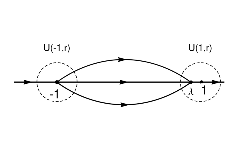
Figure 1: Regions and contours for $\Psi$

(a)ย ย  ฮจโ€‹(ฮถ;s)ฮจ๐œ๐‘ \Psi(\zeta;s) ($\Psi(\zeta)$, for short) is analytic in $\mathbb{C}\backslash\bigcup_{j=1}^{4}\Sigma_{j}$; see Fig.โ€„1 for the jump contours;

(b)ย ย  ฮจโ€‹(ฮถ)ฮจ๐œ\Psi(\zeta) satisfies the jump condition

$$\displaystyle\Psi_{+}(\zeta)=\Psi_{-}(\zeta)\left\{\begin{array}[]{ll}\left(\begin{array}[]{cc}1&\omega\\ 0&1\\ \end{array}\right),&\zeta\in{\Sigma}_{1},\\[11.38092pt] \left(\begin{array}[]{cc}1&0\\ e^{2\alpha\pi i}&1\\ \end{array}\right),&\zeta\in{\Sigma}_{2},\\[11.38092pt] \left(\begin{array}[]{cc}0&1\\ -1&0\\ \end{array}\right),&\zeta\in{\Sigma}_{3},\\[11.38092pt] \left(\begin{array}[]{cc}1&0\\ e^{-2\alpha\pi i}&1\\ \end{array}\right),&\zeta\in\Sigma_{4};\end{array}\right.$$ (2.13)

(c)ย ย  As $\zeta\rightarrow\infty$

ฮจโ€‹(ฮถ)=ฮถโˆ’14โ€‹ฯƒ3โ€‹M0โ€‹[I+ฯƒ^โ€‹(s)โ€‹(ฯƒ3โˆ’iโ€‹ฯƒ1)2โ€‹ฮถโˆ’(ฯƒ^โ€ฒโ€‹(s)+ฯƒ^2โ€‹(s))โ€‹ฯƒ22โ€‹ฮถ+Oโ€‹(ฮถโˆ’32)]โ€‹eโˆ’ฯ‘โ€‹ฯƒ3=[I+12โ€‹ฮถโ€‹(ฯƒ^โ€ฒโ€‹(s)+ฯƒ^2โ€‹(s)โˆ’2โ€‹iโ€‹ฯƒ^โ€‹(s)โˆ’(ฯƒ^โ€ฒโ€‹(s)+ฯƒ^2โ€‹(s)))+Oโ€‹(ฮถโˆ’2)]โ€‹ฮถโˆ’14โ€‹ฯƒ3โ€‹M0โ€‹eโˆ’ฯ‘โ€‹ฯƒ3,ฮจ๐œabsentsuperscript๐œ14subscript๐œŽ3subscript๐‘€0delimited-[]๐ผ^๐œŽ๐‘ subscript๐œŽ3๐‘–subscript๐œŽ12๐œsuperscript^๐œŽโ€ฒ๐‘ superscript^๐œŽ2๐‘ subscript๐œŽ22๐œ๐‘‚superscript๐œ32superscript๐‘’italic-ฯ‘subscript๐œŽ3missing-subexpressionabsentdelimited-[]๐ผ12๐œsuperscript^๐œŽโ€ฒ๐‘ superscript^๐œŽ2๐‘ 2๐‘–^๐œŽ๐‘ missing-subexpressionsuperscript^๐œŽโ€ฒ๐‘ superscript^๐œŽ2๐‘ ๐‘‚superscript๐œ2superscript๐œ14subscript๐œŽ3subscript๐‘€0superscript๐‘’italic-ฯ‘subscript๐œŽ3\begin{array}[]{rl}\Psi(\zeta)&=\zeta^{-\frac{1}{4}\sigma_{3}}M_{0}\left[I+\frac{\hat{\sigma}(s)(\sigma_{3}-i\sigma_{1})}{2\sqrt{\zeta}}-\frac{(\hat{\sigma}^{\prime}(s)+\hat{\sigma}^{2}(s))\sigma_{2}}{2\zeta}+O\left(\zeta^{-\frac{3}{2}}\right)\right]e^{-\vartheta\sigma_{3}}\\[8.5359pt] &=\left[I+\frac{1}{2\zeta}\left(\begin{array}[]{cc}\hat{\sigma}^{\prime}(s)+\hat{\sigma}^{2}(s)&-2i\hat{\sigma}(s)\\ &-(\hat{\sigma}^{\prime}(s)+\hat{\sigma}^{2}(s))\end{array}\right)+O\left(\zeta^{-2}\right)\right]\zeta^{-\frac{1}{4}\sigma_{3}}M_{0}e^{-\vartheta\sigma_{3}},\end{array} (2.14)

where $M_{0}=\frac{I+i\sigma_{1}}{\sqrt{2}}$, ฯ‘=ฯ‘โ€‹(ฮถ,s)=23โ€‹ฮถ3/2+sโ€‹ฮถ1/2italic-ฯ‘italic-ฯ‘๐œ๐‘ 23superscript๐œ32๐‘ superscript๐œ12\vartheta=\vartheta(\zeta,s)=\frac{2}{3}\zeta^{3/2}+s\zeta^{1/2}, and $\sigma_{j}$ are the Pauli matrices, namely,

$$\sigma_{1}=\left(\begin{array}[]{cc}0&1\\ 1&0\\ \end{array}\right),~{}~{}\sigma_{2}=\left(\begin{array}[]{cc}0&-i\\ i&0\\ \end{array}\right),~{}~{}\mbox{and}~{}\sigma_{3}=\left(\begin{array}[]{cc}1&0\\ 0&-1\\ \end{array}\right);$$

(d)ย ย  As $\zeta\rightarrow 0$, $\zeta\in\Omega_{j}$ for $j=1,2,3,4$,

$$\Psi(\zeta)=\Psi_{0}(\zeta)\zeta^{\alpha\sigma_{3}}E_{j}~{}~{}\mbox{if}~{}2\alpha\notin\mathbb{N}_{0},$$ (2.15)

or

$$\Psi(\zeta)=\Psi_{0}(\zeta)\zeta^{\alpha\sigma_{3}}\left(I+\frac{k}{2}(\ln\zeta+\pi)\sigma_{+}\right)E_{j}~{}~{}\mbox{if}~{}2\alpha\in\mathbb{N}_{0},$$ (2.16)

where $\sigma_{+}=\left(\begin{array}[]{cc}0&1\\ 0&0\\ \end{array}\right)$, $\Psi_{0}(\zeta)$ is analytic at $\zeta=0$, and $E_{j}$ are certain constant matrices; see [16, (3.21)].

PROPOSITION 1.

For $\alpha>-\frac{1}{2}$ and $\omega\in\mathbb{C}\setminus(-\infty,0)$, there exits a unique solution to the above Riemann-Hilbert problem for ฮจโ€‹(ฮถ;s)ฮจ๐œ๐‘ \Psi(\zeta;s).

Proof.

The existence of the solution $\Psi(\zeta)$ is obtained by proving a vanishing lemma; see [17] and [24] for a proof of the vanishing lemma. โˆŽ

Now we observe that the entries of $\Psi(\zeta)$ are closely related with equations (1.13) and (1.20) as follows:

PROPOSITION 2.

Let

ฯƒโ€‹(s)=iโ€‹limฮถโ†’โˆžฮถโ€‹(ฮจโ€‹(ฮถ;s)โ€‹eฯ‘โ€‹ฯƒ3โ€‹Iโˆ’iโ€‹ฯƒ12โ€‹ฮถ14โ€‹ฯƒ3)12+s24,๐œŽ๐‘ ๐‘–subscriptโ†’๐œ๐œsubscriptฮจ๐œ๐‘ superscript๐‘’italic-ฯ‘subscript๐œŽ3๐ผ๐‘–subscript๐œŽ12superscript๐œ14subscript๐œŽ312superscript๐‘ 24\sigma(s)=i\lim_{\zeta\rightarrow\infty}\zeta\left(\Psi(\zeta;s)e^{\vartheta\sigma_{3}}\frac{I-i\sigma_{1}}{\sqrt{2}}\zeta^{\frac{1}{4}\sigma_{3}}\right)_{12}+\frac{s^{2}}{4}, (2.17)

then ฯƒโ€‹(s)๐œŽ๐‘ \sigma(s) satisfies the Jimbo-Miwa-Okamoto $\sigma$-form of the Painlevรฉ II equation (1.13). Also,

uโ€‹(s)=โˆ’ฯƒโ€ฒโ€‹(s)๐‘ข๐‘ superscript๐œŽโ€ฒ๐‘ u(s)=-\sigma^{\prime}(s)

satisfies the Painlevรฉ XXXIV equation (1.20). Moreover, for $\alpha>-\frac{1}{2}$ and $\omega\in\mathbb{C}\setminus(-\infty,0)$, the scalar functions ฯƒโ€‹(s)๐œŽ๐‘ \sigma(s) and uโ€‹(s)๐‘ข๐‘ u(s) are analytic for sโˆˆโ„๐‘ โ„s\in\mathbb{R}.

Let ฮจ^โ€‹(ฮถ;s)=(10iโ€‹(ฯƒโ€‹(s)โˆ’s24)1)โ€‹ฮจโ€‹(ฮถ;s)^ฮจ๐œ๐‘ 10๐‘–๐œŽ๐‘ superscript๐‘ 241ฮจ๐œ๐‘ \widehat{\Psi}(\zeta;s)=\left(\begin{array}[]{cc}1&0\\ i(\sigma(s)-\frac{s^{2}}{4})&1\\ \end{array}\right)\Psi(\zeta;s), then ฮจ^โ€‹(ฮถ;s)^ฮจ๐œ๐‘ \widehat{\Psi}(\zeta;s) satisfies the following Lax pair system of differential equations

โˆ‚โˆ‚ฮถโ€‹ฮจ^โ€‹(ฮถ;s)=(uโ€ฒ2โ€‹ฮถiโˆ’iโ€‹uฮถโˆ’iโ€‹ฮถโˆ’iโ€‹(u+s)โˆ’iโ€‹(uโ€ฒ)2โˆ’(2โ€‹ฮฑ)24โ€‹uโ€‹ฮถโˆ’uโ€ฒ2โ€‹ฮถ)โ€‹ฮจ^โ€‹(ฮถ;s),๐œ^ฮจ๐œ๐‘ superscript๐‘ขโ€ฒ2๐œ๐‘–๐‘–๐‘ข๐œ๐‘–๐œ๐‘–๐‘ข๐‘ ๐‘–superscriptsuperscript๐‘ขโ€ฒ2superscript2๐›ผ24๐‘ข๐œsuperscript๐‘ขโ€ฒ2๐œ^ฮจ๐œ๐‘ \displaystyle\frac{\partial}{\partial\zeta}\widehat{\Psi}(\zeta;s)=\left(\begin{array}[]{cc}\frac{u^{\prime}}{2\zeta}&i-i\frac{u}{\zeta}\\ -i\zeta-i(u+s)-i\frac{(u^{\prime})^{2}-(2\alpha)^{2}}{4u\zeta}&-\frac{u^{\prime}}{2\zeta}\\ \end{array}\right)\widehat{\Psi}(\zeta;s),
โˆ‚โˆ‚sโ€‹ฮจ^โ€‹(ฮถ;s)=(0iโˆ’iโ€‹ฮถโˆ’2โ€‹iโ€‹(u+s2)0)โ€‹ฮจ^โ€‹(ฮถ;s);๐‘ ^ฮจ๐œ๐‘ 0๐‘–๐‘–๐œ2๐‘–๐‘ข๐‘ 20^ฮจ๐œ๐‘ \displaystyle\frac{\partial}{\partial s}\widehat{\Psi}(\zeta;s)=\left(\begin{array}[]{cc}0&i\\ -i\zeta-2i(u+\frac{s}{2})&0\\ \end{array}\right)\widehat{\Psi}(\zeta;s);

see [16, Lemma 3.2].

It is well known that the Painlevรฉ XXXIV equation (1.20) is related to the Painlevรฉ II equation

qโ€ฒโ€ฒ=sโ€‹q+2โ€‹q3โˆ’(2โ€‹ฮฑ+12)superscript๐‘žโ€ฒโ€ฒ๐‘ ๐‘ž2superscript๐‘ž32๐›ผ12q^{\prime\prime}=sq+2q^{3}-(2\alpha+\frac{1}{2}) (2.18)

by the formulas

uโ€‹(s)=213โ€‹Uโ€‹(โˆ’2โˆ’13โ€‹s),Uโ€‹(s)=qโ€ฒ+q2+s2;formulae-sequence๐‘ข๐‘ superscript213๐‘ˆsuperscript213๐‘ ๐‘ˆ๐‘ superscript๐‘žโ€ฒsuperscript๐‘ž2๐‘ 2u(s)=2^{\frac{1}{3}}U(-2^{-\frac{1}{3}}s),\quad U(s)=q^{\prime}+q^{2}+\frac{s}{2}; (2.19)

see [9, (5.0.2)(5.0.55)]. Moreover, the solution uโ€‹(s)๐‘ข๐‘ u(s) associated with the model RH problem, as stated in Proposition 2, is related to a family of special solutions to the second Painlevรฉ equation (2.18) corresponding to the Stokes multipliers {s1=โˆ’eโˆ’2โ€‹ฯ€โ€‹iโ€‹ฮฑ,s2=ฯ‰,s3=โˆ’e2โ€‹ฯ€โ€‹iโ€‹ฮฑ}formulae-sequencesubscript๐‘ 1superscript๐‘’2๐œ‹๐‘–๐›ผformulae-sequencesubscript๐‘ 2๐œ”subscript๐‘ 3superscript๐‘’2๐œ‹๐‘–๐›ผ\{s_{1}=-e^{-2\pi i\alpha},s_{2}=\omega,s_{3}=-e^{2\pi i\alpha}\}; cf. [9, 11.3], see also [16, 24] for the relation between the model RH problem for $\Psi$ and the RH problem for the second Painlevรฉ equation. Thus we may extract the asymptotics of uโ€‹(s)๐‘ข๐‘ u(s), knowing that of qโ€‹(s)๐‘ž๐‘ q(s).

It is also known that the solutions qโ€‹(s)๐‘ž๐‘ q(s) corresponding to the Stokes multipliers {s1=โˆ’eโˆ’2โ€‹ฯ€โ€‹iโ€‹ฮฑ,s2=ฯ‰,s3=โˆ’e2โ€‹ฯ€โ€‹iโ€‹ฮฑ}formulae-sequencesubscript๐‘ 1superscript๐‘’2๐œ‹๐‘–๐›ผformulae-sequencesubscript๐‘ 2๐œ”subscript๐‘ 3superscript๐‘’2๐œ‹๐‘–๐›ผ\{s_{1}=-e^{-2\pi i\alpha},s_{2}=\omega,s_{3}=-e^{2\pi i\alpha}\} is uniquely determined by the following asymptotic behavior

qโ€‹(s)=โˆ’s2โ€‹โˆ‘k=0nbkโ€‹(โˆ’s)32โ€‹k+Oโ€‹(sโˆ’32โ€‹nโˆ’1)+c+โ€‹(โˆ’s)โˆ’3โ€‹ฮฑโˆ’1โ€‹eโˆ’2โ€‹23โ€‹(โˆ’s)32โ€‹(1+Oโ€‹(sโˆ’14)),๐‘ž๐‘ ๐‘ 2superscriptsubscript๐‘˜0๐‘›subscript๐‘๐‘˜superscript๐‘ 32๐‘˜๐‘‚superscript๐‘ 32๐‘›1subscript๐‘superscript๐‘ 3๐›ผ1superscript๐‘’223superscript๐‘ 321๐‘‚superscript๐‘ 14q(s)=\sqrt{\frac{-s}{2}}\sum_{k=0}^{n}b_{k}(-s)^{\frac{3}{2}k}+O\left(s^{-\frac{3}{2}n-1}\right)+c_{+}(-s)^{-3\alpha-1}e^{-\frac{2\sqrt{2}}{3}(-s)^{\frac{3}{2}}}\left(1+O\left(s^{-\frac{1}{4}}\right)\right), (2.20)

as arg(โˆ’s)โˆˆ(โˆ’ฯ€3,ฯ€3]arg๐‘ ๐œ‹3๐œ‹3\mathop{\rm arg}\nolimits(-s)\in(-\frac{\pi}{3},\frac{\pi}{3}] and sโ†’โˆžโ†’๐‘ s\to\infty, [9, (11.5.56)]. The first few coefficients are

$$b_{0}=1,\quad b_{1}=\frac{\alpha}{\sqrt{2}},\quad b_{2}=-\frac{1+6\alpha^{2}}{8},$$

and

$$c_{+}=\frac{e^{2\pi i\alpha}-\omega}{\pi}2^{-5\alpha-3}\Gamma(2\alpha+1);$$

see [9, (11.5.58) and (11.5.68)]. A combination of the asymptotics of qโ€‹(s)๐‘ž๐‘ q(s) and the relation (2.19) will then gives the asymptotic approximations of uโ€‹(s)๐‘ข๐‘ u(s) and ฯƒโ€‹(s)๐œŽ๐‘ \sigma(s) as sโ†’โˆžโ†’๐‘ s\to\infty and argsโˆˆ(โˆ’ฯ€3,ฯ€3]arg๐‘ ๐œ‹3๐œ‹3\mathop{\rm arg}\nolimits s\in(-\frac{\pi}{3},\frac{\pi}{3}], as stated in (1.17) and (1.21).

We also mention that, for $\alpha=0$ and $\omega=1$, the solution $q(x)$ determined by (2.20) or the Stokes multipliers {s1=โˆ’1,s2=1,s3=โˆ’1}formulae-sequencesubscript๐‘ 11formulae-sequencesubscript๐‘ 21subscript๐‘ 31\{s_{1}=-1,s_{2}=1,s_{3}=-1\} is the classical solution

$$q(x)=-2^{-1/3}\frac{{\rm Ai}^{\prime}(-2^{-1/3}x)}{{\rm Ai}(-2^{-1/3}x)};$$

cf. [9, (11.4.15)]. Thus by (2.19) the Painlevรฉ XXXIV function corresponding to the parameter $\alpha=0$ and $\omega=1$ is trivial, that is, $u(x)=0$; see also [24, Lemma 3].

The asymptotics of qโ€‹(s)๐‘ž๐‘ q(s) as sโ†’+โˆžโ†’๐‘ s\to+\infty can be found in, e.g. [9, Chapter 10]. However, the leading asymptotics of qโ€‹(s)๐‘ž๐‘ q(s) is canceled out when we substitute it into (2.19). Therefore, the leading term alone is not enough to derive the asymptotics of uโ€‹(s)๐‘ข๐‘ u(s); see also the discussion in [16, 17]. We will derive the asymptotics of uโ€‹(s)๐‘ข๐‘ u(s) and ฯƒโ€‹(s)๐œŽ๐‘ \sigma(s) as sโ†’โˆ’โˆžโ†’๐‘ s\to-\infty by using the RH problem for $\Psi$. Details will be given in the Appendix.

3 Nonlinear steepest descend analysis of orthogonal polynomials

In this section, we start by presenting the RH problem $Y(z;\mu,n)$ for the orthogonal polynomials associated with the weight function (1.2). Then we show that the logarithmic derivative of the Hankel determinants can be expressed in terms of the solutions to this RH problem. For $n$ fixed, by relating the solution $Y(z;\mu,n)$ to the Lax pair for the Painlevรฉ IV equation, we show that the logarithmic derivative of the Hankel determinant satisfies the Jimbo-Miwa-Okamoto $\sigma$-form of the Painlevรฉ IV equation. Then we perform a nonlinear steepest descent analysis of the RH problem for $Y$ via the Deift-Zhou method [8, 6, 7] .

3.1 Riemann-Hilbert problem for orthogonal polynomials

The RH problem for the orthogonal polynomials with respect to (1.2) is as follows.

(Y1)ย ย  Yโ€‹(z)๐‘Œ๐‘งY(z) is analytic in $\mathbb{C}\backslash\mathbb{R}$;

(Y2)ย ย  Yโ€‹(z)๐‘Œ๐‘งY(z) satisfies the jump condition

$$Y_{+}(x)=Y_{-}(x)\left(\begin{array}[]{cc}1&w(x)\\ 0&1\\ \end{array}\right),\qquad x\in\mathbb{R},$$ (3.1)

where $w(x)$ is defined in (1.2);

(Y3)ย ย  The behavior of $Y(z)$ at infinity is

$$Y(z)=\left(I+\frac{Y_{1}}{z}+\frac{Y_{2}}{z^{2}}+O\left(\frac{1}{z^{3}}\right)\right)\left(\begin{array}[]{cc}z^{n}&0\\ 0&z^{-n}\\ \end{array}\right),\quad\quad z\rightarrow\infty;$$ (3.2)

(Y4)ย ย  The behavior of $Y(z)$ at $\mu$ is

$$Y(z)=\left\{\begin{array}[]{ll}O\left(\begin{array}[]{cc}1&|z-\mu|^{2\alpha}\\ 1&|z-\mu|^{2\alpha}\\ \end{array}\right),&z\rightarrow\mu,\quad\alpha<0,\\[11.38092pt] O\left(\begin{array}[]{cc}1&\log|z-\mu|\\ 1&\log|z-\mu|\\ \end{array}\right),&z\rightarrow\mu,\quad\alpha=0,\\[11.38092pt] O\left(\begin{array}[]{cc}1&1\\ 1&1\\ \end{array}\right),&z\rightarrow\mu,\quad\alpha>0.\end{array}\right.$$ (3.3)

For $\alpha>-\frac{1}{2}$ and $\omega\geq 0$, the system of orthogonal polynomials with respect to (1.2) are well defined. It follows from the Sochocki-Plemelj formula and Liouvilleโ€™s theorem that the unique solution of the RH problem for $Y$ is given by

$$Y(z)=\left(\begin{array}[]{cc}\pi_{n}(z)&\frac{1}{2\pi i}\int_{\mathbb{R}}\frac{\pi_{n}(x)w(x)}{x-z}dx\\ -2\pi i\gamma_{n-1}^{2}\;\pi_{n-1}(z)&-\gamma_{n-1}^{2}\;\int_{\mathbb{R}}\frac{\pi_{n-1}(x)w(x)}{x-z}dx\end{array}\right).$$ (3.4)

where $\pi_{n}(z)$ is the monic orthogonal polynomial with respect to the weight $w(x)$ defined in (1.2); see [10]. For general $\omega\in\mathbb{C}\setminus(-\infty,0)$, we will prove later that for $n$ large enough, the RH problem for $Y$ can be solved and thus the polynomials orthogonal with respect to (1.2) exist for large $n$.

Now we introduce

$$\Phi(z,\mu)=Y(z+\mu)e^{-\left(\frac{z^{2}}{2}+\mu z\right)\sigma_{3}}z^{\alpha\sigma_{3}},$$ (3.5)

then $\Phi(z,\mu)$ satisfies constant jumps on the real axis and has a regular singularity at $z=0$ and an irregular singularity at infinity, with

$$\Phi(z,\mu)=\left(I+\frac{Y_{1}+n\mu\sigma_{3}}{z}+O\left(\frac{1}{z^{2}}\right)\right)e^{-\left(\frac{z^{2}}{2}+\mu z\right)\sigma_{3}}z^{(n+\alpha)\sigma_{3}},\quad\quad z\rightarrow\infty.$$ (3.6)

Thus, it is related to the Garnier-Jimbo-Miwa Lax pair $\Phi_{\mathrm{PIV}}$ for the Painlevรฉ IV equation with the parameters $\theta_{\infty}=-(\alpha+n)$ and $\theta_{0}=\alpha$ by

$$\Phi(z,\mu)=\Phi_{\mathrm{PIV}}(e^{\frac{1}{2}\pi i}z,e^{\frac{1}{2}\pi i}\mu)e^{-\frac{\pi}{2}i(\alpha+n)\sigma_{3}};$$ (3.7)

see [9, Theorem 5.2,Proposition 5.4] and [18, Eq.(C.30)-Eq.(C.34)]. From this relation, we get the $\sigma$-form of the Painlevรฉ IV equation [18, Eq.(C.30)-Eq.(C.37)].

PROPOSITION 3.

Let

$$\sigma_{\mathrm{IV}}(\mu)=2\lim_{z\to\infty}z(Y(z)z^{-n\sigma_{3}}-I)_{11},$$ (3.8)

then $\sigma_{\mathrm{IV}}$ satisfies the Jimbo-Miwa-Okamoto $\sigma$-form of the Painlevรฉ IV equation

$$(\sigma_{\mathrm{IV}}^{\prime\prime})^{2}=4(\mu\sigma_{\mathrm{IV}}^{\prime}-\sigma_{\mathrm{IV}})^{2}-4\sigma_{\mathrm{IV}}^{\prime}(\sigma_{\mathrm{IV}}^{\prime}-4\alpha)(\sigma_{\mathrm{IV}}^{\prime}+2n).$$ (3.9)

At the end of this section, we state and prove a differential identity for the Hankel determinant associated with the weight $w(x)$ in (1.2). The identity serves as the start point of our asymptotic study of the Hankel determinant. We also show that the logarithmic derivative of the Hankel determinant satisfies the Jimbo-Miwa-Okamoto $\sigma$-form of the Painlevรฉ IV equation, as was first obtained in [12].

LEMMA 1.

Let $H_{n}$ be the Hankel determinant associated with $w(x;\mu)$ in (1.1), then

$$\frac{d}{d\mu}\ln H_{n}=2\lim_{z\to\infty}z(Y(z)z^{-n\sigma_{3}}-I)_{11},$$ (3.10)

and $\sigma_{\mathrm{IV}}(\mu)=\frac{d}{d\mu}\ln H_{n}$ satisfies the Jimbo-Miwa-Okamoto $\sigma$-form of the Painlevรฉ IV equation

$$(\sigma_{\mathrm{IV}}^{\prime\prime})^{2}=4(\mu\sigma_{\mathrm{IV}}^{\prime}-\sigma_{\mathrm{IV}})^{2}-4\sigma_{\mathrm{IV}}^{\prime}(\sigma_{\mathrm{IV}}^{\prime}-4\alpha)(\sigma_{\mathrm{IV}}^{\prime}+2n).$$ (3.11)
Proof.

By (1.6) and taking logarithmic derivative with respect to $\mu$, we have

$$\frac{d}{d\mu}\ln H_{n}=-2\sum_{k=0}^{n-1}\gamma_{k}^{-1}\frac{d}{d\mu}\gamma_{k},$$ (3.12)

where

$$\gamma_{k}^{-2}=\int_{\mathbb{R}}\pi_{k}(x)^{2}w(x)dx=\int_{\mathbb{R}}(\pi_{k}(x+\mu))^{2}w(x+\mu)dx.$$ (3.13)

Taking derivative with respect to $\mu$ on both sides of (3.13) and using the orthogonality and the definition of the weight (1.2), we get

$$\gamma_{k}^{-1}\frac{d}{d\mu}\gamma_{k}=\gamma_{k}^{2}\int_{\mathbb{R}}(x+\mu)\pi_{k}(x+\mu)^{2}w(x+\mu)dx=\gamma_{k}^{2}\int_{\mathbb{R}}x\pi_{k}(x)^{2}w(x)dx.$$ (3.14)

It follows from (3.12), (3.14) and the Christoffel-Darboux formula that

$$\frac{d}{d\mu}\ln H_{n}=-2\gamma_{n-1}^{2}\int_{\mathbb{R}}x\left(\frac{d}{dx}\pi_{n}(x)\pi_{n-1}(x)-\pi_{n}(x)\frac{d}{dx}\pi_{n-1}(x)\right)w(x)dx.$$ (3.15)

Write $\pi_{n}(x)=x^{n}+p_{n}x^{n-1}+\cdots$, we have the following decomposition into the orthogonal system $\{\pi_{k}\}_{k=0}^{n}$,

$$x\frac{d}{dx}\pi_{n}(x)=n\pi_{n}-p_{n}\pi_{n-1}+\cdots$$ (3.16)

By using the orthogonality, we have $\frac{d}{d\mu}\ln H_{n}=2p_{n}$. Then (3.10) follows from (3.4), and the fulfilment of (3.11) follows from Proposition 3. โˆŽ

3.2 The transformations $Y\rightarrow T\to S$

From this section on, we take ฮผ:=ฮผn=2โ€‹n+s2โ€‹n1/6assign๐œ‡subscript๐œ‡๐‘›2๐‘›๐‘ 2superscript๐‘›16\mu:=\mu_{n}=\sqrt{2n}+\frac{s}{\sqrt{2}n^{1/6}} in the weight function (1.2). We introduce the transformation

$$T(z)=(2n)^{-\frac{1}{2}(n+\alpha)\sigma_{3}}e^{-\frac{1}{2}nl\sigma_{3}}Y(\sqrt{2n}z)e^{n\left(\frac{1}{2}l-g(z)\right)\sigma_{3}}(2n)^{\frac{\alpha}{2}\sigma_{3}},\quad z\in\mathbb{C}\backslash\mathbb{R},$$ (3.17)

where the $g$-function

$$g(z)=\int_{-1}^{1}\ln(z-x)\varphi(x)dx,\quad\varphi(x)=\frac{2}{\pi}\sqrt{1-x^{2}},\quad z\in\mathbb{C}\setminus(-\infty,1],$$ (3.18)

and $l=\-1-2\ln 2$, with the logarithm taking the branch $\mathop{\rm arg}\nolimits(z-x)\in(-\pi,\pi)$. We also introduce the $\phi$-function

$$\phi(z)=2\int_{1}^{z}\sqrt{x^{2}-1}dx=z\sqrt{z^{2}-1}-\ln\left(z+\sqrt{z^{2}-1}\right),\quad z\in\mathbb{C}\setminus(-\infty,1],$$ (3.19)

where the branches are chosen such that $\sqrt{z^{2}-1}$ is analytic in $\mathbb{C}\setminus[-1,1]$, taking positive values on $(1,+\infty)$, $z+\sqrt{z^{2}-1}$ maps $\mathbb{C}\setminus[-1,1]$ onto the outside of the unit disk, with $z+\sqrt{z^{2}-1}\sim 2z$ as $z\to\infty$, and the logarithm taking the principal branch. The $\phi$-function and $g$-function are related by the phase condition

$$2\left[g(z)+\phi(z)\right]-2z^{2}-l=0,\quad z\in\mathbb{C}\backslash(-\infty,1].$$ (3.20)

So defined, $T$ is normalized at infinity in the sense that $T(z)=I+O(1/z)$, and satisfies the jump condition

$$T_{+}(x)=T_{-}(x)\left\{\begin{array}[]{ll}\left(\begin{array}[]{cc}1&|x-\lambda|^{2\alpha}\theta(x-\lambda)e^{-2n\phi(x)}\\ 0&1\\ \end{array}\right),&x\in(1,+\infty),\\ &\\ \left(\begin{array}[]{cc}e^{2n\phi_{+}(x)}&|x-\lambda|^{2\alpha}\theta(x-\lambda)\\ 0&e^{2n\phi_{-}(x)}\\ \end{array}\right),&x\in(-1,1),\\ &\\ \left(\begin{array}[]{cc}1&|x-\lambda|^{2\alpha}e^{-2n\phi_{+}(x)}\\ 0&1\\ \end{array}\right),&x\in(-\infty,-1),\end{array}\right.$$ (3.21)

where ฮป=ฮผn2โ€‹n=1+s2โ€‹n2/3๐œ†subscript๐œ‡๐‘›2๐‘›1๐‘ 2superscript๐‘›23\lambda=\frac{\mu_{n}}{\sqrt{2n}}=1+\frac{s}{2n^{2/3}}, $\theta(x)=\omega$ for $x>0$ and $\theta(x)=1$ for $x<0$.

To remove the oscillation of the diagonal entries of the jump matrix on $(-1,1)$, we deform the interval $[-1,\lambda]$ into a lens-shaped region as illustrated in Fig.โ€„2, and introduce the following transformation

$$S(z)=\left\{\begin{array}[]{ll}T(z),&\mbox{for $z$ outside the lens,}\\ &\\ T(z)\left(\begin{array}[]{cc}1&0\\ -(\lambda-z)^{-2\alpha}e^{2n\phi(z)}&1\\ \end{array}\right),&\mbox{for $z$ in the upper lens,}\\ &\\ T(z)\left(\begin{array}[]{cc}1&0\\ (\lambda-z)^{-2\alpha}e^{2n\phi(z)}&1\\ \end{array}\right),&\mbox{for $z$ in the lower lens. }\end{array}\right.$$ (3.22)

It is easy to see that $S$ satisfies the jump conditions

Refer to caption
Figure 2: Regions and contours for $S$. $\Sigma_{S}$ consists of the bold oriented contours: $U(\pm 1.r)$ are disks of radius $r$, centered respectively at $\pm 1$.
$$S_{+}(z)=S_{-}(z)\left\{\begin{array}[]{ll}\left(\begin{array}[]{cc}1&\omega|x-\lambda|^{2\alpha}e^{-2n\phi(x)}\\ 0&1\\ \end{array}\right),&z=x\in(\max(\lambda,1),+\infty),\\[11.38092pt] \left(\begin{array}[]{cc}0&|x-\lambda|^{2\alpha}\\ -|x-\lambda|^{-2\alpha}&0\\ \end{array}\right),&z=x\in(-1,\min(\lambda,1)),\\[11.38092pt] \left(\begin{array}[]{cc}1&0\\ (\lambda-z)^{-2\alpha}e^{2n\phi(z)}&1\\ \end{array}\right),&z~{}\mbox{on lens},\\[11.38092pt] \left(\begin{array}[]{cc}1&|x-\lambda|^{2\alpha}e^{-2n\phi_{+}(x)}\\ 0&1\\ \end{array}\right),&z=x\in(-\infty,-1),\end{array}\right.$$ (3.23)

and

$$S_{+}(x)=S_{-}(x)\left\{\begin{array}[]{ll}\left(\begin{array}[]{cc}e^{2n\phi_{+}(x)}&\omega|x-\lambda|^{2\alpha}\\ 0&e^{2n\phi_{-}(x)}\\ \end{array}\right),&x\in(\lambda,1),~{}\mbox{if}~{}\lambda<1,\\[11.38092pt] \left(\begin{array}[]{cc}0&|x-\lambda|^{2\alpha}e^{-2n\phi(x)}\\ -|x-\lambda|^{-2\alpha}e^{2n\phi(x)}&0\\ \end{array}\right),&x\in(1,\lambda),~{}\mbox{if}~{}\lambda>1.\end{array}\right.$$ (3.24)

We note that for $n$ large, the jumps for $S$ is close to the identity matrix, except the one on $[-1,\lambda]$. Here both cases, namely $\lambda<1$ and $\lambda>1$, are possible.

3.3 Global Parametrix

The global parametrix solves the following approximating RH problem, with only the jump along $(-1,\lambda)$ remains:

(N1)ย ย  Nโ€‹(z)๐‘๐‘งN(z) is analytic in $\mathbb{C}\backslash[-1,\lambda]$;

(N2)

$$N_{+}(x)=N_{-}(x)\left(\begin{array}[]{cc}0&|x-\lambda|^{2\alpha}\\ -|x-\lambda|^{-2\alpha}&0\\ \end{array}\right),\quad x\in(-1,\lambda);$$ (3.25)

(N3)

$$N(z)=I+O(z^{-1}),\quad z\rightarrow\infty.$$ (3.26)

A solution of the RH problem can be constructed explicitly as

$$N(z)=d(\infty)^{\sigma_{3}}N_{0}(z)d(z)^{-\sigma_{3}},$$ (3.27)

where

$$N_{0}(z)=\left(\begin{array}[]{cc}\frac{\varsigma(z)+\varsigma^{-1}(z)}{2}&\frac{\varsigma(z)-\varsigma^{-1}(z)}{2i}\\ -\frac{\varsigma(z)-\varsigma^{-1}(z)}{2i}&\frac{\varsigma(z)+\varsigma^{-1}(z)}{2}\\ \end{array}\right),\quad\varsigma(z)=\left(\frac{z-\lambda}{z+1}\right)^{1/4},$$ (3.28)

where $\varsigma(z)$ is analytic in $\mathbb{C}\setminus[-1,\lambda]$, and $\varsigma(z)\sim 1$ as $z\to\infty$.

The Szegล‘ function $d(z)$ in (3.27) is analytic in $\mathbb{C}\setminus[-1,\lambda]$ and satisfies

$$d_{+}(x)d_{-}(x)=|x-\lambda|^{2\alpha},\quad x\in(-1,\lambda);$$

see [20]. Indeed, the Szegล‘ function can be written explicitly as

$$d(z)=(z-\lambda)^{\alpha}(\sqrt{z-\lambda}+\sqrt{z+1})^{-2\alpha}(1+\lambda)^{\alpha},\quad d(\infty)=\left(\frac{1+\lambda}{4}\right)^{\alpha},$$ (3.29)

where $\mathop{\rm arg}\nolimits(z+1)\in(-\pi,\pi)$, $\mathop{\rm arg}\nolimits(z-\lambda)\in(-\pi,\pi)$ and the logarithm takes the principal branch with the branch cut along $(-\infty,0)$.

3.4 Local parametrix at $z=-1$

The local parametrix at $z=-1$ satisfies the following RH problem.

(a)ย ย  P(โˆ’1)โ€‹(z)superscript๐‘ƒ1๐‘งP^{(-1)}(z) is analytic in $U(-1,r)\backslash\Sigma_{S}$; see Fig.โ€„2 for the contours;

(b)ย ย  P+(โˆ’1)โ€‹(z)=Pโˆ’(โˆ’1)โ€‹(z)โ€‹JSโ€‹(z),zโˆˆฮฃSโˆฉUโ€‹(โˆ’1,r)formulae-sequencesubscriptsuperscript๐‘ƒ1๐‘งsubscriptsuperscript๐‘ƒ1๐‘งsubscript๐ฝ๐‘†๐‘ง๐‘งsubscriptฮฃ๐‘†๐‘ˆ1๐‘ŸP^{(-1)}_{+}(z)=P^{(-1)}_{-}(z)J_{S}(z),~{}~{}z\in\Sigma_{S}\cap U(-1,r), where $J_{S}(z)$ are the jump matrices of $S(z)$ in (3.23);

(c)ย ย  P(โˆ’1)โ€‹(z)โ€‹Nโˆ’1โ€‹(z)=I+Oโ€‹(1/n)superscript๐‘ƒ1๐‘งsuperscript๐‘1๐‘ง๐ผ๐‘‚1๐‘›P^{(-1)}(z)N^{-1}(z)=I+O(1/n) for $z\in\partial U(-1,r)$.

Refer to caption
Figure 3: Regions and contours for $\Phi_{A}$

The local parametrix can be constructed as follows:

$$P^{(-1)}(z)=\sigma_{3}E_{-1}(z)\Phi_{A}\left(\frac{3}{2}n\phi(-z)^{2/3}\right)e^{n\phi(z)\sigma_{3}}\sigma_{3},$$ (3.30)

where $E_{-1}(z)$ is a certain matrix-valued function analytic in $U(-1,r)$, $\Phi_{A}$ is the Airy parametrix defined as

$$\Phi_{A}(z)=M\left\{\begin{array}[]{ll}\left(\begin{array}[]{cc}{\rm Ai}(z)&{\rm Ai}(e^{-\frac{2\pi i}{3}}z)\\ {\rm Ai}^{\prime}(z)&e^{-\frac{2\pi i}{3}}{\rm Ai}^{\prime}(e^{-\frac{2\pi i}{3}}z)\\ \end{array}\right)e^{-\frac{\pi i}{6}\sigma_{3}},&z\in\Omega_{1},\\[14.22636pt] \left(\begin{array}[]{cc}{\rm Ai}(z)&{\rm Ai}(e^{-\frac{2\pi i}{3}}z)\\ {\rm Ai}^{\prime}(z)&e^{-\frac{2\pi i}{3}}{\rm Ai}^{\prime}(e^{-\frac{2\pi i}{3}}z)\\ \end{array}\right)e^{-\frac{\pi i}{6}\sigma_{3}}\left(\begin{array}[]{cc}1&0\\ -1&1\\ \end{array}\right),&z\in\Omega_{2},\\[14.22636pt] \left(\begin{array}[]{cc}{\rm Ai}(z)&-e^{-\frac{2\pi i}{3}}{\rm Ai}(e^{\frac{2\pi i}{3}}z)\\ {\rm Ai}^{\prime}(z)&-{\rm Ai}^{\prime}(e^{\frac{2\pi i}{3}}z)\\ \end{array}\right)e^{-\frac{\pi i}{6}\sigma_{3}}\left(\begin{array}[]{cc}1&0\\ 1&1\\ \end{array}\right),&z\in\Omega_{3},\\[14.22636pt] \left(\begin{array}[]{cc}{\rm Ai}(z)&-e^{-\frac{2\pi i}{3}}{\rm Ai}(e^{\frac{2\pi i}{3}}z)\\ {\rm Ai}^{\prime}(z)&-{\rm Ai}^{\prime}(e^{\frac{2\pi i}{3}}z)\\ \end{array}\right)e^{-\frac{\pi i}{6}\sigma_{3}},&z\in\Omega_{4},\end{array}\right.$$ (3.31)

with the regions indicated in Fig. 3 and $M=\sqrt{2\pi}e^{\frac{1}{6}\pi i}\left(\begin{array}[]{cc}1&0\\ 0&-i\\ \end{array}\right)$; cf. [7, (7.9)] and [4, Ch.โ€„7.6]. The Airy parametrix $\Phi_{A}$ satisfies the asymptotic condition at infinity

$$\Phi_{A}(z)=z^{-\sigma_{3}/4}\left(I+O(z^{-3/2})\right)\frac{I+i\sigma_{1}}{\sqrt{2}}e^{-\frac{2}{3}z^{\frac{3}{2}\sigma_{3}}}.$$ (3.32)

To match $P^{-1}(z)$ with the global parametrix $N(z)$, we choose

$$E_{-1}(z)=\sigma_{3}N(z)\sigma_{3}\left(\frac{3}{2}n\phi(-z)^{2/3}\right)^{\sigma_{3}/4}\frac{I-i\sigma_{1}}{\sqrt{2}}.$$

3.5 Local parametrix at $z=\lambda$

We seek a local parametrix $P^{(1)}(z)$ near ฮป=ฮผn2โ€‹n=1+s2โ€‹n2/3๐œ†subscript๐œ‡๐‘›2๐‘›1๐‘ 2superscript๐‘›23\lambda=\frac{\mu_{n}}{\sqrt{2n}}=1+\frac{s}{2n^{2/3}}. The parametrix solves the following RH problem:

(a)ย ย  P(1)โ€‹(z)superscript๐‘ƒ1๐‘งP^{(1)}(z) is analytic in $U(1,r)\backslash\Sigma_{S}$; see Fig.โ€„2 for the contours;

(b)ย ย  On $\Sigma_{S}\cap U(1,r)$, $P^{(1)}(z)$ satisfies the same jump condition as $S(z)$,

$$P^{(1)}_{+}(z)=P^{(1)}_{-}(z)J_{S},~{}~{}z\in\Sigma_{S}\cap U(1,r);$$ (3.33)

(c)ย ย  P(1)โ€‹(z)superscript๐‘ƒ1๐‘งP^{(1)}(z) satisfies the following matching condition on $\partial U(1,r)$:

$$P^{(1)}(z)N^{-1}(z)=I+O\left(n^{-1/3}\right);$$ (3.34)

(d)ย ย  The behavior at $z=\lambda$ is the same as that of $S(z)$.

It is observed that $P^{(1)}(z)e^{-n\phi(z)\sigma_{3}}(z-\lambda)^{\alpha\sigma_{3}}$ solves a RH problem with the same constant jumps as the model RH problem (2.13). We take the conformal mapping

$$f(z)=\left(\frac{3}{2}\phi(z)\right)^{2/3}=2(z-1)+O\left((z-1)^{2}\right)$$ (3.35)

from a neighborhood of $z=1$ to that of the origin. Then for $r$ small enough, the local parametrix ${P}^{(1)}(z)$ can be constructed as follows

$$P^{(1)}(z)=E(z)\Psi\left(n^{2/3}(f(z)-f(\lambda));n^{2/3}f(\lambda)\right)e^{n\phi(z)\sigma_{3}}(z-\lambda)^{-\alpha\sigma_{3}},$$ (3.36)

where

$$E(z)=N(z)(z-\lambda)^{\alpha\sigma_{3}}\frac{1}{\sqrt{2}}(I-i\sigma_{1})\left[n^{2/3}(f(z)-f(\lambda))\right]^{\sigma_{3}/4}.$$ (3.37)

To verify the matching condition (3.34), in view of (2.14), we can write the exponent of (3.36) as

$\displaystyle F_{n}(z):=$ $\displaystyle n\phi(z)-\vartheta\left((n^{2/3}(f(z)-f(\lambda)),n^{2/3}f(\lambda)\right)$
$\displaystyle=$ $\displaystyle\frac{n}{4}f(\lambda)^{2}(f(z)-f(\lambda))^{-\frac{1}{2}}\left[1+O(\lambda-1)\right]$ (3.38)
$\displaystyle=$ nโˆ’13โ€‹s24โ€‹(fโ€‹(z)โˆ’fโ€‹(ฮป))โˆ’12+Oโ€‹(1n)superscript๐‘›13superscript๐‘ 24superscript๐‘“๐‘ง๐‘“๐œ†12๐‘‚1๐‘›\displaystyle n^{-\frac{1}{3}}\frac{s^{2}}{4}\left(f(z)-f(\lambda)\right)^{-\frac{1}{2}}+O\left(\frac{1}{n}\right)

for $|z-1|=r$ and $n\to\infty$. Now substituting it in (2.14) and (3.36), we have the matching condition (3.34).

3.6 The final transformation: $S\rightarrow R$

The final transformation is defined as

$$R(z)=\left\{\begin{array}[]{ll}S(z)N^{-1}(z),&z\in\mathbb{C}\backslash\left\{U(-1,r)\cup U(1,r)\cup\Sigma_{S}\right\},\\ S(z)\left\{P^{(-1)}(z)\right\}^{-1},&z\in U(-1,r)\backslash\Sigma_{S},\\ S(z)\left\{P^{(1)}(z)\right\}^{-1},&z\in U(1,r)\backslash\Sigma_{S}.\end{array}\right.$$ (3.39)

From the matching condition (3.34), we have

$$\|J_{R}(z)-I\|_{L^{2}\cap L^{\infty}(\Sigma_{R})}=O(n^{-1/3}).$$ (3.40)

Thus

$$R(z)=I+O(n^{-1/3}),$$ (3.41)

where the error bound is uniform for $z$ in whole complex plane.

4 Proof of the main theorems

The differential identity (3.10) provides an expression of the logarithmic derivative of the Hankel determinant, in terms of the large-$z$ behavior of $Y(z)$; see (3.2). From (3.4), one can also write the recurrence coefficients in (1.5) as

$$a_{n}=(Y_{1})_{11}+\frac{(Y_{2})_{12}}{(Y_{1})_{12}}\quad\mbox{and}\quad b^{2}_{n}=(Y_{1})_{12}(Y_{1})_{21},$$ (4.1)

where $Y_{1}$ and $Y_{2}$ are the coefficients in the large-$z$ expansion of $Y(z)$ in (3.2). In this section, by using the asymptotics of $Y$ obtained in Section 3, we proceed to derive the large-$n$ asymptotic behavior of the Hankel determinant, the recurrence coefficients and the correlation kernel.

Tracing back the sequence of transformations $Y\to T\to S\to R$, given in (3.17), (3.22) and (3.39), we have

$$Y(\sqrt{2n}z)=(2n)^{\frac{1}{2}(n+\alpha)\sigma_{3}}e^{\frac{1}{2}nl\sigma_{3}}R(z)N(z)e^{ng(z)\sigma_{3}-\frac{1}{2}nl\sigma_{3}}(2n)^{-\frac{\alpha}{2}\sigma_{3}}.$$ (4.2)

As $z\rightarrow\infty$,

$$e^{ng(z)\sigma_{3}}z^{-n\sigma_{3}}=I+\frac{G_{1}}{z}+\frac{G_{2}}{z^{2}}+O\left(\frac{1}{z^{3}}\right),$$ (4.3)

where the matrix-valued coefficients $G_{1}=0$ and $G_{2}=\left\{-\frac{n}{2}\int_{-1}^{1}x^{2}\varphi(x)dx\right\}\sigma_{3}$. Denoting

$$N(z)=I+\frac{N_{1}}{z}+\frac{N_{2}}{z^{2}}+O\left(\frac{1}{z^{3}}\right)~{}~{}\mbox{as}~{}z\to\infty$$ (4.4)

and

$$R(z)=I+\frac{R_{1}}{z}+\frac{R_{2}}{z^{2}}+O\left(\frac{1}{z^{3}}\right)~{}~{}\mbox{as}~{}z\to\infty,$$ (4.5)

and substituting (4.4) and (4.5) in (4.2), we have

$$Y_{1}=(2n)^{\frac{\alpha}{2}\sigma_{3}}\sqrt{2n}e^{\frac{1}{2}nl\sigma_{3}}(R_{1}+N_{1})e^{-\frac{1}{2}nl\sigma_{3}}(2n)^{-\frac{\alpha}{2}\sigma_{3}},$$ (4.6)

and

$$Y_{2}=2n(2n)^{\frac{\alpha}{2}\sigma_{3}}e^{\frac{1}{2}nl\sigma_{3}}(R_{2}+G_{2}+N_{2}+R_{1}N_{1})e^{-\frac{1}{2}nl\sigma_{3}}(2n)^{-\frac{\alpha}{2}\sigma_{3}}.$$ (4.7)

To evaluate $N_{1}$ and $N_{2}$, we expand the Szegล‘ function (3.29) at infinity,

$\displaystyle d(z)=$ $\displaystyle\left(\frac{1+\lambda}{4}\right)^{\alpha}\left\{1-\frac{\alpha(\lambda+1)}{2}\frac{1}{z}\right.$
$\displaystyle\left.+\frac{4\alpha(2\alpha-1)+4\alpha(2\alpha-3)(\lambda-1)+\alpha(2\alpha-5)(\lambda-1)^{2}}{16z^{2}}+O\left(\frac{1}{z^{3}}\right)\right\}.$ (4.8)

We also expand $N_{0}(z)$ in (3.28) at infinity,

$$N_{0}(z)=I+\frac{N_{1}^{0}}{z}+\frac{N_{2}^{0}}{z^{2}}+O\left(\frac{1}{z^{3}}\right),$$ (4.9)

where

$$N_{1}^{0}=-\frac{1}{4}(1+\lambda)\sigma_{2},\ \ \ N_{2}^{0}=\frac{1-\lambda^{2}}{8}\sigma_{2}+\frac{(1+\lambda)^{2}}{32}I;$$ (4.10)

see [24]. Substituting (4)-(4.10) in (3.27) gives (4.4), with

$$N_{1}=\left(\frac{1+\lambda}{4}\right)^{\alpha\sigma_{3}}\left(-\frac{(1+\lambda)\sigma_{2}}{4}+\frac{\alpha(1+\lambda)\sigma_{3}}{2}\right)\left(\frac{1+\lambda}{4}\right)^{-\alpha\sigma_{3}},$$ (4.11)

and

$\displaystyle N_{2}=$ $\displaystyle\left(\frac{1+\lambda}{4}\right)^{\alpha\sigma_{3}}\left\{-\frac{i\alpha(1+\lambda)^{2}\sigma_{1}}{8}+\frac{(1-\lambda^{2})\sigma_{2}}{8}+\frac{(1+\lambda)^{2}I}{32}\right.$
$\displaystyle\left.+\frac{2\alpha^{2}(\lambda+1)^{2}I+(4\alpha+12\alpha(\lambda-1)+5\alpha(\lambda-1)^{2})\sigma_{3}}{16}\right\}\left(\frac{1+\lambda}{4}\right)^{-\alpha\sigma_{3}}.$ (4.12)

A combination of (2.14), (3.36) and (3.37) yields the following more precise description of the jump for $R(z)$ on $\partial U(1,r)$:

$\displaystyle J_{R}(z)=$ Nโ€‹(z)โ€‹(zโˆ’ฮป)ฮฑโ€‹ฯƒ3โ€‹(I+ฯƒ^โ€‹(s)โ€‹(ฯƒ3โˆ’iโ€‹ฯƒ1)2โ€‹n1/3โ€‹(fโ€‹(z)โˆ’fโ€‹(ฮป))1/2โˆ’(ฯƒ^โ€‹(s)2+ฯƒ^โ€ฒโ€‹(s))โ€‹ฯƒ22โ€‹n2/3โ€‹(fโ€‹(z)โˆ’fโ€‹(ฮป))+Oโ€‹(1n))๐‘๐‘งsuperscript๐‘ง๐œ†๐›ผsubscript๐œŽ3๐ผ^๐œŽ๐‘ subscript๐œŽ3๐‘–subscript๐œŽ12superscript๐‘›13superscript๐‘“๐‘ง๐‘“๐œ†12^๐œŽsuperscript๐‘ 2superscript^๐œŽโ€ฒ๐‘ subscript๐œŽ22superscript๐‘›23๐‘“๐‘ง๐‘“๐œ†๐‘‚1๐‘›\displaystyle N(z)(z-\lambda)^{\alpha\sigma_{3}}\left(I+\frac{\hat{\sigma}(s)(\sigma_{3}-i\sigma_{1})}{2n^{1/3}(f(z)-f(\lambda))^{1/2}}-\frac{(\hat{\sigma}(s)^{2}+\hat{\sigma}^{\prime}(s))\sigma_{2}}{2n^{2/3}(f(z)-f(\lambda))}+O\left(\frac{1}{n}\right)\right)
$\displaystyle\times e^{F_{n}(z)\sigma_{3}}(z-\lambda)^{-\alpha\sigma_{3}}N^{-1}(z),$ (4.13)

where $F_{n}(z)$ is defined in (3.5). In deriving (4), use has been made of the fact that n2/3โ€‹fโ€‹(ฮป)=s+Oโ€‹(nโˆ’2/3)superscript๐‘›23๐‘“๐œ†๐‘ ๐‘‚superscript๐‘›23n^{2/3}f(\lambda)=s+O(n^{-2/3}). From the approximation of $F_{n}$ in (3.5), we further have

$\displaystyle J_{R}(z)=$ $\displaystyle N(z)(z-\lambda)^{\alpha\sigma_{3}}\left\{I+\frac{(F_{1}+\varphi_{1})\sigma_{3}-i\varphi_{1}\sigma_{1}}{n^{1/3}}\right.$
$\displaystyle\left.+\frac{r_{4}(z,\lambda)I-r_{3}(z,\lambda)\sigma_{2}}{n^{2/3}}+O\left(\frac{1}{n}\right)\right\}(z-\lambda)^{-\alpha\sigma_{3}}N^{-1}(z),$ (4.14)

where

F1โ€‹(z,ฮป,n)=s24โ€‹(fโ€‹(z)โˆ’fโ€‹(ฮป))1/2,subscript๐น1๐‘ง๐œ†๐‘›superscript๐‘ 24superscript๐‘“๐‘ง๐‘“๐œ†12\displaystyle F_{1}(z,\lambda,n)=\frac{s^{2}}{4(f(z)-f(\lambda))^{1/2}}, (4.15)
ฯ†1โ€‹(z,ฮป)=ฯƒ^โ€‹(s)2โ€‹(fโ€‹(z)โˆ’fโ€‹(ฮป))1/2,ฯ†2โ€‹(z,ฮป)=โˆ’ฯƒ^โ€‹(s)2+ฯƒ^โ€ฒโ€‹(s)2โ€‹(fโ€‹(z)โˆ’fโ€‹(ฮป)),formulae-sequencesubscript๐œ‘1๐‘ง๐œ†^๐œŽ๐‘ 2superscript๐‘“๐‘ง๐‘“๐œ†12subscript๐œ‘2๐‘ง๐œ†^๐œŽsuperscript๐‘ 2superscript^๐œŽโ€ฒ๐‘ 2๐‘“๐‘ง๐‘“๐œ†\displaystyle\varphi_{1}(z,\lambda)=\frac{\hat{\sigma}(s)}{2(f(z)-f(\lambda))^{1/2}},\quad\varphi_{2}(z,\lambda)=-\frac{\hat{\sigma}(s)^{2}+\hat{\sigma}^{\prime}(s)}{2(f(z)-f(\lambda))}, (4.16)
$$\displaystyle r_{3}(z,\lambda)=F_{1}\varphi_{1}-\varphi_{2},\quad\mbox{and}\quad r_{4}(z,\lambda)=F_{1}\varphi_{1}+\frac{F_{1}^{2}}{2}.$$ (4.17)

Alternatively, $N_{0}(z)$ in (3.28) can be written as

$$N_{0}(z)=\frac{I-i\sigma_{1}}{\sqrt{2}}\varsigma(z)^{-\sigma_{3}}\frac{I+i\sigma_{1}}{\sqrt{2}}.$$

Accordingly, for $|z-1|=r$ we have

$$J_{R}(z)=d(\infty)^{\sigma_{3}}\frac{I-i\sigma_{1}}{\sqrt{2}}\left(I+\frac{\Delta_{1}(z)}{n^{1/3}}+\frac{\Delta_{2}(z)}{n^{2/3}}+O\left(\frac{1}{n}\right)\right)\frac{I+i\sigma_{1}}{\sqrt{2}}d(\infty)^{-\sigma_{3}},$$ (4.18)

where

$\displaystyle\Delta_{1}(z)$ $\displaystyle=\varsigma(z)^{-\sigma_{3}}\frac{I+i\sigma_{1}}{\sqrt{2}}d(z)^{-\sigma_{3}}(z-\lambda)^{\alpha\sigma_{3}}\left[(F_{1}+\varphi_{1})\sigma_{3}-i\varphi_{1}\sigma_{1}\right]$
$\displaystyle\quad\times(z-\lambda)^{-\alpha\sigma_{3}}d(z)^{\sigma_{3}}\frac{I-i\sigma_{1}}{\sqrt{2}}\varsigma(z)^{\sigma_{3}}$
$\displaystyle=\varsigma(z)^{-\sigma_{3}}\frac{I+i\sigma_{1}}{\sqrt{2}}\left[(F_{1}+\varphi_{1})\sigma_{3}-i\varphi_{1}\eta^{\sigma_{3}}\sigma_{1}\eta^{-\sigma_{3}}\right]\frac{I-i\sigma_{1}}{\sqrt{2}}\varsigma(z)^{\sigma_{3}}$
$\displaystyle=(F_{1}+\varphi_{1})\varsigma(z)^{-\sigma_{3}}\sigma_{2}\varsigma(z)^{\sigma_{3}}-i\varphi_{1}\varsigma(z)^{-\sigma_{3}}\frac{I+i\sigma_{1}}{\sqrt{2}}\eta^{\sigma_{3}}\sigma_{1}\eta^{-\sigma_{3}}\frac{I-i\sigma_{1}}{\sqrt{2}}\varsigma(z)^{\sigma_{3}}$
$\displaystyle=r_{1}(z,t)\sigma_{+}+r_{2}(z,t)\sigma_{-}-i\varphi_{1}\left(\frac{i\eta^{-2}-i\eta^{2}}{2}\sigma_{3}+\frac{\eta^{2}+\eta^{-2}-2}{2}\varsigma(z)^{-\sigma_{3}}\sigma_{1}\varsigma(z)^{\sigma_{3}}\right)$

and

$\displaystyle\Delta_{2}(z)$ $\displaystyle=\varsigma(z)^{-\sigma_{3}}\frac{I+i\sigma_{1}}{\sqrt{2}}d(z)^{-\sigma_{3}}(z-\lambda)^{\alpha\sigma_{3}}\left[r_{4}(z,t)I-r_{3}(z,t)\sigma_{2}\right]$
$\displaystyle\times(z-\lambda)^{-\alpha\sigma_{3}}d(z)^{\sigma_{3}}\frac{I-i\sigma_{1}}{\sqrt{2}}\varsigma(z)^{\sigma_{3}}$
$\displaystyle=\varsigma(z)^{-\sigma_{3}}\frac{I+i\sigma_{1}}{\sqrt{2}}\left[r_{4}(z,\lambda)I-r_{3}(z,\lambda)\eta^{\sigma_{3}}\sigma_{2}\eta^{-\sigma_{3}}\right]\frac{I-i\sigma_{1}}{\sqrt{2}}\varsigma(z)^{\sigma_{3}}$
$\displaystyle=r_{4}(z,\lambda)I-r_{3}(z,\lambda)\varsigma(z)^{-\sigma_{3}}\frac{I+i\sigma_{1}}{\sqrt{2}}\eta^{\sigma_{3}}\sigma_{2}\eta^{-\sigma_{3}}\frac{I-i\sigma_{1}}{\sqrt{2}}\varsigma(z)^{\sigma_{3}}$
$\displaystyle=r_{3}(z,\lambda)\sigma_{3}+r_{4}(z,\lambda)I+\frac{\eta^{2}+\eta^{-2}-2}{2}r_{3}(z,\lambda)\sigma_{3}$
$\displaystyle\quad+\frac{i\eta^{2}-i\eta^{-2}}{2}r_{3}(z,\lambda)\varsigma(z)^{-\sigma_{3}}\sigma_{1}\varsigma(z)^{\sigma_{3}},$

with

$$\displaystyle r_{1}(z,\lambda)=-\varsigma^{-2}(z)(F_{1}+2\varphi_{1})i,\quad r_{2}(z,\lambda)=\varsigma^{2}(z)F_{1}i,\quad\eta(z)=\frac{(z-\lambda)^{\alpha}}{d(z)}.$$ (4.19)

By (3.29), we have

$$\eta=1+2\alpha\sqrt{\frac{z-\lambda}{1+\lambda}}+2\alpha^{2}\frac{z-\lambda}{1+\lambda}+O((z-\lambda)^{3/2}),\quad z\rightarrow\lambda,$$ (4.20)

and hence

$$\eta^{2}+\eta^{-2}-2=O(z-\lambda),\quad\eta^{2}-\eta^{-2}=8\alpha\sqrt{\frac{z-\lambda}{1+\lambda}}+O(z-\lambda).$$ (4.21)

Thus

$$R(z)=d(\infty)^{\sigma_{3}}\frac{I-i\sigma_{1}}{\sqrt{2}}\left(I+\frac{R^{(1)}(z)}{n^{1/3}}+\frac{R^{(2)}(z)}{n^{2/3}}+O\left(\frac{1}{n}\right)\right)\frac{I+i\sigma_{1}}{\sqrt{2}}d(\infty)^{-\sigma_{3}},$$ (4.22)

where $R^{(1)}$ and $R^{(2)}$ satisfy the scalar RH problems

$$R^{(1)}_{+}(z)-R^{(1)}_{-}(z)=\Delta_{1}(z),~{}~{}R^{(2)}_{+}(z)-R^{(2)}_{-}(z)=\Delta_{2}(z)+R^{(1)}_{-}(z)\Delta_{1}(z).$$ (4.23)

From (4.15) and (4.19), we know that $r_{1}(z,t)$, $r_{3}(z,t)$ and $r_{4}(z,t)$ have a simple pole at $z=\lambda$ and $r_{2}(z,t)$ is analytic at $z=\lambda$. By Cauchyโ€™s theorem, we get

R(1)โ€‹(z)={k1โ€‹(s)zโˆ’ฮปโ€‹ฯƒ+โˆ’ฮ”1โ€‹(z),zโˆˆUโ€‹(1,r),k1โ€‹(s)zโˆ’ฮปโ€‹ฯƒ+,zโˆ‰Uโ€‹(1,r)ยฏ,superscript๐‘…1๐‘งcasessubscript๐‘˜1๐‘ ๐‘ง๐œ†subscript๐œŽsubscriptฮ”1๐‘ง๐‘ง๐‘ˆ1๐‘Ÿsubscript๐‘˜1๐‘ ๐‘ง๐œ†subscript๐œŽ๐‘งยฏ๐‘ˆ1๐‘ŸR^{(1)}(z)=\left\{\begin{array}[]{ll}\frac{k_{1}(s)}{z-\lambda}\sigma_{+}-\Delta_{1}(z),&z\in U(1,r),\\[8.5359pt] \frac{k_{1}(s)}{z-\lambda}\sigma_{+},&z\not\in\overline{U(1,r)},\end{array}\right. (4.24)

and

R(2)โ€‹(z)=k3โ€‹(t)โ€‹ฯƒ3+k4โ€‹(s)โ€‹Iโˆ’k1โ€‹(s)โ€‹k2โ€‹(s)โ€‹ฯƒโˆ’โ€‹ฯƒ++k5โ€‹(s)โ€‹ฯƒ+zโˆ’ฮป,zโˆ‰Uโ€‹(1,r)ยฏ.formulae-sequencesuperscript๐‘…2๐‘งsubscript๐‘˜3๐‘กsubscript๐œŽ3subscript๐‘˜4๐‘ ๐ผsubscript๐‘˜1๐‘ subscript๐‘˜2๐‘ subscript๐œŽsubscript๐œŽsubscript๐‘˜5๐‘ subscript๐œŽ๐‘ง๐œ†๐‘งยฏ๐‘ˆ1๐‘ŸR^{(2)}(z)=\frac{k_{3}(t)\sigma_{3}+k_{4}(s)I-k_{1}(s)k_{2}(s)\sigma_{-}\sigma_{+}+k_{5}(s)\sigma_{+}}{z-\lambda},\ \ z\not\in\overline{U(1,r)}. (4.25)

where kjโ€‹(s)=Resz=ฮปโ€‹rjโ€‹(z,ฮป)subscript๐‘˜๐‘—๐‘ subscriptRes๐‘ง๐œ†subscript๐‘Ÿ๐‘—๐‘ง๐œ†k_{j}(s)=\mathrm{Res}_{z=\lambda}r_{j}(z,\lambda) for $j=1,3,4$, k2โ€‹(s)=limzโ†’ฮปr2โ€‹(z,ฮป)subscript๐‘˜2๐‘ subscriptโ†’๐‘ง๐œ†subscript๐‘Ÿ2๐‘ง๐œ†k_{2}(s)=\lim_{z\rightarrow\lambda}r_{2}(z,\lambda) and k5โ€‹(s)subscript๐‘˜5๐‘ k_{5}(s) arises from the residue of the term $\eta$ in $\Delta_{2}(z)$ and $R^{(1)}_{-}(z)\Delta_{1}(z)$. After some careful calculations, we get from (4.19) and (4.15)

k1โ€‹(s)=โˆ’iโ€‹(ฯƒ^โ€‹(s)+s24)+Oโ€‹(nโˆ’2/3)k2โ€‹(s)=iโ€‹s28+Oโ€‹(nโˆ’2/3)k3โ€‹(s)=14โ€‹(ฯƒ^โ€‹(s)+s24)โ€‹ฯƒ^โ€‹(s)+14โ€‹ฯƒ^โ€ฒโ€‹(s)k4โ€‹(s)=s216โ€‹(ฯƒ^โ€‹(s)+s24)k5โ€‹(s)=4โ€‹iโ€‹ฮฑโ€‹k3โ€‹(s)+ฮฑโ€‹ฯƒ^โ€‹(s)โ€‹k1โ€‹(s)+Oโ€‹(nโˆ’2/3)=iโ€‹ฮฑโ€‹ฯƒ^โ€ฒโ€‹(s)+Oโ€‹(nโˆ’2/3).subscript๐‘˜1๐‘ ๐‘–^๐œŽ๐‘ superscript๐‘ 24๐‘‚superscript๐‘›23subscript๐‘˜2๐‘ ๐‘–superscript๐‘ 28๐‘‚superscript๐‘›23subscript๐‘˜3๐‘ 14^๐œŽ๐‘ superscript๐‘ 24^๐œŽ๐‘ 14superscript^๐œŽโ€ฒ๐‘ subscript๐‘˜4๐‘ superscript๐‘ 216^๐œŽ๐‘ superscript๐‘ 24subscript๐‘˜5๐‘ 4๐‘–๐›ผsubscript๐‘˜3๐‘ ๐›ผ^๐œŽ๐‘ subscript๐‘˜1๐‘ ๐‘‚superscript๐‘›23๐‘–๐›ผsuperscript^๐œŽโ€ฒ๐‘ ๐‘‚superscript๐‘›23\begin{split}k_{1}(s)&=-i\left(\hat{\sigma}(s)+\frac{s^{2}}{4}\right)+O(n^{-2/3})\\ k_{2}(s)&=\frac{is^{2}}{8}+O(n^{-2/3})\\ k_{3}(s)&=\frac{1}{4}\left(\hat{\sigma}(s)+\frac{s^{2}}{4}\right)\hat{\sigma}(s)+\frac{1}{4}\hat{\sigma}^{\prime}(s)\\ k_{4}(s)&=\frac{s^{2}}{16}\left(\hat{\sigma}(s)+\frac{s^{2}}{4}\right)\\ k_{5}(s)&=4i\alpha k_{3}(s)+\alpha\hat{\sigma}(s)k_{1}(s)+O(n^{-2/3})=i\alpha\hat{\sigma}^{\prime}(s)+O(n^{-2/3}).\end{split} (4.26)

Expanding $R^{(1)}(z)$ and $R^{(2)}(z)$ into Laurent series at infinity

$$R^{(j)}(z)=I+\frac{R_{j}}{z}+O\left(\frac{1}{z^{2}}\right),\quad j=1,2,$$

then, from (4.24) and (4.25) we have

$\displaystyle R_{1}=R_{2}=$ $\displaystyle d(\infty)^{\sigma_{3}}\left\{\frac{k_{1}(s)(i\sigma_{3}+\sigma_{1})}{2n^{1/3}}+\frac{-\left[2k_{3}(s)+k_{1}(s)k_{2}(s)\right]\sigma_{2}+k_{5}(s)(i\sigma_{3}+\sigma_{1})}{2n^{2/3}}\right.$
$\displaystyle\left.+O\left(\frac{1}{n}\right)\right\}d(\infty)^{-\sigma_{3}},$ (4.27)

where use has been made of the estimate 2โ€‹k4โ€‹(s)โˆ’k1โ€‹(s)โ€‹k2โ€‹(s)=Oโ€‹(nโˆ’2/3)2subscript๐‘˜4๐‘ subscript๐‘˜1๐‘ subscript๐‘˜2๐‘ ๐‘‚superscript๐‘›232k_{4}(s)-k_{1}(s)k_{2}(s)=O(n^{-2/3}), and the identities

$$\frac{I-i\sigma_{1}}{\sqrt{2}}\sigma_{+}\frac{I+i\sigma_{1}}{\sqrt{2}}=\frac{1}{2}(i\sigma_{3}+\sigma_{1}),~{}~{}\frac{I-i\sigma_{1}}{\sqrt{2}}\sigma_{3}\frac{I+i\sigma_{1}}{\sqrt{2}}=-\sigma_{2};$$

cf. (2.16) for $\sigma_{+}$.

4.1 Proof of Theorem 3: asymptotics of the Hankel determinant

Substituting (4.6) into the differential identity (3.10), we have

$$\frac{d}{d\mu}\ln H_{n}(\mu;\alpha,\omega)=2\sqrt{2n}((N_{1})_{11}+(R_{1})_{11}).$$ (4.28)

Replacing $N_{1}$ and $R_{1}$ with (4.11) and (4) yields

$\displaystyle\frac{d}{d\mu}\ln H_{n}(\mu;\alpha,\omega)$ =2โ€‹2โ€‹nโ€‹(ฮฑโ€‹(1+ฮป)2+iโ€‹k1โ€‹(s)2โ€‹n1/3+iโ€‹k5โ€‹(s)2โ€‹n2/3+Oโ€‹(1n))absent22๐‘›๐›ผ1๐œ†2๐‘–subscript๐‘˜1๐‘ 2superscript๐‘›13๐‘–subscript๐‘˜5๐‘ 2superscript๐‘›23๐‘‚1๐‘›\displaystyle=2\sqrt{2n}\left(\frac{\alpha(1+\lambda)}{2}+\frac{ik_{1}(s)}{2n^{1/3}}+\frac{ik_{5}(s)}{2n^{2/3}}+O\left(\frac{1}{n}\right)\right)
=2โ€‹2โ€‹nโ€‹(ฮฑโ€‹(1+ฮป)2+(ฯƒ^โ€‹(s)+s24)2โ€‹n1/3โˆ’ฮฑโ€‹ฯƒ^โ€ฒโ€‹(s)2โ€‹n2/3+Oโ€‹(1n))absent22๐‘›๐›ผ1๐œ†2^๐œŽ๐‘ superscript๐‘ 242superscript๐‘›13๐›ผsuperscript^๐œŽโ€ฒ๐‘ 2superscript๐‘›23๐‘‚1๐‘›\displaystyle=2\sqrt{2n}\left(\frac{\alpha(1+\lambda)}{2}+\frac{(\hat{\sigma}(s)+\frac{s^{2}}{4})}{2n^{1/3}}-\frac{\alpha\hat{\sigma}^{\prime}(s)}{2n^{2/3}}+O\left(\frac{1}{n}\right)\right)
=2โ€‹nโ€‹(2โ€‹ฮฑ+ฯƒโ€‹(s)n1/3โˆ’ฮฑโ€‹(ฯƒโ€ฒโ€‹(s)โˆ’s)n2/3+Oโ€‹(1n)),absent2๐‘›2๐›ผ๐œŽ๐‘ superscript๐‘›13๐›ผsuperscript๐œŽโ€ฒ๐‘ ๐‘ superscript๐‘›23๐‘‚1๐‘›\displaystyle=\sqrt{2n}\left(2\alpha+\frac{\sigma(s)}{n^{1/3}}-\frac{\alpha(\sigma^{\prime}(s)-s)}{n^{2/3}}+O\left(\frac{1}{n}\right)\right), (4.29)

where n2/3โ€‹(ฮปโˆ’1)=s2+Oโ€‹(nโˆ’2/3)superscript๐‘›23๐œ†1๐‘ 2๐‘‚superscript๐‘›23n^{2/3}(\lambda-1)=\frac{s}{2}+O(n^{-2/3}), and ฯƒโ€‹(s)=ฯƒ^โ€‹(s)+s24๐œŽ๐‘ ^๐œŽ๐‘ superscript๐‘ 24\sigma(s)=\hat{\sigma}(s)+\frac{s^{2}}{4} is the Jimbo-Miwa-Okamoto $\sigma$-form of the Painlevรฉ II equation; see Proposition 2. Using the relation uโ€‹(s)=โˆ’ฯƒโ€ฒโ€‹(s)๐‘ข๐‘ superscript๐œŽโ€ฒ๐‘ u(s)=-\sigma^{\prime}(s), we obtain (1.24), as stated in Theorem 3.

4.2 Proof of Theorem 4: asymptotics of the recurrence coefficients

It follows from (4.1) and (4.6) that

$$b_{n}^{2}=2n\left\{(N_{1})_{12}(N_{1})_{21}+(N_{1})_{12}(R_{1})_{21}+(N_{1})_{21}(R_{1})_{12}+(R_{1})_{12}(R_{1})_{21}\right\}.$$ (4.30)

From (4.9), (4) and (4.30), we get

$\displaystyle b_{n}$ =2โ€‹nโ€‹{(1+ฮป)216+[1+ฮป4โ€‹(2โ€‹k3โ€‹(s)+k1โ€‹(s)โ€‹k2โ€‹(s))+k12โ€‹(s)4]โ€‹1n2/3+Oโ€‹(1n)}1/2absent2๐‘›superscriptsuperscript1๐œ†216delimited-[]1๐œ†42subscript๐‘˜3๐‘ subscript๐‘˜1๐‘ subscript๐‘˜2๐‘ superscriptsubscript๐‘˜12๐‘ 41superscript๐‘›23๐‘‚1๐‘›12\displaystyle=\sqrt{2n}\displaystyle{\left\{\frac{(1+\lambda)^{2}}{16}+\left[\frac{1+\lambda}{4}(2k_{3}(s)+k_{1}(s)k_{2}(s))+\frac{k_{1}^{2}(s)}{4}\right]\frac{1}{n^{2/3}}+O\left(\frac{1}{n}\right)\right\}^{1/2}}
=2โ€‹nโ€‹{1+ฮป4+[k3โ€‹(s)+12โ€‹k1โ€‹(s)โ€‹k2โ€‹(s)+14โ€‹k12โ€‹(s)]โ€‹1n2/3+Oโ€‹(1n)}.absent2๐‘›1๐œ†4delimited-[]subscript๐‘˜3๐‘ 12subscript๐‘˜1๐‘ subscript๐‘˜2๐‘ 14superscriptsubscript๐‘˜12๐‘ 1superscript๐‘›23๐‘‚1๐‘›\displaystyle=\sqrt{2n}\displaystyle{\left\{\frac{1+\lambda}{4}+\left[k_{3}(s)+\frac{1}{2}k_{1}(s)k_{2}(s)+\frac{1}{4}k_{1}^{2}(s)\right]\frac{1}{n^{2/3}}+O\left(\frac{1}{n}\right)\right\}}. (4.31)

By the definition of kjโ€‹(s)subscript๐‘˜๐‘—๐‘ k_{j}(s) in (4.26), we obtain the asymptotic approximation of $b_{n}$,

$\displaystyle b_{n}$ =2โ€‹nโ€‹(12+n2/3โ€‹(ฮปโˆ’1)+ฯƒ^โ€ฒโ€‹(s)4โ€‹1n2/3+Oโ€‹(1n))absent2๐‘›12superscript๐‘›23๐œ†1superscript^๐œŽโ€ฒ๐‘ 41superscript๐‘›23๐‘‚1๐‘›\displaystyle=\sqrt{2n}\left(\frac{1}{2}+\frac{n^{2/3}(\lambda-1)+\hat{\sigma}^{\prime}(s)}{4}\frac{1}{n^{2/3}}+O\left(\frac{1}{n}\right)\right)
=2โ€‹nโ€‹(12+ฯƒโ€ฒโ€‹(s)4โ€‹1n2/3+Oโ€‹(1n))absent2๐‘›12superscript๐œŽโ€ฒ๐‘ 41superscript๐‘›23๐‘‚1๐‘›\displaystyle=\sqrt{2n}\left(\frac{1}{2}+\frac{\sigma^{\prime}(s)}{4}\frac{1}{n^{2/3}}+O\left(\frac{1}{n}\right)\right)
=2โ€‹nโ€‹(12โˆ’uโ€‹(s)4โ€‹1n2/3+Oโ€‹(1n)),absent2๐‘›12๐‘ข๐‘ 41superscript๐‘›23๐‘‚1๐‘›\displaystyle=\sqrt{2n}\left(\frac{1}{2}-\frac{u(s)}{4}\frac{1}{n^{2/3}}+O\left(\frac{1}{n}\right)\right), (4.32)

where uโ€‹(s)=โˆ’ฯƒโ€ฒโ€‹(s)๐‘ข๐‘ superscript๐œŽโ€ฒ๐‘ u(s)=-\sigma^{\prime}(s) satisfies the Painlevรฉ XXXIV equation.

In a similar way, we compute the asymptotics of the recurrence coefficient $a_{n}$. First, a combination of (4.1), (4.6) and (4.7) gives

$$a_{n}=\sqrt{2n}\left\{(N_{1})_{11}+(R_{1})_{11}+\frac{(N_{2})_{12}+(R_{2})_{12}+(R_{1})_{11}(N_{1})_{12}+(R_{1})_{12}(N_{1})_{22}}{(N_{1})_{12}+(R_{1})_{12}}\right\}.$$ (4.33)

Noting that $(G_{2})_{12}=0$, $R_{1}=R_{2}=O(n^{-1/3})$, $(N_{1})_{11}=-(N_{1})_{22}$, and $(N_{1})_{12}=\frac{i}{4}(1+\lambda)d^{2}(\infty)=O(1)$, the formula (4.33) is then turned into

$\displaystyle\frac{a_{n}}{\sqrt{2n}}=$ $\displaystyle\left((N_{1})_{11}+\frac{(N_{2})_{12}}{(N_{1})_{12}}\right)+\left[\left(2(R_{1})_{11}+\frac{(R_{1})_{12}}{(N_{1})_{12}}\right)-\frac{(R_{1})_{12}}{(N_{1})_{12}}\left((N_{1})_{11}+\frac{(N_{2})_{12}}{(N_{1})_{12}}\right)\right]$
$\displaystyle-\frac{(R_{1})_{12}}{(N_{1})_{12}^{2}}\left[(N_{1})_{12}\left((R_{1})_{11}+\frac{(R_{1})_{12}}{(N_{1})_{12}}\right)-(R_{1})_{12}\left((N_{1})_{11}+\frac{(N_{2})_{12}}{(N_{1})_{12}}\right)\right]+O\left(\frac{1}{n}\right).$ (4.34)

From (4.11) and (4), we have

$$(N_{1})_{11}+\frac{(N_{2})_{12}}{(N_{1})_{12}}=\frac{\lambda-1}{2}=O\left(\frac{1}{n^{2/3}}\right).$$

By (4.11) and (4), we get

2โ€‹(R1)11+(R1)12(N1)12=2โ€‹k3โ€‹(s)+k1โ€‹(s)โ€‹k2โ€‹(s)n2/3+Oโ€‹(1n),2subscriptsubscript๐‘…111subscriptsubscript๐‘…112subscriptsubscript๐‘1122subscript๐‘˜3๐‘ subscript๐‘˜1๐‘ subscript๐‘˜2๐‘ superscript๐‘›23๐‘‚1๐‘›2(R_{1})_{11}+\frac{(R_{1})_{12}}{(N_{1})_{12}}=\frac{2k_{3}(s)+k_{1}(s)k_{2}(s)}{n^{2/3}}+O\left(\frac{1}{n}\right),

and

(R1)12โ€‹(R1)11(N1)12=k1โ€‹(s)22โ€‹n2/3+Oโ€‹(1n).subscriptsubscript๐‘…112subscriptsubscript๐‘…111subscriptsubscript๐‘112subscript๐‘˜1superscript๐‘ 22superscript๐‘›23๐‘‚1๐‘›\frac{(R_{1})_{12}(R_{1})_{11}}{(N_{1})_{12}}=\frac{k_{1}(s)^{2}}{2n^{2/3}}+O\left(\frac{1}{n}\right).

Thus, (4.2) is further simplified to

$\displaystyle\frac{a_{n}}{\sqrt{2n}}$ =ฮปโˆ’12+k1โ€‹(s)2+4โ€‹k3โ€‹(s)+2โ€‹k1โ€‹(s)โ€‹k2โ€‹(s)2โ€‹n2/3+Oโ€‹(1n)absent๐œ†12subscript๐‘˜1superscript๐‘ 24subscript๐‘˜3๐‘ 2subscript๐‘˜1๐‘ subscript๐‘˜2๐‘ 2superscript๐‘›23๐‘‚1๐‘›\displaystyle=\frac{\lambda-1}{2}+\frac{k_{1}(s)^{2}+4k_{3}(s)+2k_{1}(s)k_{2}(s)}{2n^{2/3}}+O\left(\frac{1}{n}\right)
=ฯƒ^โ€ฒโ€‹(s)+s22โ€‹n2/3+Oโ€‹(1n)absentsuperscript^๐œŽโ€ฒ๐‘ ๐‘ 22superscript๐‘›23๐‘‚1๐‘›\displaystyle=\frac{\hat{\sigma}^{\prime}(s)+\frac{s}{2}}{2n^{2/3}}+O\left(\frac{1}{n}\right)
=ฯƒโ€ฒโ€‹(s)2โ€‹n2/3+Oโ€‹(1n).absentsuperscript๐œŽโ€ฒ๐‘ 2superscript๐‘›23๐‘‚1๐‘›\displaystyle=\frac{\sigma^{\prime}(s)}{2n^{2/3}}+O\left(\frac{1}{n}\right). (4.35)

Substituting in the relation uโ€‹(s)=โˆ’ฯƒโ€ฒโ€‹(s)๐‘ข๐‘ superscript๐œŽโ€ฒ๐‘ u(s)=-\sigma^{\prime}(s), we obtain the asymptotic approximation (1.26) of the recurrence coefficient $a_{n}$, as stated in Theorem 4.

4.3 Proof of Theorem 5: asymptotics of the correlation kernel

Now Christoffel-Darboux formula applies, and the correlation kernel (1.4) can be written as

$$K_{n}(x,y)=\sqrt{w(x)w(y)}\gamma_{n-1}^{2}\frac{\pi_{n}(x)\pi_{n-1}(y)-\pi_{n}(y)\pi_{n-1}(x)}{x-y}.$$ (4.36)

From (3.4), the kernel can be expressed in terms of $Y(z)$, such that

$$\begin{split}\sqrt{2n}K_{n}(\sqrt{2n}x,\sqrt{2n}y)=&(2n)^{\alpha}|x-\lambda|^{\alpha}|y-\lambda|^{\alpha}e^{-n(x^{2}+y^{2})}\sqrt{\theta(x-\lambda)\theta(y-\lambda)}\\ &\times\frac{\left\{Y(\sqrt{2n}y)_{+}^{-1}Y(\sqrt{2n}x)_{+}\right\}_{21}}{2\pi i(x-y)},\end{split}$$ (4.37)

where $\lambda=\mu/\sqrt{2n}$. Appealing to the transformation (3.17) and the phase condition (3.20), we arrive at

$$\begin{split}\sqrt{2n}K_{n}(\sqrt{2n}x,\sqrt{2n}y)=&e^{-n(\phi_{+}(x)+\phi_{+}(y))}|x-\lambda|^{\alpha}|y-\lambda|^{\alpha}\sqrt{\theta(x-\lambda)\theta(y-\lambda)}\\ &\times\frac{\left\{T(y)_{+}^{-1}T(x)_{+}\right\}_{21}}{2\pi i(x-y)}\end{split}$$ (4.38)

for $x,y\in\mathbb{R}$. Tracing back the transformation (3.22), (3.39) and (3.36), we have

$$|x-\lambda|^{\alpha}e^{-n\phi_{+}(x)}T(x)\left(\begin{array}[]{c}1\\ 0\\ \end{array}\right)=R(z)E(z)\Psi_{+}(n^{2/3}(f(z)-f(\lambda));n^{2/3}f(\lambda))e^{-\alpha\pi i\sigma_{3}}\left(\begin{array}[]{c}1\\ 1\\ \end{array}\right)$$ (4.39)

for $x\in(\lambda-\delta,\lambda)$, where $\delta\in(0,r)$ is a constant, and

$$|x-\lambda|^{\alpha}e^{-n\phi_{+}(x)}T(x)\left(\begin{array}[]{c}1\\ 0\\ \end{array}\right)=R(z)E(z)\Psi_{+}(n^{2/3}(f(z)-f(\lambda));n^{2/3}f(\lambda))\left(\begin{array}[]{c}1\\ 0\\ \end{array}\right)$$ (4.40)

for $x\in(\lambda,\lambda+\delta)$. Since $R(z)$ and $E(z)$ are analytic in $(\lambda-\delta,\lambda+\delta)$, one has

$$E^{-1}(y)R^{-1}(y)R(x)E(x)-I=O(x-y)\quad\mbox{as}\quad x-y\to 0.$$ (4.41)

From (3.35) we see that

limnโ†’โˆžn2/3โ€‹(fโ€‹(ฮป+v2โ€‹n2/3)โˆ’fโ€‹(ฮป))=vandlimnโ†’โˆžn2/3โ€‹fโ€‹(ฮป)=s.formulae-sequencesubscriptโ†’๐‘›superscript๐‘›23๐‘“๐œ†๐‘ฃ2superscript๐‘›23๐‘“๐œ†๐‘ฃandsubscriptโ†’๐‘›superscript๐‘›23๐‘“๐œ†๐‘ \lim_{n\to\infty}n^{2/3}\left(f\left(\lambda+\frac{v}{2n^{2/3}}\right)-f(\lambda)\right)=v\quad\mbox{and}\quad\lim_{n\to\infty}n^{2/3}f(\lambda)=s. (4.42)

Thus, inserting the expressions (4.39)-(4.40) and the estimates (4.41)-(4.42) into (4.38), we arrive at

limnโ†’โˆž12โ€‹n1/6โ€‹Knโ€‹(ฮผn+v12โ€‹n1/6,ฮผn+v22โ€‹n1/6)=ฯˆ1โ€‹(v1;s)โ€‹ฯˆ2โ€‹(v2;s)โˆ’ฯˆ1โ€‹(v2;s)โ€‹ฯˆ2โ€‹(v1;s)2โ€‹ฯ€โ€‹iโ€‹(v1โˆ’v2),subscriptโ†’๐‘›12superscript๐‘›16subscript๐พ๐‘›subscript๐œ‡๐‘›subscript๐‘ฃ12superscript๐‘›16subscript๐œ‡๐‘›subscript๐‘ฃ22superscript๐‘›16subscript๐œ“1subscript๐‘ฃ1๐‘ subscript๐œ“2subscript๐‘ฃ2๐‘ subscript๐œ“1subscript๐‘ฃ2๐‘ subscript๐œ“2subscript๐‘ฃ1๐‘ 2๐œ‹๐‘–subscript๐‘ฃ1subscript๐‘ฃ2\lim_{n\to\infty}\frac{1}{\sqrt{2}n^{1/6}}K_{n}\left(\mu_{n}+\frac{v_{1}}{\sqrt{2}n^{1/6}},\mu_{n}+\frac{v_{2}}{\sqrt{2}n^{1/6}}\right)=\frac{\psi_{1}(v_{1};s)\psi_{2}(v_{2};s)-\psi_{1}(v_{2};s)\psi_{2}(v_{1};s)}{2\pi i(v_{1}-v_{2})}, (4.43)

where

(ฯˆ1โ€‹(v;s)ฯˆ2โ€‹(v;s))=ฯ‰โ€‹ฮจโ€‹(v;s)โ€‹(10)forย โ€‹v>0,formulae-sequencesubscript๐œ“1๐‘ฃ๐‘ subscript๐œ“2๐‘ฃ๐‘ ๐œ”ฮจ๐‘ฃ๐‘ 10forย ๐‘ฃ0\left(\begin{array}[]{c}\psi_{1}(v;s)\\ \psi_{2}(v;s)\\ \end{array}\right)=\sqrt{\omega}\Psi(v;s)\left(\begin{array}[]{c}1\\ 0\\ \end{array}\right)\quad\mbox{for }v>0, (4.44)

and

(ฯˆ1โ€‹(v;s)ฯˆ2โ€‹(v;s))=eโˆ’ฯ€โ€‹iโ€‹ฮฑโ€‹ฮจโ€‹(v;s)โ€‹(1e2โ€‹ฯ€โ€‹iโ€‹ฮฑ)forย โ€‹v<0.formulae-sequencesubscript๐œ“1๐‘ฃ๐‘ subscript๐œ“2๐‘ฃ๐‘ superscript๐‘’๐œ‹๐‘–๐›ผฮจ๐‘ฃ๐‘ 1superscript๐‘’2๐œ‹๐‘–๐›ผforย ๐‘ฃ0\left(\begin{array}[]{c}\psi_{1}(v;s)\\ \psi_{2}(v;s)\\ \end{array}\right)=e^{-\pi i\alpha}\Psi(v;s)\left(\begin{array}[]{c}1\\ e^{2\pi i\alpha}\\ \end{array}\right)\quad\mbox{for }v<0. (4.45)

Acknowledgements

The work of Shuai-Xia Xu was supported in part by the National Natural Science Foundation of China under grant numbers 11571376 and 11201493, GuangDong Natural Science Foundation under grant numbers 2014A030313176. Yu-Qiu Zhao was supported in part by the National Natural Science Foundation of China under grant number 11571375.


Appendix. Asymptotics of the $\sigma$-form of Painlevรฉ II and the Painlevรฉ XXXIV function

In the Appendix, we provide the asymptotics of Jimbo-Miwa-Okamoto $\sigma$-form of the Painlevรฉ II equation and the Painlevรฉ XXXIV function as sโ†’โˆ’โˆžโ†’๐‘ s\rightarrow-\infty. The proof is similar to that of [17].

For negative s๐‘ s, take a re-scaling of variable

Aโ€‹(z)=(โˆ’s)ฯƒ3/4โ€‹ฮจโ€‹(โˆ’sโ€‹z).๐ด๐‘งsuperscript๐‘ subscript๐œŽ34ฮจ๐‘ ๐‘งA(z)=(-s)^{\sigma_{3}/4}\Psi(-sz). (A.1)

Then $A(z)$ is analytic in $\mathbb{C}\backslash{\cup_{j=1}^{4}\Sigma_{j}}$ and shares the same jumps and the same behavior at 00 with $\Psi(\zeta)$, $j=1,2,3,4$. Here $\Sigma_{j}$ are the same rays as illustrated in Fig.โ€„1. According to the large-$z$ behavior of $\Psi(z)$ in (2.14), one has

$$A(z)=\left(I+A_{1}/z+O(z^{-2})\right)z^{-\sigma_{3}/4}\frac{1}{\sqrt{2}}(I+i\sigma_{1})e^{-\tau\left(\frac{2}{3}z^{3/2}-z^{1/2}\right)\sigma_{3}},\quad z\rightarrow\infty,$$ (A.2)

where ฯ„=(โˆ’s)3/2๐œsuperscript๐‘ 32\tau=(-s)^{3/2}. Using (2.14) and (2.17), the $\sigma$-form can be expressed in terms of $A(z)$,

ฯƒโ€‹(s)=iโ€‹(โˆ’s)1/2โ€‹(A1)12.๐œŽ๐‘ ๐‘–superscript๐‘ 12subscriptsubscript๐ด112\sigma(s)=i(-s)^{1/2}(A_{1})_{12}. (A.3)

A.4 Case 1: $\omega=0$

In the case, there is no jump for $\Psi(\zeta)$ along $\zeta\in\Sigma_{1}$; cf. (2.13) and Fig.โ€„1. Denote

$$h(z)=-\frac{2}{3}z^{3/2}+z^{1/2},$$ (A.4)

then

$$h(z)^{2}=z(1+O(z)),\quad z\to 0,$$

and $B(z)=A(z)e^{-\tau h(z)\sigma_{3}}$ solves the following RH problem.

(B1) $B(z)$ is analytic in $\mathbb{C}\backslash\Sigma_{B}$, $\Sigma_{B}=\Sigma_{2}\cup\Sigma_{3}\cup\Sigma_{4}$; cf. Fig.โ€„1 for the contours;

(B2) $B(z)$ satisfies the jump condition

$$B_{+}(z)=B_{-}(z)\left\{\begin{array}[]{ll}\left(\begin{array}[]{cc}1&0\\ e^{2\pi i\alpha-2\tau h(z)}&1\end{array}\right),&z\in\Sigma_{2},\\[11.38092pt] \left(\begin{array}[]{cc}0&1\\ -1&0\end{array}\right),&z\in\Sigma_{3}=(-\infty,0),\\[11.38092pt] \left(\begin{array}[]{cc}1&0\\ e^{-2\pi i\alpha-2\tau h(z)}&1\end{array}\right),&z\in\Sigma_{4};\end{array}\right.$$

(B3) $B(z)=\left(I+O(z^{-1})\right)z^{-\sigma_{3}/4}\frac{1}{\sqrt{2}}(I+i\sigma_{1})$ as $z\rightarrow\infty$;

(B4) $B(z)$ has the same behavior at 00 as $A(z)$ does.

The jump matrices are close to the identity matrix except the one on $(-\infty,0]$. Thus we arrive at the approximating RH problem.

(a)ย ย  B(โˆž)โ€‹(z)superscript๐ต๐‘งB^{(\infty)}(z) is analytic in $\mathbb{C}\backslash(-\infty,0]$;

(b)ย ย  B(โˆž)โ€‹(z)superscript๐ต๐‘งB^{(\infty)}(z) satisfies the jump condition

$$B^{(\infty)}_{+}(z)=B^{(\infty)}_{-}(z)\left(\begin{array}[]{cc}0&1\\ -1&0\end{array}\right),\quad z\in(-\infty,0);$$

(c)ย ย  B(โˆž)โ€‹(z)=(I+Oโ€‹(1/z))โ€‹zโˆ’ฯƒ3/4โ€‹12โ€‹(I+iโ€‹ฯƒ1)superscript๐ต๐‘ง๐ผ๐‘‚1๐‘งsuperscript๐‘งsubscript๐œŽ3412๐ผ๐‘–subscript๐œŽ1B^{(\infty)}(z)=\left(I+O\left(1/z\right)\right)z^{-\sigma_{3}/4}\frac{1}{\sqrt{2}}(I+i\sigma_{1}) as $z\rightarrow\infty$.

The solution is straightforward. Explicitly we can write down

$$B^{(\infty)}(z)=z^{-\sigma_{3}/4}\frac{1}{\sqrt{2}}(I+i\sigma_{1}).$$ (A.5)

It is observed that $B^{(\infty)}(z)$ fails to approximate $B(z)$ at the origin since they demonstrate different singularities there. Hence a parametrix has to be brought in. The local parametrix at the origin is constructed in terms of the Bessel functions as

$$P^{(0)}(z)=E(z)\Phi(\tau^{2}g^{2}(z))e^{-\tau h(z)\sigma_{3}},$$ (A.6)

where

$$\Phi(z)=\left\{\begin{array}[]{lll}\left(\begin{array}[]{cc}I_{2\alpha}(z^{1/2})&\frac{i}{\pi}K_{2\alpha}(z^{1/2})\\ \pi iz^{\frac{1}{2}}I^{\prime}_{2\alpha}(z^{1/2})&-z^{\frac{1}{2}}K^{\prime}_{2\alpha}(z^{1/2})\end{array}\right),&|\mathop{\rm arg}\nolimits z|<\frac{2\pi}{3},\\[11.38092pt] \left(\begin{array}[]{cc}I_{2\alpha}(z^{1/2})&\frac{i}{\pi}K_{2\alpha}(z^{1/2})\\ \pi iz^{1/2}I^{\prime}_{2\alpha}(z^{1/2})&-z^{1/2}K^{\prime}_{2\alpha}(z^{1/2})\end{array}\right)\left(\begin{array}[]{cc}1&0\\ -e^{2\alpha\pi i}&1\end{array}\right),&\frac{2\pi}{3}<\mathop{\rm arg}\nolimits z<\pi,\\[11.38092pt] \left(\begin{array}[]{cc}I_{2\alpha}(z^{1/2})&\frac{i}{\pi}K_{2\alpha}(z^{1/2})\\ \pi iz^{\frac{1}{2}}I^{\prime}_{2\alpha}(z^{1/2})&-z^{\frac{1}{2}}K^{\prime}_{2\alpha}(z^{1/2})\end{array}\right)\left(\begin{array}[]{cc}1&0\\ e^{-2\alpha\pi i}&1\end{array}\right),&-\pi<\mathop{\rm arg}\nolimits z<-\frac{2\pi}{3};\end{array}\right.$$

see [19]. To match the local parametrix $P^{(0)}(z)$ with the outside parametrix $B^{(\infty)}$, we choose

$$E(z)=\left(\frac{\pi^{2}\tau^{2}g^{2}(z)}{z}\right)^{\sigma_{3}/4}=\left(\pi\tau\left(1-\frac{2}{3}z\right)\right)^{\sigma_{3}/2},$$

which is analytic for $|z|<\frac{3}{2}$. Then from (A.5) and (A.6) we have

$$P^{(0)}(z)(B^{(\infty)})^{-1}(z)=I+\left(\begin{array}[]{cc}0&i\frac{16\alpha^{2}-1}{8h(z)\sqrt{z}}\\ -i\frac{(16\alpha^{2}+3)\sqrt{z}}{8h(z)}&0\end{array}\right)\tau^{-1}+O(\tau^{-2}),~{}~{}z\in\partial U_{0},$$ (A.7)

where $U_{0}$ is a disk centered at the origin with radius less than $3/2$, and ฯ„=(โˆ’s)3/2โ†’+โˆž๐œsuperscript๐‘ 32โ†’\tau=(-s)^{3/2}\to+\infty as sโ†’โˆ’โˆžโ†’๐‘ s\to-\infty.

In the final transformation, we define

$$C(z)=\left\{\begin{array}[]{lll}B(z)(B^{(\infty)}(z))^{-1},&z\in\mathbb{C}\backslash U_{0},\\ B(z)(P^{(0)}(z))^{-1},&z\in U_{0}.\end{array}\right.$$ (A.8)

Then $C(z)$ is analytic in $\mathbb{C}\backslash\Sigma_{C}$ and $J_{C}(z)=I+O(\tau^{-1})$. Here $\Sigma_{C}$ is the union of $\partial U_{0}$ and the parts of $\Sigma_{2}$ and $\Sigma_{4}$ outside of $U_{0}$. Thus $C(z)=I+O(1/\tau)$, uniformly in the complex plane. Take the expansion as $z\to\infty$

$$C(z)=I+C_{1}/z+O(z^{-2}).$$

Noting that (A.7) actually holds in each small annulus around the origin, we have

(C1)12=iโ€‹Resz=0โ€‹16โ€‹ฮฑ2โˆ’18โ€‹ฯ„โ€‹hโ€‹(z)โ€‹z+Oโ€‹(ฯ„โˆ’2)=iโ€‹16โ€‹ฮฑ2โˆ’18โ€‹(โˆ’s)3/2+Oโ€‹(sโˆ’3).subscriptsubscript๐ถ112๐‘–subscriptRes๐‘ง016superscript๐›ผ218๐œโ„Ž๐‘ง๐‘ง๐‘‚superscript๐œ2๐‘–16superscript๐›ผ218superscript๐‘ 32๐‘‚superscript๐‘ 3(C_{1})_{12}=i\mathrm{Res}_{z=0}\frac{16\alpha^{2}-1}{8\tau h(z)\sqrt{z}}+O(\tau^{-2})=i\frac{16\alpha^{2}-1}{8(-s)^{3/2}}+O(s^{-3}).

Substituting it into (A.3), we obtain the asymptotic approximation of ฯƒโ€‹(s)๐œŽ๐‘ \sigma(s)

ฯƒโ€‹(s)=s24+16โ€‹ฮฑ2โˆ’18โ€‹sโˆ’1+Oโ€‹(sโˆ’5/2),sโ†’โˆ’โˆž.formulae-sequence๐œŽ๐‘ superscript๐‘ 2416superscript๐›ผ218superscript๐‘ 1๐‘‚superscript๐‘ 52โ†’๐‘ \sigma(s)=\frac{s^{2}}{4}+\frac{16\alpha^{2}-1}{8}s^{-1}+O(s^{-5/2}),\quad s\to-\infty. (A.9)

A.5 Case 2: $\omega=e^{-2\beta\pi i}$ with $|\mathop{\rm Re}\nolimits\beta|<1/2$

In [17], Its, Kuijlaars and ร–stenssonthe obtained the leading asymptotics of the family of Painlevรฉ XXXIV functions corresponding to $\omega=e^{-2\beta\pi i}$, $|\mathop{\rm Re}\nolimits\beta|<1/2$; see [17, A.41]. The $\sigma$-form and the Painlevรฉ XXXIV function are related by $u(x)=-\sigma^{\prime}(x)$. Unfortunately, to find the Oโ€‹(1/s)๐‘‚1๐‘ O(1/s) term in the asymptotics of the $\sigma$-form by using the above relation, we need the Oโ€‹(1/s2)๐‘‚1superscript๐‘ 2O(1/s^{2}) term asymptotic approximation of uโ€‹(s)๐‘ข๐‘ u(s) which is not available in [17, A.41]. In this section, we compute the asymptotics of the $\sigma$-form directly using its relation with $\Psi$ established in Proposition 2.

Instead of $h(z)$ in (A.4), we introduce in this case the function

$$h(z)=\frac{2}{3}(z-1)^{3/2},\quad\mathop{\rm arg}\nolimits(z-1)\in(-\pi,\pi).$$ (A.10)

It is readily seen that

$$h(z)-(2z^{3/2}/3-z^{1/2})=1/(4\sqrt{z})+O(z^{-3/2}),\quad z\rightarrow\infty.$$

This time, we define

$$B(z)=\left(\begin{array}[]{cc}1&0\\ -\frac{i}{4}\tau&1\end{array}\right)A(z)e^{\tau h(z)\sigma_{3}}.$$ (A.11)

Then, $B(z)$ satisfies the RH problem.

(B1) $B(z)$ is analytic in $\mathbb{C}\backslash\Sigma_{B}$, where $\Sigma_{B}=\cup^{4}_{j=2}\Sigma_{j}\cup(0,1)\cup(1,+\infty)$; cf. Fig.โ€„1 and Fig.โ€„4;

(B2) $B(z)$ satisfies the jump condition

$$B_{+}(z)=B_{-}(z)\left\{\begin{array}[]{ll}\left(\begin{array}[]{cc}e^{-\tau(g_{-}(z)-g_{+}(z))}&e^{-2\pi i\beta}\\ 0&e^{\tau(g_{-}(z)-g_{+}(z))}\end{array}\right),&z\in(0,1),\\[11.38092pt] \left(\begin{array}[]{cc}1&e^{-2\pi i\beta-2\tau h(z)}\\ 0&1\end{array}\right),&z\in(1,\infty),\\[11.38092pt] \left(\begin{array}[]{cc}1&0\\ e^{2\pi i\alpha+2\tau h(z)}&1\end{array}\right),&z\in\Sigma_{2},\\[11.38092pt] \left(\begin{array}[]{cc}0&1\\ -1&0\end{array}\right),&z\in\Sigma_{3},\\[11.38092pt] \left(\begin{array}[]{cc}1&0\\ e^{-2\pi i\alpha+2\tau h(z)}&1\end{array}\right),&z\in\Sigma_{4};\end{array}\right.$$

(B3) $B(z)=\left(I+O(z^{-1})\right)z^{-\sigma_{3}/4}\frac{1}{\sqrt{2}}(I+i\sigma_{1})$ as $z\rightarrow\infty$;

(B4) $B(z)$ has the same behavior at 00 as $A(z)$ does.

We take the transformation

$$C(z)=B(z)\left\{\begin{array}[]{ll}I,&z\in\mathbb{C}\backslash\{\Omega_{U}\cup\Omega_{L}\},\\[5.69046pt] \left(\begin{array}[]{cc}1&0\\ -e^{2\pi i\beta}e^{2\tau h(z)}&1\end{array}\right),&z\in\Omega_{U},\\[11.38092pt] \left(\begin{array}[]{cc}1&0\\ e^{2\pi i\beta}e^{2\tau h(z)}&1\end{array}\right),&z\in\Omega_{L},\end{array}\right.$$ (A.12)

where the regions are illustrated in Fig.โ€„4.

Refer to caption
Figure 4: Regions and contours for $C(z)$ when $\omega=e^{-2\beta\pi i}$ with $|\mathop{\rm Re}\nolimits\beta|<1/2$

Then $C(z)$ satisfies the following RH problem.

(C1) $C(z)$ is analytic in $\mathbb{C}\backslash\Sigma_{C}$, with $\Sigma_{C}$ consisting of all contours illustrated in Fig.โ€„4;

(C2) $C(z)$ satisfies the jump conditions

$$C_{+}(z)=C_{-}(z)\left\{\begin{array}[]{ll}\left(\begin{array}[]{cc}0&1\\ -1&0\end{array}\right),&z\in\Sigma_{3},\\[11.38092pt] \left(\begin{array}[]{cc}0&e^{-2\pi i\beta}\\ e^{2\pi i\beta}&0\end{array}\right),&z\in(0,1),\end{array}\right.$$ (A.13)

and

$$C_{+}(z)=C_{-}(z)\left\{\begin{array}[]{ll}\left(\begin{array}[]{cc}1&e^{-2\pi i\beta-2\tau h(z)}\\ 0&1\end{array}\right),&z\in(1,\infty);\\[11.38092pt] \left(\begin{array}[]{cc}1&0\\ e^{2\pi i\beta+2\tau h(z)}&1\end{array}\right),&z\in\Sigma_{U}\cup\Sigma_{L};\\[11.38092pt] \left(\begin{array}[]{cc}1&0\\ e^{2\pi i\alpha+2\tau h(z)}&1\end{array}\right),&z\in\Sigma_{2};\\[11.38092pt] \left(\begin{array}[]{cc}1&0\\ e^{-2\pi i\alpha+2\tau h(z)}&1\end{array}\right),&z\in\Sigma_{4};\end{array}\right.$$ (A.14)

(C3) $C(z)=\left(I+O(z^{-1})\right)z^{-\sigma_{3}/4}\frac{1}{\sqrt{2}}(I+i\sigma_{1})$ as $z\rightarrow\infty$;

(C4) $C(z)$ has the same behavior at 00 as $A(z)$ does.

The jumps (A.14) of $C(z)$ are close to the identity matrix for large $\tau$, while those in (A.13) are not. Therefore, we have an approximating RH problem.

(a)ย ย  C(โˆž)โ€‹(z)superscript๐ถ๐‘งC^{(\infty)}(z) is analytic in $C\backslash(-\infty,1]$;

(b)ย ย  C(โˆž)โ€‹(z)superscript๐ถ๐‘งC^{(\infty)}(z) satisfies jump conditions

$$C^{(\infty)}_{+}(z)=C^{(\infty)}_{-}(z)\left\{\begin{array}[]{lll}\left(\begin{array}[]{cc}0&1\\ -1&0\end{array}\right),&z\in(-\infty,0),\\[11.38092pt] \left(\begin{array}[]{cc}0&e^{-2\pi i\beta}\\ -e^{2\pi i\beta}&0\end{array}\right),&z\in(0,1);\end{array}\right.$$

(c)ย ย  C(โˆž)โ€‹(z)=(I+C1(โˆž)/z+Oโ€‹(zโˆ’2))โ€‹zโˆ’ฯƒ3/4โ€‹12โ€‹(I+iโ€‹ฯƒ1)superscript๐ถ๐‘ง๐ผsubscriptsuperscript๐ถ1๐‘ง๐‘‚superscript๐‘ง2superscript๐‘งsubscript๐œŽ3412๐ผ๐‘–subscript๐œŽ1C^{(\infty)}(z)=\left(I+C^{(\infty)}_{1}/z+O(z^{-2})\right)z^{-\sigma_{3}/4}\frac{1}{\sqrt{2}}(I+i\sigma_{1}) as $z\rightarrow\infty$.

The solution of the above RH problem is given by

$$C^{(\infty)}(z)=\left(\begin{array}[]{cc}1&0\\ 2\beta&1\end{array}\right)(z-1)^{-\sigma_{3}/4}\frac{1}{\sqrt{2}}(I+i\sigma_{1})\left(\frac{\sqrt{z-1}+i}{\sqrt{z-1}-i}\right)^{\beta\sigma_{3}},$$ (A.15)

where the square root and the logarithm take the principal branches with their branch cuts along $(-\infty,1)$ and $(-\infty,0)$, respectively.

We note that $C^{(\infty)}(z)$ fails to approximate $C(z)$ near $z=0$ and $z=1$. Thus we need to construct parametrices at these two points. First, we seek a local parametrix defined in $U(1,r)$ and satisfied the following RH problem.

(a)ย ย  C(1)โ€‹(z)superscript๐ถ1๐‘งC^{(1)}(z) is analytic in $U(1,r)\backslash\Sigma_{C}$; see Fig.โ€„4 for $\Sigma_{C}$;

(b)ย ย C(1)โ€‹(z)superscript๐ถ1๐‘งC^{(1)}(z) satisfies the jump condition $P^{(1)}_{+}(z)=P^{(1)}_{-}(z)J_{C}(z)$ for $z\in\Sigma_{C}\cap U(1,r)$, where $J_{C}(z)$ are the jump matrices for $C(z)$, given in (A.13) and (A.14);

(c)ย ย The matching condition $C^{(1)}(z)=(I+O(1/\tau))C^{(\infty)}(z)$ holds on $\partial U(1,r)$.

The local parametrix can be constructed in terms of the Airy function

$$C^{(1)}(z)=E_{1}(z)\Phi_{A}\left(\tau^{2/3}(z-1)\right)e^{\pi i\beta\sigma_{3}}e^{\tau h(z)\sigma_{3}},$$

where $\Phi_{A}(\zeta)$ and $h(z)$ are defined in (3.31) and (A.10), respectively. To match $C^{(1)}(z)$ with the outside parametrix $C^{(\infty)}(z)$, we choose the analytic factor

$$E_{1}(z)=C^{(\infty)}(z)e^{-\pi i\beta\sigma_{3}}\left(\tau^{2/3}(z-1)\right)^{\frac{1}{4}\sigma_{3}}\frac{I-i\sigma_{1}}{\sqrt{2}}.$$

Next, we turn to $z=0$, we seek a local parametrix at the origin of the form

$$C^{(0)}(z)=E(z)\Phi(\tau f(z))e^{\tau h(z)\sigma_{3}}e^{\beta\pi i\sigma_{3}/2},$$ (A.16)

where ฯ„=(โˆ’s)3/2๐œsuperscript๐‘ 32\tau=(-s)^{3/2},

$$f(z)=\frac{2}{3}\left(1-i(z-1)^{\frac{3}{2}}\right)=z(1+O(z)),\quad\mathop{\rm arg}\nolimits(z-1)\in(0,2\pi),$$

and $E(z)$ is analytic in a neighborhood $U(0,r)$. The function $\Phi$ in (A.16) is to be constructed by using arguments from [5, Sec.โ€„4]. To begin with, let

$$\Phi^{(\mathrm{CHF})}(\zeta)=\Phi(\zeta)\left\{\begin{array}[]{lll}e^{-\alpha\pi i\sigma_{3}},&\mathop{\rm Re}\nolimits\zeta>0,~{}\mathop{\rm Im}\nolimits\zeta>0,\\ e^{\alpha\pi i\sigma_{3}},&\mathop{\rm Re}\nolimits\zeta>0,~{}\mathop{\rm Im}\nolimits\zeta<0,\\ I,&\mathop{\rm Re}\nolimits\zeta<0.\end{array}\right.$$ (A.17)

Then $\Phi^{(\mathrm{CHF})}(\zeta)$ satisfies the following jump condition on contours illustrated in Fig.โ€„5,

$$\Phi^{(\mathrm{CHF})}_{+}(\zeta)=\Phi^{(\mathrm{CHF})}_{-}(\zeta)\left\{\begin{array}[]{ll}\left(\begin{array}[]{cc}0&e^{-\pi i\beta}\\ -e^{\pi i\beta}&0\end{array}\right),&z\in\Sigma_{1},\\[11.38092pt] \left(\begin{array}[]{cc}1&0\\ e^{-\pi i(2\alpha-\beta)}&1\end{array}\right),&z\in\Sigma_{2},\\[11.38092pt] e^{\pi i\alpha\sigma_{3}},&z\in\Sigma_{3}\cup\Sigma_{7},\\[5.69046pt] \left(\begin{array}[]{cc}1&0\\ e^{\pi i(2\alpha-\beta)}&1\end{array}\right),&z\in\Sigma_{4},\\[11.38092pt] \left(\begin{array}[]{cc}0&e^{\pi i\beta}\\ -e^{-\pi i\beta}&0\end{array}\right),&z\in\Sigma_{5},\\[11.38092pt] \left(\begin{array}[]{cc}1&0\\ e^{-\pi i(2\alpha+\beta)}&1\end{array}\right),&z\in\Sigma_{6},\\[11.38092pt] \left(\begin{array}[]{cc}1&0\\ e^{\pi i(2\alpha+\beta)}&1\end{array}\right),&z\in\Sigma_{8}.\end{array}\right.$$ (A.18)
Refer to caption
Figure 5: Regions and contours for $\Phi^{(\mathrm{CHF})}$

Such a RH problem with constant jumps has been treated in [15] and [5], with the solution being constructed explicitly for $\zeta\in I$ (cf. Fig.โ€„5) as

$\displaystyle\Phi^{(\mathrm{CHF})}(\zeta)$ $\displaystyle=C_{1}\left(\begin{array}[]{ll}(2e^{\pi i/2}\zeta)^{\alpha}\psi(\alpha+\beta,1+2\alpha,2e^{\pi i/2}\zeta)e^{i\pi(\alpha+2\beta)}e^{-i\zeta}\\ -\frac{\Gamma(1+\alpha+\beta)}{\Gamma(\alpha-\beta)}(2e^{\pi i/2}\zeta)^{-\alpha}\psi(1-\alpha+\beta,1-2\alpha,2e^{\pi i/2}\zeta)e^{i\pi(-3\alpha+\beta)}e^{-i\zeta}\end{array}\right.$
$\displaystyle\quad\quad\quad\quad\quad\quad\left.\begin{array}[]{rr}-\frac{\Gamma(1+\alpha-\beta)}{\Gamma(\alpha+\beta)}(2e^{\pi i/2}\zeta)^{\alpha}\psi(1+\alpha-\beta,1+2\alpha,2e^{-\pi i/2}\zeta)e^{i\pi(\alpha+\beta)}e^{i\zeta}\\ (2e^{\pi i/2}\zeta)^{-\alpha}\psi(-\alpha-\beta,1-2\alpha,2e^{-\pi i/2}\zeta)e^{-i\pi\alpha}\end{array}\right),$

where the constant matrix $C_{1}=2^{\beta\sigma_{3}}e^{\beta\pi i\sigma_{3}/2}\left(\begin{array}[]{cc}e^{-i\pi(\alpha+2\beta)}&0\\ 0&e^{i\pi(2\alpha+\beta)}\end{array}\right)$ and $\psi(a,b,z)$ is the confluent hypergeometric function; see [5, Proposition 4.1]. The solution in the other sectors are determined by using the jump relation in (A.18). Then the function $\Phi^{(\mathrm{CHF})}(\zeta)$ possesses the following asymptotic behavior as $\zeta\to\infty$ (see [5, (4.42)]):

$$\begin{split}\Phi^{(\mathrm{CHF})}(\zeta)=&\left[I+\frac{1}{\zeta}\left(\begin{array}[]{cc}-\frac{i(\alpha^{2}-\beta^{2})}{2}&-i2^{2\beta-1}\frac{\Gamma(1+\alpha-\beta)}{\Gamma(\alpha+\beta)}e^{i\pi(\alpha-\beta)}\\ i2^{-2\beta-1}\frac{\Gamma(1+\alpha-\beta)}{\Gamma(\alpha-\beta)}e^{-i\pi(\alpha-\beta)}&\frac{i(\alpha^{2}-\beta^{2})}{2}\\ \end{array}\right)+O\left(\frac{1}{\zeta^{2}}\right)\right]\\ &\times\zeta^{-\beta\sigma_{3}}e^{-i\zeta\sigma_{3}},\end{split}$$

where $\mathop{\rm arg}\nolimits\zeta\in(-\pi/{2},~{}{3}\pi/{2})$.

Now we take the function $E(z)$ in (A.16) as

$$E(z)=\left\{\begin{array}[]{ll}C^{(\infty)}(z)e^{-\left(\alpha+\frac{\beta}{2}\right)\pi i\sigma_{3}}e^{\frac{2}{3}i\tau\sigma_{3}}(\tau f(z))^{\beta\sigma_{3}},&\mathop{\rm Im}\nolimits z>0,\\ C^{(\infty)}(z)\left(\begin{array}[]{cc}0&1\\ -1&0\end{array}\right)e^{-\left(\alpha+\frac{\beta}{2}\right)\pi i\sigma_{3}}e^{\frac{2}{3}i\tau\sigma_{3}}(\tau f(z))^{\beta\sigma_{3}},&\mathop{\rm Im}\nolimits z<0,\end{array}\right.$$

with $\mathop{\rm arg}\nolimits f(z)\in(0,2\pi)$. Then it is readily verified that $E(z)$ is analytic in $U(0,r)$ for sufficiently small $r$, and the following matching condition is fulfilled on $\partial U(0,r)$:

$\displaystyle C^{(0)}(z)\left(C^{(\infty)}(z)\right)^{-1}=I+C^{(\infty)}(z)f(z)^{\beta\sigma_{3}}e^{2i\tau\sigma_{3}/3}$
$\displaystyle\left[\frac{1}{\tau f(z)}\left(\begin{array}[]{cc}-\frac{i(\alpha^{2}-\beta^{2})}{2}&-i\frac{\Gamma(1+\alpha-\beta)}{2\Gamma(\alpha+\beta)}e^{-(\alpha+2\beta)\pi i}(2\tau)^{2\beta}\\ i\frac{\Gamma(1+\alpha+\beta)}{2\Gamma(\alpha-\beta)}e^{(\alpha+2\beta)\pi i}(2\tau)^{-2\beta}&\frac{i(\alpha^{2}-\beta^{2})}{2}\end{array}\right)+O\left(\tau^{2|\mathop{\rm Re}\nolimits\beta|-2}\right)\right]$ (A.21)
$\displaystyle\times e^{-2i\tau\sigma_{3}/3}f(z)^{-\beta\sigma_{3}}\left(C^{(\infty)}(z)\right)^{-1}.$ (A.22)

In the final transformation, we put

$$D(z)=\left\{\begin{array}[]{lll}C(z)C^{(\infty)}(z)^{-1},&\mathbb{C}\backslash\overline{U(0,r)\cup U(1,r)},\\ C(z)(C^{(0)}(z))^{-1},&z\in U(0,r),\\ C(z)(C^{(1)}(z))^{-1},&z\in U(1,r).\end{array}\right.$$ (A.23)

In this case, on the remaining contour consisting of $\partial U(0,r)$, $\partial U(1,r)$, and the parts of $\Sigma_{C}\setminus(-\infty,1]$ (see Fig.โ€„4) outside of these two circles, the jump $J_{D}(z)=D_{-}(z)^{-1}D_{+}(z)=I+O\left(\tau^{2|\mathop{\rm Re}\nolimits\beta|-1}\right)$. Thus $D(z)=I+O\left(\tau^{2|\mathop{\rm Re}\nolimits\beta|-1}\right)$ uniformly for $z$ in the complex plane. Expanding $D(z)$ as

$$D(z)=I+D_{1}/z+O(1/z^{2})~{}~{}\mbox{for}~{}z\to\infty,$$

we get from (A.5) that

(D1)12=14โ€‹(โˆ’s)3/2โ€‹(2โ€‹iโ€‹(ฮฑ2โˆ’ฮฒ2)โˆ’ฮ“โ€‹(1+ฮฑโˆ’ฮฒ)ฮ“โ€‹(ฮฑ+ฮฒ)โ€‹eiโ€‹ฮธโ€‹(s;ฮฑ,ฮฒ)+ฮ“โ€‹(1+ฮฑ+ฮฒ)ฮ“โ€‹(ฮฑโˆ’ฮฒ)โ€‹eโˆ’iโ€‹ฮธโ€‹(s;ฮฑ,ฮฒ))+Oโ€‹(s3โ€‹(|Reฮฒ|โˆ’1)),subscriptsubscript๐ท11214superscript๐‘ 322๐‘–superscript๐›ผ2superscript๐›ฝ2ฮ“1๐›ผ๐›ฝฮ“๐›ผ๐›ฝsuperscript๐‘’๐‘–๐œƒ๐‘ ๐›ผ๐›ฝฮ“1๐›ผ๐›ฝฮ“๐›ผ๐›ฝsuperscript๐‘’๐‘–๐œƒ๐‘ ๐›ผ๐›ฝ๐‘‚superscript๐‘ 3Re๐›ฝ1\begin{split}(D_{1})_{12}=&\frac{1}{4(-s)^{3/2}}\left(2i(\alpha^{2}-\beta^{2})-\frac{\Gamma(1+\alpha-\beta)}{\Gamma(\alpha+\beta)}e^{i\theta(s;\alpha,\beta)}+\frac{\Gamma(1+\alpha+\beta)}{\Gamma(\alpha-\beta)}e^{-i\theta(s;\alpha,\beta)}\right)\\ &+O\left(s^{3(|\mathop{\rm Re}\nolimits\beta|-1)}\right),\end{split} (A.24)

with ฮธโ€‹(s;ฮฑ,ฮฒ)=43โ€‹|s|3/2โˆ’ฮฑโ€‹ฯ€โˆ’6โ€‹iโ€‹ฮฒโ€‹lnโก2โˆ’3โ€‹iโ€‹ฮฒโ€‹lnโก|s|๐œƒ๐‘ ๐›ผ๐›ฝ43superscript๐‘ 32๐›ผ๐œ‹6๐‘–๐›ฝ23๐‘–๐›ฝ๐‘ \theta(s;\alpha,\beta)=\frac{4}{3}|s|^{3/2}-\alpha\pi-6i\beta\ln 2-3i\beta\ln|s| for $\omega=e^{-2\pi i\beta}$ with $|\mathop{\rm Re}\nolimits\beta|<1/2$. Tracing back the transformations $A(z)\to B(z)\to C(z)\to D(z)$, we have

$$A(z)=\left(\begin{array}[]{cc}1&0\\ \frac{i}{4}\tau&1\end{array}\right)D(z)C^{(\infty)}(z)e^{-\tau h(z)\sigma_{3}}.$$ (A.25)

Consequently, in view of (A.2), one has

(A1)12=(D1+C1(โˆž))12+i4โ€‹ฯ„=(D1)12+2โ€‹ฮฒ+i4โ€‹(โˆ’s)3/2.subscriptsubscript๐ด112subscriptsubscript๐ท1subscriptsuperscript๐ถ112๐‘–4๐œsubscriptsubscript๐ท1122๐›ฝ๐‘–4superscript๐‘ 32(A_{1})_{12}=(D_{1}+C^{(\infty)}_{1})_{12}+\frac{i}{4}\tau=(D_{1})_{12}+2\beta+\frac{i}{4}(-s)^{3/2}. (A.26)

Thus, a combination of (2.14), (A.1), (A.24) and (A.26) gives the asymptotic approximation of ฯƒโ€‹(s)๐œŽ๐‘ \sigma(s) in (1) as sโ†’โˆ’โˆžโ†’๐‘ s\to-\infty. The asymptotics of uโ€‹(s)๐‘ข๐‘ u(s) in (1.23) as sโ†’โˆ’โˆžโ†’๐‘ s\to-\infty follows from the relation uโ€‹(s)=โˆ’ฯƒโ€ฒโ€‹(s)๐‘ข๐‘ superscript๐œŽโ€ฒ๐‘ u(s)=-\sigma^{\prime}(s).

References

  • [1] A. Bogatskiy, T. Claeys and A. Its, Hankel determinant and orthogonal polynomials for a Gaussian weight with a discontinuity at the edge, Comm. Math. Phys. 347 (2016), 127โ€“162.
  • [2] O. Bohigas and M.P. Pato, Missing levels in correlated spectra, Phys. Lett. B 595 (2004), 171โ€“176.
  • [3] C. Charlier and T. Claeys, Thinning and conditioning of the Circular Unitary Ensemble, Random Matrices Theory Appl., to appear.
  • [4] P. Deift, Orthogonal polynomials and random matrices: a Riemann-Hilbert approach, Courant Lecture Notes 3, New York University, Amer. Math. Soc., Providence, RI, 1999.
  • [5] P. Deift, A. Its and I. Krasovsky, Asymptotics of Toeplitz, Hankel, and Toeplitz+Hankel determinants with Fisher-Hartwig singularities, Ann. Math. 174 (2011), 1243โ€“1299.
  • [6] P. Deift, T. Kriecherbauer, K. T.-R. McLaughlin, S. Venakides and X. Zhou, Uniform asymptotics for polynomials orthogonal with respect to varying exponential weights and applications to universality questions in random matrix theory, Comm. Pure Appl. Math. 52 (1999), 1335โ€“1425.
  • [7] P. Deift, T. Kriecherbauer, K. T.-R. McLaughlin, S. Venakides and X. Zhou, Strong asymptotics of orthogonal polynomials with respect to exponential weights, Comm. Pure Appl. Math. 52 (1999), 1491โ€“1552.
  • [8] P. Deift and X. Zhou, A steepest descent method for oscillatory Riemann-Hilbert problems, Asymptotics for the MKdV equation, Ann. Math. 137 (1993), 295โ€“368.
  • [9] A.S. Fokas, A.R. Its, A.A. Kapaev and V.Y. Novokshenov, Painlevรฉ Transcendents: The Riemannโ€“Hilbert Approach, AMS Mathematical Surveys and Monographs, 128, Amer. Math. Soc., Providence, RI, 2006.
  • [10] A.S. Fokas, A.R. Its and A.V. Kitaev, The isomonodromy approach to matrix models in $2D$ quantum gravity, Comm. Math. Phys. 147 (1992), 395โ€“430.
  • [11] P.J. Forrester, Log-gases and Random Matrices, London Mathematical Society Monographs Series, 34., Princeton University Press, Princeton, NJ, 2010.
  • [12] P.J. Forrester and N.S. Witte, Application of the $\tau$-function theory of Painlevรฉ equations to random matrices: PIV, PII and the GUE, Comm. Math. Phys. 219 (2001), 357โ€“398.
  • [13] P.J. Forrester and N.S. Witte, Application of the $\tau$-function theory of Painlevรฉ equations to random matrices: PV, PIII, the LUE, JUE, and CUE, Comm. Pure Appl. Math. 55 (2002), 679โ€“727.
  • [14] P.J. Forrester and N.S. Witte, Painlevรฉ II in random matrix theory and related fields, Constr. Approx. 41 (2015), 589โ€“613.
  • [15] A. Its and I. Krasovsky, Hankel determinant and orthogonal polynomials for the Gaussian weight with a jump, Integrable Systems and Random Matrices, J. Baik et al., eds., Contemp. Math., 458, Amer. Math. Soc., Providence, RI, 2008, 215โ€“247.
  • [16] A.R. Its, A.B.J. Kuijlaars and J. ร–stensson, Critical edge behavior in unitary random matrix ensembles and the thirty-fourth Painlevรฉ transcendent, Int. Math. Res. Not. 2008 (2008), Art. ID rnn017, 67 pp.
  • [17] A.R. Its, A.B.J. Kuijlaars, and J. ร–stensson, Asymptotics for a special solution of the thirty fourth Painlevรฉ equation, Nonlinearity 22 (2009), 1523โ€“1558.
  • [18] M. Jimbo, T. Miwa and K. Ueno, Monodromy preserving deformation of linear ordinary differential equations with rational coefficients II, Phys. D 2 (1981), 407โ€“448.
  • [19] A.B.J. Kuijlaars, K.T.-R. McLaughlin, W. Van Assche, and M. Vanlessen, The Riemann-Hilbert approach to strong asymptotics for orthogonal polynomials on $[-1,1]$, Adv. Math. 188 (2004), 337โ€“398.
  • [20] G. Szegล‘, Orthogonal Polynomials, Fourth Edition, American Mathematical Society, Providence, RI, 1975.
  • [21] C. Tracy and H. Widom, Level-spacing distributions and the Airy kernel, Comm. Math. Phys. 159 (1994), 151โ€“174.
  • [22] S.-X. Xu, D. Dai and Y.-Q. Zhao, Critical edge behavior and the Bessel to Airy transition in the singularly perturbed Laguerre unitary ensemble, Comm. Math. Phys. 332 (2014), 1257โ€“1296.
  • [23] S.-X. Xu, D. Dai and Y.-Q. Zhao, Painlevรฉ III asymptotics of Hankel determinants for a singularly perturbed Laguerre weight, J. Approx. Theory 192 (2015), 1โ€“18.
  • [24] S.-X. Xu and Y.-Q. Zhao, Painlevรฉ XXXIV asymptotics of orthogonal polynomials for the Gaussian weight with a jump at the edge, Stud. Appl. Math. 127 (2011), 67โ€“105.
  • [25] S.-X. Xu and Y.-Q. Zhao, Critical edge behavior in the modified Jacobi ensemble and Painlevรฉ equations, Nonlinearity 28 (2015), 1633โ€“1674.
  • [26] Z.-Y. Zeng, S.-X. Xu and Y.-Q. Zhao, Painlevรฉ III asymptotics of Hankel determinants for a perturbed Jacobi weight, Stud. Appl. Math. 135 (2015), 347โ€“376.