Modeling CMB Lensing Cross Correlations with CLEFT

Abstract

A new generation of surveys will soon map large fractions of sky to ever greater depths and their science goals can be enhanced by exploiting cross correlations between them. In this paper we study cross correlations between the lensing of the CMB and biased tracers of large-scale structure at high $z$. We motivate the need for more sophisticated bias models for modeling increasingly biased tracers at these redshifts and propose the use of perturbation theories, specifically Convolution Lagrangian Effective Field Theory (CLEFT). Since such signals reside at large scales and redshifts, they can be well described by perturbative approaches. We compare our model with the current approach of using scale independent bias coupled with fitting functions for non-linear matter power spectra, showing that the latter will not be sufficient for upcoming surveys. We illustrate our ideas by estimating $\sigma_{8}$ from the auto- and cross-spectra of mock surveys, finding that CLEFT returns accurate and unbiased results at high $z$. We discuss uncertainties due to the redshift distribution of the tracers, and several avenues for future development.

1 Introduction

In the last decade, gravitational lensing of the cosmic microwave background (CMB) has arisen as a promising new probe of cosmology (see Refs. [1, 2] for reviews). CMB photons are deflected by the gravitational potentials associated with large-scale structure (LSS) between us and the last scattering surface, providing a probe of late-time physics directly in the CMB sky. This effect is sensitive to the geometry of the universe and the growth and structure of the matter distribution, making it a powerful probe of dark energy, modifications to General Relativity and the sum of neutrino masses. Relying on the well-understood statistics of the CMB anisotropies, with a well defined and constrained source redshift, CMB lensing is immune to many of the systematics that need to be modeled for cosmic shear surveys using galaxies and is particularly powerful at $z\simeq 1-5$ where galaxy lensing surveys become increasingly difficult. This lensing effect has been robustly detected by multiple CMB experiments [3, 4, 5, 6, 7, 8, 9], with the most recent detections by Planck reaching $40\,\sigma$ and providing nearly full sky maps of the (projected) matter density all the way back to the surface of last scattering. In future, even more powerful experiments such as Advanced ACT [10] the Simons Observatory [11] and a Stage IV, ground based CMB experiment (CMB S4; [12]) will map larger fractions of the sky with greater fidelity.

As a community we are also investing in large scale imaging surveys such as the Dark Energy Survey (DES), DECam Legacy Survey (DECaLS), Subaru Hyper Suprime-Cam (HSC), Large Synoptic Survey Telescope (LSST), Euclid and WFIRST to map the sky to greater depths in multiple bands. Imaging surveys which cover the same region of the sky as CMB surveys can enhance their science return through joint analysis, for example by cross-correlating the density field traced by one survey with that of another. Ideally such a cross-correlation can benefit from the strengths of the two probes while being insensitive to the systematics that could plague either.

The study of cross-correlations of CMB lensing with other tracers of large scale structures, such as galaxy surveys, enables tests of General Relativity, probes the galaxy-halo connection, allows isolation of the lensing signal in narrow redshift intervals and can give a handle on various systematics such as biases in photometric redshifts [13] or multiplicative biases in shear measurements [14, 15, 16, 17, 13, 18, 19]. CMB lensing maps have been cross-correlated with galaxies and quasars [3, 4, 20, 21, 8, 22, 23, 24, 25, 26, 9, 27, 28, 29, 30]. They have been cross-correlated with galaxy-based cosmic shear maps [31, 32, 33, 13, 34, 35], with the Ly$\alpha$ forest [36] and with unresolved sources including dusty star-forming galaxies [8, 9, 37] and the $\gamma$-ray sky from Fermi-LAT [38, 39].

As statistical errors from surveys decrease the level of sophistication of the analysis and the accuracy of the models must increase. In particular, in order to interpret CMB lensing-galaxy cross-correlation observations we need a flexible yet accurate model for the clustering of both biased tracers and the matter. To date most analyses have used fitting functions for the non-linear, matter power spectrum and a scale-independent linear bias. These are reasonable approximations at the current level of precision, however as the statistical errors decrease the model must be improved. Since the CMB lensing is most sensitive to structure at high redshifts ($z\simeq 1-5$), and at relatively large scales, higher order perturbation theory seems a natural choice for this modeling. The perturbative approach, and the need for sophisticated bias modeling, will only become more relevant as imaging surveys probe ever higher redshifts and ever more sources.

The focus of this paper will thus be on modeling the cross-correlation of CMB lensing with biased tracers (halos), and their auto-correlations using perturbation theory. In particular we use Lagrangian perturbation theory and effective field theory, coupled with a flexible Lagrangian bias model, which makes accurate predictions for large-scale auto- and cross-correlations in both configuration and Fourier space (see e.g. Ref. [40], building upon the work of Refs. [41, 42, 43, 44, 45, 46, 47, 48, 49, 50]). The outline of the paper is as follows. In §2 we review some background material on CMB lensing as well as our perturbation theory model and establish our notation. We also discuss the instrumental noise and sampling variance in future surveys which sets the error budget for our modeling. In §3 we use N-body simulations to gauge the performance of our model. In §4 we give an example of how CMB lensing cross-correlations can constrain cosmological parameters by estimating the power spectrum amplitude, $\sigma_{8}$, from our N-body data. We compare our model against the current approach of using a fitting function for the non-linear, matter power spectrum with a scale dependent bias. We look at how measurement errors and parameter marginalization affect this measurement in §5. Finally, we conclude with a discussion in §6. We discuss a simplified perturbative model, appropriate for near-future data analysis, and our forecasting methodology in the appendices. Throughout we shall use comoving coordinates and assume spatially flat hypersurfaces. Where we need to assume a cosmology we use the same cosmology as our N-body simulations (described in §3).

2 Background

2.1 The angular power spectrum

The photons which we see as the cosmic microwave background must traverse the gravitational potentials associated with large scale structure between us and the surface of last scattering. These potentials cause the photons’ paths to be deflected, an effect known as gravitational lensing [1, 2]. Lensing remaps the temperature and polarization fields at $\hat{n}$ by an angle $\mathbf{\alpha}=\nabla\psi$ where $\psi$ is the lensing potential (we shall make the Born approximation throughout, so the $\psi$ is a weighted integral of the Weyl potential along the line of sight). We shall work in terms of the lensing convergence, $\kappa$, which is related to $\psi$ through $\kappa(\hat{n})=(-1/2)\nabla^{2}\psi(\hat{n})$ or $\kappa_{\ell}=(1/2)\ell(\ell+1)\psi_{\ell}$. We shall comment upon these approximations further below.

Both $\kappa$ and our tracer density are projections of 3D density fields. We define the projection through kernels, $W(\chi)$, with $\chi$ the line-of-sight distance. Given two such fields on the sky the multipole expansion of the angular cross-power spectrum is

$$C_{\ell}^{XY}=\frac{2}{\pi}\int_{0}^{\infty}d\chi_{1}\,d\chi_{2}\ W^{X}(\chi_{1})W^{Y}(\chi_{2})\int_{0}^{\infty}k^{2}\,dk\ P_{XY}(k;z_{1},z_{2})j_{\ell}(k\chi_{1})j_{\ell}(k\chi_{2})\quad.$$ (2.1)

Our focus will be on small angular scales (high $\ell$), where the signal to noise is highest and the effects of quasi-linear evolution become important. This allows us to make the Limber approximation, which in our context is

$$\int k^{2}\,dk\ j_{\ell}(k\chi_{1})j_{\ell}(k\chi_{2})\approx\frac{\pi}{2\chi_{1}^{2}}\delta(\chi_{1}-\chi_{2})\qquad.$$ (2.2)

In this limit $C_{\ell}$ reduces to a single integral along $\chi$ of the equal-time, real-space power spectrum:

$$C_{\ell}^{XY}=\int d\chi\ \frac{W^{X}(\chi)W^{Y}(\chi)}{\chi^{2}}\ P_{XY}\left(K=\frac{\ell+1/2}{\chi},k_{z}=0\right)$$ (2.3)

where we have included the lowest order correction to the Limber approximation, $\ell\to\ell+1/2$, to increase the accuracy to $\mathcal{O}(\ell^{-2})$ [51, 52]. For the case of interest

$$W^{\kappa}(\chi)=\frac{3}{2}\Omega_{m}H_{0}^{2}(1+z)\ \frac{\chi(\chi_{\star}-\chi)}{\chi_{\star}}\quad,\quad W^{g}(\chi)\propto H(z)\,\frac{dN}{dz}$$ (2.4)

with $\chi_{\star}$ the (comoving) distance to last scattering and $\int W^{g}d\chi=1$. For ease of presentation we have neglected a possible contribution from lensing magnification, which could be included in $W^{g}$ if necessary. Including this term does not materially affect our later discussion or results.

For the convergence auto-power spectrum the integral extends to low $\chi$ and thus high $k$ where linear theory is no longer adequate and perturbation theories are not quantitatively reliable [53] (but see §4 for further discussion). However, if we cross-correlate the lensing signal with a tracer (e.g. galaxy or quasar) which is localized at high $z$ the low-$\chi$ cut-off in $W^{g}$ will reduce the sensitivity of $C_{\ell}^{\kappa g}$ to high-$k$ physics. In combination with the reduction in non-linear evolution at high $z$ this motivates our use of perturbation theory for $P_{\kappa g}$.

In the limit that the tracer sample is well localized in redshift the angular power spectrum is just proportional to the cross-power spectrum evaluated at $\ell+1/2=k\chi_{g}$:

$$C_{\ell}^{\kappa g}\approx\frac{W^{\kappa}(\chi_{g})}{\chi_{g}^{2}}\ P_{\kappa g}\left(k=\frac{\ell+1/2}{\chi_{g}}\right)=\frac{3}{2}\Omega_{m}H_{0}^{2}(1+z)\,\frac{(\chi_{\star}-\chi_{g})}{\chi_{\star}\chi_{g}}\ P_{\kappa g}\left(k=\frac{\ell+1/2}{\chi_{g}}\right)\quad.$$ (2.5)

For tracers at distances of a few $h^{-1}$Gpc, e.g. $z>1$, even $\ell\sim 10^{3}$ corresponds to $k<1\,h\,{\rm Mpc}^{-1}$ which is within the reach of perturbation theory at high $z$. Similarly $C_{\ell}^{gg}\simeq P(k=[\ell+1/2]/\chi)/[\chi^{2}\Delta\chi]$ for a top-hat bin of width $k^{-1}\ll\Delta\chi\ll\chi$.

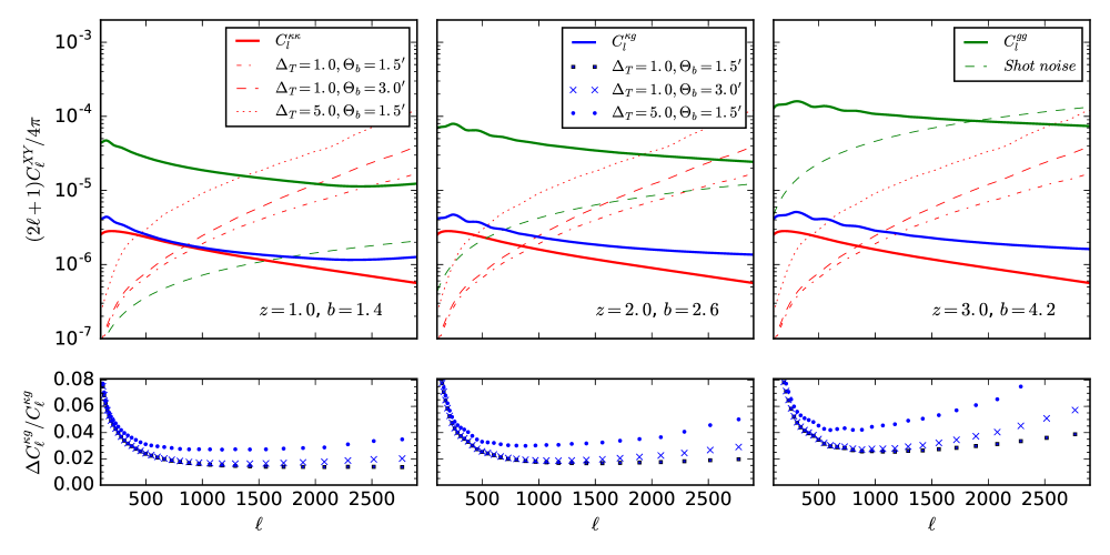
Figure 1: The signal and noise angular power spectra at $z=1$ (left), $z=2$ (middle) and $z=3$ (right). Upper panels: the power spectra for the lensing and galaxy auto-correlations ($\kappa\kappa$ and $gg$) and the cross-correlation ($\kappa g$) for a bin of width $\Delta z=0.5$ and different combinations of noise and beam sizes. The galaxy auto-correlations ($C_{\ell}^{gg}$) assume the halo power spectra of our N-body simulation (§3) but a shot-noise appropriate to the LSST gold sample. The lensing noise is the minimum variance combination of $TT$, $TE$, $EE$ and $EB$ as described in Appendix A. We have assumed the CMB and galaxy survey overlap on 50% of the sky. Lower panels: The fractional error on $C_{\ell}^{\kappa g}$ for bins of $0.1\,\ell$. Future experiments could approach 1% precision on $C_{\ell}^{\kappa g}$ in multiple bins.

Fig. 1 shows the signal and noise angular power spectra as well as the inferred fractional error on the cross-correlation, $C_{\ell}^{\kappa g}$, for some example configurations. We have used the CLASS code [54] to compute the CMB lensing spectra. To make contact with later sections, we have taken the tracer signal levels appropriate for halos of $10^{12}\,h^{-1}M_{\odot}$ in our N-body simulation (see §3) but we use the $dN/dz$ of the LSST gold sample [55] in slices of width $\Delta z=0.5$.

The assumptions and formalism used to estimate the uncertainties is described in Appendix A. In particular the lensing noise is the minimum variance combination of $TT$, $TE$, $EE$ and $EB$, with $\ell_{\rm max}=3000$, 5000 for temperature and polarization respectively. We find that, for a given noise level, the errors in $C_{\ell}^{\kappa\kappa}$ and $C_{\ell}^{\kappa g}$ are quite insensitive to angular resolution in the range $1^{\prime}-3^{\prime}$ FWHM (see also Ref. [19]). The $TT$ contribution also stays fairly constant with map noise levels between $1-5\,\mu$K-arcmin (after foreground cleaning). Below approximately $2\,\mu$K-arcmin noise the $EB$ contribution begins to significantly reduce the uncertainty on $\kappa$. Next-generation CMB experiments are noise-limited in lensing, per $\ell$, beyond $\ell$ of a few hundred but there is still significant constraining power at high $\ell$ because of the many modes which can be averaged together. An experiment such as CMB-S4 would be sample variance limited to just below $\ell=10^{3}$.

The uncertainty in the cross correlation has contributions from CMB map noise and shot noise in the imaging survey. As for the $\kappa$ noise, this is also fairly inensitive to the beam for scales larger than $\ell=2000$, but the fractional errors increase by more than $1.5\%$ for $\ell>1500$ on increasing the map noise from $1\,\mu$K-arcmin to $5\,\mu$K-arcmin. For the cases shown in Fig. 1 the shot-noise is highly subdominant at lower $z$ and so the fractional cross correlation uncertainty is very weakly dependent on the level of shot noise (it would increase by only $\sim 0.5\%$ for a survey one magnitude shallower). However the errors start to depend upon shot noise at the higher redshifts. We note that despite averaging modes in bins of $\Delta\ell=0.1$, the fractional error in $C_{\ell}^{\kappa g}$ reaches a minimum of $1\%$ around $\ell=1500$ at $z=2$ and then starts to increase again. This thus sets the minimum level of accuracy that we need from our model.

Current generation large scale surveys, such as DES, are completely dominated by shot noise at $z=2$ and $z=3$ on scales smaller than $\ell=1000$. Deeper surveys, such as HSC, suffer primarily due to smaller sky coverage and increased sample variance. A future survey like LSST has the combination of depth and area to provide strong constraints to $\ell=1000$ at $z=1$ and $2$, with shot noise becoming important only at higher $z$. There is still significant CMB lensing contribution at high redshift, however, and thus significant potential constraining power. It is therefore worthwhile considering alternative techniques to improve SNR when pushing to higher redshifts. At these redshifts one can efficiently select samples of galaxies using dropout techniques, e.g. $u$-band dropouts for $z\sim 3$ and $g$-band dropouts for $z\sim 4$. Magnitude limited dropout samples naturally produce bands in redshift of about $\Delta z\sim 0.5$ with clustering properties that are similar to normal galaxies at $z=0$ [56, 57]. Using the UV luminosity functions of Ref. [58] reaching a number density at which we are sample variance limited (in $C_{\ell}^{gg}$) to $\ell=2000$ for our $10^{12}\,h^{-1}M_{\odot}$ halos requires an $\mathcal{R}$-band depth of about $24.3$. It might be more efficient to look at $g$-band dropouts (i.e. $z\sim 4$), where it is possible to go fairly deep relatively quickly in the dropout band. Another alternative would be medium or narrow band surveys which are targeted at specific redshift ranges, picking up e.g. Lyman-$\alpha$ emitting galaxies. It is not the purpose of this paper to propose a deeper imaging survey, so we leave this topic for future investigation. Rather we shall take the above to suggest it is possible to achieve percent-level constraints on the cross-correlation over a wide range of $\ell$ and $z$ from future experiments (or by enhancing current surveys). This motivates our development of an appropriate theory for the interpretation of such data.

Throughout this paper we shall follow standard practice and approximate the lensing using the Born approximation, though we shall include non-linear terms in the large-scale densities. As the precision improves it will be necessary to reconsider all such approximations [59, 60] for cross-correlations as well as the auto-spectrum of $\kappa$ and to worry about cleaning out contaminants [61, 5, 62]. Isolating the signal to higher redshift, where the non-linearity is less pronounced, makes the cross-spectrum less sensitive to bispectrum and trispectrum terms than the $\kappa$ auto-spectrum. However by focusing on overdense regions where biased tracers reside the impact of non-linearities is enhanced. How this impacts a cross-correlation measurement from a lensed CMB sky will require further investigation.

2.2 Lightcone evolution: the effective redshift

Once the evolution of $P(k,z)$ is specified, the theory of §2.1 can be used to provide an accurate prediction for the auto- and cross- angular power spectra which are observed. This allows us to compare theory and observation even for sources with broad redshift kernels where we expect significant evolution across the sample. However it is often the case that we wish to interpret the $C_{\ell}$, which involve integrals across cosmic time, as measurements of the clustering strength at a single, “effective”, epoch or redshift. Motivated by Eq. (2.3) we define

$$z_{\rm eff}^{XY}=\frac{\int d\chi\ \left[W^{X}(\chi)W^{Y}(\chi)/\chi^{2}\right]\ z}{\int d\chi\ \left[W^{X}(\chi)W^{Y}(\chi)/\chi^{2}\right]\ \hphantom{z}}$$ (2.6)

such that the linear term in the expansion of $P(k,z)$ about $z_{\rm eff}^{XY}$ cancels in the computation of $C_{\ell}^{XY}$.

We have compared $C_{\ell}^{\kappa g}$ and $C_{\ell}^{gg}$ computed using an evolving $P(k,z)$ to that produced by using $P(k,z_{\rm eff})$ in Eq. (2.3) for several $dN/dz$ shapes and widths, $\Delta z$. Using the evolution of the halo sample of §3 as an example we find the $C_{\ell}$ are within 1.5% for $\Delta z\leq 0.5$ and $\ell>10$ for $1<z<3$. The difference rises quickly beyond $\Delta z=0.5$ and is 5% for $\Delta z=1$. The evolution of $P_{hh}$ we have used as an example is quite strong, since we have focused on a fixed halo mass and thus a tracer whose bias increases strongly with redshift. More gradual evolution of $P(k)$ (e.g. passive evolution) would obviously lead to smaller effects, with no effect in the limit of constant $P(k)$.

In what follows we shall use $\Delta z=0.5$ and approximate our inferences as $P(k,z_{\rm eff})$. Obviously as the width of the slice is reduced the angular clustering of the tracers is enhanced and the approximation of $P(k,z)$ by $P(k,z_{\rm eff})$ improves. However in this limit the shot noise increases as well, and the correlation with the $\kappa$ field decreases rapidly. For increases in $\Delta z$, the cross-correlation increases and the shot-noise drops (as does the signal) but we trade the possibility of multiple independent thin slices in redshifts which can be combined to reduce errors (in quadrature), to a single thick slice with smaller errors. We find that error in the auto-spectra are smaller when using a single thick slice while those in cross spectrum prefer multiple thin slices slices. This opposing trend, coupled with the caveat that one needs a model for the evolution of $P(k)$ in order to interpret the observations from thick slices, makes $\Delta z=0.5$ a suitable choice for our current work.

2.3 Convolution Lagrangian effective field theory (CLEFT)

As argued above, we desire a flexible yet accurate model for the auto- and cross-clustering of biased tracers and the matter in order to exploit the information soon to be available from surveys. Since the observations probe high redshift and relatively large scales, higher order perturbation theory seems a natural choice. In particular Lagrangian perturbation theory and effective field theory, coupled with a flexbile Lagrangian bias model, offer a systematic and accurate means of predicting the clustering of biased tracers in both configuration and Fourier space (e.g. Ref. [40]) making it an ideal tool for modeling cross-correlations of CMB lensing with tracers of large-scale structure. Below we shall present only the Fourier space formalism for brevity, though in some instances configuration space analyses may be preferred. Our formalism naturally handles both views with the same parameters [40] so it can be employed in fitting data in either space.

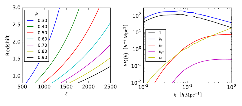
Figure 2: (Left) The mapping between $k$ [in $h\,{\rm Mpc}^{-1}$] and $\ell$ as a function of redshift for the cosmology of our N-body simulation. In the range $1<z<3$, which is our focus, angular scales $\ell<10^{3}$ correspond to the quasi-linear scales easily within the reach of perturbation theory. (Right) Contributions of the various terms in Eq. (2.7) at $z=2$ using the best-fit parameters determined in §3.

The cross-correlation between the matter and a biased tracer, in real space, contains a subset of the terms described in Ref. [40]. Specifically the cross-power spectrum can be expressed as

$$P_{mg}(k)=\left(1-\frac{\alpha_{\times}\,k^{2}}{2}\right)P_{Z}+P_{\rm 1-loop}+\frac{b_{1}}{2}P_{b_{1}}+\frac{b_{2}}{2}P_{b_{2}}+\frac{b_{s^{2}}}{2}P_{b_{s^{2}}}+b_{\nabla^{2}}P_{b_{\nabla^{2}}}+s_{\times}$$ (2.7)

where $P_{Z}$ and $P_{\rm 1-loop}$ are the Zeldovich and 1-loop matter terms, the $b_{i}$ are Lagrangian bias parameters for the biased tracer, $\alpha_{\times}$ is a free parameter which accounts for small-scale physics not modeled by LPT and $s_{\times}$ is a possible “stochastic” contribution. The individual $P_{x}$ can be written as spherical Hankel transforms

$$P_{x}=4\pi\int q^{2}\,dq\ e^{-(1/2)k^{2}(X_{L}+Y_{L})}\left[f_{x}^{(0)}(k,q)j_{0}(kq)+\sum_{n=1}^{\infty}f_{x}^{(n)}(k,q)\left(\frac{kY_{L}}{q}\right)^{n}j_{n}(kq)\right]$$ (2.8)

with the linear Lagrangian correlator decomposed as $A_{ij}^{\rm lin}=\delta_{ij}X_{L}+\hat{q}_{i}\hat{q}_{j}Y_{L}$ and the $f_{x}^{(n)}$ given in [50, 40] (see Appendix B for more details and a simplified model). All of these results assume that the LPT kernels are time-independent. This is an excellent approximation for the density fields at high redshift that we consider [63, 64, 65].

For the halo auto-spectrum the stochastic term includes a contribution from shot noise and can be taken to be scale-independent at the order we work (i.e. a constant). We find that this term is very well predicted by a Poisson shot noise and since we subtract such a term from our “signal” spectra (§3) we can omit it. For the matter-halo cross-spectrum the stochastic term scales as $k^{2}$ as $k\to 0$ (but is unconstrained at high $k$) and is also generally omitted. We have experimented with different forms and values of $s_{\times}$ and find our results are not particularly sensitive to such choices. The fit is slightly improved if we include a constant or a form like $(k/k_{\star})^{2}/[1+(k/k_{\star})^{2}]$ with $k_{\star}\simeq 0.1-0.5\,h\,{\rm Mpc}^{-1}$. This amplitude of this term is never particularly large, and it helps primarily at high $k$. We choose to also omit this term for simplicity, though we note that including an additional constant as a nuisance parameter could help when fitting data. It is also worth noting that in the N-body simulations to which we compare in §3 we may have an additional contribution from the finite sampling of the density field by dark matter particles. A Poisson contribution to the cross-spectrum, $(\bar{n}_{\rm halo}\bar{n}_{\rm dm})^{-1/2}$, would be in the range $10-30\,h^{-3}\,{\rm Mpc}^{3}$ for the samples we discuss in §3 and thus not negligible at high $k$. Thus when comparing to the N-body we could have an additional contribution to $P_{mg}$ which is constant (to lowest order) and potentially as large as the Poisson value above. We assume henceforth that this term is negligble. Clearly a better understanding of the stochastic terms could yield benefits in pushing the model to higher $k$, but awaits further theoretical developments.

The $b_{i}$ represent bias terms (for a recent review of bias see Ref. [66], for a discussion of the advantages of a Lagrangian approach see Ref. [40]). The lowest order term, $b_{1}$, dominates on large scales and is related to the “linear”, scale-independent, Eulerian bias $b=1+b_{1}$. The second term, $b_{2}$, encodes scale-dependence while $b_{s^{2}}$ and $b_{\nabla^{2}}$ encode the dependence of the object density on second derivatives of the linear density field (e.g. a constraint that objects form at peaks). We find we do not need these last two terms at high redshift where our theory performs best, but they could become important to accurately model clustering at higher $k$ [66]. These additional terms could also become more important for samples where assembly bias plays a role, or samples with specific kinds of formation histories, e.g. galaxies selected via color cuts, with strong emission lines or which have more reliable photometric redshifts.

Within the peak-packground split for the Press-Schechter mass function [67] the first two bias parameters are related to the peak height, $\nu$, and the critical density for collapse, $\delta_{c}$, by

$$b_{1}=\frac{\nu^{2}-1}{\delta_{c}}\qquad,\qquad b_{2}=\frac{\nu^{4}-3\nu^{2}}{\delta_{c}^{2}}$$ (2.9)

In this model $b=1$ would correspond to $b_{1}=0$ and $b_{2}=-0.7$, $b=2$ to $b_{1}=1$ and $b_{2}=-0.3$. Note that $b_{2}\to b_{1}^{2}$ as $b_{1}\to\infty$, so the scale-dependence of the bias is predicted to become more pronounced as the bias increases. This expectation is borne out in our fits, however we find that the relationship between $b_{1}$ and $b_{2}$ is not quantitatively very accurate so we treat the $b_{i}$ as free parameters. There is some evidence from N-body simulations that a relationship between the $b_{i}$ does exist [68, 69, 70]. Using such relationships as priors on the parameters could yield benefits for some science goals, as we discuss later. The derivative bias terms, $b_{s^{2}}$ and $b_{\nabla^{2}}$, only become important on small scales and we shall not include them below.

The expression for the auto-spectrum of the biased tracers can be found in Ref. [40] and we shall not reproduce it here. In addition to the terms linear in $b_{1}$, $b_{2}$, etc. it contains quadratic terms like $b_{1}^{2}$, $b_{1}b_{s^{2}}$, and so on. The bias terms, $b_{i}$, are common to the auto- and cross-spectra but the value of $\alpha$ can be different for each spectrum. We denote these as $\alpha_{\times}$ and $\alpha_{a}$, with the subscript $a$ referring to the auto-spectrum.

As we explore below, when comparing to observations involving biased tracers choosing a sophisticated and flexible bias model is essential in order not to introduce errors. In fact the impact of beyond-linear bias parameters is equal in importance to the effects of non-linear gravitational evolution. In the language of EFT, the “cut-off” scale associated with biasing is of order the Lagrangian radius of the halos hosting our tracers. For a fixed halo mass this is a redshift-independent scale. By contrast the cut-off associated with gravitational non-linearity moves to higher $k$ at higher $z$.

Fig. 2 shows the relative contribution to $P_{mh}$ of different terms at $z=2$, using the best fit parameters determined in the next section. We can see that the dominant terms are $P_{Z}$, $P_{\rm 1-loop}$ and $P_{b_{1}}$. The other terms are subdominant, but can affect the predictions at the high accuracy which will be demanded by future observations.

3 Comparison with N-body simulations

In order to validate our approach, we compare our analytic models to the cross-power spectrum between halos and dark matter measured in N-body simulations. For this purpose we make use of 10 simulations run with the TreePM code of [71]. Each simulation employs the same ($\Lambda$CDM) cosmology but with a different random number seed chosen for the initial conditions. These simulations have been described in more detail elsewhere [72, 73, 50], but briefly they were performed in boxes of size $1380\,h^{-1}$Mpc with $2048^{3}$ particles and modeled a $\Lambda$CDM cosmology with $\Omega_{m}=0.292$, $h=0.69$, $n_{s}=0.965$ and $\sigma_{8}=0.82$. We use outputs at $z=1$, $2$ and $3$ to sample the range of most interest for cross-correlations with CMB lensing. For each output we compute the real-space auto-spectra of the halos and matter and the cross-spectrum between the halos and matter for friends-of-friends ($b=0.168$) halos with $10^{12.0}<M<10^{12.5}\,h^{-1}M_{\odot}$. The power spectra were computed on a $2048^{3}$ grid, using cloud-in-cell interpolation, and the spectra were corrected for the window function of the charge assignment and for (Poisson) shot-noise. The number density of halos was $1.70\times 10^{-3}\,h^{3}\,{\rm Mpc}^{-3}$ at $z=1$, $1.0\times 10^{-3}\,h^{3}\,{\rm Mpc}^{-3}$ at $z=2$ and $3.8\times 10^{-4}\,h^{3}\,{\rm Mpc}^{-3}$ at $z=3$.

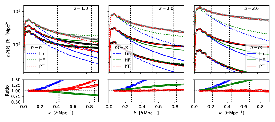
Figure 3: A comparison of the analytic model to the results from N-body simulations. The upper panels show $k\,P(k)$ for the matter auto-spectrum (lower set of dashed lines and squares) the halo-matter cross spectrum (middle set of solid lines and circles) and the halo-halo auto-spectrum (upper set of dotted lines and diamonds) with shot-noise subtracted. The points show the N-body results (in real space) at (left) $z=1$, (middle) $z=2$ and (right) $z=3$. Blue lines show the linear theory with a constant bias, the green lines show the HaloFit [74] spectra with constant bias while the red lines show the perturbation theory (PT) predictions. In the lower panel we show the ratio of the N-body cross-spectra ($P_{mh}$) to each of the linear theory, HaloFit and PT predictions on an expanded $y$-scale. For the PT predictions we also show the ratio for the auto-spectra (red diamonds). The vertical dotted lines mark $\ell=1000$, $2000$ and $3000$ [missing in the $z=1$ panel].

Fig. 3 compares the N-body results to the CLEFT results of the previous section, and to the HaloFit fitting function [74]. Upper panels show the comparison over the full range while the lower panels show the ratio of the N-body results to each of the theoretical models, with an expanded $y$-axis scale to highlight small deviations. In the upper panel the squares show the matter power spectrum, where we see that the N-body departs significantly from linear theory even at $k\simeq 0.25\,h\,{\rm Mpc}^{-1}$: $P/P_{L}=1.15$, $1.07$ and $1.04$. This is consistent with the level of power, as measured by the dimensionless power spectrum: $\Delta^{2}(k=0.25\,h\,{\rm Mpc}^{-1},z)=0.45$, $0.20$ and $0.11$ at $z=1$, $2$ and $3$. Another measure of the non-linear scale is the 1D, rms Zeldovich displacement, $\Sigma$. At $k=0.25\,h\,{\rm Mpc}^{-1}$ the product $k\Sigma$ is $0.9$, $0.6$ and $0.5$ at $z=1$, $2$ and $3$. Unlike linear theory, the agreement between 1-loop perturbation theory and the N-body results is very good to quite high $k$: within 1% out to $k=0.3$, $0.4$ and $0.6\,h\,{\rm Mpc}^{-1}$ for $z=1$, 2 and 3 and within 5% to $k=0.5\,h\,{\rm Mpc}^{-1}$ at $z=1$ and $k\simeq 0.7\,h\,{\rm Mpc}^{-1}$ at $z\geq 2$. For comparison the updated HaloFit fitting function [74] fits the N-body matter power spectrum almost within the quoted accuracy (5% for $k<1\,h\,{\rm Mpc}^{-1}$ and $0<z<10$) with a maximum deviation of $6\%$ in the $z=3$ output. A recent comparison of the performance of different fitting functions for the matter power spectrum can be found in Ref. [75].

The results of direct relevance for our purposes are the halo-matter cross-correlations and the halo-halo auto-correlations, also shown in the upper panel of Fig. 3. We perform a joint fit to the two spectra, so that the relevant bias terms are self-consistent. Unlike later sections, in these fits we put most of the weight at low $k$ (enforcing a good match at low $k$ and to reduce over-fitting) and we allow $b_{s^{2}}$ to be free to test it has a small impact. Concentrating on the cross-spectrum, the lower panels show the ratio N-body/model for CLEFT and the newer HaloFit of Ref. [74] with an expanded $y$-axis. We see that the best-fitting perturbation theory model matches the N-body data at the few percent level out to $\ell\simeq 750$ for $z=1$ and to $\ell\simeq 2000$ for $z=2$ and 3. Key to this level of agreement is a flexible bias model. The constant bias, linear theory results are not accurate for $k\geq 0.1\,h\,{\rm Mpc}^{-1}$ even at these high redshifts. HaloFit improves over linear theory by quite a bit, but a scale-independent bias is not a good model for the clustering of these halos at $1<z<3$ even at $\ell<10^{3}$. The errors introduced by assuming a scale-independent bias can exceed 10% on quasi-linear scales.

Fig. 4 shows the scale dependence of the bias estimated from the cross- and auto-spectra. As the redshift increases and halos of a fixed mass become more biased the scale dependence of the bias becomes more pronounced and the scale dependence differs more markedly between the auto- and cross-spectra. This means that a model based purely upon the dark matter power spectrum becomes increasingly less accurate, even though that spectrum itself is better approximated by linear theory.

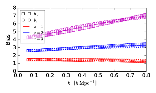
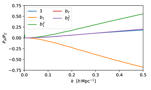
Figure 4: (Left) The bias terms, estimated from the cross- and auto-spectra, for our N-body halos at $z=1$, $2$ and $3$. Motivated by Eq. (4.2) we define $b_{\times}(k)=P_{hm}(k)/P_{mm}(k)$ and $b_{a}(k)=[P_{hh}(k)/P_{mm}(k)]^{1/2}$. Note that the bias is scale dependent, but the scale dependence is different for the cross- and auto-spectra. Both the scale dependence and the difference become more pronounced as the bias increases. (Right) The non-linear and bias contributions to the cross-correlation coefficient, $\rho=P_{hm}/\sqrt{P_{hh}P_{mm}}$, as a function of $k$ (see Eq. 4.4) assuming no shot noise. The difference of $\rho^{2}$ from unity grows to high $k$ due to non-linear structure formation (the “1” term) and the complexities of bias (the other terms) as discussed in §4.

4 Measuring $P_{mm}(k,z)$

A proper accounting of the growth of large scale structure through time is one of the main goals of observational cosmology. A key quantity in this program is the matter power spectrum as a function of redshift. Here we discuss how the cross-correlation can be combined with the convergence or tracer auto-correlation to measure $P_{mm}(k,z)$. To illustrate this measurement we pretend that the amplitude of the linear theory spectrum ($\sigma_{8}$) was unknown, holding its shape fixed for simplicity, and then attempt to recover its value from the mock data.

First we model the auto and cross angular power spectra of a particular sample in an individual redshift slice. Following §2.2 we take the spectra to be redshift independent over the width of the slice, and assume that $dN/dz$ is perfectly known. In such a situation we may schematically think of measuring the matter power spectrum as:

$$P_{mm}(k)\sim\frac{\left[C^{mg}_{\ell=k\chi}\right]^{2}}{C^{gg}_{\ell=k\chi}}$$ (4.1)

Operationally we perform a joint fit to the combined data set, including correlations and possibly some parameters to account for systematic errors. With only the auto-spectrum there is a strong degeneracy between $\sigma_{8}$ and the bias parameters (particularly $b_{1}$). However the matter-halo cross-spectrum has a different dependence on these parameters and this allows us to break the degeneracy and measure $\sigma_{8}$.

We compare the ability of two models to fit $C_{\ell}^{\kappa g}$ and $C_{\ell}^{gg}$ with errors appropriate to three different experimental configurations. Our fiducial setup is (1) that of proposed future experiments with depth equivalent to the LSST gold sample, which corresponds to the limiting magnitude $i_{\rm lim}=25.3$, combined with a CMB experiment having $1\,\mu$K-arcmin noise and a beam of $1.5^{\prime}$. To see how noise in imaging and CMB surveys impact our fits, we also do the analysis for experimental configurations corresponding to (2) higher shot noise, which is modeled by using a limiting magnitude $i_{\rm lim}=24.3$ while keeping CMB noise fixed, and another setup corresponding to (3) a CMB experiment having $5\,\mu$K-arcmin noise and a beam of $3^{\prime}$ with $i_{\rm lim}=25.3$. We always assume the overlap of the CMB and imaging surveys is $f_{\rm sky}=0.5$. Our errors scale as $f_{\rm sky}^{-1/2}$.

We have generated mock data, $C_{\ell}^{\kappa g}$ and $C_{\ell}^{gg}$, assuming $P_{mh}(k)$ and $P_{hh}(k)$ from our N-body simulations at the central redshift of our slice, with $dN/dz$ appropriate to LSST survey and correspoding $i_{\rm lim}$. We work in redshift slices of $\Delta z=0.5$ around the central redshift (e.g. $1.75<z<2.25$ for $z=2$) and fit these mock data using two models.

Our fiducial model is the perturbation theory described in §2.3, allowing $\sigma_{8}$, $b_{1}$, $b_{2}$, $\alpha_{\times}$ and $\alpha_{a}$ to vary. As a comparison, and because it has been so widely used in the literature, we use a model based on the HaloFit fitting function for $P_{mm}(k)$. As expected from Fig. 3, assuming a scale-independent bias is insufficient to analyze any of the experimental configurations we consider – the results are biased by many standard deviations. To give some flexibility we allow the bias to be scale-dependent. One choice, motivated by peaks theory, is to use $b(k)=b_{10}^{E}+b_{11}^{E}k^{2}$ [66] where we have superscripted the $b_{ij}$ with an $E$ to indicate their Eulerian nature and to distinguish them from the $b_{i}$ in Eq. (2.7). We found that this choice alone does not provide a good fit to our N-body data, as expected from Fig. 4. Motivated by Fig. 4, but as a purely phenomenological choice, we add a term linear in $k$ to our bias model. Then

$$P_{mh}(k) = \left[b_{10}^{E}+b_{1\frac{1}{2}}^{E}k+b_{11}^{E}k^{2}\right]P_{HF}(k)$$

$$P_{hh}(k) = \left[b_{10}^{E}+b_{1\frac{1}{2}}^{E}k+b_{11}^{E}k^{2}\right]^{2}P_{HF}(k)$$ (4.2)

with $P_{HF}$ the HaloFit fitting function for the matter auto-spectrum and free parameters $\sigma_{8}$, $b_{10}^{E}$, $b_{1\frac{1}{2}}^{E}$ and $b_{11}^{E}$.

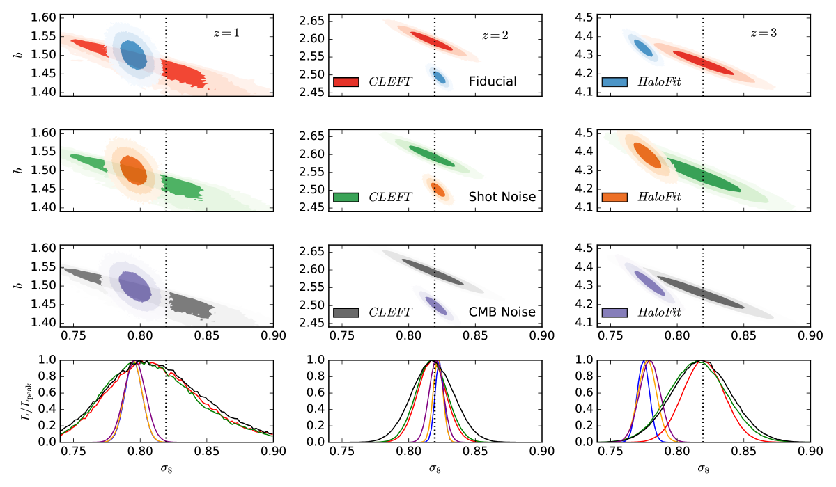
Figure 5: Performance of the CLEFT perturbation theory model and the phenomological HaloFit model at 3 different redshifts, $z=1$, $2$, and $3$. The top row show marginalized parameter distributions of $b$ and $\sigma_{8}$ for fits to $C_{\ell}^{\kappa g}$ and $C_{\ell}^{gg}$ for proposed future experiment, while the second and third rows show the same distributions but for increased shot noise and CMB experimental noise respectively (see text). The fits are restricted to $\ell<2000$. The definition of $b$ is different for the two models, so the values should not be compared directly. The last row shows the normalized posterior for $\sigma_{8}$ normalized to be 1 at the peak, with the vertical, black, dotted line marking the “true” value ($\sigma_{8}=0.82$) used in the simulations.

To evaluate the posteriors we run Monte Carlo Markov Chains (MCMC) using the emcee package [77] for both models at $z=1$, $2$ and $3$, for all three experimental configurations. Unless specified otherwise, we will quote the bias in the $50^{\rm th}$ percentile values (i.e. median) of these fits and $1\,\sigma$ errors based on the $16^{\rm th}$ and $84^{\rm th}$ percentile values, but we have verified that using other statistics such as mean or standard deviations does not change the numbers. We restrict the fits to $\ell_{\rm max}=2000$, even though the experiments have useful measures of $C_{\ell}^{\kappa g}$ and $C_{\ell}^{gg}$ beyond this value. This is based on the discussion in §2.3 and also because we found that going to higher $\ell$ does not improve the fits significantly (see below).

Fig. 5 compares the marginalized likelihoods in the $\sigma_{8}-b$ plane (for the perturbation theory model we define $b=1+b_{1}$ while for the phenomenological model $b=b_{10}^{E}$). At $z=2$ and $3$ the CLEFT model returns unbiased constraints on $\sigma_{8}$ for $\ell_{\rm max}=2000$. In fact, we find that we can extend the fits to $\ell_{\rm max}=3000$ without biasing our recovered $\sigma_{8}$ by $1\,\sigma$. Including higher $\ell$ reduces the $1\,\sigma$ errors from $1.25\%$ to $1\%$ at $z=2$, but it also increases the bias from $0.3\%$ to $0.5\%$. At $z=3$, the errors are $1.8\%$ and $1.6\%$ with a bias of $0.05\%$ and $0.1\%$ respectively for the two $\ell_{\rm max}$. For $z=1$ the CLEFT model is biased whenever $\ell_{\rm max}>500$, which is not unexpected given the discussion in §3. We expect this bias would increase further if we pushed below $z=1$. We shall discuss improvements to the model which could extend the reach to lower redshift later.

The HaloFit model provides much tigher constraints on $\sigma_{8}$ than CLEFT ($1\,\sigma$ errors of $0.34\%$ compared to $1.25\%$ at $z=2$), however the estimates are biased by many $\sigma$ when fit to the same $\ell_{\rm max}=2000$ as CLEFT ($0.63\%$, or $2\,\sigma$ compared to $0.33\%$, or $(1/3)\sigma$, at $z=2$). This is initially surprising, given that the claimed $k$-range of validity of HaloFit is larger than for perturbation theory, but reinforces the necessity of a sophisticated bias model and the high level of precision demanded of fitting functions if they are to be used to interpret future data. We find that at $z=2$ it is possible to get an unbiased estimate of $\sigma_{8}$ by reducing $\ell_{\rm max}$ to $1500$, however even this is not sufficient at $z=1$ and $3$. In fact, at $z=1$ HaloFit breaks down at the same scale as CLEFT ($\ell=500$): the central value is as biased as for CLEFT but since the error bar is significantly smaller the central value is $3\,\sigma$ away from the truth.

We also find that at $z=2$, where the galaxy auto-clustering is well above the shot noise, going one magnitude shallower does not significantly increase the uncertainty on $\sigma_{8}$ (from $1.25\%$ to $1.36\%$). Our fits are more sensitive to CMB noise. Increasing the noise to $5\,\mu$K-arcmin increases our errors to $1.75\%$. However at $z=3$, where the survey becomes shot noise dominated at $\ell>1800$, we are equally sensitive to CMB noise and increased shot noise, with $1\,\sigma=2.5\%$ for both of them compared to $1.8\%$ for the fiducial survey.

The performance of HaloFit times a polynomial bias function clearly highlights the necessity of a more sophisticated modeling approach in order to make use of the massive amounts of cosmological information which will be provided by future CMB and imaging surveys. Even with the additional linear term introduced to better model bias, HaloFit is not able to fit scales where the data still have significant constraining power. Further, we note that for halos of $M_{h}\simeq 10^{12}\,h^{-1}M_{\odot}$, $z=2$ seems to be a sweet spot where the matter distribution is not highly non-linear while at the same time the observed tracers are not very highly biased. We expect such a sweet spot to exist for any halo mass, since halos are more biased to higher redshifts while the clustering is more non-linear to lower redshifts. To push the sweet spot to higher redshift requires selecting lower mass halos, which generally host lower luminosity galaxies. Given these factors it is not surprising that the performance of HaloFit deteriorates in either direction from $z=2$. On the other hand, that the performance of CLEFT remains more or less unchanged on going from $z=2$ to $z=3$, suggests that the bias model employed is already flexible enough, even though we have not used the additional bias parameters $b_{s^{2}}$ and $b_{\nabla^{2}}$. This is also suggested by the fact that the CLEFT best fits for $\sigma_{8}$ are obtained when both $C_{\ell}^{\kappa g}$ and $C_{\ell}^{gg}$ are fit to same $\ell_{\rm max}$. The quadratic dependence on bias in $C_{\ell}^{gg}$ compared to the linear dependence in $C_{\ell}^{\kappa g}$ does not lead to break down at lower $\ell$. By working to the same $\ell_{\rm max}$ for both statistics we are able to better break the parameter degeneracies.

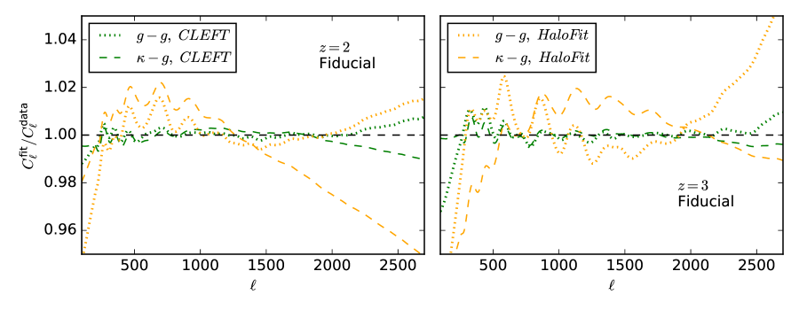
Figure 6: Comparison of the fit to $C_{\ell}^{\kappa g}$ and $C_{\ell}^{gg}$ and the data for the best fits of the CLEFT model and the phenomological HaloFit model at $z=2$ (left) and $3$ (right) for our fiducial experiment (see text). The fits use $\ell_{\rm max}=2000$.

In Fig. 6 we also compare the data and the fits at the level of power spectra. We show the best fits at $z=2$ and $z=3$ for the fiducial experiment. Despite fitting only up to $\ell_{\rm max}=2000$, the best fitting CLEFT power spectra are well within $1\%$ of the data on all scales of interest ($200<\ell<2700$). This is below the statistical error in the data. Such good agreement may be partly coincidence and reflect some over-fitting, but reinforces how robust the results we obtain are to the exact choice of fitting range etc. By contrast the HaloFit fits start to diverge beyond $\ell\simeq 1800$ and have $\sim 2\%$ excursions on intermediate scales. The fits are qualitatively similar for other cases, which we omit for brevity. Another view of the impact of the differences highlighted in Fig. 6 is that the $\chi^{2}$ of the best fitting CLEFT models is 40 (60) lower than that of the best fitting HaloFit models at $z=2$ (3) despite having only one additional degree of freedom.

The CLEFT model has several free parameters and it is straightforward to see the cost that is paid in terms of error budget due to marginalizing over extra parameters. In Fig. 7, we show the error in $\sigma_{8}$ as the function of $\ell_{\rm max}$ to which we fit the model. We always marginalize over the EFT parameters, but investigate the impact of tight priors on the bias parameters. The model used above corresponds to the green curve, marginalizing over $b_{1}$, $b_{2}$, $\alpha_{a}$ and $\alpha_{\times}$. We note that including one extra bias parameter ($b_{2}$) over linear bias ($b_{1}$) does not increase the error more than $0.5\%$. As the above discussion makes clear, however, a proper bias model does drastically reduce the bias in the fits (not shown in this Fisher calculation). The situation changes as we marginalize over additional bias parameters, e.g. $b_{s^{2}}$. Due to the degeneracies introduced, the fit to any given $\ell$ becomes less constraining.

The above is the most natural combination of data for photometric surveys at high $z$. For completeness we remark upon two other possibilities. (1) If redshifts are available for the tracer sample then one can fit the multipoles of the redshift-space power spectrum in order to obtain better constraints on the parameters and an independent constraint on the amplitude. The formalism of §2.3 allows such a fit within the same parameter-set as the current study. One advantage of using the 3D clustering is that there are more modes so we can work at larger scales with the same statistical constraining power. Another advantage is that the anisotropy of the clustering gives another measure of $\sigma_{8}$. A disadvantage is the need to model effects such as fingers-of-god. We leave such an investigation to future work.

(2) Another route to measuring the power spectrum amplitude, though without the redshift specificity, is through $C_{\ell}^{\kappa\kappa}$. While the auto-spectrum of the tracers is likely to have higher signal-to-noise ratio than the auto-spectrum of $\kappa$ it may be that systematics in the tracer spectrum or complications of the bias model favor using $C_{\ell}^{\kappa\kappa}$. In this case the perturbation theory of §2.3 is not directly applicable, since the integral for $C_{\ell}^{\kappa\kappa}$ probes low redshifts and high $k$ values. However, if the low $z$ contribution to $C_{\ell}^{\kappa\kappa}$ can be “cleaned” by using a tracer of the density field at low redshift (e.g. LSST galaxies) then the power spectrum of the cleaned map may be amenable to computation using our formalism. Such a cleaned map may also have smaller contributions from intrinsic bispectrum terms due to non-linear structure formation [59].

If we clean the $\kappa$ map using a biased tracer, the power spectrum of the residual field can be written

$$C_{\ell}^{\rm clean}=\sum_{a}C_{\ell,a}^{\kappa\kappa}\left(1-\rho_{a}^{2}\right)$$ (4.3)

where $C_{\ell,a}^{\kappa\kappa}$ is the contribution to $C_{\ell}^{\kappa\kappa}$ from redshift slice $a$ and $\rho_{a}^{2}=(C_{\ell,a}^{\kappa g})^{2}/C_{\ell,a}^{\kappa\kappa}C_{\ell,a}^{gg}$ is the cross-correlation coefficient (squared) for slice $a$. The $C_{\ell,a}^{gg}$ appearing in $\rho^{2}$ is to be interpreted as a “total” spectrum, including shot noise, such that having no galaxies in the slice sends $\rho\to 0$. We can estimate $1-\rho^{2}$ using our perturbative model. If we treat the EFT and bias terms perturbatively, in the spirit of Ref. [40], then $1-\rho^{2}$ only has contributions from 1-loop terms

$$\rho^{2}\approx\frac{(P^{mh})^{2}}{P^{mm}P^{hh}}=1-\frac{b_{1}^{2}}{(1+b_{1})^{2}}\sum_{A}\rho_{A}^{2}\frac{P_{A}}{P_{Z}}-\frac{{\rm const}}{(1+b_{1})^{2}P_{Z}}$$ (4.4)

where $\rho_{A}^{2}$ are coefficients and $P_{A}$ are 1-loop power spectra, both given in Table 1. The last term, containing the “const”, is the leading stochastic contribution obtained by expanding the terms in $P^{hh}$. Alternatively, this leading stochastic (constant) contribution could be treated non-perturbatively, keeping it in the denominator of the $1/P^{hh}$ expansion, which would in turn affect all the rest of the terms in the sum above. Note that the degree of decorrelation is dependent upon the non-linear nature of the bias model, small-scale physics and the shot noise, as expected. The quantities $P_{A}$ are all 1-loop in our perturbation expansion, and $P_{A}/P_{Z}\to 0$ as $k\to 0$ indicating that $\rho^{2}\to 1$ on large scales if the shot-noise is sufficiently small. The fields begin to decorrelate when the 1-loop corrections become important, and the degree of decorrelation is larger when the objects are more biased (as expected). Again, we leave investigation of this possibility to future work.

$A$	$\rho_{A}^{2}$	$P_{A}$	$A$	$\rho_{A}^{2}$	$P_{A}$
$1$	1	$P_{1-{\rm loop}}$	$b_{s^{2}}$	$b_{s^{2}}/b_{1}$	$2P_{b_{1}b_{s^{2}}}-P_{b_{s^{2}}}$
$b_{1}$	-1	$P_{b_{1}}-2P_{Z}$	$b_{2}b_{s^{2}}$	$b_{2}b_{s^{2}}/b_{1}^{2}$	$P_{b_{2}b_{s^{2}}}$
$b_{1}^{2}$	1	$P_{b_{1}^{2}}-P_{Z}$	$b_{s^{2}}^{2}$	$(b_{s^{2}}/b_{1})^{2}$	$P_{(b_{s^{2}})^{2}}$
$b_{2}$	$b_{2}/b_{1}$	$P_{b_{1}b_{2}}-P_{b_{2}}$	$\alpha$	$2\alpha_{\times}-\alpha_{m}-\alpha_{a}$	$k^{2}P_{Z}$
$b_{2}^{2}$	$(b_{2}/b_{1})^{2}$	$P_{b_{2}^{2}}$

Table 1: Coefficients, $\rho_{A}^{2}$, and 1-loop power spectra, $P_{A}$, for the correlation coefficient of Eq. (4.4).

5 The redshift distribution

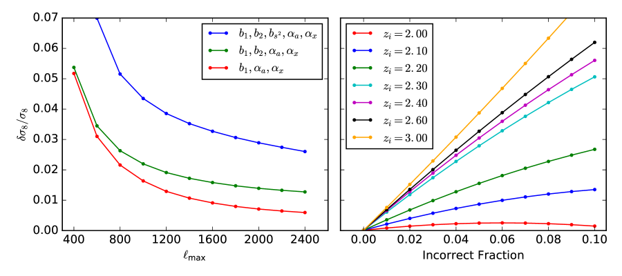
Figure 7: Fisher analysis to predict error on $\sigma_{8}$. The left panel shows hows the error incurred in $\sigma_{8}$ due to marginalizing over extra parameters that are used in CLEFT model as a function of $\ell_{\rm max}$ to which we fit the data. Right panel shows the error in $\sigma_{8}$ due to incorrect $dN/dz$, modeled by adding a Gaussian bump of $FWHM=0.1$ in $z$ centered at redshift $z_{i}$ to the fiducial LSST $dN/dz$ in a slice of width $\Delta z=0.5$ centered at $z=2$. The $x$-axis shows the fraction of sources misidentifed in the LSST sample.

One of the advantages of a cross-correlation is that it isolates the contribution to the lensing signal arising from a small redshift interval, enabling a study of redshift evolution. Such an analysis, however, relies on being able to choose sources which have some known or desired redshift distribution. In this section we look at how accurately we need to determine $dN/dz$ in order to not be limited by this uncertainty.

A change in $dN/dz$ has two effects: it changes the mix of redshifts which contribute to $C_{\ell}$ and it changes the mix of scales ($k$ values) which contribute to a given $\ell$. The change to $C_{\ell}^{\kappa g}$ is linear in $dN/dz$ while the change in $C_{\ell}^{gg}$ is quadratic. We will assess the impact of these changes using a linear approximation, where an error in $dN/dz$ is assumed to be small. In the small-error limit a bias in the data, $\delta d_{n}$, leads to biases in the parameters, $p_{\alpha}$, of:

$$\delta p_{\alpha}=F^{-1}_{\alpha\beta}\frac{\partial\mu_{m}}{\partial p_{\beta}}C^{-1}_{mn}\delta d_{n}$$ (5.1)

where $C$ is covariance matrix of the data, $\mu$ is the model prediction and $F$ is the corresponding Fisher matrix. In the spirit of the last section, we shall focus on the bias introduced in $\sigma_{8}$ assuming

$$\frac{dN}{dz}=(1-f)\left(\frac{dN}{dz}\right)_{1}+f\left(\frac{dN}{dz}\right)_{2}$$ (5.2)

where $(dN/dz)_{2}$ is offset from $(dN/dz)_{1}$ by a varying amount and $f$ is the fraction of sources misidentified in the survey. The largest derivatives, $d\mu_{m}/dp_{\alpha}$, are for $p=\sigma_{8}$ and $b_{1}$ so we shall specialize to the $2\times 2$ Fisher matrix.

Our toy model for $dN/dz$ is to take $(dN/dz)_{1}$ as the LSST-like distribution cut to $1.75<z<2.25$ while introducing a Gaussian $(dN/dz)_{2}$ of FWHM $=0.1$ centered at $z_{i}$. We use the N-body $P(k,z)$ of our $10^{12}\,h^{-1}M_{\odot}$ halo sample to calculate $\delta d_{n}$ and propagate the bias to $\sigma_{8}$ using Eq. (5.1). Fig. 7 shows this fractional error as a function of fraction of misidentified sources (defined as the fraction of total galaxies in the Gaussian), at different values of $z_{i}$. We expect these errors to asymptote with increasing $z_{i}$, since in the extreme case of $z_{i}\rightarrow\infty$, the error in $\delta d_{n}$ should be equal to the error due to reduction in total number of sources.

We note in passing that our formalism could in principle be used to constrain $dN/dz$ at the same time as fit for the model parameters. Since the formalism naturally encompasses cross-correlations between biased tracers in real and redshift space a particularly interesting case would be to constrain $dN/dz$ through cross-correlations with a spectroscopic survey (e.g. Ref. [78] and references therein) while simulataneously fitting the $\kappa-$tracer statistics. We leave investigation of this possibility for future work.

6 Conclusions

A new generation of deep imaging surveys and CMB experiments offers the possibility of using cross-correlations to test General Relativity, probe the galaxy-halo connection and measure the growth of large-scale structure. However improvements in data require concurrent improvements in the theoretical modeling in order to reap the promised science. We have investigated the use of Lagrangian perturbation theory to model cross-correlations between the lensing of the CMB and biased tracers of large-scale structure at high $z$.

Ever lower map noise levels improve the fidelity of CMB lensing maps, with the improvement becoming particularly significant once the noise in the foreground-cleaned maps reaches $\sim 2\,\mu$K-arcmin and the $EB$ spectra dominate. With such improvements maps of the lensing convergence will go from being noise dominated above $\ell\sim 10^{2}$ to noise dominated only above $\ell\sim 10^{3}$, an increase of two orders of magnitude in the number of high signal-to-noise modes and hence useable information. On a similar timescale dramatic increases in the depth and fidelity of optical imaging over large sky areas will come from a next generation of surveys, allowing probes of higher redshift galaxies where the CMB lensing kernel peaks. The combination of these two advances enables multiple science goals through cross-correlations.

We have argued above that the particular scales and redshifts which contain much of the cosmological information in cross-correlations can be modeled using cosmological perturbation theory. This extends the highly successful linear perturbation theory analysis of primary CMB anisotropies which has proven so impactful. It provides a first-principles approach with a sophisticated treatment of bias for the halos and galaxies which are directly observed by the imaging surveys.

In fact, a flexible and sophisticated bias model is critically important in modeling CMB lensing-galaxy cross-correlations. We show that the commonly used scale-independent bias times matter power spectrum approach will be completely inadequate to analyze upcoming surveys, and that simply extending the bias to a polynomial in $k$ does not solve the issue. Rather a proper modeling of the non-linear effects of bias is essential. In fact, in many ways a proper accounting for the complexities of bias is more important than the effects of non-linear structure growth on the matter power spectrum at high $z$ where the CMB lensing kernel peaks. Since the non-linear scale shifts to smaller scales at high $z$, while the Lagrangian radius of a fixed mass halo remains constant, the complexities of bias will only become more relevant at higher $z$.

Comparing the clustering of halos in a series of N-body simulations to our perturbative model, we found that the auto- and cross-clustering of halos above $z=2$ could be well described up to $\ell=2000$ using only two (Lagrangian) bias parameters. While the formalism has been extended to include higher order terms, they were not necessary for the tracers and scales we investigated.

As an example of the science enabled by cross-correlations, we reconstructed the amplitude of the matter power spectrum ($\sigma_{8}$) from the combination of $C_{\ell}^{\kappa g}$ and $C_{\ell}^{gg}$ for some hypothetical experiments. We found that constraints on $\sigma_{8}$ improved slowly beyond $\ell=2000$, and that our fits became biased if we fit the N-body data to higher $\ell$. Unless the modeling can be improved, or if the scale dependence of the bias is partially degenerate with changes due to $\sigma_{8}$ above $\ell=2000$, gains in experimental sensitivity at high $\ell$ will not advance this science goal. For our $10^{12}\,h^{-1}M_{\odot}$ halo sample and slices of width $\Delta z=0.5$ the optical survey is shot-noise limited at $\ell=2000$ for $160$, $390$ and $680$ galaxies per deg² at $z=1$, 2 and 3. The CMB lensing becomes noise dominated beyond $\ell=10^{3}$ at sensitivities of $\sim 5\,\mu$K-arcmin for a wide range of beam sizes. While it is relatively forgiving of map depth and angular resolution, like most cross-correlation science the uncertainty scales as $f_{\rm sky}^{-1/2}$, preferring large sky coverage, overlapping other surveys. We found that cross-correlations of the sort enabled by LSST and CMB-S4 would enable percent level measurements of $\sigma_{8}$ in multiple redshift bins. Deeper imaging would allow us to extend these measurements all the way to $z\simeq 6$.

We have shown that a scale-independent, or “linear”, bias does not provide a good model for $k>0.1-0.2\,h\,{\rm Mpc}^{-1}$ at any redshift we have studied (see Fig. 3). This is at odds with the assumptions of Ref. [19] in their forecasts. Those authors assume linear bias works to $k\simeq 0.6\,h\,{\rm Mpc}^{-1}$ at all redshifts ($2\pi\chi/\ell>10\,h^{-1}$Mpc). While the conclusions of Ref. [19] on shear calibration are very likely unchanged (they can achieve the LSST shear calibration requirements with only cross- and auto-spectra of shears in any case) it would be interesting to revisit these forecasts with a more flexible bias model. Such an investigation, and an exploration of the degeneracies introduced, is beyond the scope of this paper although we give some additional comments below.

The contributions of the different biasing terms in Eq. (2.7) are formally independent, however if we keep all of the terms there is a danger of over-fitting. For a fixed precision, e.g. 1%, the different contributions can exhibit approximate degeneracies so that a subset of the terms can mimic the effects of the rest. In principle adding higher order statistics, like the bispectrum, can help break approximate degeneracies. In absence of such additional information, an alternative is to reduce a number of independent terms. This is the approach we have adopted in our analysis: keeping the $b_{1}$ and $b_{2}$ bias parameters. We note that the values of these parameters should now be understood in the ‘effective’ sense, since they also partially take the role of $b_{s^{2}}$ and $b_{\nabla^{2}}$ terms, which could additionally change the numerical values of these parameters from the peak-background split estimates given by Eq. (2.9).

In addition to the biasing parameters we have considered so far, effects related to baryonic physics leaking in from the small scales can affect the galaxy clustering even on fairly large scales. Additionally, we can also consider relative-density and relative-velocity perturbations that can also potentially appear on large scales. These baryonic effects can be added to the biasing description, considering them as an additional species adding to the full set of symmetry allowed terms for the galaxy overdensity [79, 80], starting from additional relative-density $\delta_{\rm bc}$ and relative-velocity $\theta_{\rm bc}$ perturbation. In addition to these effects we have also higher order contributions starting from the relative velocity effects [81, 79, 82, 80], though these terms have also been recently studied and constrained to be a rather small effect [83, 84] relative to the rest of the terms. We also note that similar effects described by the general formalism presented in [79, 80] could also be adapted to describe effects of cosmic neutrinos or fluctuating dark energy models [85] on mildly-nonlinear scales. We note that the CLEFT formalism used in this paper can be readily extended to include these additional biasing terms.

Finally we remark on some directions for future development. While we have focused here on a single population of tracers, there are significant gains which can be had by using multi-tracer techniques [86, 87, 88]. The formalism described above can be straightforwardly extended to the multi-tracer case, including the decorrelations which occur at high $k$. The inclusion of low mass neutrinos into the formalism is straightforward, and there are extensions for models with modifications to General Relativity [89, 90]. In the near future the demands on the theory are significantly relaxed, and simpler approximations can perform adequately. We discuss one such approach in Appendix B. In the other direction, we have focused throughout on 1-loop perturbative predictions with a Lagrangian bias model which is $2^{\rm nd}$ order in the linear density field. We saw that at high redshift the uncertainties due to the bias model dominated over the non-linearities in the matter clustering. However this situation changes as we move to lower redshift and the clustering becomes more non-linear. There is no reason, in principle, why one cannot continue the expansion to higher order in order to deal with this. Ref. [91] presents the 2-loop EFT calculation (in Eulerian PT) for the matter power spectrum. At this order there are 6 EFT counter terms which need to be fixed. These terms are highly degenerate, and Ref. [91] discuss some ways to reduce this number. It is an open question whether one needs to work at higher order in the bias expansion. If so, this would add additional parameters. However at lower redshift we expect to be using galaxies of lower bias and we have the ability to adjust our samples so as to minimize the scale-dependence of their bias so it is likely that we can stay with the same order as used above. If we keep all of the EFT terms then even at the same order in the bias expansion we would be fitting 9 parameters to the data, rather than our current 4 (plus $\sigma_{8}$). It remains to be seen whether the increase in information afforded by going to smaller scales using higher order perturbation theory overcomes the need to introduce more free parameters in the fit. On the other hand, one can use priors from N-body simulations or fitting functions to partially constrain some of these additional parameters, which would reduce the impact of their degeneracies. We leave this possibility for future work.

We will make our code publicly available.

Appendix A Noise model for forecasts

We follow standard practice to estimate the precision with which measurements of the cross-power spectrum can be measured. Assuming the fields are Gaussian, and specializing to the case of galaxy-lensing cross-correlations, the variance on the cross-power is

$${\rm Var}\left[C_{\ell}^{\kappa g}\right]=\frac{1}{(2\ell+1)f_{\rm sky}}\left\{\left(C_{\ell}^{\kappa\kappa}+N_{\ell}^{\kappa\kappa}\right)\left(C_{\ell}^{gg}+N_{\ell}^{gg}\right)+\left(C_{\ell}^{\kappa g}\right)^{2}\right\}$$ (A.1)

where $f_{\rm sky}$ is the sky fraction, $C_{\ell}^{ii}$ represent the signal and $N_{\ell}^{ii}$ the noise in the auto-spectra. If $C_{\ell}^{\kappa g}=r\sqrt{C_{\ell}^{\kappa\kappa}C_{\ell}^{gg}}$ then the sample variance limit becomes

$$\frac{\delta C_{\ell}^{\kappa g}}{C_{\ell}^{\kappa g}}\to\sqrt{\frac{2}{(2\ell+1)f_{\rm sky}}\ \frac{1+r^{2}}{2r^{2}}}$$ (A.2)

and future observations will be sample variance limited to $\ell\simeq 10^{3}$. For completeness, under the same assumptions the $gg$ variance is

$${\rm Var}\left[C_{\ell}^{gg}\right]=\frac{2}{(2\ell+1)f_{\rm sky}}\left(C_{\ell}^{gg}+N_{\ell}^{gg}\right)^{2}$$ (A.3)

and the covariance between $C_{\ell}^{\kappa g}$ and $C_{\ell}^{gg}$ is

$${\rm Cov}\left[C_{\ell}^{\kappa g},C_{\ell}^{gg}\right]=\frac{2}{(2\ell+1)f_{\rm sky}}\left\{\vphantom{\int_{0}^{1}}C_{\ell}^{\kappa g}\left(C_{\ell}^{gg}+N_{\ell}^{gg}\right)\right\}$$ (A.4)

We model the noise in the galaxy autospectrum as simple shot noise, with $N_{\ell}^{gg}=1/\bar{n}$ and $\bar{n}$ the angular number density of tracers in the sample. For the CMB lensing signal we make the usual assumption that it is dominated by the fluctuations in the primary CMB signal (and detector noise) and can be approximated by the signal-free component [92, 2]. Taking the flat-sky limit appropriate to high $\ell$

$$N_{L}^{\kappa\kappa}=\left[\frac{\ell(\ell+1)}{2}\right]^{2}\left[\int\frac{d^{2}\ell}{(2\pi)^{2}}\sum_{(XY)}K^{XY}(\mathbf{\ell},\mathbf{L})\right]^{-1}$$ (A.5)

where we have assumed full sky coverage, $(XY)$ denotes a sum over pairs of $T$, $E$ and $B$ modes and $K^{XY}$ are kernels depending upon the angular power spectra of the CMB [92]. In the above we truncate the integrals at $\ell_{\rm max}=3000$ for $TT$ $\ell_{\rm max}=5000$ for $EE$ and $EB$. For future, low-noise experiments and at high $\ell$ we expect the measurement to be dominated by the $EB$ cross-correlation,

$$K^{EB}(\ell,L)=\frac{[(\mathbf{L}-\mathbf{\ell})\cdot\mathbf{L}C_{\ell-L}^{B}+\mathbf{\ell}\cdot\mathbf{L}C_{\ell}^{E}]^{2}}{C_{\ell}^{{\rm tot},E}C_{\ell-L}^{{\rm tot},B}}\sin^{2}(2\phi_{\ell})$$ (A.6)

with a smaller contribution from $TT$,

$$K^{TT}=\frac{[(\mathbf{L}-\mathbf{\ell})\cdot\mathbf{L}C_{\ell-L}+\mathbf{\ell}\cdot\mathbf{L}C_{\ell}]^{2}}{2C_{\ell}^{{\rm tot},T}C_{\ell-L}^{{\rm tot},T}}$$ (A.7)

The $C_{\ell}^{\rm tot}$ include contributions from the lensed CMB and the noise. Recalling that the lensing-induced $C_{\ell}^{B}$ is approximately constant at low $\ell$ and much less than $C_{\ell}^{E}$ we expect the $EB$ noise on $\kappa$ to be scale-independent at low $\ell$ (since $C_{\ell}^{B}$ is negligible and instrumental noise is scale independent on large scales). Assuming fully polarized detectors with white noise

$$N_{\ell}^{T} = (\Delta_{T}/T_{CMB})^{2}\exp[\ell(\ell+1)\Theta_{b}^{2}/8\ln 2]$$ (A.8)

$$N_{\ell}^{E}=N_{\ell}^{B} = (\Delta_{P}/T_{CMB})^{2}\exp[\ell(\ell+1)\Theta_{b}^{2}/8\ln 2]$$ (A.9)

with $\Theta_{b}$ the FWHM of the beam, $\Delta_{P}=\sqrt{2}\Delta_{T}$ and the $\Delta_{T,P}$ given in K-radian (converted from $\mu\,$K-arcmin).

There are several assumptions in the above, which are probably adequate for our forecasts of future experiments whose performance is anyway highly uncertain. We have neglected foreground subtraction, taking it into account only in as far as we impose an $\ell_{\rm max}$ cut on the integrals. One the other hand we have assumed the noise appropriate to the quadratic estimator, though this is not optimal at very low noise and could be lowered by using an iterative scheme (e.g. Ref. [93]).

In order to determine the shot-noise level for the optical survey we need to know the number density of galaxies as a function of redshift. We follow the LSST science book [55] and assume

$$p(z) = \frac{1}{2\,z_{0}}\left(\frac{z}{z_{0}}\right)^{2}\exp\left[-\frac{z}{z_{0}}\right]$$ (A.10)

$$z_{0} = 0.0417\,i_{\rm lim}-0.744$$ (A.11)

normalized to $N_{g}=46\times 10^{0.3(i_{\rm lim}-25)}$ galaxies per arcmin². We assume $i_{\rm lim}=25.3$ for the LSST gold sample. This enables computation of $\bar{n}$ in any slice $(z;\Delta z)$.

Appendix B Simpler models

The requirements imposed by future imaging surveys and CMB experiments upon the theoretical modeling are extreme. However those surveys are also in the future, and the requirements imposed by current generation experiments are not as challening. For this reason we examine here two less accurate, but simpler, models for the auto- and cross-spectra of biased tracers.

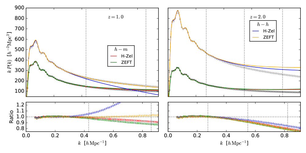
Figure 8: As for Fig. 3, but for the simpler models Halo-Zeldovich (H-Zel) and ZEFT, defined using Eq. (B.1). The diamonds are for the halo auto-spectra while the circles are for the halo-matter cross-spectra (we have omitted the matter auto-correlation). The lower panels now show the ratio of the N-body to both the theories on an expanded $y$-axis scale for both.

The two simpler models are based upon the “ZEFT” model of Ref. [50] and the “Halo-Zeldovich” model of Ref. [94, 95], both modified to include biased tracers as in Ref. [45, 96]. These models have the same number of free parameters as our CLEFT model and the same flexible bias model, while requiring only 1D integrals of the linear theory power spectrum so they can be evaluated very quickly. While not as accurate as the CLEFT model, they provide an adequate fit to our N-body simulations over the whole range of redshift (even at lower $z$) which may be sufficient for the next few years.

The power spectra of the models is of the same form as Eq. (2.8) but the individual contributions, $f_{x}$, contain only tree-level terms. For the Halo-Zeldovich model there is a constant term added whose amplitude forms a free parameter. Explicitly

$$P_{HZ} = 4\pi\int q^{2}\,dq\ e^{-(1/2)k^{2}(X_{L}+Y_{L})}\left\{\vphantom{\int}\right.$$ (B.1)

$$\left[1+b_{1}^{2}\left(\xi_{L}-k^{2}U_{L}^{2}\right)-b_{2}\left(k^{2}U_{L}^{2}\right)+\frac{b_{2}^{2}}{2}\xi_{L}^{2}\right]j_{0}(kq)$$

$$+ \sum_{n=1}^{\infty}\left[1-2b_{1}\frac{q\,U_{L}}{Y_{L}}+b_{1}^{2}\left(\xi_{L}+\left[\frac{2n}{Y_{L}}-k^{2}\right]U_{L}^{2}\right)+b_{2}\left(\frac{2n}{Y_{L}}-k^{2}\right)U_{L}^{2}\right.$$

$$\left.\left.-2b_{1}b_{2}\frac{q\,U_{L}\,\xi_{L}}{Y_{L}}+\frac{b_{2}^{2}}{2}\xi_{L}^{2}\right]\left(\frac{k\,Y_{L}}{q}\right)^{n}j_{n}(kq)\right\}+1-{\rm halo}$$

where the integral over $q$ can be done efficiently using fast Fourier transforms [97, 98] or other methods [99, 100] and we can take the 1-halo term as a constant. For completeness

$$\xi_{L}(q) = \frac{1}{2\pi^{2}}\int_{0}^{\infty}dk\ P_{L}(k)\left[k^{2}\,j_{0}(kq)\right]$$ (B.2)

$$X_{L}(q) = \frac{1}{2\pi^{2}}\int_{0}^{\infty}dk\ P_{L}(k)\left[\frac{2}{3}-2\frac{j_{1}(kq)}{kq}\right]$$ (B.3)

$$Y_{L}(q) = \frac{1}{2\pi^{2}}\int_{0}^{\infty}dk\ P_{L}(k)\left[-2j_{0}(kq)+6\frac{j_{1}(kq)}{kq}\right]$$ (B.4)

$$U_{L}(q) = \frac{1}{2\pi^{2}}\int_{0}^{\infty}dk\ P_{L}(k)\left[-k\,j_{1}(kq)\right]$$ (B.5)

We have omitted the dependence upon $b_{s^{2}}$ and $b_{\nabla^{2}}$ as unceccessary for this level of approximation. As in the main text, the auto-correlation contains all of the terms while the cross-correlation with the matter contains only terms linear in $b_{1}$ and $b_{2}$ (divided by 2).

The alternative is the “ZEFT” model. In this model the 1-halo term is replaced by $\alpha k^{2}P_{\rm Z}$, and thus has the same number of free parameters. Note that this substitution requires no additional calculation, since $P_{\rm Z}$ is already computed as part of $P_{HZ}$. Fig. 8 shows the performance of the models at $z=1$ and $2$ compared to our $10^{12}\,h^{-1}M_{\odot}$ halo sample. We find the performance of the two models similar, with the ZEFT model performing slightly better, especially at lower redshifts. Both the models agree to within $1\%$ with the N-body results out to $k=0.2\,h\,$Mpc^-1 and within $5\%$ to $k=0.4\,h\,$Mpc^-1 at $z=1$ and $2$. Neither model performs as well as CLEFT, even at high redshift, because even at $z=3$ the 1-loop contributions to both, matter and the bias terms are not negligible, and act to improve agreement with the N-body.

Of course it is possible to further improve the performance of these models by introducing more free parameters or by combining the $\alpha k^{2}P_{\rm Z}$ and 1-halo terms. We found this gave negligible improvement. The 1-halo term can be replaced by a power series in $k$, or a Padé term. We have experimented with terms of the form $(k\Sigma)^{2}/[1+(k\Sigma)^{2}]$ but did not find very dramatic improvements. Further progress would obviously require more degrees of freedom in the 1-halo term.

References

- [1] A. Lewis and A. Challinor, Weak gravitational lensing of the CMB, PhysRep 429 (June, 2006) 1–65, [astro-ph/0601594].
- [2] D. Hanson, A. Challinor, and A. Lewis, Weak lensing of the CMB, General Relativity and Gravitation 42 (Sept., 2010) 2197–2218, [arXiv:0911.0612].
- [3] K. M. Smith, O. Zahn, and O. Doré, Detection of gravitational lensing in the cosmic microwave background, PRD 76 (Aug., 2007) 043510, [arXiv:0705.3980].
- [4] C. M. Hirata, S. Ho, N. Padmanabhan, U. Seljak, and N. A. Bahcall, Correlation of CMB with large-scale structure. II. Weak lensing, PRD 78 (Aug., 2008) 043520, [arXiv:0801.0644].
- [5] A. van Engelen, R. Keisler, O. Zahn, K. A. Aird, B. A. Benson, L. E. Bleem, J. E. Carlstrom, C. L. Chang, H. M. Cho, T. M. Crawford, A. T. Crites, T. de Haan, M. A. Dobbs, J. Dudley, E. M. George, N. W. Halverson, G. P. Holder, W. L. Holzapfel, S. Hoover, Z. Hou, J. D. Hrubes, M. Joy, L. Knox, A. T. Lee, E. M. Leitch, M. Lueker, D. Luong-Van, J. J. McMahon, J. Mehl, S. S. Meyer, M. Millea, J. J. Mohr, T. E. Montroy, T. Natoli, S. Padin, T. Plagge, C. Pryke, C. L. Reichardt, J. E. Ruhl, J. T. Sayre, K. K. Schaffer, L. Shaw, E. Shirokoff, H. G. Spieler, Z. Staniszewski, A. A. Stark, K. Story, K. Vanderlinde, J. D. Vieira, and R. Williamson, A Measurement of Gravitational Lensing of the Microwave Background Using South Pole Telescope Data, ApJ 756 (Sept., 2012) 142, [arXiv:1202.0546].
- [6] P. A. R. Ade, Y. Akiba, A. E. Anthony, K. Arnold, M. Atlas, D. Barron, D. Boettger, J. Borrill, S. Chapman, Y. Chinone, M. Dobbs, T. Elleflot, J. Errard, G. Fabbian, C. Feng, D. Flanigan, A. Gilbert, W. Grainger, N. W. Halverson, M. Hasegawa, K. Hattori, M. Hazumi, W. L. Holzapfel, Y. Hori, J. Howard, P. Hyland, Y. Inoue, G. C. Jaehnig, A. Jaffe, B. Keating, Z. Kermish, R. Keskitalo, T. Kisner, M. Le Jeune, A. T. Lee, E. Linder, E. M. Leitch, M. Lungu, F. Matsuda, T. Matsumura, X. Meng, N. J. Miller, H. Morii, S. Moyerman, M. J. Myers, M. Navaroli, H. Nishino, H. Paar, J. Peloton, E. Quealy, G. Rebeiz, C. L. Reichardt, P. L. Richards, C. Ross, I. Schanning, D. E. Schenck, B. Sherwin, A. Shimizu, C. Shimmin, M. Shimon, P. Siritanasak, G. Smecher, H. Spieler, N. Stebor, B. Steinbach, R. Stompor, A. Suzuki, S. Takakura, T. Tomaru, B. Wilson, A. Yadav, O. Zahn, and Polarbear Collaboration, Measurement of the Cosmic Microwave Background Polarization Lensing Power Spectrum with the POLARBEAR Experiment, Physical Review Letters 113 (July, 2014) 021301, [arXiv:1312.6646].
- [7] A. van Engelen, B. D. Sherwin, N. Sehgal, G. E. Addison, R. Allison, N. Battaglia, F. de Bernardis, J. R. Bond, E. Calabrese, K. Coughlin, D. Crichton, R. Datta, M. J. Devlin, J. Dunkley, R. Dünner, P. Gallardo, E. Grace, M. Gralla, A. Hajian, M. Hasselfield, S. Henderson, J. C. Hill, M. Hilton, A. D. Hincks, R. Hlozek, K. M. Huffenberger, J. P. Hughes, B. Koopman, A. Kosowsky, T. Louis, M. Lungu, M. Madhavacheril, L. Maurin, J. McMahon, K. Moodley, C. Munson, S. Naess, F. Nati, L. Newburgh, M. D. Niemack, M. R. Nolta, L. A. Page, C. Pappas, B. Partridge, B. L. Schmitt, J. L. Sievers, S. Simon, D. N. Spergel, S. T. Staggs, E. R. Switzer, J. T. Ward, and E. J. Wollack, The Atacama Cosmology Telescope: Lensing of CMB Temperature and Polarization Derived from Cosmic Infrared Background Cross-correlation, ApJ 808 (July, 2015) 7, [arXiv:1412.0626].
- [8] Planck Collaboration, P. A. R. Ade, N. Aghanim, C. Armitage-Caplan, M. Arnaud, M. Ashdown, F. Atrio-Barandela, J. Aumont, C. Baccigalupi, A. J. Banday, and et al., Planck 2013 results. XVII. Gravitational lensing by large-scale structure, A&A 571 (Nov., 2014) A17, [arXiv:1303.5077].
- [9] Planck Collaboration, P. A. R. Ade, N. Aghanim, M. Arnaud, M. Ashdown, J. Aumont, C. Baccigalupi, A. J. Banday, R. B. Barreiro, J. G. Bartlett, and et al., Planck 2015 results. XV. Gravitational lensing, A&A 594 (Sept., 2016) A15, [arXiv:1502.01591].
- [10] F. De Bernardis, J. R. Stevens, M. Hasselfield, D. Alonso, J. R. Bond, E. Calabrese, S. K. Choi, K. T. Crowley, M. Devlin, J. Dunkley, P. A. Gallardo, S. W. Henderson, M. Hilton, R. Hlozek, S. P. Ho, K. Huffenberger, B. J. Koopman, A. Kosowsky, T. Louis, M. S. Madhavacheril, J. McMahon, S. Næss, F. Nati, L. Newburgh, M. D. Niemack, L. A. Page, M. Salatino, A. Schillaci, B. L. Schmitt, N. Sehgal, J. L. Sievers, S. M. Simon, D. N. Spergel, S. T. Staggs, A. van Engelen, E. M. Vavagiakis, and E. J. Wollack, Survey strategy optimization for the Atacama Cosmology Telescope, in Observatory Operations: Strategies, Processes, and Systems VI, vol. 9910 of SPIE, p. 991014, July, 2016. arXiv:1607.02120.
- [11] A. Suzuki, P. Ade, Y. Akiba, C. Aleman, K. Arnold, C. Baccigalupi, B. Barch, D. Barron, A. Bender, D. Boettger, J. Borrill, S. Chapman, Y. Chinone, A. Cukierman, M. Dobbs, A. Ducout, R. Dunner, T. Elleflot, J. Errard, G. Fabbian, S. Feeney, C. Feng, T. Fujino, G. Fuller, A. Gilbert, N. Goeckner-Wald, J. Groh, T. D. Haan, G. Hall, N. Halverson, T. Hamada, M. Hasegawa, K. Hattori, M. Hazumi, C. Hill, W. Holzapfel, Y. Hori, L. Howe, Y. Inoue, F. Irie, G. Jaehnig, A. Jaffe, O. Jeong, N. Katayama, J. Kaufman, K. Kazemzadeh, B. Keating, Z. Kermish, R. Keskitalo, T. Kisner, A. Kusaka, M. L. Jeune, A. Lee, D. Leon, E. Linder, L. Lowry, F. Matsuda, T. Matsumura, N. Miller, K. Mizukami, J. Montgomery, M. Navaroli, H. Nishino, J. Peloton, D. Poletti, G. Puglisi, G. Rebeiz, C. Raum, C. Reichardt, P. Richards, C. Ross, K. Rotermund, Y. Segawa, B. Sherwin, I. Shirley, P. Siritanasak, N. Stebor, R. Stompor, J. Suzuki, O. Tajima, S. Takada, S. Takakura, S. Takatori, A. Tikhomirov, T. Tomaru, B. Westbrook, N. Whitehorn, T. Yamashita, A. Zahn, and O. Zahn, The Polarbear-2 and the Simons Array Experiments, Journal of Low Temperature Physics 184 (Aug., 2016) 805–810, [arXiv:1512.07299].
- [12] K. N. Abazajian, P. Adshead, Z. Ahmed, S. W. Allen, D. Alonso, K. S. Arnold, C. Baccigalupi, J. G. Bartlett, N. Battaglia, B. A. Benson, C. A. Bischoff, J. Borrill, V. Buza, E. Calabrese, R. Caldwell, J. E. Carlstrom, C. L. Chang, T. M. Crawford, F.-Y. Cyr-Racine, F. De Bernardis, T. de Haan, S. di Serego Alighieri, J. Dunkley, C. Dvorkin, J. Errard, G. Fabbian, S. Feeney, S. Ferraro, J. P. Filippini, R. Flauger, G. M. Fuller, V. Gluscevic, D. Green, D. Grin, E. Grohs, J. W. Henning, J. C. Hill, R. Hlozek, G. Holder, W. Holzapfel, W. Hu, K. M. Huffenberger, R. Keskitalo, L. Knox, A. Kosowsky, J. Kovac, E. D. Kovetz, C.-L. Kuo, A. Kusaka, M. Le Jeune, A. T. Lee, M. Lilley, M. Loverde, M. S. Madhavacheril, A. Mantz, D. J. E. Marsh, J. McMahon, P. D. Meerburg, J. Meyers, A. D. Miller, J. B. Munoz, H. N. Nguyen, M. D. Niemack, M. Peloso, J. Peloton, L. Pogosian, C. Pryke, M. Raveri, C. L. Reichardt, G. Rocha, A. Rotti, E. Schaan, M. M. Schmittfull, D. Scott, N. Sehgal, S. Shandera, B. D. Sherwin, T. L. Smith, L. Sorbo, G. D. Starkman, K. T. Story, A. van Engelen, J. D. Vieira, S. Watson, N. Whitehorn, and W. L. Kimmy Wu, CMB-S4 Science Book, First Edition, ArXiv e-prints (Oct., 2016) [arXiv:1610.02743].
- [13] E. Baxter, J. Clampitt, T. Giannantonio, S. Dodelson, B. Jain, D. Huterer, L. Bleem, T. Crawford, G. Efstathiou, P. Fosalba, D. Kirk, J. Kwan, C. Sánchez, K. Story, M. A. Troxel, T. M. C. Abbott, F. B. Abdalla, R. Armstrong, A. Benoit-Lévy, B. Benson, G. M. Bernstein, R. A. Bernstein, E. Bertin, D. Brooks, J. Carlstrom, A. C. Rosell, M. Carrasco Kind, J. Carretero, R. Chown, M. Crocce, C. E. Cunha, L. N. da Costa, S. Desai, H. T. Diehl, J. P. Dietrich, P. Doel, A. E. Evrard, A. Fausti Neto, B. Flaugher, J. Frieman, D. Gruen, R. A. Gruendl, G. Gutierrez, T. de Haan, G. Holder, K. Honscheid, Z. Hou, D. J. James, K. Kuehn, N. Kuropatkin, M. Lima, M. March, J. L. Marshall, P. Martini, P. Melchior, C. J. Miller, R. Miquel, J. J. Mohr, B. Nord, Y. Omori, A. A. Plazas, C. Reichardt, A. K. Romer, E. S. Rykoff, E. Sanchez, I. Sevilla-Noarbe, E. Sheldon, R. C. Smith, M. Soares-Santos, F. Sobreira, E. Suchyta, A. Stark, M. E. C. Swanson, G. Tarle, D. Thomas, A. R. Walker, and R. H. Wechsler, Joint measurement of lensing-galaxy correlations using SPT and DES SV data, MNRAS 461 (Oct., 2016) 4099–4114, [arXiv:1602.07384].
- [14] A. Vallinotto, Using Cosmic Microwave Background Lensing to Constrain the Multiplicative Bias of Cosmic Shear, ApJ 759 (Nov., 2012) 32, [arXiv:1110.5339].
- [15] A. Vallinotto, The Synergy between the Dark Energy Survey and the South Pole Telescope, ApJ 778 (Dec., 2013) 108, [arXiv:1304.3474].
- [16] S. Das, J. Errard, and D. Spergel, Can CMB Lensing Help Cosmic Shear Surveys?, ArXiv e-prints (Nov., 2013) [arXiv:1311.2338].
- [17] J. Liu, A. Ortiz-Vazquez, and J. C. Hill, Constraining multiplicative bias in CFHTLenS weak lensing shear data, PRD 93 (May, 2016) 103508, [arXiv:1601.05720].
- [18] S. Singh, R. Mandelbaum, and J. R. Brownstein, Cross-correlating Planck CMB lensing with SDSS: lensing-lensing and galaxy-lensing cross-correlations, MNRAS 464 (Jan., 2017) 2120–2138, [arXiv:1606.08841].
- [19] E. Schaan, E. Krause, T. Eifler, O. Doré, H. Miyatake, J. Rhodes, and D. N. Spergel, Looking through the same lens: shear calibration for LSST, Euclid and WFIRST with stage 4 CMB lensing, ArXiv e-prints (July, 2016) [arXiv:1607.01761].
- [20] L. E. Bleem, A. van Engelen, G. P. Holder, K. A. Aird, R. Armstrong, M. L. N. Ashby, M. R. Becker, B. A. Benson, T. Biesiadzinski, M. Brodwin, M. T. Busha, J. E. Carlstrom, C. L. Chang, H. M. Cho, T. M. Crawford, A. T. Crites, T. de Haan, S. Desai, M. A. Dobbs, O. Doré, J. Dudley, J. E. Geach, E. M. George, M. D. Gladders, A. H. Gonzalez, N. W. Halverson, N. Harrington, F. W. High, B. P. Holden, W. L. Holzapfel, S. Hoover, J. D. Hrubes, M. Joy, R. Keisler, L. Knox, A. T. Lee, E. M. Leitch, M. Lueker, D. Luong-Van, D. P. Marrone, J. Martinez-Manso, J. J. McMahon, J. Mehl, S. S. Meyer, J. J. Mohr, T. E. Montroy, T. Natoli, S. Padin, T. Plagge, C. Pryke, C. L. Reichardt, A. Rest, J. E. Ruhl, B. R. Saliwanchik, J. T. Sayre, K. K. Schaffer, L. Shaw, E. Shirokoff, H. G. Spieler, B. Stalder, S. A. Stanford, Z. Staniszewski, A. A. Stark, D. Stern, K. Story, A. Vallinotto, K. Vanderlinde, J. D. Vieira, R. H. Wechsler, R. Williamson, and O. Zahn, A Measurement of the Correlation of Galaxy Surveys with CMB Lensing Convergence Maps from the South Pole Telescope, ApJL 753 (July, 2012) L9, [arXiv:1203.4808].
- [21] B. D. Sherwin, S. Das, A. Hajian, G. Addison, J. R. Bond, D. Crichton, M. J. Devlin, J. Dunkley, M. B. Gralla, M. Halpern, J. C. Hill, A. D. Hincks, J. P. Hughes, K. Huffenberger, R. Hlozek, A. Kosowsky, T. Louis, T. A. Marriage, D. Marsden, F. Menanteau, K. Moodley, M. D. Niemack, L. A. Page, E. D. Reese, N. Sehgal, J. Sievers, C. Sifón, D. N. Spergel, S. T. Staggs, E. R. Switzer, and E. Wollack, The Atacama Cosmology Telescope: Cross-correlation of cosmic microwave background lensing and quasars, PRD 86 (Oct., 2012) 083006, [arXiv:1207.4543].
- [22] J. E. Geach, R. C. Hickox, L. E. Bleem, M. Brodwin, G. P. Holder, K. A. Aird, B. A. Benson, S. Bhattacharya, J. E. Carlstrom, C. L. Chang, H.-M. Cho, T. M. Crawford, A. T. Crites, T. de Haan, M. A. Dobbs, J. Dudley, E. M. George, K. N. Hainline, N. W. Halverson, W. L. Holzapfel, S. Hoover, Z. Hou, J. D. Hrubes, R. Keisler, L. Knox, A. T. Lee, E. M. Leitch, M. Lueker, D. Luong-Van, D. P. Marrone, J. J. McMahon, J. Mehl, S. S. Meyer, M. Millea, J. J. Mohr, T. E. Montroy, A. D. Myers, S. Padin, T. Plagge, C. Pryke, C. L. Reichardt, J. E. Ruhl, J. T. Sayre, K. K. Schaffer, L. Shaw, E. Shirokoff, H. G. Spieler, Z. Staniszewski, A. A. Stark, K. T. Story, A. van Engelen, K. Vanderlinde, J. D. Vieira, R. Williamson, and O. Zahn, A Direct Measurement of the Linear Bias of Mid-infrared-selected Quasars at z of 1 Using Cosmic Microwave Background Lensing, ApJL 776 (Oct., 2013) L41, [arXiv:1307.1706].
- [23] Y. Omori and G. Holder, Cross-Correlation of CFHTLenS Galaxy Number Density and Planck CMB Lensing, ArXiv e-prints (Feb., 2015) [arXiv:1502.03405].
- [24] S. Ferraro, B. D. Sherwin, and D. N. Spergel, WISE measurement of the integrated Sachs-Wolfe effect, PRD 91 (Apr., 2015) 083533, [arXiv:1401.1193].
- [25] M. A. DiPompeo, A. D. Myers, R. C. Hickox, J. E. Geach, G. Holder, K. N. Hainline, and S. W. Hall, Weighing obscured and unobscured quasar hosts with the cosmic microwave background, MNRAS 446 (Feb., 2015) 3492–3501, [arXiv:1411.0527].
- [26] M. A. DiPompeo, R. C. Hickox, and A. D. Myers, Updated measurements of the dark matter halo masses of obscured quasars with improved WISE and Planck data, MNRAS 456 (Feb., 2016) 924–942, [arXiv:1511.04469].
- [27] R. Allison, S. N. Lindsay, B. D. Sherwin, F. de Bernardis, J. R. Bond, E. Calabrese, M. J. Devlin, J. Dunkley, P. Gallardo, S. Henderson, A. D. Hincks, R. Hlozek, M. Jarvis, A. Kosowsky, T. Louis, M. Madhavacheril, J. McMahon, K. Moodley, S. Naess, L. Newburgh, M. D. Niemack, L. A. Page, B. Partridge, N. Sehgal, D. N. Spergel, S. T. Staggs, A. van Engelen, and E. J. Wollack, The Atacama Cosmology Telescope: measuring radio galaxy bias through cross-correlation with lensing, MNRAS 451 (July, 2015) 849–858, [arXiv:1502.06456].
- [28] F. Bianchini, P. Bielewicz, A. Lapi, J. Gonzalez-Nuevo, C. Baccigalupi, G. de Zotti, L. Danese, N. Bourne, A. Cooray, L. Dunne, S. Dye, S. Eales, R. Ivison, S. Maddox, M. Negrello, D. Scott, M. W. L. Smith, and E. Valiante, Cross-correlation between the CMB Lensing Potential Measured by Planck and High-z Submillimeter Galaxies Detected by the Herschel-Atlas Survey, ApJ 802 (Mar., 2015) 64, [arXiv:1410.4502].
- [29] A. R. Pullen, S. Alam, S. He, and S. Ho, Constraining gravity at the largest scales through CMB lensing and galaxy velocities, MNRAS 460 (Aug., 2016) 4098–4108, [arXiv:1511.04457].
- [30] T. Giannantonio, P. Fosalba, R. Cawthon, Y. Omori, M. Crocce, F. Elsner, B. Leistedt, S. Dodelson, A. Benoit-Lévy, E. Gaztañaga, G. Holder, H. V. Peiris, W. J. Percival, D. Kirk, A. H. Bauer, B. A. Benson, G. M. Bernstein, J. Carretero, T. M. Crawford, R. Crittenden, D. Huterer, B. Jain, E. Krause, C. L. Reichardt, A. J. Ross, G. Simard, B. Soergel, A. Stark, K. T. Story, J. D. Vieira, J. Weller, T. Abbott, F. B. Abdalla, S. Allam, R. Armstrong, M. Banerji, R. A. Bernstein, E. Bertin, D. Brooks, E. Buckley-Geer, D. L. Burke, D. Capozzi, J. E. Carlstrom, A. Carnero Rosell, M. Carrasco Kind, F. J. Castander, C. L. Chang, C. E. Cunha, L. N. da Costa, C. B. D’Andrea, D. L. DePoy, S. Desai, H. T. Diehl, J. P. Dietrich, P. Doel, T. F. Eifler, A. E. Evrard, A. F. Neto, E. Fernandez, D. A. Finley, B. Flaugher, J. Frieman, D. Gerdes, D. Gruen, R. A. Gruendl, G. Gutierrez, W. L. Holzapfel, K. Honscheid, D. J. James, K. Kuehn, N. Kuropatkin, O. Lahav, T. S. Li, M. Lima, M. March, J. L. Marshall, P. Martini, P. Melchior, R. Miquel, J. J. Mohr, R. C. Nichol, B. Nord, R. Ogando, A. A. Plazas, A. K. Romer, A. Roodman, E. S. Rykoff, M. Sako, B. R. Saliwanchik, E. Sanchez, M. Schubnell, I. Sevilla-Noarbe, R. C. Smith, M. Soares-Santos, F. Sobreira, E. Suchyta, M. E. C. Swanson, G. Tarle, J. Thaler, D. Thomas, V. Vikram, A. R. Walker, R. H. Wechsler, and J. Zuntz, CMB lensing tomography with the DES Science Verification galaxies, MNRAS 456 (Mar., 2016) 3213–3244, [arXiv:1507.05551].
- [31] J. Liu and J. C. Hill, Cross-correlation of Planck CMB lensing and CFHTLenS galaxy weak lensing maps, PRD 92 (Sept., 2015) 063517, [arXiv:1504.05598].
- [32] H. Miyatake, M. S. Madhavacheril, N. Sehgal, A. Slosar, D. N. Spergel, B. Sherwin, and A. van Engelen, Measurement of a Cosmographic Distance Ratio with Galaxy and CMB Lensing, ArXiv e-prints (May, 2016) [arXiv:1605.05337].
- [33] S. Singh, R. Mandelbaum, and J. R. Brownstein, Cross-correlating Planck CMB lensing with SDSS: lensing-lensing and galaxy-lensing cross-correlations, MNRAS 464 (Jan., 2017) 2120–2138, [arXiv:1606.08841].
- [34] J. Harnois-Déraps, T. Tröster, A. Hojjati, L. van Waerbeke, M. Asgari, A. Choi, T. Erben, C. Heymans, H. Hildebrandt, T. D. Kitching, L. Miller, R. Nakajima, M. Viola, S. Arnouts, J. Coupon, and T. Moutard, CFHTLenS and RCSLenS cross-correlation with Planck lensing detected in fourier and configuration space, MNRAS 460 (July, 2016) 434–457, [arXiv:1603.07723].
- [35] J. Harnois-Déraps, T. Tröster, N. E. Chisari, C. Heymans, L. van Waerbeke, M. Asgari, M. Bilicki, A. Choi, H. Hildebrandt, H. Hoekstra, S. Joudaki, K. Kuijken, J. Merten, L. Miller, N. Robertson, P. Schneider, and M. Viola, KiDS-450: Tomographic Cross-Correlation of Galaxy Shear with it Planck Lensing, ArXiv e-prints (Mar., 2017) [arXiv:1703.03383].
- [36] C. Doux, E. Schaan, E. Aubourg, K. Ganga, K.-G. Lee, D. N. Spergel, and J. Tréguer, First detection of cosmic microwave background lensing and Lyman- forest bispectrum, PRD 94 (Nov., 2016) 103506, [arXiv:1607.03625].
- [37] Y. Omori, R. Chown, G. Simard, K. T. Story, K. Aylor, E. J. Baxter, B. A. Benson, L. E. Bleem, J. E. Carlstrom, C. L. Chang, H. Cho, T. M. Crawford, A. T. Crites, T. de Haan, M. A. Dobbs, W. B. Everett, E. M. George, N. W. Halverson, N. L. Harrington, G. P. Holder, Z. Hou, W. L. Holzapfel, J. D. Hrubes, L. Knox, A. T. Lee, E. M. Leitch, D. Luong-Van, A. Manzotti, D. P. Marrone, J. J. McMahon, S. S. Meyer, L. M. Mocanu, J. J. Mohr, T. Natoli, S. Padin, C. Pryke, C. L. Reichardt, J. E. Ruhl, J. T. Sayre, K. K. Schaffer, E. Shirokoff, Z. Staniszewski, A. A. Stark, K. Vanderlinde, J. D. Vieira, R. Williamson, and O. Zahn, A 2500 square-degree CMB lensing map from combined South Pole Telescope and Planck data, ArXiv e-prints (May, 2017) [arXiv:1705.00743].
- [38] N. Fornengo, L. Perotto, M. Regis, and S. Camera, Evidence of Cross-correlation between the CMB Lensing and the -Ray Sky, ApJL 802 (Mar., 2015) L1, [arXiv:1410.4997].
- [39] C. Feng, A. Cooray, and B. Keating, Planck Lensing and Cosmic Infrared Background Cross-correlation with Fermi-LAT: Tracing Dark Matter Signals in the Gamma-ray Background, ApJ 836 (Feb., 2017) 127, [arXiv:1608.04351].
- [40] Z. Vlah, E. Castorina, and M. White, The Gaussian streaming model and convolution Lagrangian effective field theory, JCAP 12 (Dec., 2016) 007, [arXiv:1609.02908].
- [41] T. Buchert, A class of solutions in Newtonian cosmology and the pancake theory, A&A 223 (Oct., 1989) 9–24.
- [42] F. Moutarde, J.-M. Alimi, F. R. Bouchet, R. Pellat, and A. Ramani, Precollapse scale invariance in gravitational instability, ApJ 382 (Dec., 1991) 377–381.
- [43] E. Hivon, F. R. Bouchet, S. Colombi, and R. Juszkiewicz, Redshift distortions of clustering: a Lagrangian approach., A&A 298 (June, 1995) 643, [astro-ph/9407049].
- [44] T. Matsubara, Resumming cosmological perturbations via the Lagrangian picture: One-loop results in real space and in redshift space, PRD 77 (Mar., 2008) 063530, [arXiv:0711.2521].
- [45] T. Matsubara, Nonlinear perturbation theory with halo bias and redshift-space distortions via the Lagrangian picture, PRD 78 (Oct., 2008) 083519, [arXiv:0807.1733].
- [46] J. Carlson, B. Reid, and M. White, Convolution Lagrangian perturbation theory for biased tracers, MNRAS 429 (Feb., 2013) 1674–1685, [arXiv:1209.0780].
- [47] R. A. Porto, L. Senatore, and M. Zaldarriaga, The Lagrangian-space Effective Field Theory of large scale structures, JCAP 5 (May, 2014) 022, [arXiv:1311.2168].
- [48] M. McQuinn and M. White, Cosmological perturbation theory in 1+1 dimensions, ArXiv e-prints (Feb., 2015) [arXiv:1502.07389].
- [49] Z. Vlah, U. Seljak, and T. Baldauf, Lagrangian perturbation theory at one loop order: Successes, failu res, and improvements, PRD 91 (Jan., 2015) 023508, [arXiv:1410.1617].
- [50] Z. Vlah, M. White, and A. Aviles, A Lagrangian effective field theory, JCAP 9 (Sept., 2015) 014, [arXiv:1506.05264].
- [51] M. Loverde and N. Afshordi, Extended Limber approximation, PRD 78 (Dec., 2008) 123506, [arXiv:0809.5112].
- [52] J. R. Shaw and A. Lewis, Nonlinear redshift-space power spectra, PRD 78 (Nov., 2008) 103512, [arXiv:0808.1724].
- [53] S. Foreman and L. Senatore, The EFT of Large Scale Structures at all redshifts: analytical predictions for lensing, JCAP 4 (Apr., 2016) 033, [arXiv:1503.01775].
- [54] D. Blas, J. Lesgourgues, and T. Tram, The Cosmic Linear Anisotropy Solving System (CLASS). Part II: Approximation schemes, JCAP 7 (July, 2011) 034, [arXiv:1104.2933].
- [55] LSST Science Collaboration, P. A. Abell, J. Allison, S. F. Anderson, J. R. Andrew, J. R. P. Angel, L. Armus, D. Arnett, S. J. Asztalos, T. S. Axelrod, and et al., LSST Science Book, Version 2.0, ArXiv e-prints (Dec., 2009) [arXiv:0912.0201].
- [56] C. C. Steidel, K. L. Adelberger, A. E. Shapley, M. Pettini, M. Dickinson, and M. Giavalisco, Lyman Break Galaxies at Redshift : Survey Description and Full Data Set, ApJ 592 (Aug., 2003) 728–754, [astro-ph/0305378].
- [57] K. L. Adelberger, C. C. Steidel, M. Pettini, A. E. Shapley, N. A. Reddy, and D. K. Erb, The Spatial Clustering of Star-forming Galaxies at Redshifts , ApJ 619 (Feb., 2005) 697–713, [astro-ph/0410165].
- [58] N. A. Reddy, C. C. Steidel, M. Pettini, K. L. Adelberger, A. E. Shapley, D. K. Erb, and M. Dickinson, Multiwavelength Constraints on the Cosmic Star Formation History from Spectroscopy: The Rest-Frame Ultraviolet, H, and Infrared Luminosity Functions at Redshifts , ApJS 175 (Mar., 2008) 48–85, [arXiv:0706.4091].
- [59] V. Böhm, M. Schmittfull, and B. D. Sherwin, Bias to CMB lensing measurements from the bispectrum of large-scale structure, PRD 94 (Aug., 2016) 043519, [arXiv:1605.01392].
- [60] A. Lewis and G. Pratten, Effect of lensing non-Gaussianity on the CMB power spectra, JCAP 12 (Dec., 2016) 003, [arXiv:1608.01263].
- [61] A. Amblard, C. Vale, and M. White, Weak lensing of the CMB by large-scale structure, New Astronomy 9 (Oct., 2004) 687–704, [astro-ph/0403075].
- [62] S. Ferraro and J. C. Hill, Bias to CMB Lensing Reconstruction from Temperature Anisotropies due to Large-Scale Galaxy Motions, ArXiv e-prints (May, 2017) [arXiv:1705.06751].
- [63] F. Bernardeau, S. Colombi, E. Gaztañaga, and R. Scoccimarro, Large-scale structure of the Universe and cosmological perturbation theory, PhysRep 367 (Sept., 2002) 1–248, [astro-ph/0112551].
- [64] R. Takahashi, Third-Order Density Perturbation and One-Loop Power Spectrum in Dark-Energy-Dominated Universe, Progress of Theoretical Physics 120 (Sept., 2008) 549–559, [arXiv:0806.1437].
- [65] M. Fasiello and Z. Vlah, Non-linear Fields in Generalized Cosmologies, ArXiv e-prints (Apr., 2016) [arXiv:1604.04612].
- [66] V. Desjacques, D. Jeong, and F. Schmidt, Large-Scale Galaxy Bias, ArXiv e-prints (Nov., 2016) [arXiv:1611.09787].
- [67] W. H. Press and P. Schechter, Formation of Galaxies and Clusters of Galaxies by Self-Similar Gravitational Condensation, ApJ 187 (Feb., 1974) 425–438.
- [68] T. Lazeyras, M. Musso, and V. Desjacques, Lagrangian bias of generic large-scale structure tracers, PRD 93 (Mar., 2016) 063007, [arXiv:1512.05283].
- [69] E. Castorina, A. Paranjape, O. Hahn, and R. K. Sheth, Excursion set peaks: the role of shear, ArXiv e-prints (Nov., 2016) [arXiv:1611.03619].
- [70] C. Modi, E. Castorina, and U. Seljak, Halo bias in Lagrangian Space: Estimators and theoretical predictions, ArXiv e-prints (Dec., 2016) [arXiv:1612.01621].
- [71] M. White, The Mass Function, ApJS 143 (Dec., 2002) 241–255, [astro-ph/0207185].
- [72] B. A. Reid, H.-J. Seo, A. Leauthaud, J. L. Tinker, and M. White, A 2.5 per cent measurement of the growth rate from small-scale redshift space clustering of SDSS-III CMASS galaxies, MNRAS 444 (Oct., 2014) 476–502, [arXiv:1404.3742].
- [73] M. White, B. Reid, C.-H. Chuang, J. L. Tinker, C. K. McBride, F. Prada, and L. Samushia, Tests of redshift-space distortions models in configuration space for the analysis of the BOSS final data release, MNRAS 447 (Feb., 2015) 234–245, [arXiv:1408.5435].
- [74] R. Takahashi, M. Sato, T. Nishimichi, A. Taruya, and M. Oguri, Revising the Halofit Model for the Nonlinear Matter Power Spectrum, ApJ 761 (Dec., 2012) 152, [arXiv:1208.2701].
- [75] E. Lawrence, K. Heitmann, J. Kwan, A. Upadhye, D. Bingham, S. Habib, D. Higdon, A. Pope, H. Finkel, and N. Frontiere, The Mira-Titan Universe II: Matter Power Spectrum Emulation, ArXiv e-prints (May, 2017) [arXiv:1705.03388].
- [76] B. A. Reid, L. Samushia, M. White, W. J. Percival, M. Manera, N. Padmanabhan, A. J. Ross, A. G. Sánchez, S. Bailey, D. Bizyaev, A. S. Bolton, H. Brewington, J. Brinkmann, J. R. Brownstein, A. J. Cuesta, D. J. Eisenstein, J. E. Gunn, K. Honscheid, E. Malanushenko, V. Malanushenko, C. Maraston, C. K. McBride, D. Muna, R. C. Nichol, D. Oravetz, K. Pan, R. de Putter, N. A. Roe, N. P. Ross, D. J. Schlegel, D. P. Schneider, H.-J. Seo, A. Shelden, E. S. Sheldon, A. Simmons, R. A. Skibba, S. Snedden, M. E. C. Swanson, D. Thomas, J. Tinker, R. Tojeiro, L. Verde, D. A. Wake, B. A. Weaver, D. H. Weinberg, I. Zehavi, and G.-B. Zhao, The clustering of galaxies in the SDSS-III Baryon Oscillation Spectroscopic Survey: measurements of the growth of structure and expansion rate at z = 0.57 from anisotropic clustering, MNRAS 426 (Nov., 2012) 2719–2737, [arXiv:1203.6641].
- [77] D. Foreman-Mackey, D. W. Hogg, D. Lang, and J. Goodman, emcee: The MCMC Hammer, Publ. Astron. Soc. Pac. 125 (Mar., 2013) 306, [arXiv:1202.3665].
- [78] M. McQuinn and M. White, On using angular cross-correlations to determine source redshift distributions, MNRAS 433 (Aug., 2013) 2857–2883, [arXiv:1302.0857].
- [79] R. Angulo, M. Fasiello, L. Senatore, and Z. Vlah, On the statistics of biased tracers in the Effective Field Theory of Large Scale Structures, JCAP 9 (Sept., 2015) 029, [arXiv:1503.08826].
- [80] F. Schmidt, Effect of relative velocity and density perturbations between baryons and dark matter on the clustering of galaxies, PRD 94 (Sept., 2016) 063508, [arXiv:1602.09059].
- [81] J. Yoo and U. Seljak, Signatures of first stars in galaxy surveys: Multitracer analysis of the supersonic relative velocity effect and the constraints from the BOSS power spectrum measurements, PRD 88 (Nov., 2013) 103520, [arXiv:1308.1401].
- [82] J. A. Blazek, J. E. McEwen, and C. M. Hirata, Streaming Velocities and the Baryon Acoustic Oscillation Scale, Physical Review Letters 116 (Mar., 2016) 121303, [arXiv:1510.03554].
- [83] Z. Slepian, D. J. Eisenstein, J. A. Blazek, J. R. Brownstein, C.-H. Chuang, H. Gil-Marín, S. Ho, F.-S. Kitaura, J. E. McEwen, W. J. Percival, A. J. Ross, G. Rossi, H.-J. Seo, A. Slosar, and M. Vargas-Magaña, Constraining the Baryon-Dark Matter Relative Velocity with the Large-Scale 3-Point Correlation Function of the SDSS BOSS DR12 CMASS Galaxies, ArXiv e-prints (July, 2016) [arXiv:1607.06098].
- [84] F. Beutler, U. Seljak, and Z. Vlah, Constraining the relative velocity effect using the Baryon Oscillation Spectroscopic Survey, ArXiv e-prints (Dec., 2016) [arXiv:1612.04720].
- [85] M. Fasiello and Z. Vlah, On Observables in a Dark Matter-Clustering Quintessence System, ArXiv e-prints (Nov., 2016) [arXiv:1611.00542].
- [86] P. McDonald and U. Seljak, How to evade the sample variance limit on measurements of redshift-space distortions, JCAP 10 (Oct., 2009) 007, [arXiv:0810.0323].
- [87] M. White, Y.-S. Song, and W. J. Percival, Forecasting cosmological constraints from redshift surveys, MNRAS 397 (Aug., 2009) 1348–1354, [arXiv:0810.1518].
- [88] M. Schmittfull and U. Seljak, Multi-tracer methods, arXiv:1706.NNNNN.
- [89] B. Bose and K. Koyama, A perturbative approach to the redshift space power spectrum: beyond the Standard Model, JCAP 8 (Aug., 2016) 032, [arXiv:1606.02520].
- [90] A. Aviles and J. L. Cervantes-Cota, A Lagrangian perturbation theory for modify gravity, ArXiv e-prints (May, 2017) [arXiv:1705.10719].
- [91] T. Baldauf, L. Mercolli, and M. Zaldarriaga, Effective field theory of large scale structure at two loops: The apparent scale dependence of the speed of sound, PRD 92 (Dec., 2015) 123007, [arXiv:1507.02256].
- [92] W. Hu and T. Okamoto, Mass Reconstruction with Cosmic Microwave Background Polarization, ApJ 574 (Aug., 2002) 566–574, [astro-ph/0111606].
- [93] K. M. Smith, D. Hanson, M. LoVerde, C. M. Hirata, and O. Zahn, Delensing CMB polarization with external datasets, JCAP 6 (June, 2012) 014, [arXiv:1010.0048].
- [94] U. Seljak and Z. Vlah, Halo Zel’dovich model and perturbation theory: Dark matter power spectrum and correlation function, PRD 91 (June, 2015) 123516, [arXiv:1501.07512].
- [95] N. Hand, U. Seljak, F. Beutler, and Z. Vlah, Extending the modeling of the anisotropic galaxy power spectrum to , ArXiv e-prints (June, 2017) [arXiv:1706.02362].
- [96] M. White, The Zel’dovich approximation, MNRAS 439 (Apr., 2014) 3630–3640, [arXiv:1401.5466].
- [97] J. D. Talman, Numerical Fourier and Bessel Transforms in Logarithmic Variables, Journal of Computational Physics 29 (Oct., 1978) 35–48.
- [98] A. J. S. Hamilton, Uncorrelated modes of the non-linear power spectrum, MNRAS 312 (Feb., 2000) 257–284, [astro-ph/9905191].
- [99] S. Lucas and H. Stone, Evaluating infinite integrals involving bessel functions of arbitrary order, Journal of Computational and Applied Mathematics 64 (1995), no. 3 217 – 231.
- [100] H. Ogata, A numerical integration formula based on the bessel functions, Publ. Res. Inst. Math. Sci. 41 (2005), no. 4 949 – 970.