Complete random matrix classification of SYK models with ${\cal N}=0$, $1$ and $2$ supersymmetry

Abstract

We present a complete symmetry classification of the Sachdev-Ye-Kitaev (SYK) model with ${\cal N}=0$, 1 and 2 supersymmetry (SUSY) on the basis of the Altland-Zirnbauer scheme in random matrix theory (RMT). For ${\cal N}=0$ and $1$ we consider generic $q$-body interactions in the Hamiltonian and find RMT classes that were not present in earlier classifications of the same model with $q=4$. We numerically establish quantitative agreement between the distributions of the smallest energy levels in the ${\cal N}=1$ SYK model and RMT. Furthermore, we delineate the distinctive structure of the ${\cal N}=2$ SYK model and provide its complete symmetry classification based on RMT for all eigenspaces of the fermion number operator. We corroborate our classification by detailed numerical comparisons with RMT and thus establish the presence of quantum chaotic dynamics in the ${\cal N}=2$ SYK model. We also introduce a new SYK-like model without SUSY that exhibits hybrid properties of the ${\cal N}=1$ and ${\cal N}=2$ SYK models and uncover its rich structure both analytically and numerically.

1 Introduction

Understanding the mechanism of thermalization and information spreading (scrambling) in nonequilibrium quantum many-body systems is one of the fundamental challenges in theoretical physics. In a classically chaotic system the information on the initial conditions is quickly lost, which can be measured by the Lyapunov exponent that characterizes the sensitivity of the orbit to perturbations of initial conditions. In quantum systems, one clear fingerprint of chaos is the fact that statistical properties of the energy levels are given by random matrix theory (RMT) Bohigas:1983er ; Guhr:1997ve ; Muller2009NJP . Quantum chaos in this sense has been the subject of research over decades, and its possible role in the relaxation (or thermalization) of a quantum system to equilibrium is still actively debated Deutsch1991 ; Srednicki1994 ; Biro:1994bi ; Stockmann2007 ; HaakeBook ; Gomez2011review ; GogolinEisert2016 ; DAlessio2016review . Further progress was made on the treatment of black holes and holography in terms of quantum information theory Sekino:2008he ; Sachdev:2010um ; Susskind:2011ap ; Lashkari:2011yi ; Shenker:2013pqa ; Shenker:2013yza ; Harlow:2014yka ; Roberts:2014isa ; Roberts:2014ifa ; Shenker:2014cwa . Building on these works, Kitaev suggested to employ the so-called out-of-time-ordered correlator (OTOC) Larkin1969 to probe information scrambling in black holes and in more general quantum systems KitaevTalks2014 . Along this line of thought one can define a quantum analog of the classical Lyapunov exponent, which is argued to have an intrinsic upper bound under certain assumptions Maldacena:2015waa . Based on earlier work of Sachdev and Ye Sachdev:1992fk , Kitaev put forward a $(0+1)$-dimensional fermionic model with all-to-all random interactions that can be solved in the large-$N$ limit, with $N$ the number of fermions involved KitaevTalks2015 . While it is hard to avoid the spin-glass phase at low temperatures in the original Sachdev-Ye model Georges2000 ; Georges2001a , it is ingeniously avoided in Kitaev’s model, where fermions are put on a single site. Despite its apparent simplicity, this new Sachdev-Ye-Kitaev (SYK) model has a number of intriguing properties, including the spontaneous breaking of reparametrization invariance, emergent conformality at low energy, and maximal quantum chaos at strong coupling that points to an underlying duality to a black hole KitaevTalks2015 ; Sachdev:2015efa ; Polchinski:2016xgd ; Maldacena:2016hyu ; Maldacena:2016upp ; Engelsoy:2016xyb . Since the model was announced, a variety of generalizations appeared and computations of the OTOC in various other models were performed Hosur:2015ylk ; Fu:2016yrv ; Roberts:2016wdl ; Jensen:2016pah ; Bagrets:2016cdf ; Rozenbaum:2017zfo ; Tsuji:2016jbo ; Berkooz:2016cvq ; Roberts:2016hpo ; Patel:2016wdy ; Davison:2016ngz ; Balasubramanian:2016ids ; Liu:2016rdi ; Bagrets:2017pwq ; Chowdhury:2017jzb ; Hashimoto:2017oit , including an SYK-like tensor model without random disorder Witten:2016iux , modified SYK models with a tunable quantum phase transition to a nonchaotic phase Banerjee:2016ncu ; Bi:2017yvx ; Chen:2017dav , and supersymmetric generalizations of the SYK model Fu:2016vas (see also Anninos:2016szt ; Gross:2016kjj ; Sannomiya:2016mnj ; Yoon:2017gut ; Peng:2017spg ). An analysis of tractable SYK-type models with SUSY will not only help to better understand theoretical underpinnings of the original AdS/CFT correspondence Maldacena:1997re but also provide insights into condensed matter systems with emergent SUSY at low energy Ponte:2012ru ; Grover:2013rc ; Jian:2014pca ; Rahmani:2015qpa ; Jian:2016zll .

The level statistics of the SYK model was numerically examined in You:2016ldz ; Garcia-Garcia:2016mno ; Cotler:2016fpe ; Garcia-Garcia:2017pzl via exact diagonalization and agreement with RMT was found (although sizable discrepancies from RMT were seen in the long-range correlation Garcia-Garcia:2016mno ). An intimate connection between the SYK model and the so-called $k$-body embedded ensembles of random matrices Benet:2002br ; Kota2014book was also pointed out Garcia-Garcia:2016mno . The algebraic symmetry classification of the SYK model based on RMT in You:2016ldz ; Garcia-Garcia:2016mno ; Cotler:2016fpe was recently generalized to the ${\cal N}=1$ supersymmetric SYK model Li:2017hdt . A random matrix analysis of tensor models has also appeared Krishnan:2016bvg ; Krishnan:2017ztz .

In this paper, we complete the random matrix analysis of the SYK model. Specifically:

1. We extend the symmetry classification of SYK models with ${\cal N}=0$ and $1$ SUSY that were focused on the 4-body interaction Hamiltonian You:2016ldz ; Garcia-Garcia:2016mno ; Cotler:2016fpe to generic $q$-body interactions. The correctness of our classification is then checked by detailed numerical simulations of the SYK model.

2. We provide a detailed numerical examination of the hard-edge universality of energy-level fluctuations near zero in SYK models.

3. We delineate the complex structure of the Hilbert space of the ${\cal N}=2$ SYK model and provide a complete random matrix classification of energy-level statistics in each eigenspace of the fermion number operator.

This paper is organized as follows. In section 2 we review the random matrix classification of generic Hamiltonians to make this paper self-contained. In section 3 we study the non-supersymmetric SYK model. We determine the relevant symmetry classes and report on detailed numerical verifications. In section 4 we study the ${\cal N}=1$ supersymmetric SYK model in a similar fashion. In section 5 we introduce a new SYK-like model that shares some properties (e.g., numerous zero-energy ground states) with the ${\cal N}=2$ SYK model but is theoretically much simpler. In section 6 we investigate the ${\cal N}=2$ supersymmetric SYK model. We explain why the symmetry classification of this model is far more complex than for its ${\cal N}=1$ and $0$ cousins. We identify random matrix ensembles for each eigenspace of the fermion number operator and present a quantitative comparison between the level statistics of the model and RMT by exact diagonalization. Section 7 is devoted to a summary and conclusions.

Throughout this paper, we will denote the number of Majorana fermions by $N_{m}$ and the number of complex fermions by $N_{c}$ . The number of fermions in the Hamiltonian is denoted by $q$ and that in the supercharge is denoted by ${\hat{q}}$. Needless to say, $q$ is even and ${\hat{q}}$ is odd.

2 Symmetry classes in RMT

To set the stage for our later discussion focused on the supersymmetric SYK model, we begin with a pedagogical summary of the symmetry classification scheme for a generic Hamiltonian, also known as the Altland-Zirnbauer theory Altland:1997zz ; Zirnbauer:1996zz ; Heinzner:2004xj . For broad reviews of RMT we refer the reader to Beenakker:1997zz ; Guhr:1997ve ; Verbaarschot:2000dy ; Mehta_book ; Fyodorov:2004ar ; Edelman_Rao_2005 ; handbook:2010 ; AGZbook ; Forrester_book ; Beenakker:2014zza .

In the early days of RMT, there were just 3 symmetry classes called the Wigner-Dyson ensembles, which can be classified by the presence or absence of the time-reversal invariance and the spin-rotational invariance of the Hamiltonian Wigner1958 ; Dyson:1962one ; Dyson:1962two ; Dyson:1962three . It is convenient to distinguish them by the so-called Dyson index $\beta$, which counts the number of degrees of freedom per matrix element in the corresponding random matrix ensembles: $\beta=1$, $2$, and $4$ corresponds, respectively, to the Gaussian Orthogonal Ensemble (GOE), the Gaussian Unitary Ensemble (GUE), and the Gaussian Symplectic Ensemble (GSE). By diagonalizing a random matrix drawn from each ensemble, one finds the joint probability density for all eigenvalues $\{\lambda_{n}\}$ to be of the form $P(\lambda)\propto\prod_{i<j}|\lambda_{i}-\lambda_{j}|^{\beta}\prod_{n}e^{-V(\lambda_{n})}$, where $V(x)\propto x^{2}$ is a Gaussian potential. The spectral density $R(\lambda)$, also called the one-point function, measures the number of levels in a given interval $[\lambda,\lambda+d\lambda]$. In RMT, one can show under mild assumptions that for large matrix dimension this function approaches a semicircle $R(\lambda)\propto\sqrt{\Lambda^{2}-\lambda^{2}}$ (Wigner’s semicircle law), but in real physical systems $R(\lambda)$ is typically sensitive to the microscopic details of the Hamiltonian, and one cannot exactly match $R(\lambda)$ in RMT with the physical spectral density. By contrast, if one looks into level correlations after “unfolding”, which locally normalizes the level density to $1$, one encounters universal agreement of physical short-range spectral correlations with RMT. Heuristically, larger $\beta$ implies stronger level repulsion and a more rigid spectrum. A quantum harmonic oscillator exhibits a spectrum with strictly equal spacings, while a completely random point process allows two levels to come arbitrarily close to each other with nonzero probability. RMT predicts a nontrivial behavior that falls in between these two extremes. It is well known that a quantum system whose classical limit is chaotic tends to exhibit energy-level statistics well described by RMT Bohigas:1983er ; Stockmann2007 ; HaakeBook . Also, Wigner-Dyson statistics emerges in mesoscopic systems with disorder, where the theoretical understanding was achieved by Efetov Efetov:1997fw .

An important property of the $\beta=4$ class is the Kramers degeneracy of levels. In general, when there is an antiunitary operator $P$ acting on the Hilbert space that commutes with the Hamiltonian, $P^{-1}HP=H$, it follows that for each eigenstate $\psi$ there is another state $P\psi$ that has the same energy as $\psi$. If $P^{2}=1$ (GOE), $P\psi$ is not necessarily linearly independent of $\psi$, hence levels are not degenerate in general, whereas if $P^{2}=-1$ (GSE) their linear independence can be readily shown, so that all levels must be twofold degenerate. We note that the existence of such an operator is a sufficient, but not necessary, condition for the degeneracy of eigenvalues.

Long after the early work by Wigner and Dyson, 7 new symmetry classes were identified in physics. Hence there are now 10 classes in total. (Some authors count them as 12 by distinguishing subclasses more carefully, as we will describe later.) The salient feature pertinent to those post-Dyson classes is a spectral mirror symmetry: the energy levels are symmetric about the origin (also called “hard edge”). This means that, while they show the standard GUE/GOE/GSE level correlations in the bulk of the spectrum (i.e., sufficiently far away from the edges of the energy band), their level density exhibits a universal shape near the origin, different for each symmetry class. (Such a property is absent in the Wigner-Dyson classes since the spectrum is translationally invariant after unfolding and there is no special point in the spectrum.) The physical significance of such near-zero eigenvalues depends on the specific context in which RMT is used. In Quantum Chromodynamics (QCD), small eigenvalues of the Dirac operator in Euclidean spacetime are intimately connected to the spontaneous breaking of chiral symmetry and the origin of mass Banks:1979yr ; Leutwyler:1992yt ; Verbaarschot:2000dy . In mesoscopic systems that are in proximity to superconductors, small energy levels describe low-energy quasiparticles and hence affect transport properties of the system at low temperatures. In supersymmetric theories the minimal energy is nonnegative, and it takes a positive value when SUSY is spontaneously broken Witten:1982df ; Cooper:1994eh ; Weinberg:2000cr .

The three chiral ensembles Shuryak:1992pi ; Verbaarschot:1993pm ; Verbaarschot:1994qf ; Verbaarschot:1997bf ; Verbaarschot:2000dy relevant to systems with Dirac fermions such as QCD and graphene are denoted by chGUE/chGOE/chGSE (also known as the Wishart-Laguerre ensembles) and have the block structure $\displaystyle\begin{pmatrix}0&\framebox{$*$}\\ \framebox{$*$}&0\end{pmatrix}$ , which anticommutes with the chirality operator $\gamma_{5}=\scalebox{0.8}{$\displaystyle\begin{pmatrix}1&0\\ 0&-1\end{pmatrix}$}$. This accounts for the spectral mirror symmetry in these 3 classes. We remark that chiral symmetry (i.e., a unitary operation that anticommutes with the Hamiltonian) is often called a sublattice symmetry in the condensed matter literature. A unique characteristic of the chiral classes in contrast to the other 4 mirror-symmetric classes is that there can be an arbitrary number of exact zero modes. This is easily seen by making the matrix block $\framebox{$*$}$ rectangular, say, of size $m\times n$. When $|m-n|$ is large, the nonzero levels are pushed away from the origin due to level repulsion. In the limit $m,n\to\infty$ with $m/n\not\to 1$ the macroscopic spectral density fails to approach Wigner’s semicircle and rather converges to what is called the Marčenko-Pastur distribution MP1967 . In the thermodynamic limit of QCD with nonzero fermion mass, the number of zero modes $|m-n|\propto V_{4}^{1/2}$ Leutwyler:1992yt while $m,n\propto V_{4}$ , where $V_{4}$ is the Euclidean spacetime volume, and hence the physical limit is $m/n\to 1$.

The other 4 post-Dyson classes are referred to as the Bogoliubov-de Gennes (BdG) ensembles. They were identified by Altland and Zirnbauer Altland:1996zz ; Altland:1997zz . It is the particle-hole symmetry that accounts for the mirror symmetry of the spectra in these classes. This completes the ten-fold classification of RMT as summarized in table 1. There is a one-to-one correspondence between each ensemble and symmetric spaces in Cartan’s classification, so the RMT ensembles are often called by abstract names such as A, AI, and AII due to Cartan Zirnbauer:1996zz . In recent years this classification scheme was found to be useful in the classification of topological quantum materials Schnyder:2008tya ; Kitaev:2009mg ; Hasan:2010xy ; Ryu:2010zza ; Beenakker:2014zza ; Chiu2016review .

Table 1: Classification of RMT symmetry classes. In the first three rows we list the Wigner-Dyson classes. $\beta$ is the Dyson index defined in the main text. In the remaining rows we list the chiral and BdG classes. The joint probability density for energy levels in these ensembles assumes the form $P(\lambda)\propto\prod_{i<j}|\lambda_{i}^{2}-\lambda_{j}^{2}|^{\beta}\prod_{n}|\lambda_{n}|^{\alpha}$, and the indices $\beta$ and $\alpha$ are presented in the third and fourth column, respectively. $\alpha$ is related to the number of exact zero modes. The index $\nu$ defined in the last column is related to the topological charge of the gauge field in non-Abelian gauge theories. Here we define $\nu$ to be nonnegative. The symbol “—” implies that there is no symmetry in that class. The classes B and DIII-odd are sometimes omitted in other references, but we include them here for completeness. $T_{+}$ ($T_{-}$) denotes an antiunitary operator that commutes (anticommutes) with the Hamiltonian, and $\Lambda$ is the chirality operator. If both $T_{+}$ and $T_{-}$ are present, there is chiral symmetry, but the converse is not true in general. Our notation in this table is such that $\overline{A}$ is the complex conjugate of $A$ and $A^{\dagger}$ is the conjugate transpose of $A$, i.e., $A^{\dagger}=\overline{A}^{T}$.

RMT	$\begin{array}[]{c}\text{Cartan}\vspace{-7pt}\\ \text{name}\end{array}$		$\beta$	$\alpha$	$T_{+}^{2}$	$T_{-}^{2}$	$\Lambda^{2}$	$\begin{matrix}\text{Block}\vspace{-7pt}\\ \text{structure}\end{matrix}$		$\begin{matrix}\text{\#Zero}\vspace{-7pt}\\ \text{~{}modes}\end{matrix}$
GUE	A		2	—	—	—	—	$H=H^{\dagger}$ complex		0
GOE	AI		1	—	$+1$	—	—	$H=H^{T}$ real		0
GSE	AII		4	—	$-1$	—	—	$H=H^{\dagger}$ quaternion		0
chGUE	AIII		2	$2\nu+1$	—	—	1	$\begin{pmatrix}0&W\\ W^{\dagger}&0\end{pmatrix}$, $\begin{array}[]{c}W:\,\text{complex}\vspace{-5pt}\\ n\times m\end{array}$		$\begin{array}[]{c}|n-m|\vspace{-4pt}\\ (\equiv\nu)\end{array}$
chGOE	BDI		1	$\nu$	$+1$	$+1$	1	$\begin{pmatrix}0&W\\ W^{T}&0\end{pmatrix}$, $\begin{array}[]{c}W:\,\text{real}\vspace{-5pt}\\ n\times m\end{array}$
chGSE	CII		4	$4\nu+3$	$-1$	$-1$	1	$\begin{pmatrix}0&W\\ W^{\dagger}&0\end{pmatrix}$, $\begin{array}[]{c}W:\,\text{quaternion}\vspace{-5pt}\\ n\times m\end{array}$		$2\nu$
BdG	C		2	2	—	$-1$	—	$\begin{pmatrix}A&B\\ \overline{B}&-\overline{A}\end{pmatrix}$, $\begin{array}[]{l}\text{$A$ : Hermitian,}\\ \text{$B$ : complex symmetric}\end{array}$		0
	CI		1	1	$+1$	$-1$	1	$\begin{pmatrix}0&Z\\ \overline{Z}&0\end{pmatrix}$, $Z$ : complex symmetric		0
	BD	D	2	0	—	$+1$	—	$\begin{array}[]{c}H\vspace{-8pt}\\ \text{\small pure imaginary}\vspace{-6pt}\\ \text{\small and skew-symmetric}\end{array}$	dim$[H]=$ even	0
		B		2					dim$[H]=$ odd	1
	DIII	$\begin{array}[]{cc}\text{DIII}\vspace{-7pt}\\ \text{even}\end{array}$	4	1	$-1$	$+1$	1	$\begin{array}[]{c}\begin{pmatrix}0&Z\\ -\overline{Z}&0\end{pmatrix},\vspace{-5pt}\\ \text{$Z$ : \small complex and}\vspace{-8pt}\\ \text{\small skew-symmetric}\end{array}$	dim$[Z]=$ even	0
		$\begin{array}[]{cc}\text{DIII}\vspace{-7pt}\\ \text{odd}\end{array}$		5					dim$[Z]=$ odd	2

We refer the reader to Altland:1997zz ; Zirnbauer:1996zz ; Caselle:2003qa ; Heinzner:2004xj ; Zirnbauer2004_review for the detailed mathematics of the Altland-Zirnbauer theory and only recall the essential ingredients here. Let $T_{+}$ ($T_{-}$) denote an antiunitary operator that commutes (anticommutes) with the Hamiltonian. (Note that any antiunitary operator can be expressed as the product of a unitary operator and the complex conjugation operator $K$.) The chirality operator (a unitary operator that anticommutes with the Hamiltonian and squares to $1$) is denoted by $\Lambda$ from here on. The first step is to check whether $T_{+}$, $T_{-}$, and $\Lambda$ exist for a given Hamiltonian. If both $T_{+}$ and $T_{-}$ exist, one always has chiral symmetry, $\Lambda=T_{+}T_{-}$. The second step is to check if the antiunitary symmetry squares to $+1$ or $-1$. This allows one to figure out which class the Hamiltonian belongs to. However, there is an additional subtlety in the symmetry classes BD and DIII. There one has to distinguish two cases according to the parity of the dimension of the Hilbert space (see table 1), which results in the presence/absence of exact zero modes. The classes B and DIII-odd have physical applications to superconductors with $p$-wave pairing Bocquet2000 ; Ivanov1999 ; Ivanov2001 ; Ivanov2002super . The functional forms of the universal level density near zero for all the 7 post-Dyson classes are explicitly tabulated in, e.g., Ivanov2002super ; Gnutzmann2006review . Note that, because class B and class C share the same set of indices $\alpha$ and $\beta$, their level density near zero coincides, except for a delta function at the origin in class B.

3 ${\cal N}=0$ SYK model

In this and the next section, we complete the random matrix classification of the SYK model with ${\cal N}=0$ and $1$ SUSY with $q$-body interactions, generalizing earlier work focused mostly on $q=4$ You:2016ldz ; Garcia-Garcia:2016mno ; Cotler:2016fpe ; Li:2017hdt . Many of the concepts and techniques employed here will be taken up again for the analysis of the ${\cal N}=2$ SYK model in section 6.

3.1 Definitions of relevant operators

To begin with, recall that when we speak of a non-SUSY SYK model, there are actually two models, one involving Majorana fermions KitaevTalks2015 ; Polchinski:2016xgd ; Maldacena:2016hyu and another involving complex fermions Sachdev:2015efa ; You:2016ldz ; Fu:2016yrv ; Davison:2016ngz ; Bulycheva2017 . In either case it is useful to start with the creation and annihilation operators of complex fermions, denoted by $\overline{c}_{a}$ and $c_{a}$, respectively, obeying

$$\{c_{a},c_{b}\}=\{\overline{c}_{a},\overline{c}_{b}\}=0\,,\quad\{c_{a},\overline{c}_{b}\}=\delta_{ab}\quad\text{with }a=1,\dots,N_{c}\,.$$ (1)

These operators can be represented as real matrices by adopting the Jordan-Wigner construction Fu:2016yrv ; You:2016ldz $c_{a}=(\prod_{1\leq b<a}\sigma_{b}^{z})(\sigma_{a}^{x}+i\sigma_{a}^{y})/2$ and $\overline{c}_{a}=(c_{a})^{\dagger}$. We also define the fermion number operator

$$F\equiv\sum_{a=1}^{N_{c}}\overline{c}_{a}c_{a}\,.$$ (2)

The total Hilbert space $V$ of dimension $2^{N_{c}}$ splits into two sectors with even/odd eigenvalue of $F$, i.e., $(-1)^{F}=\pm 1$.

One can construct $N_{m}=2N_{c}$ Majorana fermions $\chi_{i}$ from complex fermions as

$$\chi_{2k-1}=\frac{c_{k}+\overline{c}_{k}}{\sqrt{2}}\,,\quad\chi_{2k}=\frac{c_{k}-\overline{c}_{k}}{\sqrt{2}\,i}\,,\quad k=1,\dots,N_{c}\,,\quad\{\chi_{i},\chi_{j}\}=\delta_{ij}\,.$$ (3)

The antiunitary operator of special importance in the SYK model is the particle-hole operator Fidkowski2010 ; You:2016ldz ; Garcia-Garcia:2016mno ; Cotler:2016fpe

$$P=K\prod_{a=1}^{N_{c}}(c_{a}+\overline{c}_{a})\equiv K(c_{1}+\overline{c}_{1})\cdots(c_{N_{c}}+\overline{c}_{N_{c}})\,,$$ (4)

where $K$ is complex conjugation. One can show You:2016ldz ; Garcia-Garcia:2016mno ; Cotler:2016fpe

$$Pc_{a}P=\eta\overline{c}_{a}\,,\quad P\overline{c}_{a}P=\eta c_{a}\,,\quad P\chi_{i}P=\eta\chi_{i}\,,$$ (5)

$$P^{2}=(-1)^{\lfloor N_{c}/2\rfloor}\,,\qquad\eta=(-1)^{\lfloor\frac{N_{c}-1}{2}\rfloor}\,.$$ (6)

Here $\lfloor x\rfloor$ denotes the greatest integer that does not exceed $x$. We stress that all of the above formulas hold irrespective of the form of the Hamiltonian.

3.2 Classification

Let us begin with the non-supersymmetric SYK model with $N_{m}$ Majorana fermions for $N_{m}$ even. For a positive even integer $2\leq q\leq N_{m}$, the Hamiltonian KitaevTalks2015 ; Polchinski:2016xgd ; Maldacena:2016hyu is given by

$$H=i^{q/2}\sum_{1\leq i_{1}<\cdots<i_{q}\leq N_{m}}J_{i_{1}\cdots i_{q}}\chi_{i_{1}}\chi_{i_{2}}\cdots\chi_{i_{q}}\,,$$ (7)

where $J_{i_{1}\cdots i_{q}}$ are independent real Gaussian random variables with the dimension of energy, $\langle J_{i_{1}\cdots i_{q}}\rangle=0$ and $\langle J_{i_{1}\cdots i_{q}}^{2}\rangle=\frac{(q-1)!}{N_{m}^{q-1}}J^{2}$. The prefactor $i^{q/2}$ is necessary to make $H$ Hermitian. This model is conjectured to be dual to a black hole in the large-$N$ limit KitaevTalks2015 ; Polchinski:2016xgd ; Maldacena:2016hyu and for $\beta J\gg 1$ saturates the bound on quantum chaos proposed in Maldacena:2015waa . While the $q=4$ version has attracted most of the attention in the literature, it is useful to consider general $q$ because the theory simplifies in the large-$q$ limit KitaevTalks2015 ; Maldacena:2016hyu .

Now, due to the Majorana nature of the fermions, the fermion number is only conserved modulo 2. The Hilbert space naturally admits a decomposition into two sectors of equal dimensions, with a definitive parity of the fermion number. Since $H$ does not mix sectors with $(-1)^{F}=+1$ and $-1$, $H$ acquires a block-diagonal form $\displaystyle\begin{pmatrix}A&0\\ 0&B\end{pmatrix}$ , where $A$ and $B$ are Hermitian square matrices of equal dimensions. By examining the commutation relation of $H$ and $P$, one finds that $q=0$ (mod 4) and $q=2$ (mod 4) have to be treated separately because $HP=(-1)^{q/2}PH$. The spectral statistics for $q=2$ (mod 4) did not receive attention in You:2016ldz ; Garcia-Garcia:2016mno ; Cotler:2016fpe ; Li:2017hdt , and we shall work it out below. This is a new result.

$q=0$ (mod 4)

In this case $[H,P]=0$. Thus $P$ corresponds to $T_{+}$ in table 1. For $N_{m}=0$ and 4 (mod 8), $P$ is a bosonic operator and maps each parity sector onto itself. For $N_{m}=0$ (mod 8), $P^{2}=+1$ so that $H=\text{GOE}\oplus\text{GOE}$. For $N_{m}=4$ (mod 8), $P^{2}=-1$ so that $H=\text{GSE}\oplus\text{GSE}$. In both cases the two blocks of $H$ are independent in general. Finally, for $N_{m}=2$ and $6$ (mod 8) $P$ is a fermionic operator and exchanges the two sectors. Hence $H=\scalebox{0.8}{$\displaystyle\begin{pmatrix}A&0\\ 0&\overline{A}\end{pmatrix}$}$, where $A=A^{\dagger}$ belongs to GUE. It follows that the eigenvalues are twofold degenerate for $N_{m}=2$, $4$ and $6$ (mod 8), and unpaired only for $N_{m}=0$ (mod 8). This is summarized in table 2, which is consistent with You:2016ldz ; Garcia-Garcia:2016mno ; Cotler:2016fpe ; Li:2017hdt .

$q=2$ (mod 4)

Now $\{H,P\}=0$. Thus $P$ corresponds to $T_{-}$ in table 1 and the spectrum enjoys a mirror symmetry $\lambda\leftrightarrow-\lambda$. For $N_{m}=0$ and 4 (mod 8), $P$ is a bosonic operator and maps each parity sector onto itself. For $N_{m}=0$ (mod 8), $P^{2}=+1$ so that $H=\text{BdG(D)}\oplus\text{BdG(D)}$. (It is not class B because the dimension $2^{N_{m}/2-1}$ of each sector is even.) For $N_{m}=4$ (mod 8), $P^{2}=-1$ so that $H=\text{BdG(C)}\oplus\text{BdG(C)}$. In both cases the two blocks of $H$ are independent in general. For $N_{m}=2$ and $6$ (mod 8), $H=\scalebox{0.8}{$\displaystyle\begin{pmatrix}A&0\\ 0&-\overline{A}\end{pmatrix}$}$, where $A=A^{\dagger}$ belongs to GUE, for the same reason as above. This is summarized in table 3.

Table 2: Symmetry classification of $H$ in the Majorana SYK model (no SUSY) for $q=0$ (mod 4). This table is consistent with You:2016ldz ; Garcia-Garcia:2016mno ; Cotler:2016fpe ; Li:2017hdt .

​​​​ $\begin{array}[]{c}\text{\footnotesize${\cal N}=0$ SYK}\vspace{-4pt}\\ {\footnotesize q=0~{}\text{(mod~{}4)}}\end{array}$​​​​	Block structure	​​​degeneracy​​​	$\beta$	$\begin{array}[]{c}\text{\footnotesize mirror}\vspace{-8pt}\\ \text{\footnotesize\!\!\!\!symmetry\!\!\!\!}\end{array}$
​$N_{m}=0$ (mod 8)​​	$\begin{pmatrix}A&0\vspace{-4pt}\\ 0&B\end{pmatrix}$, $\begin{array}[]{c}\text{$A,B$: real}\vspace{-4pt}\\ \text{symmetric}\end{array}$	1	1	No
​$N_{m}=2$ (mod 8)​​	$\begin{pmatrix}A&0\vspace{-4pt}\\ 0&\overline{A}\end{pmatrix}$, $A$: Hermitian	2	2
​$N_{m}=4$ (mod 8)​​	$\begin{pmatrix}A&0\vspace{-4pt}\\ 0&B\end{pmatrix}$, $\begin{array}[]{c}\text{$A,B$:}\vspace{-5pt}\\ \text{quaternion}\vspace{-5pt}\\ \text{real}\end{array}$	2	4
​$N_{m}=6$ (mod 8)​​	$\begin{pmatrix}A&0\vspace{-4pt}\\ 0&\overline{A}\end{pmatrix}$, $A$: Hermitian	2	2

Table 3: Symmetry classification of $H$ in the Majorana SYK model (no SUSY) for $q=2$ (mod 4). For the block structure of each class we refer to table 1.

​​​​ $\begin{array}[]{c}\text{\footnotesize${\cal N}=0$ SYK}\vspace{-4pt}\\ {\footnotesize q=2~{}\text{(mod~{}4)}}\end{array}$ ​​​​	Block structure	​​​degeneracy​​​	$\beta$	$\begin{array}[]{c}\text{\footnotesize mirror}\vspace{-8pt}\\ \text{\footnotesize\!\!\!\!symmetry\!\!\!\!}\end{array}$
​$N_{m}=0$ (mod 8) ​​​​	$\begin{pmatrix}A&0\vspace{-4pt}\\ 0&B\end{pmatrix}$, $A,B\in$ BdG(D)	1	2	Yes
​​​$N_{m}=2$ (mod 8)​​​​	$\begin{pmatrix}A&0\vspace{-4pt}\\ 0&-\overline{A}\end{pmatrix}$, $A$: Hermitian
​​​$N_{m}=4$ (mod 8)​​​​	$\begin{pmatrix}A&0\vspace{-4pt}\\ 0&B\end{pmatrix}$, $A,B\in$ BdG(C)
​​​$N_{m}=6$ (mod 8)​​​​	$\begin{pmatrix}A&0\vspace{-4pt}\\ 0&-\overline{A}\end{pmatrix}$, $A$: Hermitian

As a generalization one can also consider a Hamiltonian that includes both a $q=0$ (mod 4) term and a $q=2$ (mod 4) term. Then $H$ has no antiunitary symmetry and the result is just $\text{GUE}\oplus\text{GUE}$, i.e., $H=\scalebox{0.8}{$\displaystyle\begin{pmatrix}A&0\\ 0&B\end{pmatrix}$}$ with $A$ and $B$ independent Hermitian matrices.

Even when the symmetry class of $H$ is known, it is highly nontrivial whether the level correlations of $H$ quantitatively coincide with those of RMT. In the SYK model (7) there are only $\mathcal{O}(N_{m}^{q})$ independent random couplings, while a dense random matrix has $\mathcal{O}(2^{N_{m}})$ independent random elements. The level statistics of $H$ for $q=4$ has been studied numerically via exact diagonalization You:2016ldz ; Garcia-Garcia:2016mno ; Cotler:2016fpe ; Garcia-Garcia:2017pzl and agreement with the RMT classes in table 2 was found for not too small $N_{m}$ . This is consistent with the quantum chaotic behavior of the model KitaevTalks2015 ; Maldacena:2016hyu .

3.3 Numerical simulations

Level correlations in the bulk

Here we report on the first numerical analysis of the bulk statistics of energy levels for the ${\cal N}=0$ SYK model with $q=6$ via exact diagonalization to test table 3. To identify the symmetry class we employ the probability distribution $P(r)$ of the ratio $r=(\lambda_{n+2}-\lambda_{n+1})/(\lambda_{n+1}-\lambda_{n})$ of two consecutive level spacings in a sorted spectrum, as it does not require an unfolding procedure Oganesyan2007 ; Atas2012PRL ; You:2016ldz . We used accurate Wigner-like surmises for the Wigner-Dyson classes derived in Atas2012PRL ,

$$P_{\mbox{\tiny$W$}}(r) =\frac{1}{Z_{\beta}}\frac{(r+r^{2})^{\beta}}{(1+r+r^{2})^{1+3\beta/2}}$$ (8)

with $Z_{1}=8/27$, $Z_{2}=4\pi/81\sqrt{3}$, and $Z_{4}=4\pi/729\sqrt{3}$. For Poisson statistics we have $P_{\mbox{\tiny$P$}}(r)=1/(1+r)^{2}$ Atas2012PRL . Our numerical results are displayed in figure 1. Without any fitting parameter, they all agree excellently with the GUE $(\beta=2)$ as predicted by table 3. This indicates that quantum chaotic dynamics emerges in this model even for such small values of $N_{m}$.

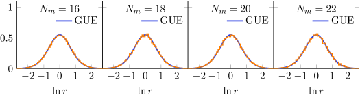
Figure 1: Statistical distribution of the ratio $r$ of two consecutive level spacings for the ${\cal N}=0$ SYK model with $q=6$. The number of realizations used for averaging was $10^{3}$ for $N_{m}=16$, $10^{2}$ for $N_{m}=18$ and $20$, and 10 for $N_{m}=22$. The blue lines are surmises for the RMT classes in table 3.

Universality at the hard edge

In class C and D the origin is a special point due to the spectral mirror symmetry, and the level statistics near zero shows universal fluctuations different from those in the bulk of the spectrum Altland:1997zz . Their form is solely determined by the global symmetries of the Hamiltonian and is insensitive to microscopic details of interactions. In figure 2 we compare the distributions of the near-zero energy levels of the ${\cal N}=0$ SYK model with $q=6$ and those of RMT, finding nearly perfect agreement. The nonzero (zero) intercept at $\lambda=0$ in class D (class C) directly reflects the fact that $\alpha=0$ for class D ($\alpha=2$ for class C), where $\alpha$ is the index listed in table 1.

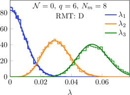
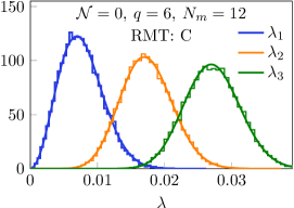
Figure 2: Distributions of the eigenvalues of $H$ with smallest absolute values in the ${\cal N}=0$ SYK model with $q=6$ and $J=1$, compared with the predictions (solid lines) of the RMT classes in table 3. The number of independent random samples is $10^{4}$ for each plot. The small deviations from RMT for the third nonzero eigenvalue are interpreted to be effects of finite $N_{m}$.

3.4 Overview of the ${\cal N}=0$ SYK model with complex fermions

We finally comment on the non-supersymmetric SYK model with complex fermions Sachdev:2015efa ; You:2016ldz ; Fu:2016yrv ; Davison:2016ngz ; Bulycheva2017 . The Hamiltonian reads $H=\sum_{i,j,k,\ell=1}^{N_{c}}J_{ij;k\ell}\overline{c}_{i}\overline{c}_{j}c_{k}c_{\ell}-\mu F$, where $\mu$ is the chemical potential for the fermion number operator $F$ in (2) and the coupling is a complex Gaussian random variable obeying $J_{ij;k\ell}=-J_{ji;k\ell}=-J_{ij;\ell k}=J_{k\ell;ij}^{*}$. Since $H$ preserves the fermion number, $H$ as a matrix has a block-diagonal structure representing each eigenspace of $F=0,1,\dots,N_{c}$ . There is no antiunitary symmetry for $H$ and consequently the levels collected in each block of $H$ would obey GUE. Intriguingly, one can amend $H$ by adding correction terms so that it commutes with $P$ You:2016ldz ; Fu:2016yrv . In this case, the half-filled sector $F=N_{c}/2$ (which only exists for $N_{c}$ even) is symmetric under $P$ and its level statistics becomes either GOE (if $P^{2}=+1$) or GSE (if $P^{2}=-1$). In all other sectors, the level statistics remains GUE, but there arises a degeneracy between the sector $F=k$ and the sector $F=N_{c}-k$ for $k\neq N_{c}/2$ since they are mapped to each other by $P$.

4 ${\cal N}=1$ SYK model

4.1 Classification

The supersymmetric generalization of the SYK model was introduced in Fu:2016vas (see also Anninos:2016szt ; Gross:2016kjj ; Sannomiya:2016mnj ; Yoon:2017gut ; Peng:2017spg ). The model with ${\cal N}=1$ SUSY has the Hamiltonian $H=Q^{2}$ with supercharge

$$Q=i^{({\hat{q}}-1)/2}\!\!\!\sum_{1\leq i_{1}<\cdots<i_{{\hat{q}}}\leq N_{m}}C_{i_{1}i_{2}\cdots i_{{\hat{q}}}}\chi_{i_{1}}\chi_{i_{2}}\cdots\chi_{i_{\hat{q}}}\,,$$ (9)

where $1\leq{\hat{q}}\leq N_{m}$ is an odd integer. (Note that $Q^{\dagger}=Q$.) In this case $H$ involves terms with up to $2{\hat{q}}-2$ fermions. The couplings $C_{i_{1}i_{2}\cdots i_{{\hat{q}}}}$ are independent real Gaussian variables with mean $\langle C_{i_{1}i_{2}\cdots i_{{\hat{q}}}}\rangle=0$ and variance $\langle C^{2}_{i_{1}i_{2}\cdots i_{{\hat{q}}}}\rangle=\frac{({\hat{q}}-1)!}{N_{m}^{{\hat{q}}-1}}J$ for some $J>0$ . The ground-state energy of this model is evidently nonnegative. In Fu:2016vas a strictly positive ground-state energy that decreases exponentially with $N$ was obtained numerically, indicating that SUSY is dynamically broken at finite $N$ and restored only in the large-$N$ limit.

It is easy to verify the simple relation

$$\rho_{H}(\lambda)=\frac{1}{\sqrt{\lambda}}\rho_{Q}(\sqrt{\lambda}\,)\quad\qquad(\lambda\geq 0)$$ (10)

between the spectral densities of $H$ and $Q$, where $\rho_{H}(\lambda)\equiv\big{\langle}\!\operatorname{Tr}\delta(\lambda-H)\big{\rangle}$ and $\rho_{Q}(X)\equiv\big{\langle}\!\operatorname{Tr}\delta(X-Q)\big{\rangle}$ . Equation (10) reveals that the level density of $H$ would blow up as $\lambda^{-1/2}$ near zero if $Q$ had a nonzero density of states at the origin for large $N_{m}$. This blow-up was indeed seen in the exact diagonalization analysis Li:2017hdt as well as in analytical studies of the low-energy Schwarzian theory Fu:2016vas ; Stanford:2017thb ; Mertens:2017mtv . Since $Q$ is more fundamental than $H$ we will focus on the level structure of $Q$ below, viewing it as a matrix acting on the many-body Fock space.

The random matrix classification for ${\hat{q}}=3$ has recently been put forward in Li:2017hdt . Here we will generalize this to all odd ${\hat{q}}$, with emphasis on the difference of symmetry classes between ${\hat{q}}=1$ (mod 4) and ${\hat{q}}=3$ (mod 4). The main theoretical novelty in the ${\cal N}=1$ SYK model is the fact that $Q$ anticommutes with the fermion parity operator $(-1)^{F}$. Thus $(-1)^{F}$ plays the role of $\gamma_{5}$ for the Dirac operator in QCD and naturally induces a block structure $\displaystyle\begin{pmatrix}0&\framebox{$*$}\\ \framebox{$*$}^{\dagger}&0\end{pmatrix}$ for $Q$. The spectrum of $Q$ is therefore symmetric under $\lambda\leftrightarrow-\lambda$. Since the block $\framebox{$*$}$ is a square matrix, there are no topological zero modes, i.e., all eigenvalues of $Q$ are nonzero unless fine-tuning of the matrix elements is performed. From the relation $H=Q^{2}$ we conclude that all eigenvalues of $H$ should be at least twofold degenerate.

Following Li:2017hdt we introduce a new antiunitary operator $R\equiv P(-1)^{F}$. We have

$$PQP=(-1)^{({\hat{q}}-1)/2}\eta Q\qquad\text{and}\qquad RQR=(-1)^{({\hat{q}}-1)/2+N_{c}+1}\eta Q\,,$$ (11)

where $N_{c}=N_{m}/2$ as before and $\eta$ is given in (6). These relations, combined with table 1, lead to the classification of $Q$ shown in table 4 for ${\hat{q}}=1$ (mod 4) and table 5 for ${\hat{q}}=3$ (mod 4). By comparing the (anti-)commutators in each table, we see that the roles of $P$ and $R$ are exchanged for ${\hat{q}}=1$ and 3. Consequently the positions of BdG(CI) and BdG(DIII-even) are exchanged. In these tables we made it clear that we are considering chGOE and chGSE in the topologically trivial sector $\nu=0$.

Table 4: Symmetry classification of $Q$ in the ${\cal N}=1$ SYK model for ${\hat{q}}=1$ (mod 4). For the block structure of each class we refer to table 1.

​​​​ $\begin{array}[]{c}\text{\footnotesize${\cal N}=1$ SYK}\vspace{-4pt}\\ {\footnotesize{\hat{q}}=1~{}\text{(mod~{}4)}}\end{array}$ ​​​​	$P^{2}$	$R^{2}$	$\begin{array}[]{c}\text{\footnotesize(anti-)}\vspace{-8pt}\\ \text{\footnotesize\!\!\!\! commutators \!\!\!\!}\end{array}$	$\beta$	class of $Q$	$\begin{array}[]{c}\text{\footnotesize degeneracy}\vspace{-7pt}\\ \text{\footnotesize\!\!\!\!of levels in $H$\!\!\!\!}\end{array}$
​$N_{m}=0$ (mod 8)​	$+1$	$+1$	$\begin{array}[]{c}\{P,Q\}=0\\ {[R,Q]=0}\end{array}$	1	​​​​​​​ $\begin{array}[]{c}\text{chGOE (BDI)}\vspace{-2pt}\\ \nu=0\end{array}$ ​​​​​​​	2
​$N_{m}=2$ (mod 8)​	$+1$	$-1$	$\begin{array}[]{c}{[P,Q]=0}\\ \{R,Q\}=0\end{array}$	1	BdG (CI)	2
​$N_{m}=4$ (mod 8)​	$-1$	$-1$	$\begin{array}[]{c}\{P,Q\}=0\\ {[R,Q]=0}\end{array}$	4	$\begin{array}[]{c}\text{chGSE (CII)}\vspace{-2pt}\\ \nu=0\end{array}$	4
​$N_{m}=6$ (mod 8)​	$-1$	$+1$	$\begin{array}[]{c}{[P,Q]=0}\\ \{R,Q\}=0\end{array}$	4	$\begin{array}[]{c}\text{BdG}\vspace{-4pt}\\ \text{(DIII-even)}\end{array}$	4

Table 5: Symmetry classification of $Q$ in the ${\cal N}=1$ SYK model for ${\hat{q}}=3$ (mod 4). This table is consistent with Li:2017hdt . For the block structure of each class we refer to table 1.

​​​​ $\begin{array}[]{c}\text{\footnotesize${\cal N}=1$ SYK}\vspace{-4pt}\\ {\footnotesize{\hat{q}}=3~{}\text{(mod~{}4)}}\end{array}$ ​​​​	$P^{2}$	$R^{2}$	$\begin{array}[]{c}\text{\footnotesize(anti-)}\vspace{-8pt}\\ \text{\footnotesize\!\!\!\! commutators \!\!\!\!}\end{array}$	$\beta$	class of $Q$	$\begin{array}[]{c}\text{\footnotesize degeneracy}\vspace{-7pt}\\ \text{\footnotesize\!\!\!\!of levels in $H$\!\!\!\!}\end{array}$
​$N_{m}=0$ (mod 8)​	$+1$	$+1$	$\begin{array}[]{c}[P,Q]=0\\ \{R,Q\}=0\end{array}$	1	$\begin{array}[]{c}\!\!\!\text{chGOE (BDI)}\!\!\!\vspace{-2pt}\\ \nu=0\end{array}$	2
​$N_{m}=2$ (mod 8)​	$+1$	$-1$	$\begin{array}[]{c}\{P,Q\}=0\\ {[R,Q]=0}\end{array}$	4	$\begin{array}[]{c}\text{BdG}\vspace{-4pt}\\ \text{(DIII-even)}\end{array}$	4
​$N_{m}=4$ (mod 8)​	$-1$	$-1$	$\begin{array}[]{c}[P,Q]=0\\ \{R,Q\}=0\end{array}$	4	$\begin{array}[]{c}\text{chGSE (CII)}\vspace{-2pt}\\ \nu=0\end{array}$	4
​$N_{m}=6$ (mod 8)​	$-1$	$+1$	$\begin{array}[]{c}\{P,Q\}=0\\ {[R,Q]=0}\end{array}$	1	BdG (CI)	2

One can also consider a superposition of multiple fermionic operators in the supercharge, e.g, $Q=i\sum_{ijk}C_{ijk}\chi_{i}\chi_{j}\chi_{k}+\sum_{i}D_{i}\chi_{i}$, where $\{C_{ijk}\}$ and $\{D_{i}\}$ are independent real Gaussian couplings. Then $Q$ fails to commute or anti-commute with $P$ and $R$ and the symmetry class is changed: $Q$ now belongs to the $\beta=2$ chGUE (AIII) class with $\nu=0$. There is no degeneracy of eigenvalues for $Q$ while all eigenvalues of $H=Q^{2}$ are two-fold degenerate since $\{(-1)^{F},Q\}=0$.

In all cases considered above for ${\cal N}=1$, the symmetry classes differ from the Wigner-Dyson classes because of the presence of chiral symmetry $(-1)^{F}$. This difference manifests itself in distinctive level correlations near the origin (universality at the hard edge). In order to expose this in the thermal ${\cal N}=1$ SYK model, the temperature must be lowered to the scale of the smallest eigenvalue of $H$. This is exponentially small in $N_{m}$.

4.2 Numerical simulations

Level correlations in the bulk

Previously, the level statistics in the bulk of the energy spectrum for the ${\cal N}=1$ SYK model with ${\hat{q}}=3$ was studied in Li:2017hdt and results consistent with table 5 were reported. Here we report the first numerical analysis of the bulk statistics for the ${\cal N}=1$ SYK model with ${\hat{q}}=5$ via exact diagonalization, to test table 4. To identify the symmetry class, we again used the ratio of two consecutive level spacings. Our numerical results are displayed in figure 3. Excellent agreement with the RMT curves of the symmetry classes predicted by table 4 is observed. This evidences the existence of quantum chaotic dynamics in this model and corroborates our classification scheme.

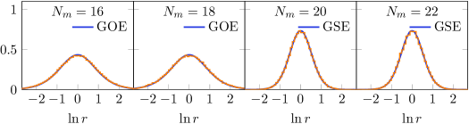
Figure 3: Distribution of the ratio $r$ of two consecutive level spacings in the ${\cal N}=1$ SYK model with ${\hat{q}}=5$. The number of realizations used for averaging was $10^{3}$ for $N_{m}=16$, $100$ for $N_{m}=18$ and $22$, and $200$ for $N_{m}=20$. The blue lines are surmises for the RMT classes in table 4.

Universality at the hard edge

Next we proceed to the investigation of universality of the level distributions near the origin. In contrast to the ${\cal N}=0$ SYK model, whose hard edge at $\lambda=0$ was in the middle of the spectrum, the fluctuations of the smallest eigenvalues of $Q$ (or $H$) are of direct physical significance for the low-temperature thermodynamics of the ${\cal N}=1$ SYK model. We have

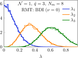
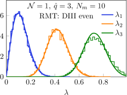
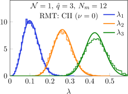
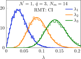
Figure 4: Distributions of the smallest 3 eigenvalues of $Q$ in (9) in the ${\cal N}=1$ SYK model with ${\hat{q}}=3$ and $J=1$, compared with the predictions (solid lines) of the RMT classes in table 5. The number of independent random samples is $10^{4}$ for each plot. As in figure 2, the small deviations from RMT for $\lambda_{3}$ are interpreted to be effects of finite $N_{m}$.

Figure 5: Same as figure 4 but for ${\hat{q}}=5$ and compared with the RMT predictions in table 4.

numerically studied the distributions of the smallest three eigenvalues of $Q$ for the ${\cal N}=1$ SYK model with ${\hat{q}}=3$ and $5$ for varying $N_{m}$. (The twofold degeneracy of each level was resolved in the case of $\beta=4$.) The results for ${\hat{q}}=3$ and $5$ are shown in figures 4 and 5, respectively. They show very good agreement with the corresponding RMT predictions in tables 5 and 4. The smallest eigenvalue approaches zero from above for larger $N_{m}$, indicating restoration of SUSY in the large-$N_{m}$ limit as already reported in Fu:2016vas .

We note that the RMT classes chGOE (BDI) and chGSE (CII) were originally invented and exploited in attempts to theoretically understand fluctuations of small eigenvalues of the Euclidean QCD Dirac operator with special antiunitary symmetries in a finite volume Verbaarschot:1994qf ; Verbaarschot:1994ia ; Halasz:1995qb ; Verbaarschot:1997bf ; Nagao:2000cb , related to spontaneous breaking of chiral symmetry through the Banks-Casher relation Banks:1979yr . The RMT predictions agree well with the Dirac spectra taken from lattice QCD simulations BerbenniBitsch:1997tx . It is a nontrivial observation that the smallest energy levels of the ${\cal N}=1$ SYK model, which set the scale for the spontaneous breaking of SUSY, obey the same statistics as the eigenvalues of the Dirac operator in QCD, which has totally different microscopic interactions compared to the SYK model. This is yet another example for random matrix universality.

5 Interlude: a simple model bridging the gap between ${\cal N}=1$ and $2$

5.1 Motivation and definition

The SYK model with ${\cal N}=2$ SUSY Fu:2016vas has the Hamiltonian $H=\{Q,\overline{Q}\}$ with two supercharges $Q$ and $\overline{Q}$, each comprising an odd number of complex fermions. This model preserves the $\text{U}(1)$ fermion number exactly, so that the Hamiltonian is block-diagonal in the fermion-number eigenbasis. As shown by the Witten-index computation in Fu:2016vas , the Hamiltonian has an extensive number of exact zero modes and SUSY is unbroken at finite $N_{c}$ . These features are in marked contrast to the ${\cal N}=1$ SYK model, where the fermion number is only conserved modulo 2, the Hamiltonian is positive definite with no exact zero modes, and SUSY is spontaneously broken at finite $N_{c}$ .

While there is no logical obstacle to moving from ${\cal N}=1$ to $2$, it is helpful to have a simple model that serves as a bridge between these two theories. The model we designed for this purpose is defined by the Hamiltonian $H=M^{2}$ with the Hermitian operator

$$M\equiv i^{p/2}\!\!\!\!\!\sum_{1\leq j_{1}<\cdots<j_{p}\leq N_{c}}\!\!\!\!\big{(}Z_{j_{1}\cdots j_{p}}\,c_{j_{1}}\cdots c_{j_{p}}+\overline{Z_{j_{1}\cdots j_{p}}}\,\overline{c}_{j_{1}}\cdots\overline{c}_{j_{p}}\big{)}\,,$$ (12)

where $1\leq p\leq N_{c}$ is an even integer and $Z_{j_{1}\cdots j_{p}}$ are independent complex Gaussian random variables with mean zero and $\langle\overline{Z_{ab}}Z_{ab}\rangle=2J/N_{c}^{2}$ for some $J>0$. The creation and annihilation operators $\overline{c}_{a}$ and $c_{a}$ were introduced in section 3.1. Because of $M=M^{\dagger}$ we have $H\geq 0$, similarly to the supersymmetric SYK models. If we forcefully substitute $p=3$ and let $i^{p/2}\to i$, then $M=Q+\overline{Q}$ and $H=M^{2}=\{Q,\overline{Q}\}$, i.e., the ${\cal N}=2$ SYK model is recovered (see section 6). What difference emerges if we retain an even number of fermions in $M$? Of course it makes $M$ a bosonic operator and destroys SUSY. At this cost, however, we gain three new features that were missing in the ${\cal N}=1$ SYK model: (i) the fermion number is conserved modulo $2p$ (rather than modulo $2$), (ii) $H$ has a large number of exact zero modes, and (iii) an interplay between $N_{c}$ and $F$ emerges in the symmetry classification of energy-level statistics. The last point is especially intriguing since this property is shared by the ${\cal N}=2$ SYK model (section 6). This is why we regard this model as “intermediate” between the ${\cal N}=1$ and ${\cal N}=2$ SYK models. Studying the level structure of this exotic model provides a useful digression before tackling the ${\cal N}=2$ case.

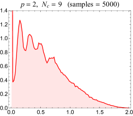
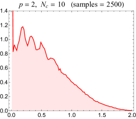
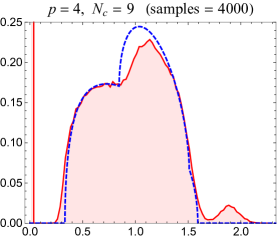
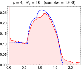
Figure 6: Spectral density of $M$ in (12) for $p=2$ (top) and $4$ (bottom) at $N_{c}=9$ and $10$, averaged over many random samples. Since the spectra are symmetric about $0$, only the nonnegative part is shown. The sharp peak at the origin in each plot represents the density of exact zero modes. In all plots $J=1$ and the total density is normalized to 1. The blue dashed lines in the bottom plots are analytic approximations (20) based on the Marčenko-Pastur law.

By exact diagonalization we have numerically computed the spectral density of $M$ for $p=2$ and $4$, see figure 6. In all plots there is a delta function at zero due to the macroscopic number of zero-energy states. Interestingly, the global shape never resembles Wigner’s semicircle but rather depends sensitively on both $p$ and $N_{c}$. For $p=2$ we observe oscillations in the middle of the spectrum, for which we currently do not have a simple explanation. The case $p=2$ could be more the exception than the rule, much like the $q=2$ SYK model that is solvable and nonchaotic Maldacena:2016hyu ; Gross:2016kjj ; Cotler:2016fpe unlike its $q>2$ counterparts.

For both $p=2$ and $4$, a close inspection of the plots near the origin reveals that for odd $N_{c}$ there is a dip of the density around the origin, indicating that small nonzero levels are repelled from the origin, while there is no such repulsion for even $N_{c}$ . The same tendency of the spectral density (albeit with the parity of $N_{c}$ reversed) has been observed for the ${\cal N}=2$ SYK model, too Stanford:2017thb . We will give a simple explanation of this phenomenon later.

5.2 Classification for $p=2$

To make the presentation as simple as possible, we shall begin with $p=2$, in which case the fermion number $F$ is conserved modulo $4$. The Hilbert space $V$ of $N_{c}$ complex fermions can be arranged into a direct sum of four spaces $\overline{V}_{0,1,2,3}$, where $\overline{V}_{f}$ is the eigenspace of $F$ corresponding to $F=f$ (mod 4), i.e.,

$$V=\overline{V}_{0}\oplus\overline{V}_{1}\oplus\overline{V}_{2}\oplus\overline{V}_{3}$$ (13)

with $\dim(V)=\sum_{f=0}^{3}\dim(\overline{V}_{f})=2^{N_{c}}$ and

$$\overline{D}_{f}\equiv\mathrm{dim}(\overline{V}_{f})=\!\!\!\sum_{k=0}^{\lfloor(N_{c}-f)/4\rfloor}\binom{N_{c}}{4k+f}\,.$$ (14)

The numbers $\overline{D}_{0,1,2,3}$ are listed for $3\leq N_{c}\leq 10$ in table 6. Since there is no nonzero matrix element of $M$ between states with different parity of $F$ we have $M=\scalebox{0.8}{$\displaystyle\begin{pmatrix}0&A_{0}\\ A_{0}^{\dagger}&0\end{pmatrix}\oplus\begin{pmatrix}0&A_{1}\\ A_{1}^{\dagger}&0\end{pmatrix}$}$, where the first (second) term corresponds to $\overline{V}_{0}\oplus\overline{V}_{2}$ ($\overline{V}_{1}\oplus\overline{V}_{3}$). The chiral structure in each term is due to the chiral symmetry $\{i^{F},M\}=0$, which ensures the spectral mirror symmetry of $M$.

It should be stressed that $A_{0}$ and $A_{1}$ are in general rectangular. When they become a square matrix can be read off from table 6. These cases are colored in red and green. They only occur for even $N_{c}$ (which is also true for $p=4$, see table 7 below). On the other hand, for odd $N_{c}$ , both $A_{0}$ and $A_{1}$ are rectangular. As is well known from studies in chiral RMT Verbaarschot:1997bf ; Verbaarschot:2000dy , in that case the nonzero eigenvalues of $M$ (i.e., the nonzero singular values of $A_{0}$ and $A_{1}$) are pushed away from the origin by the large number of exact zero modes. Indeed, $\alpha$ in table 1 is proportional to the number of zero modes, and large $\alpha$ suppresses the joint probability density of eigenvalues near zero. This leads to the dip around the origin in the left plots of figure 6. However, for even $N_{c}$ , in the subspaces without exact zero modes there is no repulsion of the nonzero modes from the origin, and thus no dip of the density (which is summed over all subspaces) shows up near zero.

In order to understand the level degeneracy in each sector correctly, we must figure out the antiunitary symmetries of the matrix $M$. We use the particle-hole operator $P$ in (4) again. In addition, we define another antiunitary operator $S\equiv P\cdot i^{F}$. One can show

$$\{P,M\}=0\qquad\text{and}\qquad[S,M]=0\qquad\text{for all $N_{c}$\,.}$$ (15)

Both $P^{2}$ and $S^{2}$ are tabulated in table 6, but extra care is needed for $S$ because $S^{2}$ is not just $\pm 1$ but a nontrivial operator that depends on $F$.

Table 6: Model (12) for $p=2$. We list the dimensions (14) of the eigenspaces of $F$ (mod 4). Uncolored blocks belong to chGUE (AIII)_β=2, while    : chGSE (CII)_β=4 with $\nu=|\overline{D}_{1}-\overline{D}_{3}|/2$,    : BdG (DIII-even)_β=4,    : chGOE (BDI)_β=1 with $\nu=|\overline{D}_{0}-\overline{D}_{2}|$, and    : BdG (CI)_β=1. Details of each class can be found in table 1. Also shown are the squares of the antiunitary operators $P$ and $S$. The symmetry pattern is periodic in $N_{c}$ with period $4$.

$N_{c}$	3	4	5	6	7	8	9	10
$\overline{D}_{0}$	1	2	6	16	36	72	136	256
$\overline{D}_{2}$	3	6	10	16	28	56	120	256
​​​$\#$Zero modes​​​	2	4	4	0	8	16	16	0
$\overline{D}_{1}$	3	4	6	12	28	64	136	272
$\overline{D}_{3}$	1	4	10	20	36	64	120	240
​​​$\#$Zero modes​​​	2	0	4	8	8	0	16	32
$P^{2}$	$-1$	1	1	$-1$	$-1$	1	1	$-1$
$S^{2}$	$(-1)^{F+1}i$	$(-1)^{F}$	$(-1)^{F+1}i$	$(-1)^{F}$	$(-1)^{F+1}i$	$(-1)^{F}$	$(-1)^{F+1}i$	$(-1)^{F}$

For even $N_{c}$ , each chiral block belongs to one of chGSE (CII)_β=4, BdG (DIII-even)_β=4, chGOE (BDI)_β=1, and BdG (CI)_β=1 according to the values of $P^{2}$ and $S^{2}$ (cf. table 1). In the $\beta=4$ classes, every nonzero level must come in quadruplets $(\lambda,\lambda,-\lambda,-\lambda)$ due to Kramers degeneracy and chiral symmetry.

For odd $N_{c}$ , $P$ maps a state in $\overline{V}_{0}\oplus\overline{V}_{2}$ to $\overline{V}_{1}\oplus\overline{V}_{3}$ and vice versa. Therefore the nonzero levels of $M$ in $\overline{V}_{0}\oplus\overline{V}_{2}$ must be degenerate with those in $\overline{V}_{1}\oplus\overline{V}_{3}$. Since there is no antiunitary symmetry acting within each chiral block, all uncolored sectors in table 6 belong to chGUE (AIII).

This completes the algebraic classification of the model (12) for $p=2$ based on RMT. This classification is periodic in $N_{c}$ with period $4$ as can be seen from table 6. We have numerically checked the level degeneracy of $M$ in each sector for various $N_{c}$ and confirmed consistency with our classification. In this process we found, surprisingly, that levels often show a large (e.g., 16-fold) degeneracy that cannot be accounted for by our antiunitary symmetries $P$ and $S$. Such a large degeneracy, which presumably is responsible for the wavy shape in the upper plots of figure 6 and makes the level spacing distribution for $p=2$ deviate from RMT, was not observed for $p=4$. We interpret this as an indication that the model with $p=2$ is just too simple to show quantum chaos and therefore do not investigate it further.

5.3 Classification for $p=4$

As a more nontrivial case we now study the $p=4$ model, which preserves $F$ (mod 8). This time the Hilbert space decomposes as $V=\bigoplus\limits_{f=0}^{7}\overline{V}_{f}$ with

$$\overline{D}_{f}\equiv\dim(\overline{V}_{f})=\sum_{k=0}^{\lfloor(N_{c}-f)/8\rfloor}\!\!\binom{N_{c}}{8k+f}\,.$$ (16)

$M$ acquires a block-diagonal form, $M=\scalebox{0.8}{$\displaystyle\begin{pmatrix}0&A_{0}\\ A_{0}^{\dagger}&0\end{pmatrix}\oplus\begin{pmatrix}0&A_{1}\\ A_{1}^{\dagger}&0\end{pmatrix}\oplus\begin{pmatrix}0&A_{2}\\ A_{2}^{\dagger}&0\end{pmatrix}\oplus\begin{pmatrix}0&A_{3}\\ A_{3}^{\dagger}&0\end{pmatrix}$}$, where the terms correspond to $\overline{V}_{0}\oplus\overline{V}_{4}$, $\overline{V}_{1}\oplus\overline{V}_{5}$, $\overline{V}_{2}\oplus\overline{V}_{6}$, and $\overline{V}_{3}\oplus\overline{V}_{7}$, respectively. As a consequence, the spectrum of $M$ enjoys a mirror symmetry as in the model with $p=2$. Let us define an antiunitary operator $\widetilde{S}\equiv P\cdot\kappa^{F}$, where $\kappa\equiv e^{i\pi/4}$ is the 8-th root of unity and $P$ was defined in (4). One can show

$$[P,M]=0\qquad\text{and}\qquad\{\widetilde{S},M\}=0\qquad\text{for all $N_{c}$\,.}$$ (17)

Table 7: Model (12) for $p=4$. We list the dimensions (16) of the eigenspaces of $F$ (mod 8). Uncolored blocks belong to chGUE (AIII)_β=2, while    : chGSE (CII)_β=4 with $\nu=|\overline{D}_{i}-\overline{D}_{i+4}|/2$,    : BdG (DIII-even)_β=4,    : chGOE (BDI)_β=1 with $\nu=|\overline{D}_{i}-\overline{D}_{i+4}|$, and    : BdG (CI)_β=1. Details of each class can be found in table 1. The mark $({\color[rgb]{1,0,0}2})$ after the number of positive levels of $M$ indicates that those levels are twofold degenerate, e.g., $20\,({\color[rgb]{1,0,0}2})$ means $10$ pairs. In each block of given $N_{c}$ there is an equal number of positive and negative levels because of chiral symmetry, $\{\kappa^{F},M\}=0$. Also shown are the squares of the antiunitary operators $P$ and $\widetilde{S}$. The symmetry pattern is periodic in $N_{c}$ with period $8$.

$N_{c}$	7	8	9	10	11	12	13	14
$\overline{D}_{0}$	1	2	10	46	166	496	1288	3004
$\overline{D}_{4}$	35	70	126	210	330	496	728	1092
​​ $\begin{array}[]{c}\text{$\#$\,Positive}\vspace{-4pt}\\ \text{levels of $M$}\end{array}$ ​​​	1	2	10	46	166	496	728	1092
$\overline{D}_{1}$	7	8	10	20	66	232	728	2016
$\overline{D}_{5}$	21	56	126	252	462	792	1288	2016
​​ $\begin{array}[]{c}\text{$\#$\,Positive}\vspace{-4pt}\\ \text{levels of $M$}\end{array}$ ​​​	7	8	10	​​​ 20 (2)​​​	66	232	728	​​2016 (2)​​​
$\overline{D}_{2}$	21	​ 28 ​	36	46	66	132	364	1092
$\overline{D}_{6}$	7	28	84	210	462	924	1716	3004
​​ $\begin{array}[]{c}\text{$\#$\,Positive}\vspace{-4pt}\\ \text{levels of $M$}\end{array}$ ​​​	7	28	36	46	66	132	364	1092
$\overline{D}_{3}$	35	56	84	120	166	232	364	728
$\overline{D}_{7}$	1	8	36	120	330	792	1716	3432
​​ $\begin{array}[]{c}\text{$\#$\,Positive}\vspace{-4pt}\\ \text{levels of $M$}\end{array}$ ​​​	1	8	36	​​​120 (2)​​​	166	232	364	​​728 (2)​​
$P^{2}$	$-1$	1	1	$-1$	$-1$	1	1	$-1$
$\widetilde{S}^{2}$	​​$-\kappa^{2F+1}$​​	​$\kappa^{2F}$​	$\kappa^{2F-1}$	​​​​ $\kappa^{2F+2}$ ​​​​	$\kappa^{2F+1}$	​​$-\kappa^{2F}$​​	$\kappa^{2F+3}$	$\kappa^{2F-2}$

The dimension of each subspace of $V$ is listed for $7\leq N_{c}\leq 14$ in table 7. As for $p=2$, the particle-hole operator $P$ generates degeneracies between distinct chiral blocks. For instance, at $N_{c}=11$, the 166 distinct positive levels in $\overline{V}_{0}\oplus\overline{V}_{4}$ are degenerate with those in $\overline{V}_{3}\oplus\overline{V}_{7}$. The symmetry classification is just a rerun of our arguments for $p=2$ and therefore omitted here. We have numerically confirmed that table 7 gives the correct degeneracy of levels. (Unlike for $p=2$, we did not observe any unexpected further degeneracies.)

5.4 Global spectral density

Table 7 not only provides a symmetry classification but also enables us to derive a fairly simple analytic approximation to the global spectral density. Let us recall the so-called Marčenko-Pastur law MP1967 : suppose $X$ is a complex $L\times N$ matrix with $L\leq N$ whose elements are independently and identically distributed with $\langle X_{ij}\rangle=0$ and $\langle|X_{ij}|^{2}\rangle=\sigma^{2}<\infty$. Let us denote the $L$ eigenvalues of $\sqrt{XX^{\dagger}}$ by $\{\xi_{i}\}\geq 0$. Then for $L,N\to\infty$ with $L/N\in(0,1]$ fixed, the probability distribution of $\{\xi_{i}\}$ takes on the limit

$$P_{L,N}(\sigma;\xi)=\frac{1}{\sqrt{N}\sigma}F\left(\frac{L}{N},\frac{\xi}{\sqrt{N}\sigma}\right),$$ (18)

where

$$F(\alpha,x)\equiv\begin{cases}\displaystyle\frac{1}{\pi\alpha x}\sqrt{\left[(1+\sqrt{\alpha})^{2}-x^{2}\right]\left[x^{2}-(1-\sqrt{\alpha})^{2}\right]}&\text{for }x\in[1-\sqrt{\alpha},1+\sqrt{\alpha}\,]\,,\\ ~{}~{}0&\text{otherwise}\,.\end{cases}$$ (19)

This function satisfies the normalization $\int_{0}^{\infty}dx\,F(\alpha,x)=1$ for all $\alpha\in(0,1]$. We now exploit this law to describe the global density of our $p=4$ model, shown previously in figure 6. Whether (18) works quantitatively or not is not obvious a priori because the matrix elements of (12) are far from statistically independent, but rather strongly correlated. Putting this worry aside, let us consider the $N_{c}=9$ case first. According to table 7, there are four chiral blocks, and two of them are copies of the other two, so we should sum just two Marčenko-Pastur distributions. For $N_{c}=10$, we have to sum three. Taking into account that the global density in figure 6 counts both positive modes and exact zero modes, we obtain formulas with the correct normalization,

$$P^{(p=4,N_{c}=9)}(\sigma;\xi) =\frac{2\big{[}10\cdot P_{10,126}(\sigma;\xi)+36\cdot P_{36,84}(\sigma;\xi)\big{]}}{2^{9}-2(10+36)}\,,$$ (20a)

$$P^{(p=4,N_{c}=10)}(\sigma;\xi) =\frac{2\cdot 46\cdot P_{46,210}(\sigma;\xi)+20\cdot P_{20,252}(\sigma;\xi)+120\cdot P_{120,120}(\sigma;\xi)}{2^{10}-(2\cdot 46+20+120)}\,.$$ (20b)

The parameter $\sigma$ has to be tuned to achieve the best fit to the data because RMT does not know the typical energy scale of the model. The results of the fits displayed in the bottom plots of figure 6 show impressive quantitative agreement. We also notice a shortage of levels near the peak density, as well as a leakage of levels toward larger values. Even though the agreement is not perfect it is intriguing that a naïve ansatz such as (20) is sufficient to account for the shape of the global density. We tried a similar fit for $p=2$ as well but did not find any agreement even at a qualitative level, probably due to the nonchaotic character of the $p=2$ model as described before.

5.5 Numerical simulations

Level correlations in the bulk

We numerically checked the bulk statistics (GOE/GUE/GSE). As there are quite a few chiral blocks in table 7 we did not check all of them but concentrated on three cases: (i) the $\overline{V}_{3}\oplus\overline{V}_{7}$ sector for $N_{c}=10$, (ii) the $\overline{V}_{3}\oplus\overline{V}_{7}$ sector for $N_{c}=11$, and (iii) the $\overline{V}_{0}\oplus\overline{V}_{4}$ sector for $N_{c}=12$. To identify the symmetry classes we again used the probability distribution of the ratio of two consecutive level spacings. Our numerical results are displayed in figure 7, where excellent agreement with the respective symmetry classes predicted by table 7 is found. This corroborates our symmetry classification scheme.

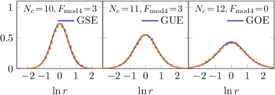
Figure 7: Distribution of the ratio $r$ of two consecutive level spacings of $M$ in (12) with $p=4$. The number of random samples used for averaging was 180 for $N_{c}=10$, 120 for $N_{c}=11$, and 40 for $N_{c}=12$. The blue lines are surmises for the RMT classes in table 7.

Universality at the hard edge

To check the universality of the level distributions near the origin, we have numerically generated $M$ randomly and computed the smallest 3 eigenvalues. (In the sector of $F=3$ (mod 4) for $N_{c}=10$, each twofold degenerate pair of levels was counted only once.) The results shown in figure 8 display excellent agreement with RMT as predicted by table 7.

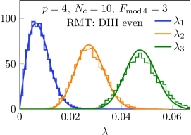
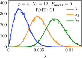
Figure 8: Distributions of the smallest three eigenvalues of $M$ in (12) with $p=4$ and $J=1$ for two sets of $N_{c}$ and $F$ (mod 4). Comparison is made with the predictions (solid lines) of the RMT classes in table 7. The number of independent random samples is $10^{4}$ for each plot. The small deviations from RMT are again effects of finite $N_{c}$.

6 ${\cal N}=2$ SYK model

6.1 Preliminaries

The ${\cal N}=2$ SYK model Fu:2016vas ; Yoon:2017gut ; Peng:2017spg has significantly different properties from its ${\cal N}=1$ cousin. The Hamiltonian is defined by $H=\{Q,\overline{Q}\}$ with two supercharges

$$Q=i\!\!\!\!\sum_{1\leq i<j<k\leq N_{c}}\!\!\!\!X_{ijk}c_{i}c_{j}c_{k}\qquad\text{and}\qquad\overline{Q}=i\!\!\!\!\sum_{1\leq i<j<k\leq N_{c}}\!\!\!\!\overline{X_{ijk}}\;\overline{c}_{i}\overline{c}_{j}\overline{c}_{k}$$ (21)

that are nilpotent, $Q^{2}=\overline{Q}^{2}=0$, where the couplings $X_{ijk}$ are independent complex Gaussian random variables obeying $\langle X_{ijk}\overline{X_{ijk}}\rangle=2J/N_{c}^{2}$ . Apart from the random disorder, this model is somewhat similar to lattice models with exact SUSY Nicolai:1976xp ; Nicolai:1977qx ; Fendley:2002sg ; Fendley:2003je ; Fendley:2005ae ; Eerten2005 . The model can be generalized so that $Q$ and $\overline{Q}$ involve ${\hat{q}}$ fermions with ${\hat{q}}$ odd Fu:2016vas . We postpone this generic case to section 6.5 and for the moment focus on ${\hat{q}}=3$, i.e., (21). As for the operator $P$ in (4), we have

(29)

As shown in Fu:2016vas ; Stanford:2017thb ; Mertens:2017mtv , $H$ possesses a number of exactly zero eigenvalues, so SUSY is not spontaneously broken in contrast to the ${\cal N}=1$ model. Moreover, the ${\cal N}=2$ model has $\text{U}(1)$ R-symmetry. $[H,F]=0$ ensures that $H$ and $F$ can be diagonalized simultaneously. The total Hilbert space $V$ has the structure

$$V=\bigoplus_{f=0}^{N_{c}}V_{f}\quad\text{with}\quad\dim(V_{f})=\binom{N_{c}}{f}\,,$$ (30)

where $V_{f}$ is the eigenspace of $F$ with eigenvalue $f$. The level density of $H$ in the low-energy limit has been derived analytically from the large-$N_{c}$ Schwarzian theory Stanford:2017thb ; Mertens:2017mtv , whereas analysis of the level statistics and symmetry classification of $H$ based on RMT has not yet been done for the ${\cal N}=2$ SYK model. In the remainder of this section we fill this gap.

6.2 Naïve approach with partial success

In this subsection we briefly review a simple approach to the ${\cal N}=2$ model that is a natural extrapolation of our treatment for the ${\cal N}=0$ and $1$ SYK models but is beset with fatal problems and eventually fails. This subsection is included for pedagogical reasons and can be skipped by a reader interested only in final results.

In section 3.4 we have reviewed the symmetry properties of the ${\cal N}=0$ SYK model with complex fermions, which had the virtue of the exactly conserved fermion number, just like the ${\cal N}=2$ SYK model. If one were to boldly extrapolate the statements in section 3.4 to the ${\cal N}=2$ case, one would conclude that the levels of $H$ in all $V_{f}$ except for $V_{N_{c}/2}$ belong to GUE while those in $V_{N_{c}/2}$ belong to GOE or GSE depending on $P^{2}=\pm 1$. However, numerical analysis of the level correlations clearly reveals disagreement with the expected statistics. This failure can be traced back to the fact that in this approach all the fine structure of $H$ imposed by ${\cal N}=2$ SUSY is neglected.

So let us change the strategy and try to move along the path we have followed in sections 4 and 5. First of all, note that in the ${\cal N}=2$ SYK model one can write $H=M^{2}$ with a Hermitian operator $M\equiv Q+\overline{Q}$ . Since $M$ preserves $F$ (mod 3) and anticommutes with $(-1)^{F}$, it is useful to divide $V$ into subspaces $\overline{V}_{f}$ on which $F=f$ (mod 6), i.e.,

$$V=\bigoplus_{f=0}^{5}\overline{V}_{f}\quad\text{with}\quad\overline{D}_{f}\equiv\dim(\overline{V}_{f})=\sum_{k=0}^{\lfloor(N_{c}-f)/6\rfloor}\binom{N_{c}}{6k+f}\,.$$ (31)

Closed analytic expressions for $\overline{D}_{f}$ are given in appendix A. Then $M$ assumes a block-diagonal chiral form $M=\scalebox{0.8}{$\displaystyle\begin{pmatrix}0&A_{0}\\ A_{0}^{\dagger}&0\end{pmatrix}\oplus\begin{pmatrix}0&A_{1}\\ A_{1}^{\dagger}&0\end{pmatrix}\oplus\begin{pmatrix}0&A_{2}\\ A_{2}^{\dagger}&0\end{pmatrix}$}$, where the terms correspond to $\overline{V}_{0}\oplus\overline{V}_{3}$, $\overline{V}_{1}\oplus\overline{V}_{4}$, and $\overline{V}_{2}\oplus\overline{V}_{5}$, respectively. The spectrum of $M$ has a mirror symmetry for every single realization of $\{X_{ijk}\}$. As a consequence, every nonzero eigenvalue of $H$ is at least twofold degenerate. From the above structure, a lower bound on the number $N^{z}$ of exact zero modes of $M$ and hence of $H$ can readily be obtained (cf. appendix A) as

$$N^{z}\geq\sum_{f=0,1,2}|\overline{D}_{f}-\overline{D}_{f+3}|=\begin{cases}4\cdot 3^{N_{c}/2-1}&\text{for }N_{c}~{}\text{even}\,,\\ 2\cdot 3^{(N_{c}-1)/2}&\text{for }N_{c}~{}\text{odd}\,.\end{cases}$$ (32)

The same bound was obtained via the Witten index in Sannomiya:2016mnj . In numerical simulations we found that this bound is saturated for $N_{c}\in\{0,2,3\}$ (mod 4), while a strict inequality holds for $N_{c}=1$ (mod 4) due to the presence of $\mathcal{O}(1)$ “exceptional” zero modes Fu:2016vas ; Sannomiya:2016mnj (see also appendix B). We will explain their origin later. We note in passing that the present argument based on $M$ does not tell us how many zero modes exist in each $V_{f}$.

Global spectral density

Utilizing the decomposition of $M$ into three chiral blocks, we can derive an approximate analytic formula for the global level density based on the Marčenko-Pastur law (18), repeating the steps that led to (20). (We note that the level densities of $M$ and $H$ are linked by formula (10), where $Q$ should be replaced by $M$ here.) Figure 9 displays the numerically obtained global spectral density of $M$ for $N_{c}=9$ and $10$ together with the analytic approximations obtained by tuning the parameter $\sigma$ for optimal fits.

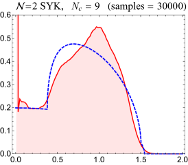
Figure 9: Spectral density of $M=Q+\overline{Q}$ in the ${\cal N}=2$ SYK model from exact diagonalization for $N_{c}=9$ and 10, averaged over random samples. Since the spectra are symmetric about $0$, only the nonnegative part is shown. The delta peaks at the origin represent exact zero modes, as in figure 6. In both plots $J=1$ and the total density is normalized to 1. The blue dashed lines are the best fits of analytic approximations based on the Marčenko-Pastur law.

The quality of the agreement is worse than for the previous model (figure 6). In particular, the pronounced sharp peak of the density cannot be reproduced with the Marčenko-Pastur law. This could be an indication that the ${\cal N}=2$ SYK model indeed has a more complex structure than the model in section 5.

In figure 9 there is a spectral gap for $N_{c}=9$ but not for $N_{c}=10$. The peculiar dependence of the level density of $H$ on the parity of $N_{c}$ was also noted in Stanford:2017thb . Intriguingly, this can easily be accounted for by the fact that a chiral block with $\overline{D}_{f}=\overline{D}_{f+3}$ is present only for odd $N_{c}$ (cf. appendix A). This can be shown by elementary combinatorics.

Symmetry of $M$

To classify $M$ based on RMT we can again make use of $P$ and $R\equiv P(-1)^{F}$ in the same way as for the ${\cal N}=1$ SYK model (section 4). For $N_{c}=1$ (mod 4), it can easily be shown that $P$ and $R$ map $\overline{V}_{f}\oplus\overline{V}_{f+3}$ to itself, with $f=\scalebox{0.8}{$\displaystyle\left\{\begin{array}[]{c}2\\ 1\\ 0\end{array}\right\}$}$ for $N_{c}=\scalebox{0.8}{$\displaystyle\left\{\begin{array}[]{c}1\\ 5\\ 9\end{array}\right\}$}$ (mod 12). Using (29) one can show

$$P^{2}=+1\,,\quad R^{2}=-1\,,\quad[R,M]=0\,,\quad\text{and}\quad\{P,M\}=0\,,$$ (33)

so $M$ on the corresponding space $\overline{V}_{f}\oplus\overline{V}_{f+3}$ is classified as class BdG (DIII) with $\beta=4$, according to table 1. Therefore every eigenvalue of $M$ must be twofold degenerate. On the other hand, with elementary combinatorics, one can show that $\overline{D}_{f}=\overline{D}_{f+3}=(2^{N_{c}-1}-1)/3\equiv d_{\text{odd}}$ (cf. appendix A) for the three sets of $f$ and $N_{c}$ specified above. The point is that $d_{\text{odd}}$ is an odd integer. This means that the spectrum of $M$ on $\overline{V}_{f}\oplus\overline{V}_{f+3}$ cannot consist of $d_{\text{odd}}$ positive levels and $d_{\text{odd}}$ negative levels, since this would contradict the Kramers degeneracy. We conclude that $M$ (and $H$) must have at least 2 zero modes in $\overline{V}_{f}\oplus\overline{V}_{f+3}$. This explains why we encounter “exceptional” zero modes for $N_{c}=1$ (mod 4), and is corroborated by our exact diagonalization analysis of $H$ (see appendix B).

It turns out, however, that the current approach is incapable of describing the actual level structure of $M$ in full detail. For instance, although $M$ in the sector $\overline{V}_{0}\oplus\overline{V}_{3}$ with $N_{c}=12$ is classified as class chGOE (BDI)_β=1, exact diagonalization shows that all nonzero eigenvalues of $M$ in this sector are in fact twofold degenerate. The reason that the symmetry classification based on $M$ is doomed to be incomplete is that $M$ does not manifestly reflect the fermion-number conservation of $H$. We have no access to the level statistics in the individual eigenspaces $V_{f}$ of $F$ as long as we see $H$ through the lens of $M$. The upshot is that since the structure of the ${\cal N}=2$ SYK model is qualitatively different from its cousins with ${\cal N}=0$ and 1 SUSY, we need an entirely new approach to carry out its symmetry classification. This is the subject of the next subsection.

6.3 Complete classification based on $Q\overline{Q}$ and $\overline{Q}Q$

Using the nilpotency $Q^{2}=\overline{Q}^{2}=0$ one can show that $H$, $Q\overline{Q}$, $\overline{Q}Q$ and $F$ all commute with one another, so they can be diagonalized simultaneously. Let $\psi$ be an eigenstate with $Q\overline{Q}\psi=\lambda_{+}\psi$ and $\overline{Q}Q\psi=\lambda_{-}\psi$ with $\lambda_{+}$, $\lambda_{-}\geq 0$. Let us assume $\lambda_{+}>0$ and $\lambda_{-}>0$. Then

$$\begin{split}\psi^{\dagger}\psi&=\frac{1}{\lambda_{+}\lambda_{-}}(\lambda_{+}\psi)^{\dagger}\lambda_{-}\psi=\frac{1}{\lambda_{+}\lambda_{-}}(Q\overline{Q}\psi)^{\dagger}\overline{Q}Q\psi\\ &=\frac{1}{\lambda_{+}\lambda_{-}}\psi^{\dagger}Q\overline{Q}^{2}Q\psi=0\,,\qquad(\because\,\overline{Q}^{2}=0)\end{split}$$ (34)

implying $\psi$ is a null vector. To resolve this contradiction, $\lambda_{+}=0$ or $\lambda_{-}=0$ must hold for every eigenstate. Note that $\lambda_{+}=0$ ($\lambda_{-}=0$) is equivalent to $\overline{Q}\psi=0$ ($Q\psi=0$) since, e.g., $Q\overline{Q}\psi=0$ implies $\psi^{\dagger}Q\overline{Q}\psi=||\overline{Q}\psi||^{2}=0$. If $\lambda_{+}=\lambda_{-}=0$, then $\psi$ is a zero mode (ground state) of $H$. Thus each subspace $V_{f}$ of $V$ for given $N_{c}$ admits an orthogonal decomposition

$$V_{f}=V_{f}^{+}\oplus V_{f}^{-}\oplus V_{f}^{z}\,,$$ (35)

where

$$V_{f}^{+} =\text{Hilbert space spanned by eigenstates $\psi$ with $\overline{Q}\psi\neq 0$ and $Q\psi=0$}\,,$$

$$V_{f}^{-} =\text{Hilbert space spanned by eigenstates $\psi$ with $\overline{Q}\psi=0$ and $Q\psi\neq 0$}\,,$$ (36)

$$V_{f}^{z} =\text{Hilbert space spanned by zero modes ($Q\psi=\overline{Q}\psi=0$)}\,.$$

(In figure 11 below we will show a graphical representation of the interrelations of the $V_{f}^{\pm,z}$.) Next we introduce notation for the dimensions of the subspaces,

$$\begin{split}N_{f}^{+}&\equiv\dim(V_{f}^{+})\,,\quad N_{f}^{-}\equiv\dim(V_{f}^{-})\,,\quad N_{f}^{z}\equiv\dim(V_{f}^{z})\,,\\ N_{f}&\equiv\dim(V_{f})=N_{f}^{+}+N_{f}^{-}+N_{f}^{z}=\binom{N_{c}}{f}\,,\quad N^{z}=\sum_{f=0}^{N_{c}}N_{f}^{z}\,.\end{split}$$ (37)

We choose to keep the $N_{c}$-dependence of $N_{f}^{\pm,z}$ implicit to avoid cluttering the notation. Using the properties (29) related to $P$ one can verify

$$N_{f}^{+}=N_{N_{c}-f}^{-}\,,\quad N_{f}^{-}=N_{N_{c}-f}^{+}\,,\quad N_{f}^{z}=N_{N_{c}-f}^{z}\,.$$ (38)

There is yet another important formula for $N_{f}^{\pm}$ . To derive it, we note that there is a one-to-one mapping between the bases of $V_{f}^{+}$ and those of $V_{f+3}^{-}$. Namely, if $\psi\in V_{f}^{+}$ with $Q\overline{Q}\psi=\lambda\psi$ for $\lambda>0$, then $\psi^{\prime}\equiv\frac{1}{\sqrt{\lambda}}\overline{Q}\psi\in V_{f+3}^{-}$ with $\overline{Q}Q\psi^{\prime}=\lambda\psi^{\prime}$. This can be inverted to give $\psi=\frac{1}{\sqrt{\lambda}}Q\psi^{\prime}$. Hence

$$\left.\begin{array}[]{rl}\overline{Q}(V_{f}^{+})&=V_{f+3}^{-}\\ Q(V_{f+3}^{-})&=V_{f}^{+}\end{array}\right\}~{}\text{for}\;\;0\leq f\leq N_{c}-3\quad\text{and}\quad N_{f}^{+}=N_{f+3}^{-}\,.$$ (41)

For convenience we provide tables of the numerical values of $N_{f}^{\pm,z}$ for $3\leq N_{c}\leq 17$ in appendix B. They confirm the relations (38) and (41). Explicit analytical formulas for $N_{f}^{\pm,z}$ will be derived in section 6.4.

This concludes the necessary preparations for the ensuing analysis. Our strategy in what follows is determined by the observation that $H$ is the sum of two operators that commute with each other. Therefore we need to classify the symmetries of $H$ on $V_{f}^{+}$ and $V_{f}^{-}$ separately. It is essential to distinguish these eigenspaces because they are not mixed by $H$ and the eigenvalues of $H$ on them are, a priori, statistically uncorrelated. Naïvely collecting all eigenvalues of $H$ on $V_{f}$ leads to incorrect statistics and must be avoided.

For generic $f$ and $N_{c}$ , there is no antiunitary symmetry that acts within $V_{f}^{\pm}$. $P$ just exchanges $V_{f}^{+}$ and $V_{N_{c}-f}^{-}$ (as well as $V_{f}^{-}$ and $V_{N_{c}-f}^{+}$), which does not impose constraints on the level statistics in any of the $V_{f}^{\pm}$. Therefore the symmetry class of $H$ on $V_{f}^{\pm}$ is generally GUE.

However, when the difference of $f$ and $N_{c}-f$ is $3$, there exists an antiunitary operator that commutes with $H$ and maps $V_{f}^{\pm}$ to itself. To see this, assume $f+3=N_{c}-f$ and let $\psi$ be a basis element of $V_{f}^{+}$ (so that $Q\overline{Q}\psi=\lambda\psi$ for some $\lambda>0$). Then $\overline{Q}\psi\in V_{f+3}^{-}$, cf. (41), and $P\overline{Q}\psi\in V^{+}_{f}$, so $P\overline{Q}$ is an antilinear operator that acts within $V_{f}^{+}$. By the same token one can show that $PQ$ maps $V_{f+3}^{-}$ to itself. The presence of these operators indicates that the spectra of $H$ on $V_{f}^{+}$ and $V_{f+3}^{-}$ in the case $f+3=N_{c}-f$ belong to either GOE or GSE. If we define the canonically normalized operators $P\overline{Q}/\sqrt{H}$ on $V^{+}_{f}$ and $PQ/\sqrt{H}$ on $V^{-}_{f+3}$ , one can show with the help of (29) that they are antiunitary and that their squares are $\pm 1$, depending on $N_{c}$ (mod 4). This sign determines the symmetry class (GOE/GSE). Our conclusions for the ${\cal N}=2$ SYK model with ${\hat{q}}=3$ are summarized in the following table.

(53)

This is the main result of this section. We have verified our classification by extensive numerical analysis of the spectra of $H$ projected to each $V_{f}$. The numerical results shown in figure 10 demonstrate excellent agreement with the RMT statistics specified in (53). Thus, as far as one can judge from the short-range correlations of energy levels, the ${\cal N}=2$ SYK model exhibits quantum chaos in each eigenspace of $F$ to the same extent as its ${\cal N}=0$ and 1 cousins.

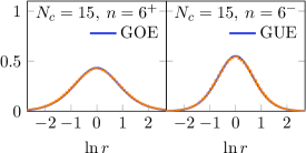
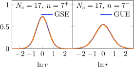
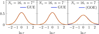
Figure 10: Distribution of the ratio $r$ of two consecutive level spacings for the ${\cal N}=2$ SYK model with ${\hat{q}}=3$. The label $n=f^{\pm}$ $(f=6,7)$ refers to levels of $H$ on $V_{f}^{\pm}$. The number of realizations used for averaging is $10^{3}$ for $N_{c}=15$ and $10^{2}$ for $N_{c}=16$ and $17$. The blue lines are surmises for the RMT classes of (53). The twofold degeneracy for the GSE case was resolved before the statistical analysis. In the right-most plot of $N_{c}=16$ we show the result obtained by an incorrect analysis, when levels from $V_{f}^{+}$ and $V_{f}^{-}$ are mixed into a single sequence. Although the result is surprisingly well fitted by the GOE, this is misleading: there is no antiunitary symmetry in this sector. This highlights the danger of inferring the symmetry class from spectra on the full $V_{f}$.

The argument above also clarifies the degeneracy of individual levels of $H$ when diagonalized on the whole Hilbert space $V$. In summary, we have found the following:

For $N_{c}=0,1,2$ (mod 4), every positive eigenvalue of $H$ is 4-fold degenerate. A quadruplet is formed by the set of eigenstates

$$\psi\in V_{f}^{+},\quad\overline{Q}\psi\in V_{f+3}^{-},\quad P\psi\in V_{N_{c}-f}^{-}\,,\quad\text{and}\quad P\overline{Q}\psi\in V_{N_{c}-f-3}^{+}$$ (54)

for $0\leq f\leq N_{c}-3$ . The number of quadruplets is $(2^{N_{c}}-N^{z})/4$. In particular, for even $N_{c}$ , every positive eigenvalue of $H$ on $V_{N_{c}/2}$ is twofold degenerate, because both $\psi$ and $P\psi\in V_{N_{c}/2}$ .

For $N_{c}=3$ (mod 4), there are $N_{\scriptscriptstyle(N_{c}-3)/2}^{+}\,(=N_{\scriptscriptstyle(N_{c}+3)/2}^{-})$ doublets residing in the GOE sectors and $(2^{N_{c}}-N^{z}-2N_{\scriptscriptstyle(N_{c}-3)/2}^{+})/4$ quadruplets. The latter consist of the set (54) subject to the condition that $f\neq(N_{c}-3)/2$.

6.4 Analytical formulas for $N_{f}^{\pm}$ and $N_{f}^{z}$

Up to now we have not mentioned how to compute $N_{f}^{\pm}$ explicitly for given $f$ and $N_{c}$ . Actually this proves to be a straightforward (albeit tedious) task if we posit the following premise:

For any $$N_{c}\geq 3 H V_{f} |f-N_{c}/2|\leq 3/2 N_{c}=1$$, all exact zero modes of reside in with , where the equality holds only for exceptional zero modes that occur when (mod 4). (55)

This rather strong condition on the ground states of $H$ is not only corroborated by detailed numerical simulations (see appendix B and Fu:2016vas ) but also derived from the Schwarzian effective theory valid in the large-$N_{c}$ and low-energy limit Stanford:2017thb ; Mertens:2017mtv . If (55) is accepted, one can fully clarify the relation of Hilbert spaces linked by $\overline{Q}$ as in table 8. The sequences tabulated there are exact sequences in the terminology of mathematics, in the sense that the kernel of $\overline{Q}$ acting on $V_{f}$ coincides exactly with the image of $V_{f-3}$ by $\overline{Q}$. Two examples of these sequences, extended up to $V_{N_{c}}$, are graphically illustrated in figure 11 for $N_{c}=15$.

Table 8: Exact sequences of the Hilbert spaces generated by the linear map $\overline{Q}$. Complementary exact sequences descending from $V_{N_{c}}$, $V_{N_{c}-1}$, and $V_{N_{c}-2}$ by way of $Q$ can be obtained by applying the particle-hole operator $P$ to the sequences in the table. The spaces ${\color[rgb]{1,0,0}V}$ contain an exponentially large number of “typical” zero modes, see (32). The spaces ${\color[rgb]{0,0,1}V^{*}}$ contain no zero modes for $N_{c}=3$ (mod 4), or $1$ or $3$ “exceptional” zero modes for $N_{c}=1$ (mod 4).

​​​​$\begin{array}[]{c}N_{c}\vspace{-5pt}\\ \text{\footnotesize(mod~{}6)}\end{array}$​​​​	Exact Sequence	​​​​$\begin{array}[]{c}N_{c}\vspace{-5pt}\\ \text{\footnotesize(mod~{}6)}\end{array}$​​​​	Exact Sequence
0	$\displaystyle\begin{array}[]{l}V_{0}\xrightarrow{\overline{Q}}V_{3}\xrightarrow{\overline{Q}}\cdots\xrightarrow{\overline{Q}}{\color[rgb]{1,0,0}V_{N_{c}/2}}\\ V_{1}\xrightarrow{\overline{Q}}V_{4}\xrightarrow{\overline{Q}}\cdots\xrightarrow{\overline{Q}}{\color[rgb]{1,0,0}V_{N_{c}/2+1}}\\ V_{2}\xrightarrow{\overline{Q}}V_{5}\xrightarrow{\overline{Q}}\cdots\xrightarrow{\overline{Q}}{\color[rgb]{1,0,0}V_{N_{c}/2-1}}\end{array}$	3	$\displaystyle\begin{array}[]{l}V_{0}\xrightarrow{\overline{Q}}V_{3}\xrightarrow{\overline{Q}}\cdots\xrightarrow{\overline{Q}}{\color[rgb]{0,0,1}V_{(N_{c}-3)/2}^{*}}\\ V_{1}\xrightarrow{\overline{Q}}V_{4}\xrightarrow{\overline{Q}}\cdots\xrightarrow{\overline{Q}}{\color[rgb]{1,0,0}V_{(N_{c}-1)/2}}\\ V_{2}\xrightarrow{\overline{Q}}V_{5}\xrightarrow{\overline{Q}}\cdots\xrightarrow{\overline{Q}}{\color[rgb]{1,0,0}V_{(N_{c}+1)/2}}\raisebox{-7.0pt}{}\end{array}$
1	$\displaystyle\begin{array}[]{l}V_{0}\xrightarrow{\overline{Q}}V_{3}\xrightarrow{\overline{Q}}\cdots\xrightarrow{\overline{Q}}{\color[rgb]{1,0,0}V_{(N_{c}-1)/2}}\\ V_{1}\xrightarrow{\overline{Q}}V_{4}\xrightarrow{\overline{Q}}\cdots\xrightarrow{\overline{Q}}{\color[rgb]{1,0,0}V_{(N_{c}+1)/2}}\\ V_{2}\xrightarrow{\overline{Q}}V_{5}\xrightarrow{\overline{Q}}\cdots\xrightarrow{\overline{Q}}{\color[rgb]{0,0,1}V_{(N_{c}-3)/2}^{*}}\end{array}$	4	$\displaystyle\begin{array}[]{l}V_{0}\xrightarrow{\overline{Q}}V_{3}\xrightarrow{\overline{Q}}\cdots\xrightarrow{\overline{Q}}{\color[rgb]{1,0,0}V_{N_{c}/2+1}}\\ V_{1}\xrightarrow{\overline{Q}}V_{4}\xrightarrow{\overline{Q}}\cdots\xrightarrow{\overline{Q}}{\color[rgb]{1,0,0}V_{N_{c}/2-1}}\\ V_{2}\xrightarrow{\overline{Q}}V_{5}\xrightarrow{\overline{Q}}\cdots\xrightarrow{\overline{Q}}{\color[rgb]{1,0,0}V_{N_{c}/2}}\raisebox{-7.0pt}{}\end{array}$
2	$\displaystyle\begin{array}[]{l}V_{0}\xrightarrow{\overline{Q}}V_{3}\xrightarrow{\overline{Q}}\cdots\xrightarrow{\overline{Q}}{\color[rgb]{1,0,0}V_{N_{c}/2-1}}\\ V_{1}\xrightarrow{\overline{Q}}V_{4}\xrightarrow{\overline{Q}}\cdots\xrightarrow{\overline{Q}}{\color[rgb]{1,0,0}V_{N_{c}/2}}\\ V_{2}\xrightarrow{\overline{Q}}V_{5}\xrightarrow{\overline{Q}}\cdots\xrightarrow{\overline{Q}}{\color[rgb]{1,0,0}V_{N_{c}/2+1}}\end{array}$	5	$\displaystyle\begin{array}[]{l}V_{0}\xrightarrow{\overline{Q}}V_{3}\xrightarrow{\overline{Q}}\cdots\xrightarrow{\overline{Q}}{\color[rgb]{1,0,0}V_{(N_{c}+1)/2}}\\ V_{1}\xrightarrow{\overline{Q}}V_{4}\xrightarrow{\overline{Q}}\cdots\xrightarrow{\overline{Q}}{\color[rgb]{0,0,1}V_{(N_{c}-3)/2}^{*}}\\ V_{2}\xrightarrow{\overline{Q}}V_{5}\xrightarrow{\overline{Q}}\cdots\xrightarrow{\overline{Q}}{\color[rgb]{1,0,0}V_{(N_{c}-1)/2}}\raisebox{-7.0pt}{}\end{array}$

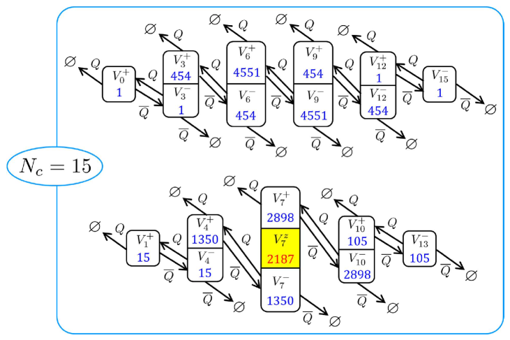
Figure 11: Relations among the Hilbert spaces with $F=0$ and $1$ (mod 3) for $N_{c}=15$. The numbers shown are the dimensions of the corresponding subspaces of $V$. Arrows to the symbol $\varnothing$ (empty set) are shown to emphasize the nilpotency $Q^{2}={\overline{Q}}^{2}=0$.

Although we do not provide a rigorous proof of (55), there is a heuristic argument to convince oneself that (55) is correct. Let us consider a sequence $\cdots\xrightarrow{\overline{Q}}V_{f}\xrightarrow{\overline{Q}}V_{f+3}\xrightarrow{\overline{Q}}\cdots$ with $\dim(V_{f})<\dim(V_{f+3})$. If $\overline{Q}$ in the middle were a completely random linear map, it is a matrix of size $\dim(V_{f})\times\dim(V_{f+3})$ whose rank is almost surely $\dim(V_{f})$ (in the absence of fine-tuning or a special symmetry). This is of course an oversimplification for $\overline{Q}$, because it is not a generic linear map but a nilpotent map. Taking this into account, let us next view $\overline{Q}$ as a random matrix of size $\dim\big{[}V_{f}\setminus\overline{Q}(V_{f-3})\big{]}\times\dim(V_{f+3})$, where the trivial kernel $\overline{Q}(V_{f-3})$ has been left out. Then the rank of $\overline{Q}$ is almost surely $\dim\big{[}V_{f}\setminus\overline{Q}(V_{f-3})\big{]}$, i.e., there is no “nontrivial” zero mode of $\overline{Q}$ in $V_{f}$. This argument may be repeated along the sequence as long as the condition $\dim(V_{f})<\dim(V_{f+3})$ is fulfilled. A completely parallel argument can also be given for a “descending” sequence $\cdots\xleftarrow{Q}V_{f}\xleftarrow{Q}V_{f+3}\xleftarrow{Q}\cdots$ with $\dim(V_{f})>\dim(V_{f+3})$. By pinching the sequence from both ends like this, we find at the end of the day that all zero modes $(Q\psi=\overline{Q}\psi=0)$ must be concentrated in the subspace $V_{f}$ with the largest dimension in the sequence. This is equivalent to the condition (55).

Now it is straightforward to work out $N_{f}^{\pm}$. Let us begin with the case of even $N_{c}$ . First, for $3\leq f<N_{c}/2-1$, $V_{f}$ does not contain zero modes under the assumption (55). Hence, with the help of (41), we find

$$N_{f}^{+}=\binom{N_{c}}{f}-N_{f}^{-}=\binom{N_{c}}{f}-N_{f-3}^{+}\,.$$ (56)

This recursion relation for $N_{f}^{+}$ is to be solved with the initial conditions $N_{0}^{+}=1$, $N_{1}^{+}=N_{c}$, and $N_{2}^{+}=N_{c}(N_{c}-1)/2$. The result reads

$$N_{f}^{+} =N_{N_{c}-f}^{-}=(-1)^{f+f_{0}}N_{f_{0}}^{+}+(-1)^{f}\sum_{n=1}^{(f-f_{0})/3}(-1)^{3n+f_{0}}\binom{N_{c}}{3n+f_{0}}\,,$$ (57)

$$N_{f}^{-} =N_{N_{c}-f}^{+}=\binom{N_{c}}{f}-N_{f}^{+}\,,$$ (58)

where $f_{0}\equiv f-3\lfloor f/3\rfloor\in\{0,1,2\}$. Equation (38) was used in the first equalities of (57) and (58). These formulas hold in the range $0\leq f<N_{c}/2-1$. We verified (57) numerically for $N_{c}$ up to $17$.

Finally, to derive $N_{f}^{\pm}$ for $f$ close to $N_{c}/2$ , we need to know $N_{f}^{z}$ . Recalling the premise (55) and the fact that the inequality (32) is saturated except when $N_{c}=1$ (mod 4) (see appendix A for $\overline{D}_{f}$ and section 6.2 for the origin of the $1$ or $3$ “exceptional” zero modes in this case), we readily arrive at the following summary:

(70)

which fully agrees with numerical results in Fu:2016vas . This input should be plugged into

$$N^{+}_{f}=\binom{N_{c}}{f}-N^{+}_{f-3}-N_{f}^{z}\quad\text{and}\quad N_{f}^{-}=N_{f-3}^{+}\qquad\text{for}\quad f=\frac{N_{c}}{2},\,\frac{N_{c}}{2}\pm 1\,,$$ (71)

where $N^{+}_{f-3}$ has been obtained by (57). This completes our discussion of even $N_{c}$ .

For odd $N_{c}$, (57) and (58) still hold in the range $0\leq f<(N_{c}-3)/2$ (see table 8). For $f$ near $N_{c}/2$ we only have to substitute (70) into

$$N^{+}_{f}=\binom{N_{c}}{f}-N^{+}_{f-3}-N_{f}^{z}\quad\text{and}\quad N_{f}^{-}=N_{f-3}^{+}\qquad\text{for}\quad f=\frac{N_{c}\pm 1}{2},\,\frac{N_{c}\pm 3}{2}\,.$$ (72)

The numerical results in appendix B agree with the formulas derived in this subsection.

6.5 Generalization to ${\hat{q}}>3$

We now generalize the preceding classification scheme to the ${\cal N}=2$ SYK model with $H=\{Q,\overline{Q}\}$ and ${\hat{q}}$ complex fermions in the supercharge, where ${\hat{q}}$ is odd, i.e.,

$$Q=i^{({\hat{q}}-1)/2}\!\!\!\!\!\!\!\!\!\sum_{1\leq i_{1}<\cdots<i_{{\hat{q}}}\leq N_{c}}\!\!\!\!\!X_{i_{1}i_{2}\cdots i_{{\hat{q}}}}c_{i_{1}}c_{i_{2}}\cdots c_{i_{\hat{q}}}\quad\text{and}\quad\overline{Q}=i^{({\hat{q}}-1)/2}\!\!\!\!\!\!\!\!\!\sum_{1\leq i_{1}<\cdots<i_{{\hat{q}}}\leq N_{c}}\!\!\!\!\!\overline{X_{i_{1}i_{2}\cdots i_{{\hat{q}}}}}\overline{c}_{i_{1}}\overline{c}_{i_{2}}\cdots\overline{c}_{i_{\hat{q}}}\,.$$ (73)

This is a counterpart of (9) with ${\cal N}=1$. For ${\hat{q}}=3$ it reverts to (21). The tables (29) and (53) for ${\hat{q}}=3$ are now generalized to

(85)

and

(111)

respectively. We numerically tested this table via exact diagonalization of $H$. Figure 12 shows superb agreement between the numerical data and RMT.

We also analyzed the dimensions $N_{f}^{\pm,z}$ of the subspaces, for which formulas similar to those in section 6.4 can be derived. For ${\hat{q}}=5$, we have numerically confirmed up to $N_{c}=17$ that all exact zero modes of $H$ reside in $V_{f}$ with $|f-N_{c}/2|\leq 5/2$. The last inequality is saturated only for $N_{c}=7$ and $11$ by just 2 zero modes in each case. This is not only consistent with our heuristic argument in section 6.4 but also conforms to the claim at large $N_{c}$ Stanford:2017thb ; Mertens:2017mtv that all zero modes should satisfy $|f-N_{c}/2|<{\hat{q}}/2$. In the regime $N_{c}\gg 1$ one can ignore $\mathcal{O}(1)$ exceptional zero modes and the strict inequality may be justified.

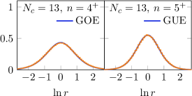
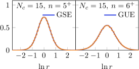
Figure 12: Same as figure 10 but for ${\hat{q}}=5$ and compared with the surmises of the RMT classes in table (111). The number of realizations used for averaging is $10^{3}$ for $N_{c}=13$ and $10^{2}$ for $N_{c}=15$.

7 Conclusions

In this paper we have completed the symmetry classification of SYK models with ${\cal N}=0$, 1, and 2 SUSY on the basis of the Altland-Zirnbauer theory of random matrices (table 1). The symmetry classes of RMT not only tell us the level degeneracies of the Hamiltonian but also offer a diagnostic tool of quantum chaos through level correlations in the bulk of the spectrum. Furthermore, when the spectral mirror symmetry is present, RMT precisely predicts universal level correlation functions in the vicinity of the origin (also known as hard edge or microscopic domain Verbaarschot:2000dy ). The present work can be viewed as a generalization of preceding works You:2016ldz ; Garcia-Garcia:2016mno ; Cotler:2016fpe ; Garcia-Garcia:2017pzl ; Li:2017hdt that analyzed the level statistics of the ${\cal N}=0$ and $1$ SYK models solely with a 4-body interaction. Our new results include the following:

1. The symmetry classification of the ${\cal N}=0$ SYK model was given for a Hamiltonian with the most generic $q$-body interaction. The result, summarized in tables 2 and 3, includes the RMT classes C and D that did not show up in the preceding classification of You:2016ldz ; Garcia-Garcia:2016mno ; Cotler:2016fpe ; Garcia-Garcia:2017pzl ; Li:2017hdt . Our results were corroborated by detailed numerics (figure 1).

2. We numerically compared the smallest eigenvalue distributions in the ${\cal N}=0$ SYK model with $q=6$ with the RMT predictions of class C and D, finding excellent agreement (figure 2).

3. The symmetry classification of the ${\cal N}=1$ SYK model was given for a supercharge with the most generic interaction of ${\hat{q}}$ Majorana fermions (tables 4 and 5). This extends Li:2017hdt which investigated only ${\hat{q}}=3$. Our results were corroborated by detailed numerics (figure 3).

4. We numerically compared the smallest eigenvalue distributions in the ${\cal N}=1$ SYK model with ${\hat{q}}=3$ and $5$ with the RMT predictions, finding excellent agreement (figures 4 and 5). This confirms the hard-edge universality of the ${\cal N}=1$ SYK model for the first time and is relevant for the thermodynamics of this model at low temperatures comparable to the energy scale of the SUSY breaking.

5. We proposed an intriguing new SYK-type model which lacks SUSY but whose Hamiltonian is semi-positive definite and has an extensive number of zero-energy states (section 5). The symmetry classification based on RMT was provided, and a detailed numerical analysis of the spectra both in the bulk and near the origin was performed, resulting in agreement with the RMT predictions.

6. We completed the RMT classification of the ${\cal N}=2$ SYK model for the first time. This model is qualitatively different from its ${\cal N}=0$ and $1$ cousins in various aspects. It is a model of complex fermions rather than Majorana fermions, and it has a $\text{U}(1)$ R-symmetry. The symmetry classification of this model is nontrivial because the structure of its Hilbert space is far more complex (see figure 11 for an example) than that of the ${\cal N}=0$ SYK model with complex fermions considered previously in Sachdev:2015efa ; You:2016ldz ; Fu:2016yrv ; Davison:2016ngz ; Bulycheva2017 . Our main results, summarized in table (53) for ${\hat{q}}=3$ and in table (111) for general odd ${\hat{q}}$, are strongly supported by intensive numerics, as shown in figure 10 (for ${\hat{q}}=3$) and figure 12 (for ${\hat{q}}=5$).

7. In section 6.2 we succeeded in giving a logical explanation for the curious fact Fu:2016vas ; Sannomiya:2016mnj that, in the ${\cal N}=2$ SYK model, the number of zero-energy ground states exactly agrees with the lower bound from the Witten index in some cases but not in other cases. In short, this is due to the dichotomy between the odd dimensionality of the Hilbert space and Kramers degeneracy.

This work can be extended in several directions. First, our analysis of spectral properties of the Hamiltonian could be further deepened by using probes that are sensitive to long-range correlations of energy levels, like the level number variance $\Sigma^{2}(L)$ and the spectral rigidity $\Delta_{3}(L)$ Guhr:1997ve ; Mehta_book . Investigating the spectral form factor of the ${\cal N}=2$ SYK model and making a quantitative comparison with RMT along the lines of Cotler:2016fpe is another future direction, although physical interpretation of the ramp, dip, etc., of the spectral form factor as a signature of quantum chaos is rather subtle Balasubramanian:2016ids . Finally, we note that there is no analytical result for the global spectral density of the ${\cal N}=1$ and $2$ SYK models, although an accurate formula is already known for the ${\cal N}=0$ model Garcia-Garcia:2016mno ; Cotler:2016fpe ; Garcia-Garcia:2017pzl . We wish to address some of these problems in the future.

Appendix A $\overline{D}_{f}$ in the ${\cal N}=2$ SYK model

In this appendix we display short convenient expressions for $\overline{D}_{f}$ as defined in (31) for the ${\cal N}=2$ SYK model with ${\hat{q}}=3$. For simplicity we denote $N_{c}$ by $N$ in this appendix. Then

$$\overline{D}_{0} =\frac{1}{6}\left[2^{N}+2\cdot 3^{N/2}\cos{\frac{N\pi}{6}}+2\cos{\frac{N\pi}{3}}\right],$$ (112)

$$\overline{D}_{1} =\frac{1}{6}\left[2^{N}-2\cdot 3^{N/2}\cos{\frac{(N+4)\pi}{6}}+2\cos{\frac{(N-2)\pi}{3}}\right],$$ (113)

$$\overline{D}_{2} =\frac{1}{6}\left[2^{N}+2\cdot 3^{N/2}\cos{\frac{(N-4)\pi}{6}}+2\cos{\frac{(N+2)\pi}{3}}\right],$$ (114)

$$\overline{D}_{3} =\frac{1}{6}\left[2^{N}-2\cdot 3^{N/2}\cos{\frac{N\pi}{6}}+2\cos{\frac{N\pi}{3}}\right],$$ (115)

$$\overline{D}_{4} =\frac{1}{6}\left[2^{N}+2\cdot 3^{N/2}\cos{\frac{(N+4)\pi}{6}}+2\cos{\frac{(N-2)\pi}{3}}\right],$$ (116)

$$\overline{D}_{5} =\frac{1}{6}\left[2^{N}-2\cdot 3^{N/2}\cos{\frac{(N-4)\pi}{6}}+2\cos{\frac{(N+2)\pi}{3}}\right].$$ (117)

Appendix B Dimensions of Hilbert spaces for ${\cal N}=2$

In this appendix we present tables of the $N_{f}^{\pm,z}$ defined in (37) for the ${\cal N}=2$ SYK model with ${\hat{q}}=3$, for $N_{c}=3,4,\dots,17$. The symmetry classes are  ​​​ : GOE,  ​​​ : GSE, and uncolored numbers GUE. All of these results were checked numerically.

$\blacksquare$ $N_{c}=3$

  $f$ 0 1 2 3 $N_{f}^{+}$ 1 0 0 0 $N_{f}^{-}$ 0 0 0 1 $N_{f}^{z}$ 0 3 3 0

$\blacksquare$ $N_{c}=4$

  $f$ 0 1 2 3 4 $N_{f}^{+}$ 1 1 0 0 0 $N_{f}^{-}$ 0 0 0 1 1 $N_{f}^{z}$ 0 3 6 3 0

$\blacksquare$ $N_{c}=5$

  $f$ 0 1 2 3 4 5 $N_{f}^{+}$ 1 4 1 0 0 0 $N_{f}^{-}$ 0 0 0 1 4 1 $N_{f}^{z}$ 0 1 9 9 1 0

$\blacksquare$ $N_{c}=6$

  $f$ 0 1 2 3 4 5 6 $N_{f}^{+}$ 1 6 6 1 0 0 0 $N_{f}^{-}$ 0 0 0 1 6 6 1 $N_{f}^{z}$ 0 0 9 18 9 0 0

$\blacksquare$ $N_{c}=7$

  $f$ 0 1 2 3 4 5 6 7 $N_{f}^{+}$ 1 7 21 7 1 0 0 0 $N_{f}^{-}$ 0 0 0 1 7 21 7 1 $N_{f}^{z}$ 0 0 0 27 27 0 0 0

$\blacksquare$ $N_{c}=8$

  $f$ 0 1 2 3 4 5 6 7 8 $N_{f}^{+}$ 1 8 28 28 8 1 0 0 0 $N_{f}^{-}$ 0 0 0 1 8 28 28 8 1 $N_{f}^{z}$ 0 0 0 27 54 27 0 0 0

$\blacksquare$ $N_{c}=9$

  $f$ 0 1 2 3 4 5 6 7 8 9 $N_{f}^{+}$ 1 9 36 80 36 9 1 0 0 0 $N_{f}^{-}$ 0 0 0 1 9 36 80 36 9 1 $N_{f}^{z}$ 0 0 0 3 81 81 3 0 0 0

$\blacksquare$ $N_{c}=10$

  $f$ 0 1 2 3 4 5 6 7 8 9 10 $N_{f}^{+}$ 1 10 45 119 119 45 10 1 0 0 0 $N_{f}^{-}$ 0 0 0 1 10 45 119 119 45 10 1 $N_{f}^{z}$ 0 0 0 0 81 162 81 0 0 0 0

$\blacksquare$ $N_{c}=11$

  $f$ 0 1 2 3 4 5 6 7 8 9 10 11 $N_{f}^{+}$ 1 11 55 164 319 164 55 11 1 0 0 0 $N_{f}^{-}$ 0 0 0 1 11 55 164 319 164 55 11 1 $N_{f}^{z}$ 0 0 0 0 0 243 243 0 0 0 0 0

$\blacksquare$ $N_{c}=12$

  $f$ 0 1 2 3 4 5 6 7 8 9 10 11 12 $N_{f}^{+}$ 1 12 66 219 483 483 219 66 12 1 0 0 0 $N_{f}^{-}$ 0 0 0 1 12 66 219 483 483 219 66 12 1 $N_{f}^{z}$ 0 0 0 0 0 243 486 243 0 0 0 0 0

$\blacksquare$ $N_{c}=13$

  $f$ 0 1 2 3 4 5 6 7 8 9 10 11 12 13 $N_{f}^{+}$ 1 13 78 285 702 1208 702 285 78 13 1 0 0 0 $N_{f}^{-}$ 0 0 0 1 13 78 285 702 1208 702 285 78 13 1 $N_{f}^{z}$ 0 0 0 0 0 1 729 729 1 0 0 0 0 0

$\blacksquare$ $N_{c}=14$

  $f$ 0 1 2 3 4 5 6 7 8 9 10 11 12 13 14 $N_{f}^{+}$ 1 14 91 363 987 1911 1911 987 363 91 14 1 0 0 0 $N_{f}^{-}$ 0 0 0 1 14 91 363 987 1911 1911 987 363 91 14 1 $N_{f}^{z}$ 0 0 0 0 0 0 729 1458 729 0 0 0 0 0 0

$\blacksquare$ $N_{c}=15$

  $f$ 0 1 2 3 4 5 6 7 8 9 10 11 12 13 14 15 $N_{f}^{+}$ 1 15 105 454 1350 2898 4551 2898 1350 454 105 15 1 0 0 0 $N_{f}^{-}$ 0 0 0 1 15 105 454 1350 2898 4551 2898 1350 454 105 15 1 $N_{f}^{z}$ 0 0 0 0 0 0 0 2187 2187 0 0 0 0 0 0 0

$\blacksquare$ $N_{c}=16$

  $f$ 0 1 2 3 4 5 6 7 8 9 10 11 12 13 14 15 16 $N_{f}^{+}$ 1 16 120 559 1804 4248 7449 7449 4248 1804 559 120 16 1 0 0 0 $N_{f}^{-}$ 0 0 0 1 16 120 559 1804 4248 7449 7449 4248 1804 559 120 16 1 $N_{f}^{z}$ 0 0 0 0 0 0 0 2187 4374 2187 0 0 0 0 0 0 0

$\blacksquare$ $N_{c}=17$

  $f$ 0 1 2 3 4 5 6 7 8 9 10 11 12 13 14 15 16 17 $N_{f}^{+}$ 1 17 136 679 2363 6052 11697 17084 11697 6052 2363 679 136 17 1 0 0 0 $N_{f}^{-}$ 0 0 0 1 17 136 679 2363 6052 11697 17084 11697 6052 2363 679 136 17 1 $N_{f}^{z}$ 0 0 0 0 0 0 0 1 6561 6561 1 0 0 0 0 0 0 0

References

- (1) O. Bohigas, M. J. Giannoni and C. Schmit, Characterization of chaotic quantum spectra and universality of level fluctuation laws, Phys. Rev. Lett. 52 (1984) 1–4.
- (2) T. Guhr, A. Muller-Groeling and H. A. Weidenmuller, Random matrix theories in quantum physics: Common concepts, Phys. Rept. 299 (1998) 189–425, [cond-mat/9707301].
- (3) S. Müller, S. Heusler, A. Altland, P. Braun and F. Haake, Periodic-orbit theory of universal level correlations in quantum chaos, New J. Phys. 11 (2009) 103025, [0906.1960].
- (4) J. M. Deutsch, Quantum statistical mechanics in a closed system, Phys. Rev. A 43 (Feb, 1991) 2046–2049.
- (5) M. Srednicki, Chaos and Quantum Thermalization, Phys. Rev. E 50 (1994) 888, [cond-mat/9403051].
- (6) T. S. Biro, S. G. Matinyan and B. Muller, Chaos and gauge field theory, World Sci. Lect. Notes Phys. 56 (1994) 1–288.
- (7) H.-J. Stöckmann, Quantum Chaos: An Introduction. Cambridge University Press, Cambridge, 2007.
- (8) F. Haake, Quantum Signatures of Chaos. Springer, New York, 2010.
- (9) J. Gomez, K. Kar, V. Kota, R. Molina, A. Relano and J. Retamosa, Many-body quantum chaos: Recent developments and applications to nuclei, Phys. Rept. 499 (2011) 103 – 226.
- (10) C. Gogolin and J. Eisert, Equilibration, thermalisation, and the emergence of statistical mechanics in closed quantum systems, Rep. Prog. Phys. 79 (2016) 056001, [1503.07538].
- (11) L. D’Alessio, Y. Kafri, A. Polkovnikov and M. Rigol, From Quantum Chaos and Eigenstate Thermalization to Statistical Mechanics and Thermodynamics, Adv. Phys. 65 (2016) 239, [1509.06411].
- (12) Y. Sekino and L. Susskind, Fast Scramblers, JHEP 10 (2008) 065, [0808.2096].
- (13) S. Sachdev, Holographic metals and the fractionalized Fermi liquid, Phys. Rev. Lett. 105 (2010) 151602, [1006.3794].
- (14) L. Susskind, Addendum to Fast Scramblers, 1101.6048.
- (15) N. Lashkari, D. Stanford, M. Hastings, T. Osborne and P. Hayden, Towards the Fast Scrambling Conjecture, JHEP 04 (2013) 022, [1111.6580].
- (16) S. H. Shenker and D. Stanford, Black holes and the butterfly effect, JHEP 03 (2014) 067, [1306.0622].
- (17) S. H. Shenker and D. Stanford, Multiple Shocks, JHEP 12 (2014) 046, [1312.3296].
- (18) D. Harlow, Jerusalem Lectures on Black Holes and Quantum Information, Rev. Mod. Phys. 88 (2016) 15002, [1409.1231].
- (19) D. A. Roberts, D. Stanford and L. Susskind, Localized shocks, JHEP 03 (2015) 051, [1409.8180].
- (20) D. A. Roberts and D. Stanford, Diagnosing Chaos Using Four-Point Functions in Two-Dimensional Conformal Field Theory, Phys. Rev. Lett. 115 (2015) 131603, [1412.5123].
- (21) S. H. Shenker and D. Stanford, Stringy effects in scrambling, JHEP 05 (2015) 132, [1412.6087].
- (22) A. Larkin and Y. N. Ovchinnikov, Quasiclassical method in the theory of superconductivity, Sov. JETP 28 (1969) 1200.
-
(23)
A. Kitaev, Hidden correlations in the Hawking radiation and thermal
noise, https://www.youtube.com/watch?v=OQ9qN8j7EZI,
http://online.kitp.ucsb.edu/online/joint98/kitaev/.
Talk at 2015 Breakthrough Prize Fundamental Physics Symposium, Nov. 10, 2014 and Talk at KITP seminar, Feb. 12, 2015 . - (24) J. Maldacena, S. H. Shenker and D. Stanford, A bound on chaos, JHEP 08 (2016) 106, [1503.01409].
- (25) S. Sachdev and J. Ye, Gapless spin fluid ground state in a random, quantum Heisenberg magnet, Phys. Rev. Lett. 70 (1993) 3339, [cond-mat/9212030].
-
(26)
A. Kitaev, A simple model of quantum holography, http://online.kitp.ucsb.edu/online/entangled15/kitaev/,
http://online.kitp.ucsb.edu/online/entangled15/kitaev2/.
Talks at KITP, April 7, 2015 and May 27, 2015 . - (27) A. Georges, O. Parcollet and S. Sachdev, Mean Field Theory of a Quantum Heisenberg Spin Glass, Phys. Rev. Lett. 85 (2000) 840, [cond-mat/9909239].
- (28) A. Georges, O. Parcollet and S. Sachdev, Quantum Fluctuations of a Nearly Critical Heisenberg Spin Glass, Phys. Rev. B 63 (2001) 134406, [cond-mat/0009388].
- (29) S. Sachdev, Bekenstein-Hawking Entropy and Strange Metals, Phys. Rev. X5 (2015) 041025, [1506.05111].
- (30) J. Polchinski and V. Rosenhaus, The Spectrum in the Sachdev-Ye-Kitaev Model, JHEP 04 (2016) 001, [1601.06768].
- (31) J. Maldacena and D. Stanford, Remarks on the Sachdev-Ye-Kitaev model, Phys. Rev. D94 (2016) 106002, [1604.07818].
- (32) J. Maldacena, D. Stanford and Z. Yang, Conformal symmetry and its breaking in two dimensional Nearly Anti-de-Sitter space, PTEP 2016 (2016) 12C104, [1606.01857].
- (33) J. Engelsöy, T. G. Mertens and H. Verlinde, An investigation of AdS2 backreaction and holography, JHEP 07 (2016) 139, [1606.03438].
- (34) P. Hosur, X.-L. Qi, D. A. Roberts and B. Yoshida, Chaos in quantum channels, JHEP 02 (2016) 004, [1511.04021].
- (35) W. Fu and S. Sachdev, Numerical study of fermion and boson models with infinite-range random interactions, Phys. Rev. B94 (2016) 035135, [1603.05246].
- (36) D. A. Roberts and B. Swingle, Lieb-Robinson Bound and the Butterfly Effect in Quantum Field Theories, Phys. Rev. Lett. 117 (2016) 091602, [1603.09298].
- (37) K. Jensen, Chaos in AdS2 Holography, Phys. Rev. Lett. 117 (2016) 111601, [1605.06098].
- (38) D. Bagrets, A. Altland and A. Kamenev, Sachdev-Ye-Kitaev model as Liouville quantum mechanics, Nucl. Phys. B911 (2016) 191–205, [1607.00694].
- (39) E. B. Rozenbaum, S. Ganeshan and V. Galitski, Lyapunov Exponent and Out-of-Time-Ordered Correlator’s Growth Rate in a Chaotic System, Phys. Rev. Lett. 118 (2017) 086801, [1609.01707].
- (40) N. Tsuji, P. Werner and M. Ueda, Exact out-of-time-ordered correlation functions for an interacting lattice fermion model, Phys. Rev. A95 (2017) 011601, [1610.01251].
- (41) M. Berkooz, P. Narayan, M. Rozali and J. Simón, Higher Dimensional Generalizations of the SYK Model, JHEP 01 (2017) 138, [1610.02422].
- (42) D. A. Roberts and B. Yoshida, Chaos and complexity by design, JHEP 04 (2017) 121, [1610.04903].
- (43) A. A. Patel and S. Sachdev, Quantum chaos on a critical Fermi surface, Proc. Nat. Acad. Sci. 114 (2017) 1844–1849, [1611.00003].
- (44) R. A. Davison, W. Fu, A. Georges, Y. Gu, K. Jensen and S. Sachdev, Thermoelectric transport in disordered metals without quasiparticles: the SYK models and holography, Phys. Rev. B95 (2017) 155131, [1612.00849].
- (45) V. Balasubramanian, B. Craps, B. Czech and G. Sarosi, Echoes of chaos from string theory black holes, JHEP 03 (2017) 154, [1612.04334].
- (46) Y. Liu, M. A. Nowak and I. Zahed, Disorder in the Sachdev-Yee-Kitaev Model, 1612.05233.
- (47) D. Bagrets, A. Altland and A. Kamenev, Power-law out of time order correlation functions in the SYK model, Nucl. Phys. B921 (2017) 727–752, [1702.08902].
- (48) D. Chowdhury and B. Swingle, Onset of many-body chaos in the model, 1703.02545.
- (49) K. Hashimoto, K. Murata and R. Yoshii, Out-of-time-order correlators in quantum mechanics, 1703.09435.
- (50) E. Witten, An SYK-Like Model Without Disorder, 1610.09758.
- (51) S. Banerjee and E. Altman, Solvable model for a dynamical quantum phase transition from fast to slow scrambling, Phys. Rev. B95 (2017) 134302, [1610.04619].
- (52) Z. Bi, C.-M. Jian, Y.-Z. You, K. A. Pawlak and C. Xu, Instability of the non-Fermi liquid state of the Sachdev-Ye-Kitaev Model, Phys. Rev. B95 (2017) 205105, [1701.07081].
- (53) X. Chen, R. Fan, Y. Chen, H. Zhai and P. Zhang, Competition between Chaotic and Non-Chaotic Phases in a Quadratically Coupled Sachdev-Ye-Kitaev Model, 1705.03406.
- (54) W. Fu, D. Gaiotto, J. Maldacena and S. Sachdev, Supersymmetric Sachdev-Ye-Kitaev models, Phys. Rev. D95 (2017) 026009, [1610.08917].
- (55) D. Anninos, T. Anous and F. Denef, Disordered Quivers and Cold Horizons, JHEP 12 (2016) 071, [1603.00453].
- (56) D. J. Gross and V. Rosenhaus, A Generalization of Sachdev-Ye-Kitaev, JHEP 02 (2017) 093, [1610.01569].
- (57) N. Sannomiya, H. Katsura and Y. Nakayama, Supersymmetry breaking and Nambu-Goldstone fermions with cubic dispersion, Phys. Rev. D95 (2017) 065001, [1612.02285].
- (58) J. Yoon, Supersymmetric SYK Model: Bi-local Collective Superfield/Supermatrix Formulation, 1706.05914.
- (59) C. Peng, M. Spradlin and A. Volovich, Correlators in the Supersymmetric SYK Model, 1706.06078.
- (60) J. M. Maldacena, The Large N limit of superconformal field theories and supergravity, Int. J. Theor. Phys. 38 (1999) 1113–1133, [hep-th/9711200].
- (61) P. Ponte and S.-S. Lee, Emergence of supersymmetry on the surface of three dimensional topological insulators, New J. Phys. 16 (2014) 013044, [1206.2340].
- (62) T. Grover, D. N. Sheng and A. Vishwanath, Emergent Space-Time Supersymmetry at the Boundary of a Topological Phase, Science 344 (2014) 280–283, [1301.7449].
- (63) S.-K. Jian, Y.-F. Jiang and H. Yao, Emergent Spacetime Supersymmetry in 3D Weyl Semimetals and 2D Dirac Semimetals, Phys. Rev. Lett. 114 (2015) 237001, [1407.4497].
- (64) A. Rahmani, X. Zhu, M. Franz and I. Affleck, Emergent Supersymmetry from Strongly Interacting Majorana Zero Modes, Phys. Rev. Lett. 115 (2015) 166401, [1504.05192].
- (65) S.-K. Jian, C.-H. Lin, J. Maciejko and H. Yao, Emergence of supersymmetric quantum electrodynamics, Phys. Rev. Lett. 118 (2017) 166802, [1609.02146].
- (66) Y.-Z. You, A. W. W. Ludwig and C. Xu, Sachdev-Ye-Kitaev model and thermalization on the boundary of many-body localized fermionic symmetry-protected topological states, Phys. Rev. B 95 (2017) 115150, [1602.06964].
- (67) A. M. Garcia-Garcia and J. J. M. Verbaarschot, Spectral and thermodynamic properties of the Sachdev-Ye-Kitaev model, Phys. Rev. D94 (2016) 126010, [1610.03816].
- (68) J. S. Cotler, G. Gur-Ari, M. Hanada, J. Polchinski, P. Saad, S. H. Shenker et al., Black Holes and Random Matrices, JHEP 05 (2017) 118, [1611.04650].
- (69) A. M. Garcia-Garcia and J. J. M. Verbaarschot, Analytical Spectral Density of the Sachdev-Ye-Kitaev Model at finite N, 1701.06593.
- (70) L. Benet and H. A. Weidenmuller, Review of the -body embedded ensembles of Gaussian random matrices, J. Phys. A36 (2003) 3569–3594, [cond-mat/0207656].
- (71) V. K. B. Kota, Embedded Random Matrix Ensembles in Quantum Physics, vol. 884 of Lecture Notes in Physics. Springer, 2014.
- (72) T. Li, J. Liu, Y. Xin and Y. Zhou, Supersymmetric SYK model and random matrix theory, JHEP 06 (2017) 111, [1702.01738].
- (73) C. Krishnan, S. Sanyal and P. N. Bala Subramanian, Quantum Chaos and Holographic Tensor Models, JHEP 03 (2017) 056, [1612.06330].
- (74) C. Krishnan, K. V. P. Kumar and S. Sanyal, Random Matrices and Holographic Tensor Models, JHEP 06 (2017) 036, [1703.08155].
- (75) A. Altland and M. R. Zirnbauer, Nonstandard symmetry classes in mesoscopic normal-superconducting hybrid structures, Phys. Rev. B55 (1997) 1142–1161.
- (76) M. R. Zirnbauer, Riemannian symmetric superspaces and their origin in random-matrix theory, J. Math. Phys. 37 (1996) 4986–5018, [math-ph/9808012].
- (77) P. Heinzner, A. Huckleberry and M. R. Zirnbauer, Symmetry classes of disordered fermions, Commun. Math. Phys. 257 (2005) 725–771, [math-ph/0411040].
- (78) C. W. J. Beenakker, Random-matrix theory of quantum transport, Rev. Mod. Phys. 69 (1997) 731–808, [cond-mat/9612179].
- (79) J. J. M. Verbaarschot and T. Wettig, Random matrix theory and chiral symmetry in QCD, Ann. Rev. Nucl. Part. Sci. 50 (2000) 343–410, [hep-ph/0003017].
- (80) M. L. Mehta, Random Matrices. Academic Press, Amsterdam, 3rd ed., 2004.
- (81) Y. V. Fyodorov, Introduction to the random matrix theory: Gaussian unitary ensemble and beyond, Lond. Math. Soc. Lect. Note Ser. 322 (2005) 31–78, [math-ph/0412017].
- (82) A. Edelman and N. R. Rao, Random matrix theory, Acta Numerica 14 (May, 2005) 233.
- (83) G. Akemann, J. Baik and P. Di Francesco, eds., The Oxford Handbook of Random Matrix Theory. Oxford University Press, 2010.
- (84) G. W. Anderson, A. Guionnet and O. Zeitouni, An Introduction to Random Matrices. Cambridge University Press, Cambridge, 2010.
- (85) P. J. Forrester, Log-Gases and Random Matrices. Princeton Univ. Press, 2010.
- (86) C. W. J. Beenakker, Random-matrix theory of Majorana fermions and topological superconductors, Rev. Mod. Phys. 87 (2015) 1037, [1407.2131].
- (87) E. P. Wigner, On the distribution of the roots of certain symmetric matrices, Annals of Mathematics 67 (1958) 325.
- (88) F. J. Dyson, Statistical theory of the energy levels of complex systems. I, J. Math. Phys. 3 (1962) 140.
- (89) F. J. Dyson, Statistical theory of the energy levels of complex systems. II, J. Math. Phys. 3 (1962) 157.
- (90) F. J. Dyson, Statistical theory of the energy levels of complex systems. III, J. Math. Phys. 3 (1962) 166.
- (91) K. Efetov, Supersymmetry in disorder and chaos. Cambridge Univ. Press, Cambridge, UK, 2012.
- (92) T. Banks and A. Casher, Chiral Symmetry Breaking in Confining Theories, Nucl. Phys. B169 (1980) 103–125.
- (93) H. Leutwyler and A. V. Smilga, Spectrum of Dirac operator and role of winding number in QCD, Phys. Rev. D46 (1992) 5607–5632.
- (94) E. Witten, Constraints on Supersymmetry Breaking, Nucl. Phys. B202 (1982) 253.
- (95) F. Cooper, A. Khare and U. Sukhatme, Supersymmetry and quantum mechanics, Phys. Rept. 251 (1995) 267–385, [hep-th/9405029].
- (96) S. Weinberg, The quantum theory of fields. Vol. 3: Supersymmetry. Cambridge University Press, 2013.
- (97) E. V. Shuryak and J. J. M. Verbaarschot, Random matrix theory and spectral sum rules for the Dirac operator in QCD, Nucl. Phys. A560 (1993) 306–320, [hep-th/9212088].
- (98) J. J. M. Verbaarschot and I. Zahed, Spectral density of the QCD Dirac operator near zero virtuality, Phys. Rev. Lett. 70 (1993) 3852–3855, [hep-th/9303012].
- (99) J. J. M. Verbaarschot, Spectrum of the QCD Dirac Operator and Chiral Random Matrix Theory, Phys. Rev. Lett. 72 (1994) 2531, [hep-th/9401059].
- (100) J. J. M. Verbaarschot, Universal behavior in Dirac spectra, hep-th/9710114.
- (101) V. A. Marenko and L. A. Pastur, Distribution of eigenvalues for some sets of random matrices, Mathematics of the USSR-Sbornik 1 (1967) 457.
- (102) A. Altland and M. R. Zirnbauer, Random Matrix Theory of a Chaotic Andreev Quantum Dot, Phys. Rev. Lett. 76 (1996) 3420–3423.
- (103) A. Schnyder, S. Ryu, A. Furusaki and A. Ludwig, Classification of topological insulators and superconductors in three spatial dimensions, Phys. Rev. B78 (2008) 195125.
- (104) A. Kitaev, Periodic table for topological insulators and superconductors, AIP Conf. Proc. 1134 (2009) 22–30, [0901.2686].
- (105) M. Z. Hasan and C. L. Kane, Topological Insulators, Rev. Mod. Phys. 82 (2010) 3045, [1002.3895].
- (106) S. Ryu, A. P. Schnyder, A. Furusaki and A. W. W. Ludwig, Topological insulators and superconductors: Tenfold way and dimensional hierarchy, New J. Phys. 12 (2010) 065010.
- (107) C.-K. Chiu, J. C. Y. Teo, A. P. Schnyder and S. Ryu, Classification of topological quantum matter with symmetries, Rev. Mod. Phys. 88 (2016) 035005, [1505.03535].
- (108) M. Caselle and U. Magnea, Random matrix theory and symmetric spaces, Phys. Rept. 394 (2004) 41–156, [cond-mat/0304363].
- (109) M. R. Zirnbauer, Symmetry classes in random matrix theory, math-ph/0404058.
- (110) M. Bocquet, D. Serban and M. R. Zirnbauer, Disordered 2d quasiparticles in class D: Dirac fermions with random mass, and dirty superconductors, Nucl. Phys. B 578 (2000) 628, [cond-mat/9910480].
- (111) D. A. Ivanov, The energy-level statistics in the core of a vortex in a -wave superconductor, cond-mat/9911147.
- (112) D. A. Ivanov, Random-matrix ensembles in -wave vortices, cond-mat/0103089.
- (113) D. A. Ivanov, The supersymmetric technique for random-matrix ensembles with zero eigenvalues, J. Math. Phys. 43, (2002) 126, [cond-mat/0103137].
- (114) S. Gnutzmann and U. Smilansky, Quantum Graphs: Applications to Quantum Chaos and Universal Spectral Statistics, Advances in Physics 55 (2006) 527, [nlin/0605028].
- (115) K. Bulycheva, A note on the SYK model with complex fermions, 1706.07411.
- (116) L. Fidkowski and A. Kitaev, Topological phases of fermions in one dimension, Phys. Rev. B 83 (2010) 075103, [1008.4138].
- (117) J. M. Magan, Random free fermions: An analytical example of eigenstate thermalization, Phys. Rev. Lett. 116 (2016) 030401, [1508.05339].
- (118) V. Oganesyan and D. A. Huse, Localization of interacting fermions at high temperature, Phys. Rev. B 75 (2007) 155111, [cond-mat/0610854].
- (119) Y. Y. Atas, E. Bogomolny, O. Giraud and G. Roux, Distribution of the Ratio of Consecutive Level Spacings in Random Matrix Ensembles, Phys. Rev. Lett. 110 (2012) 084101, [1212.5611].
- (120) I. Dumitriu and A. Edelman, Matrix models for beta ensembles, J. Math. Phys. 43 (2002) 5830, [math-ph/0206043].
- (121) D. Stanford and E. Witten, Fermionic Localization of the Schwarzian Theory, 1703.04612.
- (122) T. G. Mertens, G. J. Turiaci and H. L. Verlinde, Solving the Schwarzian via the Conformal Bootstrap, 1705.08408.
- (123) J. J. M. Verbaarschot, The spectrum of the Dirac operator near zero virtuality for and chiral random matrix theory, Nucl. Phys. B426 (1994) 559–574, [hep-th/9401092].
- (124) A. M. Halasz and J. J. M. Verbaarschot, Effective Lagrangians and chiral random matrix theory, Phys. Rev. D52 (1995) 2563–2573, [hep-th/9502096].
- (125) T. Nagao and S. M. Nishigaki, Massive chiral random matrix ensembles at beta = 1 and beta = 4: QCD Dirac operator spectra, Phys. Rev. D62 (2000) 065007, [hep-th/0003009].
- (126) T. Nagao and M. Wadati, Correlation functions of random matrix ensembles related to classical orthogonal polynomials, J. Phys. Soc. Jpn. 60 (1991) 3298–3322.
- (127) T. Nagao and K. Slevin, Nonuniversal correlations for random matrix ensembles, J. Math. Phys. 34 (1993) 2075–2085.
- (128) P. J. Forrester, The spectrum edge of random matrix ensembles, Nucl. Phys. B402 (1993) 709–728.
- (129) T. Nagao and P. J. Forrester, Asymptotic correlations at the spectrum edge of random matrices, Nucl. Phys. B435 (1995) 401–420.
- (130) T. Nagao and P. J. Forrester, The smallest eigenvalue distribution at the spectrum edge of random matrices, Nucl. Phys. B509 (1998) 561–598.
- (131) M. E. Berbenni-Bitsch, S. Meyer, A. Schafer, J. J. M. Verbaarschot and T. Wettig, Microscopic universality in the spectrum of the lattice Dirac operator, Phys. Rev. Lett. 80 (1998) 1146–1149, [hep-lat/9704018].
- (132) H. Nicolai, Supersymmetry and Spin Systems, J. Phys. A9 (1976) 1497–1506.
- (133) H. Nicolai, Extensions of Supersymmetric Spin Systems, J. Phys. A10 (1977) 2143–2151.
- (134) P. Fendley, K. Schoutens and J. de Boer, Lattice models with N=2 supersymmetry, Phys. Rev. Lett. 90 (2003) 120402, [hep-th/0210161].
- (135) P. Fendley, K. Schoutens and B. Nienhuis, Lattice fermion models with supersymmetry, J. Phys. A36 (2003) 12399–12424, [cond-mat/0307338].
- (136) P. Fendley and K. Schoutens, Exact results for strongly-correlated fermions in 2+1 dimensions, Phys. Rev. Lett. 95 (2005) 046403, [cond-mat/0504595].
- (137) H. van Eerten, Extensive ground state entropy in supersymmetric lattice models, J. Math. Phys. 46 (2005) 123302, [cond-mat/0509581].
- (138) N. Sannomiya, H. Katsura and Y. Nakayama, Supersymmetry breaking and Nambu-Goldstone fermions in an extended Nicolai model, Phys. Rev. D94 (2016) 045014, [1606.03947].