JetsonLEAP: a Framework to Measure Power on a Heterogeneous System-on-a-Chip Device

Abstract

Computer science marches towards energy-aware practices. This trend impacts not only the design of computer architectures, but also the design of programs. However, developers still lack affordable and accurate technology to measure energy consumption in computing systems. The goal of this paper is to mitigate such problem. To this end, we introduce JetsonLEAP, a framework that supports the implementation of energy-aware programs. JetsonLEAP consists of an embedded hardware, in our case, the Nvidia Tegra TK1 System-on-a-chip device, a circuit to control the flow of energy, of our own design, plus a library to instrument program parts. We discuss two different circuit setups. The most precise setup lets us reliably measure the energy spent by 225,000 instructions, the least precise, although more affordable setup, gives us a window of 975,000 instructions. To probe the precision of our system, we use it in tandem with a high-precision, high-cost acquisition system, and show that results do not differ in any significant way from those that we get using our simpler apparatus. Our entire infrastructure – board, power meter and both circuits – can be reproduced with about $500.00. To demonstrate the efficacy of our framework, we have used it to measure the energy consumed by programs running on ARM cores, on the GPU, and on a remote server. Furthermore, we have studied the impact of OpenACC directives on the energy efficiency of high-performance applications.

1 Introduction

The efficiency of programs is usually measured in three different ways: speed, size or energy consumption. Presently, advances in hardware technology, coupled with new social trends, are bestowing increasing importance upon the latter [Sartori and Kumar (2012)]. This importance is mostly due to two facts: first, large scale computing – at the data center level – has led to the creation of clusters that include hundreds, if not thousands, of machines. Such clusters demand a tremendous amount of power, and ask for new ways to manage the tradeoff between energy consumption and computing power [Beloglazov et al. (2012)]. Second, the growing popularity of smartphones has brought in the necessity to lengthen the battery life of portable devices. And yet, despite this clear importance, researchers still lack precise, simple and affordable technology to measure power consumption in computing devices. This deficiency provides room for inaccuracies and misinformation related to energy-aware programming techniques [Saputra et al. (2002); Valluri and John (2001); Yuki and Rajopadhye (2013)].

Among the sources of inaccuracies lies the ever-present question: how to measure energy consumption in computers? Given that the answer to such a question does not meet consensus among researchers, conclusions drawn based on current knowledge naturally give rise to debates. For instance, Vetro et al. [Vetro et al. (2013)] have described a series of patterns for the development of energy-friendly software. However, our attempts to reproduce these patterns seem to indicate that they are, in fact, techniques to speed-up programs; hence, the energy savings they provide are a consequence of a faster runtime. This strong correlation between energy consumption and execution time has already been observed previously [Yuki and Rajopadhye (2013)]. As another anecdotal case, Leal et al [Neto (2016); Neto et al. (2016)] have used a system of image acquisition to take pictures once a second of an energy display, in order to probe energy consumption on a smartphone. Such creativity and perseverance would not be necessary, if they had access to more straightforward technology. In our opinion, such divergences happen because developers, both in the industry and in the academia, still lack low-cost tools to measure energy reliably in computing devices.

To remedy such omissions, this paper extends an earlier work of ours [Bessa et al. (2016)], which introduces a precise and low-cost apparatus to measure energy consumption in programs. To this end, we provide an infrastructure to measure energy in a particular embedded environment, which can be reproduced with affordable material and straightforward programming work. This infrastructure – henceforth called JetsonLEAP – consists of an NVIDIA Tegra TK1 board, a power meter, an electronic circuit, and a code instrumentation library. This library can be called directly within C/C++ programs, or indirectly via native calls in programs written in different languages. We claim that our framework has three virtues. First, we measure actual – physical – consumption, on the device’s power supply. Second, we can measure energy with great precision at the granularity of about 1M instructions, e.g., 500 microseconds of execution using our less precise circuity. If we are allowed to use more precise equipment, we raise this accuracy to 225,000 instructions. Contrary to other approaches, such as the AtomLeap [Peterson et al. (2011)], this granularity does not require synchronized clocks between computing processor and measurement device. Finally, even though our infrastructure has been developed and demonstrated on top of a specific device, the NVIDIA Jetson board, it can be reused with other devices that provide general Input/Output (GPIO) ports. This family of devices include FPGAs, audio codecs, video cards, and embedded system such as Arduino, BeagleBone, Raspberry Pi, etc.

To demonstrate the effectiveness of our apparatus, we have used it to carry out experiments which, by themselves, already offer interesting insights about energy-aware programming techniques. For instance, in Section 4 we compared the energy consumption of a linear algebra library executing on the ARM CPUs, on the low-power ARM core, on the Tegra GPU, or remotely, in the cloud. We have identified clear phases in programs that perform different tasks, such as I/O, intensive computing or multi-threaded programming. Additionally, we have analyzed the behavior of sequential programs, written in C, after having been ported to the GPU by means of OpenACC [Wienke et al. (2012)] directives. We could, during these experiments, observe situations in which the faster GPU code was not more energy-friendly than its slower CPU version. In short, we summarize our contributions as follows:

Apparatus:

In Section 3 we explain how to build our energy measurement infrastructure. We believe that this description is explicit enough to enable programmers who lack deep knowledge in electronics to reproduce our setup. We describe two different circuits that let us switch the power gauge on and off. These circuits represent different tradeoffs between cost and precision. They are built with widely available and easily affordable equipment. Detailed manuals are also available at this project’s webpage: http://cuda.dcc.ufmg.br/jetson/.

Validation:

In Section 4.1 we present an empirical validation of our methodology. We show the precision of our equipment, and discuss threats to its validity. In particular, we show that more accurate machinery does not increase the precision of our results in any meaningful way. The recipe to reproduce these experiments is, in our opinion, one of the core contributions of this work.

Insights:

In Section 4.2, we illustrate the use of our apparatus with a series of experiments that reveal interesting behavior of programs running on a heterogeneous System-on-a-Chip device. We demonstrate that it is possible to observe actual phases in the execution of programs; we show situations in which the fastest code is not the most energy efficient; and we observe the power behavior of code parallelized automatically, among other things.

2 Overview

Computer programs consume energy when they execute. Energy – in our case electric power dissipated over a period of time – is measured in joules (J). The instantaneous power consumed by any electric device is given by the formula:

$$P=V\times I$$ (1)

Where $V$ measures the electric potential, in volts, and $I$ measures the electric current passing through a well-known resistance. Therefore, the energy consumed by the electric device in a given period of time $T=e-b$ is the integral of its instantaneous consumption on $T$, e.g.:

$$E=\int_{b}^{e}V_{f}I(t)dt=V_{f}\int_{b}^{e}I(t)dt=V_{f}\int_{b}^{e}\frac{V_{s}(t)}{R_{s}}dt=\frac{V_{f}}{R_{s}}\int_{b}^{e}V_{s}(t)dt$$ (2)

Above, $V_{f}$ is the source voltage, which is constant at the power source. To obtain $I$ we utilize a shunt resistor of resistance $R_{s}$. Thus, by measuring $V_{s}$ at the resistor, we get, from Ohm’s Law, the value of $I=V_{s}/R_{s}$. One of the contributions of this work is a simple circuit of well-known $R_{s}$, plus an apparatus to measure $V_{s}$ with high precision in very short intervals of time. This circuit can be combined with different hardware. In this paper, we have coupled it with the NVIDIA TK1 Board, which we shall describe next.

The NVIDIA TK1 Board

All the measurements that we shall report in this paper have been obtained using an NVIDIA “Jetson TK1” board, which contains a Tegra K1 System-on-a-chip device, and runs Linux Ubuntu. Tegra has been designed to support devices such as smartphones, personal digital assistants, and mobile Internet devices. Moreover, since its debut, this hardware has seen service in cars (Audi, Tesla Motors), video games and high-tech domestic appliances. We chose the Tegra as the core pillar of our energy measurement system due to two factors: first, it has been designed with the clear goal of being energy efficient [Stokke et al. (2015)]; second, this board gives us a heterogeneous architecture, which contains:

• four 32-bit ARM Cortex-A15 CPUs running at up to 2.3GHz.

• one low-energy ARM core, which, combined with the four standard CPUs, forms an ARM big.LITTLE design.

• a Kepler GPU with 192 ALUs running at up to 852MHz.

Thus, this board lets us experiment with several different techniques to carry out energy efficient compiler optimizations. For instance, it lets us offload code to the local GPU or to a remote server; it lets us scale frequency up and down, according to the different phases of the program execution; it lets us switch execution between the standard CPUs and low energy core; and it provides us with the necessary equipment to send signals to the energy measurement apparatus, as we shall explain in Section 3.

JetsonLEAP in one Example

The amount of energy consumed by a program is not always constant throughout the execution of said program. Figure 1 supports this statement with empirical evidence. The figure shows the energy skyline of a program that writes a large number of records into a file, and then reads this data. The different power patterns of these two phases is clearly visible in the figure. Bufferization causes energy to oscillate heavily while data is being written in the file. Such oscillations are no longer observed once we start reading the contents of that very file. Therefore, a program may spend more or less energy, according to the events that it produces on the hardware. This is one of the reasons that contributes to make energy modelling a very challenging endeavour. Hence, to perform fine-grained analysis in programs, developers must be able to gauge the power behavior of small events that happen during the execution of those programs. JetsonLeap equips developers with this ability.

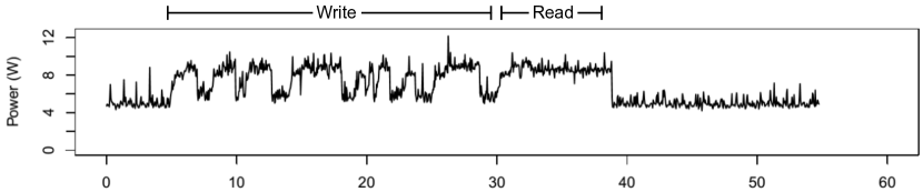
Figure 1: Energy outline of a program that writes a sequence of records into a file, and then reads them all.

Figure 2 illustrates which kind of information we can produce with JetsonLeap. Further examples shall be discussed in Section 4. The figure shows a chart that we have produced with JetsonLeap, for a program that performs different tasks: (i) initialize two $3,000\times 3,000$ matrices; (ii) multiply these matrices locally; (iii) send these matrices to a remote server; (iv) read back the product matrix, which was constructed remotely; (v) sum up the product matrix, to check if the result is correct; and (vi) repeat step (i). We repeat step (i) just for consistency: to ensure that multiple occurrences of the same event lead to very similar energy numbers. Notice that phases (ii) and (iii) have the same goal: to obtain the matrix that results from the multiplication of two other matrices. The difference between them is that in the former case the multiplication happens locally, and in the latter it happens remotely.

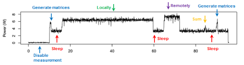
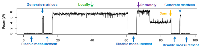
Figure 2: Example showing the energy consumed at different phases of a matrix multiplication program. (Top) Original chart, produced without our apparatus. (Bottom) Power chart produced with JetsonLeap.

We have forced the main program thread to sleep for 5 seconds in between each task. Using this approach, we have made the beginning and the end of each phase of the program visually noticeable. These marks, e.g., a 5 seconds low on the energy chart, lets us already draw one conclusion about this setup: it is better, from an energy perspective, to offload matrix multiplication, instead of performing it locally on the Tegra K1. However, this modus operandi, i.e., relying on visual identification clues to determine program phases, is far from being ideal. Its main shortcoming is the fact that it makes it virtually impossible to measure the energy consumed by program events of very small duration. We could, in principle, apply some border detection algorithm to identify changes in the energy pattern of the program. However, our own experience has shown that at a very low scale, border detection becomes extremely imprecise. One of the main contributions of this paper is to demonstrate that it is possible to mark – in an unambiguous way – a specific moment in the execution of a program to obtain its energy footprint.

The bottom part of Figure 2 shows the same chart, this time produced with the aid of our measurement apparatus. We have instrumented the program to deactivate energy measurement at the points where we call sleep. The visual separation between the different events of interest is more noticeable. However, more important than relying on visual clues, our instrumentation lets us determine precisely the points where energy numbers must be acquired. This type of acquisition is possible even when visual clues alone are not enough to distinguish the different events, as we shall explain in Section 3.

3 Measurement Infrastructure

The infrastructure of energy measurement that we provide consists of two parts: on the hardware side, we have an electric circuit that enables or disables the measurement of energy, according to program signals; on the software side, we have a library that gives developers the means to toggle energy acquisition; plus a program that reads the output of the power meter, and produces a report to the user. We have experimented with two different variations of the measurement circuit. All these variations use the same software package to acquire energy data. In this section we describe each one of these elements.

3.1 Circuit 1 – The Relay-Based Design

The first circuit that we use to gauge energy consumption uses a relay to enable or disable measurements. The relay is controlled by signals issued from the target program, in such a way that only regions of interest within the code are probed. Figure 3 shows this design. This apparatus consists of two sub-circuits; one of them enables and disables the power measurements using the relay. This relay connects the measurement probes across a shunt resistor. The resistance is 0.1$\Omega$ at 5W, and is connected in series with the 12V power supply input of the Jetson board. The other circuit is responsible for actuating the relay, and consists of a 4.7k$\Omega$ resistor at 0.25W, a BC547 transistor, and a flyback diode. The trigger of the relay is connected to a GPIO pin that in turn can be toggled by software.

Figure 3: Schematic view of the relay-based circuit that we use to measure energy in the Jetson board.

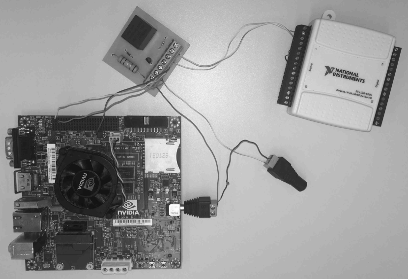
Figure 4: Circuit 1 – Relay-Based. (Top-Left) The circuit seen in Figure 3. (Bottom-Left) The Jetson board. (Top-Right) The NI 6009 data acquisition device

The measurement of the power spent by the circuit is controlled by the General Purpose I/O (GPIO) pin of the Jetson board. The GPIO port can be activated from any software that runs on the board. Each hardware defines GPIO ports in different ways; in our particular case, the Jetson has eight such ports, which we have highlighted in Figure 5 (top-right). Additionally, the 5V supply and the ground pins can be found in aforementioned figure. According to the Jetson’s programming sheet, these ports are located on pins 40, 43, 46, 49, 52, 55, 58, 50, J3A1 and J3A2 . Each port can be signalled independently.

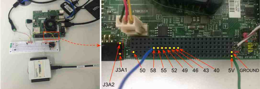
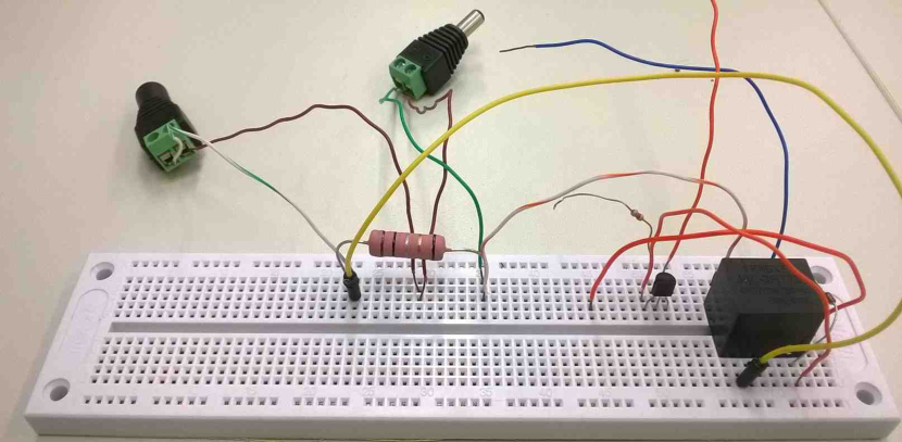
Figure 5: A picture of our apparatus. (Top-Left) The overall setup. (Top-Right) The ports on the Jetson board. (Bottom) Detailed view of the circuit. We use a protoboard to make the wiring more conspicuous.

Figure 3 shows that in the absence of positive signals on the GPIO port, the two cables of the power meter perform readings at the same logical region, which gives us a voltage of zero. Hence, energy will be zero as well. Upon activating a measurement –in face of a positive signal– the transistor lets energy flow to the relay, powering up its coil. In this way, the relay will connect each end of the resistor to each of the two power meter inputs, enabling the start of the power measurement. Using a data acquisition device (DAQ) to measure the value of $V_{s}$, the difference in voltage lets us probe the current at the shunt resistor. Using Equation 2, this gives us a way to know the current that flows into the Jetson board. Figure 4 shows how the circuit, the power meter and the Jetson board are connected.

3.2 Circuit 2 – The Trigger-Based Design

The circuit of Section 3.1 lets us measure fine-grained energy consumption events using a data acquisition device that has one probing channel. However, modern DAQs have more than one channel. As an example, the NI 6009 device that we use in this paper has 16 channels. In this case, we can replace the relay-based circuit with a much simpler design. This new design uses an extra probing channel to read signals directly from the GPIO port, triggering a measurement whenever the status of the port changes. Measurement commences once the power meter identifies a voltage drop in the shunt resistor between the power source and the Jetson board. Figure 6 shows a schematic view of the trigger-based design. This circuit contains only one electronic component: a 0.1$\Omega$ 5W resistor.

Figure 6: Schematic view of the circuit that uses two channels to measure energy in the Jetson board.

When compared to the relay-based design, this new approach has one important advantage: Using a second channel as a trigger has a much faster response time than using a relay to open or close the measurement circuit. Therefore, we can measure the energy consumption of events that take shorter time. On the other hand, there is a disadvantage: by using two channels, we split the precision of the power meter in half, because this device uses the same buffer to store data from all its channels. We have, however, not perceived any empirical difference between these two circuits in practice, because the energy behavior of the Jetson board does not show great variance in short periods of time.

3.3 Software

The software layer of our apparatus is made of two parts. First, we provide users with a simple library that lets them send signals to the GPIO port of the target device. Additionally, this library contains routines to record which ports are in use, and to log events already performed. Figure 7, in Section 4.1, shows a program that toggles the energy measurement circuit twice. To provide users with some amount of thread-safety, we let this toggling to be bound to identifiers. In this way, we can ensure that only one thread has the privileges to switch the state of the data-acquisition circuit.

The second part of our software layer is an interface with the data acquisition tool. We are currently using a National Instruments 6009 DAQ. During our first toils with this device, we have been using LabView  to read its output. LabView is a development environment provided by National Instruments itself; thus, it already comes with an interface with the DAQ. However, for the sake of flexibility, and in hopes of porting our system to different acquisition devices, we have coded a new interface ourselves. Our tool, called CMeasure, has been implemented in C++. It lets us (i) read data from the DAQ; (ii) integrate power, to obtain energy numbers; and (iii) produce energy reports. Concerning (ii), while in its idle state, our circuit still lets some noise pass to the DAQ, which oscillate between -0.001 and +0.001 watts. The expected value of this data’s integral is zero. Thus, by simply integrating the entire range of power values that we obtain through CMeasure, we expect to arrive at correct energy consumption with very high confidence.

4 Evaluation

In order to validate our energy measurement system, we have used it as the baseline platform to run different experiments. In this section, we discuss some of the results that we have obtained in the process. Section 4.1 starts our discussion by presenting data related to the precision of our approach. In particular, we investigate the minimum number of instructions whose execution we can detect using the two different circuits. At the end of the section, we show how our setup compares against more sophisticated equipment. Section 4.2 provides material that demonstrates the many possibilities that our platform opens up in the research community. These experiments compare the energy footprint of sequential, parallel (multi-core and GPU) and remote execution of programs. We emphasize that these experiments, per se, are not a contribution of this paper; rather, they illustrate the benefit of our framework. Nevertheless, these experiments are original: no previous work has performed them before on the Tegra board.

4.1 On the Accuracy and Precision of the JetsonLeap Apparatus

The goal of this section is to answer two research question:

Accuracy:

What is the minimum number of instructions whose energy budget we can measure with high confidence?

Precision:

How much information do we lose by using a sampling rate much inferior to the clock of the target device we measure?

Research Question 1 – Accuracy

In the context of this work, an event is a sequence of instructions processed during program execution. An ideal measurement device should estimate with high accuracy the power dissipated by events as small as one instruction. However, such precision, given the high frequency of modern hardware and the low sampling rate of data acquisition devices, is not possible. Our first research question asks us about the minimum event size that we can analyze with high confidence. To produce an answer to this question, we have used the program in Figure 7 (left) to find out the minimum number of ARM instructions whose energy footprint we can measure. This program runs a loop that only increments a counter for a given number of iterations. By varying the number of iterations, we can estimate the minimum quantity of instructions that gives us energy numbers that can be reproduced across multiple experiments. When compiled with gcc 4.2.1 -O1, the program in Figure 7 (left) yields a loop with three instructions: add, cmp, blt. Therefore, this program gives us a rough estimate of how many instructions we can measure: $T$ iterations yield $3T$ instructions.

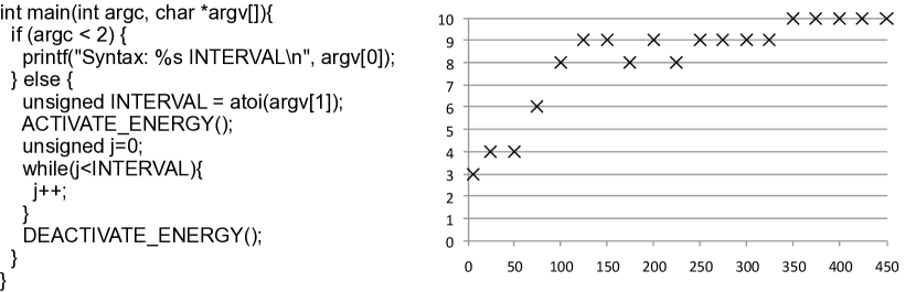
Figure 7: (Left) Program used to measure the precision of our apparatus. (Right) Chart relating the number of correct measurements with the value of INTERVAL in the program on the left, using the relay-based circuit. The Y axis gives us number of hits, out of 10 tries; the X axis gives us the value of INTERVAL (in thousands).

Figure 7 (right) gives us the result of this experiment for the relay-based circuit. For each value of INTERVAL, we have tried to obtain energy numbers 10 times. Whenever we obtain a measurement, we deem it a hit; otherwise, we call it a miss. We know precisely if we get a hit or a miss on each sample, because we can probe the state of the relay after we run the experiment. We started with INTERVAL equals to 5,000, and then moved on to 25,000. From there, we incremented INTERVAL by 25K, until reaching 450,000. For INTERVAL equal to 5,000, we have been able to switch the relay 3 out of 10 times. After we go past 325,000 iterations (975K instructions), we obtain 10 hits out of each 10 tries. These numbers are in accordance with the expected switching time of our relay, i.e., half a millisecond. Given that our ARM CPUs run at 2.3GHz during this experiment, we should expect no more than 2.3 million instructions per millisecond. To give the reader some perspective on the meaning of such numbers, we have counted the total number of instructions executed with $\mathtt{INTERVAL}=1$. We have removed the ACTIVATE_ENERGY and the DEACTIVATE_ENERGY macros from the source code. In this case, we have counted 7,237,290 instructions for the entire processor, which was executed on Linux Ubuntu 14.04. Out of this lot, 14,081 instructions execute in the main method alone; and the rest are kernel instructions. Most of these instruction are due to a loop before main that does a simple search on all library functions in order to find the right ones to link dynamically.

The trigger-based circuit shows higher precision. In this case, we obtain 10 hits out of 10 tries for $\mathtt{INTERVAL}=75,000$. And for $\mathtt{INTERVAL}=25,000$ we already obtain 8 hits out of 10 tries. In other words, we can change the state of the power measurement circuit, with high confidence, in intervals of $225,000$ instructions. This accuracy is more than four times higher than that observed when using the relay-based apparatus. We emphasize that the sampling rate of the relay-based circuit is higher: $40K/\mbox{sec}$, in contrast with $20K/\mbox{sec}$ when using the trigger-based design. As mentioned in Section 3.2, the lower sampling rate of the latter setting is due to the fact that we must reserve half the data acquisition channel to probe the GPIO port. Nevertheless, even this lower sampling rate is already higher than the average frequency used in related work. As an example, Stokke et al. read hardware performance counters at intervals of 100ms, in order to check the validity of their energy model for the Tegra K1 board [Stokke et al. (2015, 2016)].

Research Question 2 – Precision

The experiments that we perform in this paper use a relatively simple power meter: the NI 6009 Data Acquisition Device, which has a sampling rate of 40KHz. If we use the trigger-based design, this sampling rate falls to 20KHz, because we must reserve half the samples to probe the GPIO pin of the target board. Compared to the frequency of the Jetson board, 2.3GHz, this sampling rate is very small. The Nyquist Theorem [Nyquist (1928)] states that to avoid losing any information of an analog signal, we need to sample that signal with twice its frequency. If we assume that the power spent in processing instructions follows the frequency of the processor, then our infrastructure gives us a sampling rate much below Nyquist’s rate.

In order to verify how much information we are losing, we have performed the same measurements using a more accurate acquisition device. We do not have access to equipment that lets us sample energy consumption at the same rate as the frequency of the JetsonBoard, which is 2.3GHz at maximum clock. However, we do have access to a Keysight DSO-X 2022A Oscilloscope, whose sampling frequency is 200MHz. This frequency is 5,000x higher than the frequency of our NI 6009 power meter. In this section we benchmark the power meter against this oscilloscope. For this experiment, we used the relay-based circuit only for the power meter; for the oscilloscope, we estimated the points at which the trigger activated (upon program execution start) and deactivated (at execution stop). Through this arrangement, we could calculate the energy consumed by the Jetson board, in Joules. The integration of the oscilloscope’s instantaneous power measurements uses the approximation rule known as the “trapezoidal rule”.

Input size	Power meter		Oscilloscope
$1,000\times 1,000$	27.090	29.256	26.712	28.623
$1,500\times 1,500$	85.647	85.682	86.597	95.338
$2,000\times 2,000$	189.27	191.45	190.57	196.19
$2,500\times 2,500$	375.80	380.42	373.81	382.81
$3,000\times 3,000$	643.15	654.68	643.32	652.17

Table 1: Comparison of energy consumption (in Joules) with Cholesky algorithm execution on the Jetson board as measured by the power meter and oscilloscope. We show the lower and upper boundary for the results obtained by each device.

In this experiment we use two different devices to analyze the same Cholesky matrix factorization algorithm. The tests were exclusively executed on one of the Jetson’s CPUs, with squared matrices of size $1,000$, $1,500$, $2,000$, $2,500$ and $3,000$ cells. Table 1 shows the results of the experimental comparisons. Results are very similar and within the margins of error specified in Table 2. For each chosen input size, we have, thus, produced five different energy samples in order to determine the margin of error. Table 2 shows the five samples produced using the oscilloscope. We have interposed a waiting time between samples to avoid overheating the processor. The perceived variation between samples when using the power meter, was less than 1%, given the same input size. This variation, when using the oscilloscope, was less than 2%.

Cholesky	Test1	Test2	Test3	Test4	Test5	Mean	ME
1000	26.712	29.644	27.567	28.623	27.453	28.000	1.421
1500	93.514	91.412	92.680	95.338	86.597	91.908	4.090
2000	196.19	192.67	190.57	193.42	192.79	193.13	2.507
2500	374.79	382.81	381.47	382.68	373.81	379.11	5.509
3000	643.40	652.17	645.31	643.32	649.38	646.71	4.860

Table 2: Energy consumption (in Joules) with the Cholesky algorithm execution on the Jetson board as measured by the oscilloscope. Five measurements were made for each Cholesky matrix size. The Margin of Error (ME) was calculated based on all data from each of the Cholesky sizes, using a t-score based on a 95% confidence level and degrees of freedom of 4.

.

4.2 Applications of JetsonLeap

One of the contributions of this paper is to show that we can use JetsonLeap to perform several kinds of experiments. In the rest of this section we go over some of these experiments.

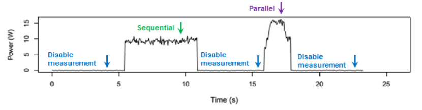
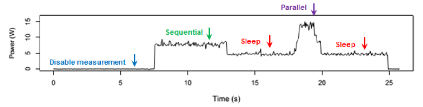
Figure 8: Energy outline of a program that runs different versions of mergesort. (Top) Chart produced with our apparatus. (Bottom) Chart produced without energy toggling. We use a 5-seconds sleep time to separate the execution of the different implementations.

Parallel vs Sequential CPU code

What is more energy efficient: to run some computation sequentially, in a single core, or to split it into multiple cores that execute in parallel? Different applications are likely to show different behaviors under these two distinct circumstances. JetsonLeap lets us probe such behavior for a particular application. To demonstrate this possibility, we have used it to analyze the energetic footprint of two different implementations of merge-sort: sequential and parallel. Both applications used in this section sort the same array of integers. They have been compiled with gcc 4.2.1, at the -O3. The parallel implementation of merge-sort uses Posix Threads.

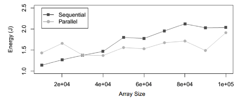
Figure 9: Energy consumed by different versions of a mergesort routine.

Figure 8 (Top) shows a power chart for the two different implementations of merge-sort when sorting arrays of 1,000,000 integers. The sequential implementation is slower: it takes about 5.2 seconds to sort the input array. Its parallel equivalent takes about 2.4 seconds to perform the same task. However, the sequential version runs on less power: about 9W. The parallel implementation, on the other hand, peaks at 15W. Yet, it does not use this power at every point of its execution: as less and less parallelism becomes available, it tends to use less threads. This observation explains the spiky outline of the chart that JetsonLeap produces for the parallel merge-sort. For this specific input, an array of one million cells, the faster runtime pays off: our parallel merge-sort uses approximately 65% of the energy spent by the sequential version.

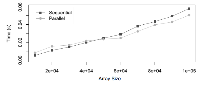
Figure 10: Runtime for different versions of a mergesort routine.

This experiment raises another interesting question: is the parallel implementation of merge-sort always more energy efficient than the sequential code? In search of answers for this question, we have fed both implementations with arrays of different sizes. For small inputs, the sequential algorithm runs faster, and tends to be more energy efficient. Figure 9 shows energy consumption probed for inputs of different sizes. For this specific experiment, we have observed that up to arrays of 30,000 cells, the sequential implementation uses less energy. Past this size, the parallel version fares consistently better. We run each sample only twice; hence, these constants may suffer small variations in new rounds of this very experiment.

Figure 10 shows the runtime observed in the comparison between the different sorting approaches with small inputs. There is a very strong correlation between runtime and energy: the faster implementation tends to be the more energetically efficient. However, in this experiment we have observed a small window, extending from arrays of 30,000 to 40,000 cells, when the faster parallel implementation spends more energy than the slower sequential algorithm. This behavior has been reproduced consistently in further repetitions of the same experiment.

A Brief Evaluation of Code Offloading Techniques

Code offloading consists of sending to an external host computation that the local processor deems worthy of executing remotely. Modern heterogeneous architectures furnish developers with a plethora of strategies to offload code. As an example, the TK1 board gives us the following alternatives to run computation: the quad-core CPUs, the low-power ARM core and the GPU. Additionally, we can offload code to a remote server, trading computation for bandwidth. To explore these different resources, we have used them to execute two programs: matrix multiplication and matrix addition. Even though conceptually very simple, these two programs present us with diametrically opposite behaviors, as we show empirically.

Figure 11: (Top) Energetic behaviour of matrix multiplication running on different processors. (Bottom) Energetic behaviour of matrix addition running on different processors.

Figure 11 summarizes these experiments. The most power-efficient configuration for matrix multiplication consists of running it on the GPU, or on the remote server. To give the reader an idea about such tradeoffs, we spend 274.0J to multiply a $2500\times 2500$ matrix on the GPU; 737.8J to perform the same operation on the ARM CPU, 4,639.6J if using the low-power core, and 310.1J to offload the computation to a remote server. Figure 2 shows the energy outline to perform the multiplication locally, on the standard CPU, and remotely. In the latter scenario, all the energy spending is due to network communication, plus idle waiting. As Figure 2 shows, the instantaneous power consumed in networking is slightly higher than the power spent by CPU intensive computations; however, the faster runtime of the server is enough to pay off for the energy wasted with data movement.

Once we consider matrix addition we are giving a diametrically opposed picture: we spend 0.91J to perform the addition on the low-power core, and 7.4J to run the same operation on the standard CPU. Once we go to the graphics processor, this number increases tenfold: we spent 72.9J to run matrix addition on the GPU. Finally, if we offload the computation to a remote server, we pay a fee of 195.5J.

This remarkable difference between the two algorithms, matrix multiplication and matrix addition, is a consequence of their asymptotic complexities: matrix addition involves $O(N^{2})$ floating-point operations on $O(N^{2})$ elements of a $N\times N$ matrix. Therefore, its computation over data ratio is $O(1)$. Thus, the time to transfer data between devices already shadows any gains from parallelism and offloading. On the other hand, when it comes to the multiplication of matrices, sending the data to a server is beneficial after a certain threshold. Matrix multiplication has higher asymptotic complexity than matrix addition, e.g., the former performs $O(N^{3})$ floating-point operations. Yet, the amount of data that both algorithms manipulate is still the same: $O(N^{2})$. Thus, in the case of matrix multiplication we have a linear ratio of computation over data, a fact that makes offloading much more advantageous.

Static Scheduling of Code on Heterogeneous Devices – Manual Annotations

JetsonLeap allows us to compare the energy consumption of a program running on the CPU, versus the energy consumption of similar code running on the GPU. To demonstrate this possibility, we use a benchmark suite made of six programs, which we took from Etino, a tool that analyzes the asymptotic complexity of algorithms [Demontiê et al. (2015)]. These programs are mostly related to linear algebra: Cholesky and LU decomposition, matrix multiplication and matrix sum. The other two programs are Collinear List, which finds collinear points among a set of samples, and Str. Matching, which finds patterns within strings. All these are written in standard C, without any adaptations for a Graphics Processing Unit (GPU). To compile these programs to the Tegra’s GPU, we have used DawnCC [Mendonca et al. (2016)] to annotate them with OpenACC directives. Each benchmark has only one core loop, which implements the bulk of the processing. OpenACC is an annotation system that lets developers indicate to the compiler which program parts are embarrassingly parallel, and can run on the graphics card. We have used accULL [Reyes et al. (2012)] to produce GPU binaries out of annotated programs. The code that runs on the CPU has been produced with gcc 4.2.1, at the -O3 optimization level. Therefore, in this experiment we are comparing, in essence, the product of different compilers, – targeting different processors – when given the same source code.

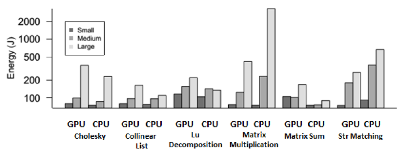
Figure 12: Energy consumed by different programs, running either on the CPU, or on the GPU.

Figure 12 shows the energy consumed by each benchmark, and Figure 13 shows the time that each program takes to execute. For each benchmark, we show results for the three different input sizes that are available in the original distribution of Etino. All the results that we produce for the GPU include the time (and energy) to copy data between host (CPU) and device (GPU) processors. We have observed that the GPU code runs faster than its CPU counterpart; however, oftentimes this extra speed is not enough to pay for the cost of moving data. Thus, for many benchmarks, the Tegra GPU yields worst results than the ARM CPU.

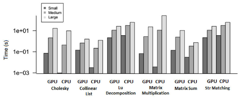
Figure 13: Runtime for different programs, running either on the CPU, or on the GPU.

There exists a strong correlation between runtime and energy consumption; however, there are situations in which the GPU is faster, but spends more energy. Such fact happens twice, in Lu Decomposition and String Matching. This result corroborates some of the conclusions drawn by Pinto et al. [Pinto et al. (2014)], who have shown that after a certain threshold, an excessive number of threads may be less energy efficient, even for data-parallel applications. Notice that they have gotten their results comparing code running on a multi-core CPU with a different number of cores enabled each time. Figure 14 supports our observation. It shows a program that performs matrix summation, first on the GPU, and then on the CPU. The difference in power consumption makes it easy to tell each phase apart. During the whole execution of the GPU, its power dissipation is higher than the CPU’s. We believe that these results are particularly interesting, because they show very clearly that in some scenarios, runtime is not always proportional to energy consumption.

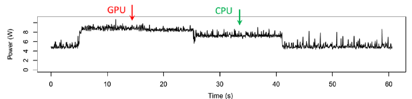
Figure 14: A chart that illustrates the difference between power consumption by a program running on the GPU and on the CPU.

Static Scheduling of Code on Heterogeneous Devices – Automatic Annotations

In the previous discussion, we have manually annotated a series of simple benchmarks with OpenACC directives, and have compared them when running on the CPU, or on the GPU. This time we repeat this experiment, but now using an automatic parallelizer, dawn-cc [Mendonca et al. (2016)]. This tool is available through an on-line server which reads C sources, and produces C sources annotated with either OpenACC or OpenMP directives. The tool’s distribution packs a benchmark suite, which we shall use in this experiment. These benchmarks are publicly available.

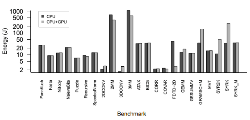
Figure 15: Energy consumed by different programs, running either on the CPU, or on the CPU and GPU.

For each benchmark, we run its original version on the TK1’s CPU, and then feed it to dawn-cc, to obtain an equivalent program annotated with OpenACC directives. Again, we use AccULL to compile the annotated program. Contrary to the benchmark suite used in Figures 12 and 13, this new set of programs contain several loops. The automatic annotator uses a collection of heuristics to determine the parts of the program that must be sent to the GPU. Annotations have been produced for all the benchmarks, except Fannkuch, Fasta, NBody, NsieveBits and SpectralNorm. Nevertheless, we show the runtime and energy consumption of these benchmarks, so that our results can be compared against the original work on dawn-cc.

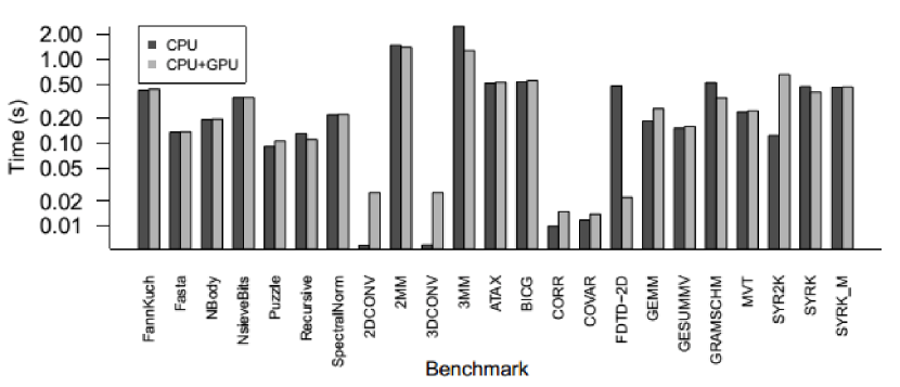
Figure 16: Runtime for different programs, running either on the CPU, or on the CPU and GPU.

Figures 15 and 16 summarize the results of this experiment. As observed with manual annotations, there is a correlation between runtime and energy consumption. Nevertheless, again we observe situations in which the GPU runs faster, but spends more energy. For instance, GRAMSCHM, an implementation of the Gram–Schmidt process, we have that the GPU version is 10% faster than the CPU’s, but consumes 30% more energy. We remind the reader that these numbers take into consideration the time and energy necessary to copy data between CPU and GPU.

5 Related Work

Much has been done, recently, to enable the reliable acquisition of power data from computing machinery. In this section we go over a few related work, focusing on the unique characteristics of our JetsonLeap. Before we commence our discussion, we emphasize a point: a lot of related literature uses energy models to derive metrics [Dunkels et al. (2007); Steinke et al. (2002); Stokke et al. (2016)]. Even though we do not contest the validity of these results, we are interested in direct energy probing. Thus, models, i.e., indirect estimation, are not part of this survey. Nevertheless, we believe that an infrastructure such as JetsonLeap can be used to calibrate new analytical models.

The most direct inspiration of this work has been AtomLeap [Peterson et al. (2011)]. Like JetsonLEAP, AtomLeap is also a system to measure energy in a System-on-a-Chip device. However, Singh et al. have chosen to use the Intel Atom board as their platform of choice. Furthermore, they do not use a circuit, like we do, to toggle energy measurement. Instead, they synchronize the Atom’s clock with a global watch used by the energy measurement infrastructure. By logging the time when particular events take place during the execution of a program, they are able to estimate the amount of energy consumed during a period of interest. They have not reported on the accuracy of this technique, so we cannot compare it against our approach. We believe that the Nvidia setup gives us the opportunity to log more interesting results, given that this hardware provides more variety of processors. In addition to AtomLeap, our work is also related to ARDUPOWER [Dolz et al. (2015)], which is a low-power Wattmeter for HPC applications. The key difference to our work is measurement granularity, which constrains the ARDUPOWER to monitor only power events in the range of seconds.

There is previous work that attempt to recognize programming events by means of border detection algorithms. This is, for instance, the approach of Silva et al. [Silva et al. (2014)], or Nazare et al [Nazaré et al. (2014)]. The idea is simple: if we assume that the hardware consumes more energy when it runs a program, then we can expect an isolated, flat-topped hill on its energy skyline. Thus, the amount of energy in this clearly visible area corresponds to the amount of energy spent by the program. Such a methodology works to measure the energy spent by a program that runs for a relatively long time; however, it cannot be applied to probe short programming events, like we do in this paper. The reasons for this limitation are two-fold. First, internal program events might not produce visual clues that denounce their existence. Second, our own experience reveals that border detection requires a considerable number of sampling points to work reliably. This requirement would greatly reduce its precision when necessary to detect fast events.

A final technique that is worth mentioning relies on hardware counters, such as Intel’s RAPL (Running average power limit). Different hardware provides different kinds of performance counters, which might log runtime, memory traffic or energy. RAPL registers can be used to keep track of very fast programming events, as demonstrated by Hähnel et al [Hähnel et al. (2012)]. Zheng et al [Zheng et al. (2016)] proposes a learning algorithm that uses hardware counter information to estimate power consumption of different platforms. Along similar lines, Stokke et al. [Stokke et al. (2015, 2016)] have built what is possibly the most precise energy model nowadays available for the TK1 board using counters. Nevertheless, only a limited range of computing machinery provides such tools. Thus, techniques such as ours are still essential for simpler hardware. Additionally, direct approaches tend to earn more trust from the research community [Weaver et al. (2012)].

Contrary to AtomLEAP and similar approaches [Ge et al. (2010); McIntire et al. (2012)], our infrastructure does not allow us to measure the power dissipation of separate components within the hardware, such as RAM, disks and processors. This limitation is a consequence of the heavy integration that exists between the many components that form the Nvidia TK1 board. Implementing energy measurement in such environment, at component level is outside the scope of this work. Nevertheless, a comparison with the work of Ge et al. [Ge et al. (2010)] is illustrative. They use two data acquisition devices to probe different parts of the hardware simultaneously. Synchronisation is performed through a client-server architecture, via time-stamps. Although the authors have not reported the length of programming events that they can measure, we believe that our approach enables finer measurements, as we do not experiment network delays. Besides, our infrastructure is cheaper: the fact that we control the acquisition circuitry from within the target program lets us use a simpler power meter – even a probe with a single channel works in our case.

6 Conclusion

This paper has presented JetsonLeap, an apparatus to measure energy consumption in programs running on the Nvidia Tegra board. JetsonLeap offers a number of advantages to developers and compiler writers, when compared to similar alternatives. First, it allows acquiring energy data from very brief programming events: our experiments reveal a precision of about 225,000 instructions, given a clock of 2.3GHz. Such granularity enables the measurement of power-aware compiler optimizations, for instance. Second, our infrastructure is cheap: the entire framework can be constructed with less than $ 500.00, including power meter and processor. Finally, it is general: we have built it on top of a specific platform, the Nvidia Jetson TK1 board. However, the only essential feature that we require on the target hardware is the existence of a general purpose input-output port. Such port is part of the design of several different kinds of System-on-a-Chip devices, including open-source hardware, such as the many variations of the Arduino single-board microcontroller.

Reproducibility

Further instructions about how to reproduce our apparatus are available at this project’s webpage: http://cuda.dcc.ufmg.br/jetson/. This site contains manuals to build the two different circuits that we use, and to integrate them with the software stack that we have implemented. We also provide an implementation of CMeasure, our interface with the data acquisition device used in this work.

Acknowledgement

This work have been partially funded by the Brazilian Ministry of Science, Technology, Innovation and Communication through the National Research Council (CNPq), by the Brazilian Ministry of Education, and by EUBra-BIGSEA (EC Cooperation Programme H2020 690116) and Brazilian MCTI/RNP (GA-0000000650/04).

References

References

- Beloglazov et al. (2012) Beloglazov, A., Abawajy, J., Buyya, R., 2012. Energy-aware resource allocation heuristics for efficient management of data centers for cloud computing. Future Gener. Comput. Syst. 28 (5), 755–768.
- Bessa et al. (2016) Bessa, T., Quintão, P., Frank, M., Pereira, F. M. Q., 2016. Jetsonleap: A framework to measure energy-aware code optimizations in embedded and heterogeneous systems. In: SBLP. Springer, pp. 16–30.
- Demontiê et al. (2015) Demontiê, F., Cezar, J., da Silva Bigonha, M. A., Campos, F., Pereira, F. M. Q., 2015. Automatic inference of loop complexity through polynomial interpolation. In: SBLP. Springer, pp. 1–15.
- Dolz et al. (2015) Dolz, M. F., Heidari, M. R., Kuhn, M., Ludwig, T., Fabregat, G., Dec 2015. Ardupower: A low-cost wattmeter to improve energy efficiency of hpc applications. In: Green Computing Conference and Sustainable Computing Conference (IGSC), 2015 Sixth International. pp. 1–8.
- Dunkels et al. (2007) Dunkels, A., Osterlind, F., Tsiftes, N., He, Z., 2007. Software-based on-line energy estimation for sensor nodes. In: EmNets. ACM, pp. 28–32.
- Ge et al. (2010) Ge, R., Feng, X., Song, S., Chang, H.-C., Li, D., Cameron, K. W., 2010. Powerpack: Energy profiling and analysis of high-performance systems and applications. IEEE Trans. Parallel Distrib. Syst. 21 (5), 658–671.
- Hähnel et al. (2012) Hähnel, M., Döbel, B., Völp, M., Härtig, H., 2012. Measuring energy consumption for short code paths using rapl. SIGMETRICS Perform. Eval. Rev. 40 (3), 13–17.
- McIntire et al. (2006) McIntire, D., Ho, K., Yip, B., Singh, A., Wu, W., Kaiser, W. J., 2006. The low power energy aware processing (leap)embedded networked sensor system. In: IPSN. ACM, pp. 449–457.
- McIntire et al. (2012) McIntire, D., Stathopoulos, T., Reddy, S., Schmidt, T., Kaiser, W. J., 2012. Energy-efficient sensing with the low power, energy aware processing (LEAP) architecture. ACM Trans. Embedded Comput. Syst. 11 (2), 27.
- Mendonca et al. (2016) Mendonca, G. S. D., Guimaraes, B. C. F., Alves, P. R. O., Pereira, M. M., Araujo, G., Pereira, F. M. Q., 2016. Automatic insertion of copy annotation in data-parallel programs. In: SBAC-PAD. IEEE, pp. 1–8.
- Nazaré et al. (2014) Nazaré, H., Maffra, I., Santos, W., Barbosa, L., Gonnord, L., Pereira, F. M. Q., 2014. Validation of memory accesses through symbolic analyses. In: In OOPSLA. ACM, pp. 791–809.
- Neto (2016) Neto, J. L. D., 2016. ULOOF: User-Level Online Offloading Framework. Master’s thesis, UFMG.
- Neto et al. (2016) Neto, J. L. D., Macedo, D. F., Nogueira, J. M. S., 2016. A location aware decision engine to offload mobile computation to the cloud. In: NOMS. pp. 831–838.
- Nyquist (1928) Nyquist, H., 1928. Certain topics in telegraph transmission theory. Transactions of the AIEE 47, 617–644.
- Peterson et al. (2011) Peterson, P. A. H., Singh, D., Kaiser, W. J., Reiher, P. L., 2011. Investigating energy and security trade-offs in the classroom with the Atom LEAP testbed. In: CSET. USENIX, pp. 1–11.
- Pinto et al. (2014) Pinto, G., Castor, F., Liu, Y. D., 2014. Understanding energy behaviors of thread management constructs. In: OOPSLA. ACM, pp. 345–360.
- Reyes et al. (2012) Reyes, R., López-Rodríguez, I., Fumero, J. J., de Sande, F., 2012. accull: An openacc implementation with cuda and opencl support. In: Euro-Par. Springer, pp. 871–882.
- Saputra et al. (2002) Saputra, H., Kandemir, M., Vijaykrishnan, N., Irwin, M. J., Hu, J. S., Hsu, C.-H., Kremer, U., 2002. Energy-conscious compilation based on voltage scaling. In: SCOPES. ACM, pp. 2–11.
- Sartori and Kumar (2012) Sartori, J., Kumar, R., 2012. Compiling for energy efficiency on timing speculative processors. In: DAC. ACM, pp. 1301–1308.
- Silva et al. (2014) Silva, B. L. B., Tavares, E. A. G., Maciel, P. R. M., e Silva Nogueira, B. C., Oliveira, J., Damaso, A. V. L., Rosa, N. S., 2014. AMALGHMA -an environment for measuring execution time and energy consumption in embedded systems. In: SMC. IEEE, pp. 3364–3369.
- Steinke et al. (2002) Steinke, S., Wehmeyer, L., Lee, B., Marwedel, P., 2002. Assigning program and data objects to scratchpad for energy reduction. In: DATE. IEEE, pp. 409–415.
- Stokke et al. (2015) Stokke, K. R., Stensland, H. K., Griwodz, C., Halvorsen, P., 2015. Energy efficient video encoding using the tegra k1 mobile processor. In: MMSys. IEEE, pp. 81–84.
- Stokke et al. (2016) Stokke, K. R., Stensland, H. K., Halvorsen, P., Griwodz, C., 2016. High-precision power modelling of the tegra K1 variable SMP processor architecture. In: MCSoC. IEEE, pp. 1–8.
- Valluri and John (2001) Valluri, M., John, L. K., 2001. Interaction between Compilers and Computer Architectures. Springer, Ch. Is Compiling for Performance — Compiling for Power?, pp. 101–115.
- Vetro et al. (2013) Vetro, A., Ardito, L., Procaccianti, G., Morisio, M., 2013. Definition, implementation and validation of energy code smells: an exploratory study on an embedded system. In: ENERGY. pp. 34–39.
- Weaver et al. (2012) Weaver, V. M., Johnson, M., Kasichayanula, K., Ralph, J., Luszczek, P., Terpstra, D., Moore, S., 2012. Measuring energy and power with papi. In: ICPPW. IEEE, pp. 262–268.
- Wienke et al. (2012) Wienke, S., Springer, P., Terboven, C., an Mey, D., 2012. OpenACC: First experiences with real-world applications. In: Euro-Par. Springer, pp. 859–870.
- Yuki and Rajopadhye (2013) Yuki, T., Rajopadhye, S. V., 2013. Folklore confirmed: Compiling for speed = compiling for energy. In: LCPC. pp. 169–184.
- Zheng et al. (2016) Zheng, X., John, L. K., Gerstlauer, A., 2016. Accurate phase-level cross-platform power and performance estimation. In: DAC. ACM, pp. 4:1–4:6.