Bianchi I Cosmology and Scalar Vector Tensor Brans Dicke Gravity

Abstract

We consider Brans Dicke scalar vector tensor gravity to study an inflationary scenario of the accelerating expansion of the universe for which the anisotropy property occurs. We study both primordial inflation and late inflationary period of the universe. To do so we, use Bianchi I line element where spatial part has cylindrical symmetry along $x$ direction in the local Cartesian coordinates. To seek stabilization of our obtained metric solution, we apply dynamical system approach to obtain critical manifolds in phase space and determine which of them confirms the inflation with stable nature in presence of the anisotropy property of spacetime. We solve dynamical equations for different directions of the timelike dynamical vector field. We obtain several critical manifolds whose nature of stable (sink) or quasi stable (saddle) are dependent on the direction of the used vector field. At last, we should point that observational constraint on the Brans Dicke parameter $\omega>40000$ which satisfied by the well known Brans Dicke scalar tensor gravity is not valid for our modified scalar vector Brans Dicke gravity because of presence of timelike dynamical vector field.

1 Introduction

The $\Lambda CDM$ model which is confirmed by the standard cosmology has a great success in explaining the observations of the cosmic microwave background radiation (CMBR) temperature anisotropy, as well as the galaxies distribution and whose motion [1, 2, 3, 4]. This model which is based on the validity of the cosmological principle (the spatial homogeneity and spatial isotropy) and the Einstein‘s general theory of relativity explain most large-scale observations with unprecedented accuracy. However, several directional anomalies have been reported in various large-scale observations. In short these anomalies are called as follows: the polarization distribution of the quasars [5], the velocity flow [6, 7, 8], the handedness of the spiral galaxies [9, 10, 11], the anisotropy of the cosmic acceleration [12, 13, 14, 15, 16, 17], the anisotropic evolution of fine-structure constant [18, 19, 20] and asymmetry of the CMBR parity [21, 22, 23, 24, 25]. In fact, origin of these anomalies do not still understood and so they treat as puzzles. There are two different proposals to understand these problems as follows: The first perhaps is they are originated from cosmological effects which should be described via alternative gravity theories instead of the Einstein‘s general theory of relativity. Other possibility which arises these directional anomalies can be systematic errors or contaminations of measuring instruments and etc., which should be excluded from the future data analysis. In the latter case, one usually accept validity of the standard cosmological $\Lambda CDM$ model while in the former proposal one use an alternative gravity model instead of the Einstein‘s general theory of relativity. Zhao and Santos, did provided full review about these proposals [26] where the directional anomalies predict a preferred axis called as ‘Axis of Evil‘ in large scale of the Universe. In short, they compared the preferred directions in large-scale observations and the CMBR kinematic dipole and found a strong alignment between them. In fact, CMB radiation dipole is caused by motion of the solar system in the universe which is a non-cosmological effect. For review on data results of WMAP (Wilkinson-microwave anisotropy probe) and the Planck satellite, one can see references [27, 28, 29, 30, 31, 32, 33, 34, 35, 36, 37, 38, 39]. However, some alternative cosmological models are provided to satisfy these anomalies where the cosmological principle (spatial homogeneity and spatial isotropy in large scales structure) should be violated. In general, anisotropic curved spacetimes should be supported by anisotropic stress energy tensor of matter fields which are not present in the standard FLRW cosmology [40, 41]. For anisotropic vector field models, one can see [42, 43] and for anisotropic cosmological constant with dark energy [44, 45, 46, 47, 48, 49, 50, 51, 52, 53, 54, 55, 56, 57]. See also [53, 54, 55] which describe homogeneous but anisotropic Kantowski-Sachs cosmological model. To describe the above mentioned anomalies, it is shown that the anisotropic Bianchi cosmological models are applicable by anisotropic cosmological constant [56, 57] and by dark energy [53, 54, 55, 56, 57, 58]. From the point of view of elementary particle physics, several candidates have been identified for the particle carrying dark energy or dark matter and introduced to the world of science. The multiplicity of these candidates makes unknown origin of dark sector of matter/energy. Because of this some scientists use other gravitational models by regarding principle of general covariance (laws of Physics are the same for all observers and, therefore, must be written in terms of geometric objects), in which timelike dynamical vector fields coupled with the geometry produce gravitational corrections instead of the effects of unknown dark sector. Such models are called Einstein-Aether gravity usually in which the used timelike dynamical vector fields can be interpreted as four vector velocity of preferred reference frames. In fact these dynamical timelike vector fields break rotational symmetry of spacetime because there is interaction between the vector field and the geometry which will have bimetric(see introduction section of reference [59] for more discussion).

As a generalization of Einstein-Aether gravity, we consider a scalar-vector-tensor gravity model [59, 60] which is made from generalization of the well known Jordan-Brans-Dicke scalar tensor gravity [61] by transforming the background metric such that $g_{\mu\nu}\to g_{\mu\nu}+2N_{\mu}N_{\nu}$ in which $N_{\mu}$ is dynamical timelike four vector field. In the latter model, there is a non-minimal interaction between the Brans Dicke scalar field and the timelike vector field and in the present work we will see that it is possible to have the vector field whose spatial part does not vanish with the evolution (unless it has always been zero) pointing towards a direction which is different to the one of the rotational symmetry. This is what we call ”preferred reference frame effects”. Several applications of the model [59, 60] are studied for classical and quantum approach of FLRW cosmology [62, 63, 64, 65, 66] previously. In the present work, we investigate affects of a timelike dynamical massless vector field $N_{\mu}$ interacting with the Brans Dicke scalar field, on anisotropy property of a Bianchi I cosmology. To solve the gravitational field equations we use dynamical system approach and we obtain some critical manifolds with stable or quasi stable nature in phase space for each of four directions of the vector field which asymptotically are reduced to the de Sitter epoch with anisotropy trajectories. However, we determined stability nature of the obtained critical manifolds which are dependent to spatial directions of the used the dynamical vector field. Organization of the paper is as follows.

In section 2, we introduce the scalar vector tensor Brans Dicke gravity model [59, 60] briefly. In section 3, we use the Bianchi I background metric to obtain exact form of dynamical field equations. We solve gravitational equations by using dynamical systems approach. We determine critical manifolds in phase space of dynamical equations in presence of small perturbations of anisotropy property of the spacetime for each of four directions of the timelike dynamical vector field. Section 4 assign to concluding remark and outlook of the work.

2 The Model

Let us start with the following scalar-vector-tensor-gravity action [59, 60]

$$I_{total}=I_{BD}+I_{N},$$ (1)

where

$$I_{BD}=\frac{1}{16\pi}\int dx^{4}\sqrt{g}\left\{\phi R-\frac{\omega}{\phi}g^{\mu\nu}\nabla_{\mu}\phi\nabla_{\nu}\phi\right\},$$ (2)

is the well known Brans Dicke scalar tensor action [61], and with definitions

$$F_{\mu\nu}=2(\nabla_{\mu}N_{\nu}-\nabla_{\nu}N_{\mu}),~{}~{}~{}~{}~{}~{}~{}\Omega_{\mu\nu}=2(\nabla_{\mu}N_{\nu}+\nabla_{\nu}N_{\mu}),$$ (3)

the action functional

$$I_{N}= \frac{1}{16\pi}\int dx^{4}\sqrt{g}\{\zeta(x^{\nu})(g^{\mu\nu}N_{\mu}N_{\nu}+1)+2\phi F_{\mu\nu}F^{\mu\nu}-U(\phi,N_{\mu})$$

$$-\phi N_{\mu}N^{\nu}(2F^{\mu\lambda}\Omega_{\nu\lambda}+F^{\mu\lambda}F_{\nu\lambda}+\Omega^{\mu\lambda}\Omega_{\nu\lambda}-2R^{\mu}_{\nu}+\frac{2\omega}{\phi^{2}}\nabla^{\mu}\phi\nabla_{\nu}\phi)\},$$ (4)

describes dynamics of a unit timelike four vector field $N_{\mu}$ which can be considered as four velocity of a dynamical preferred reference frame which is couple non minimally with the Brans Dicke scalar tensor gravity. In fact, we assume that $N_{\mu}$ satisfies

$$g_{\mu\nu}N^{\mu}N^{\nu}=-1,$$ (5)

and such a model is named as Einstein-Aether gravity models in the literature. In fact, the general covariance principle leads us to consider $N_{\mu}$ as a dynamical vector field. $\zeta(x^{\mu})$ is undetermined Lagrange multiplier and $U(\phi,N_{\mu})$ is interacting potential between scalar and vector fields. Without the additional terms $\zeta$ and $U$ the action functional (2) is generated from (2) by regarding the metric transformation $g_{\mu\nu}\to g_{\mu\nu}+2N_{\mu}N_{\nu}$. One can check references [59, 60] to see detail of calculations. The action functional (2) shows that the vector field $N_{\mu}$ is coupled as non-minimally with the Brans Dicke scalar field $\phi.$ The action functional (1) is written in units $c=\hbar=1$ with Lorentzian signature (-,+,+,+). The undetermined Lagrange multiplier $\zeta(x^{\nu})$ controls $N_{\mu}$ to be unit timelike vector field. According to the Mach‘s principle [61] the Brans Dicke scalar field $\phi$ describes inverse of Newton‘s gravitational coupling parameter as $\phi(x)\sim\frac{1}{G(x)}$ and its dimension is $(lenght)^{-2}$ in units $c=\hbar=1$. Authors in reference [61] showed that to have an inflationary model for FRW metric the Brans Dicke scalar field should be a raising function versus the cosmic comoving time and this theory reduces to general theory of relativity at $\omega\to\infty.$ While our mathematical calculations show that the constraint on the $\omega$ parameter in Brans Dicke gravity does not valid in our modified scalar vector model. This is because our stable solutions are happened at small values of $\omega$ parameter. But fortunately, these solutions have stable nature in phase space with a raising function for the Brans Dicke field solution in both inflationary epochs and for all different directions of the vector field. With this view, it seems there is non minimal interaction between the timelike vector field and the Brans Dicke scalar field can resolve the inconsistency problem (why constraint on large values of the $\omega$ parameter does not consistent with our modified gravity theory). $g$ is absolute value of determinant of the metric field $g_{\mu\nu}$. Present limits of dimensionless Brans Dicke $\omega$ parameter based on time-delay experiments [67, 68, 69, 70] requires $\omega\geq 4\times 10^{4}$, but we will see this constraint can be violated in the alternative gravity model (1). Recently, authors of the work [72] investigated on constraining an exact Brans Dicke gravity with recent observations and obtained $\omega>1627.$

By varying (1) with respect to $\zeta(x^{\nu})$ we obtain (5) and by varying (1) with respect to the fields $\phi,$ $N^{\mu}$ and $g^{\mu\nu}$, we obtain corresponding dynamical equations respectively as follows

$$\frac{2\omega\Box\phi}{\phi}-\frac{\omega g^{\mu\nu}\partial_{\mu}\phi\partial_{\nu}\phi}{\phi^{2}}-\frac{4\omega N^{\mu}N^{\nu}\partial_{\mu}(\sqrt{g}\partial_{\nu}\phi)}{\phi\sqrt{g}}-\frac{\partial U(\phi,N_{\mu},)}{\partial\phi}$$

$$-\frac{4\omega\partial_{\mu}(N^{\mu}N^{\nu})\partial_{\nu}\phi}{\phi}-\frac{4\omega\Gamma^{\mu}_{\mu\alpha}N^{\alpha}N^{\nu}\partial_{\nu}\phi}{\phi}-\frac{4\omega\Gamma^{\nu}_{\mu\lambda}N^{\mu}N^{\lambda}\partial_{\nu}\phi}{\phi}+\frac{2\omega N^{\mu}N^{\nu}\partial_{\mu}\phi\partial_{\nu}\phi}{\phi^{2}}$$

$$+R-2N^{\mu}N^{\nu}R_{\mu\nu}+2F_{\mu\nu}F^{\mu\nu}-N_{\mu}N^{\nu}\{2F^{\mu\lambda}\Omega_{\nu\lambda}+F^{\mu\lambda}F_{\nu\lambda}+\Omega^{\mu\lambda}\Omega_{\nu\lambda}\}=0,$$ (6)

$$\frac{[4F_{\mu\nu}-N_{\mu}N^{\lambda}(F_{\lambda\nu}+3\Omega_{\lambda\nu})+N_{\nu}N^{\lambda}(F_{\lambda\mu}-\Omega_{\mu\lambda})]\partial^{\mu}(\sqrt{g}\phi)}{\sqrt{g}\phi}$$

$$-\frac{\partial U(\phi,N_{\mu},)}{\phi\partial N^{\mu}}+\nabla^{\mu}[4F_{\mu\nu}-N_{\mu}N^{\lambda}(F_{\lambda\nu}+3\Omega_{\lambda\nu})+N_{\nu}N^{\lambda}(F_{\lambda\mu}-\Omega_{\mu\lambda})]$$

$$+N_{\mu}(F_{\nu\lambda}+3\Omega_{\nu\lambda})\nabla^{\mu}N^{\lambda}+N^{\lambda}(F_{\lambda\mu}+3\Omega_{\lambda\mu})\nabla_{\nu}N^{\mu}-N_{\lambda}(F_{\nu\mu}-\Omega_{\mu\nu})\nabla^{\mu}N^{\lambda}$$

$$-N^{\lambda}(F_{\lambda\mu}-\Omega_{\mu\lambda})\nabla^{\mu}N_{\nu}+2N^{\mu}R_{\mu\nu}-\frac{2\omega N^{\mu}\partial_{\mu}\phi\partial_{\nu}\phi}{\phi^{2}}-\frac{\zeta(x^{\alpha})N_{\nu}}{\phi}=0,$$ (7)

and

$$G_{\mu\nu}=\frac{8\pi}{\phi}T^{matter}_{\mu\nu}+\frac{\omega\partial_{\mu}\phi\partial_{\nu}\phi}{\phi^{2}}+\frac{\partial_{\mu}(\sqrt{g}\partial_{\nu}\phi)}{\sqrt{g}\phi}-\frac{\zeta(x^{\alpha})N_{\mu}N_{\nu}}{\phi}$$

$$+\frac{2\Box(\phi N_{\mu}N_{\nu})}{\phi}-\frac{g_{\mu\nu}}{2\phi}\{2\Box\phi+\frac{\omega g^{\alpha\beta}\partial_{\alpha}\phi\partial_{\beta}\phi}{\phi}-2\phi F_{\alpha\beta}F^{\alpha\beta}+2\phi N_{\alpha}N^{\beta}F^{\alpha\lambda}\Omega_{\beta\lambda}$$

$$+\phi N_{\alpha}N^{\beta}(F^{\alpha\lambda}F_{\beta\lambda}+\Omega^{\alpha\lambda}\Omega_{\beta\lambda})+2N^{\alpha}N^{\beta}(\phi R_{\alpha\beta}-\frac{\omega\partial_{\alpha}\phi\partial_{\beta}\phi}{\phi})\}+\frac{U(\phi,N_{\mu})}{\phi}g_{\mu\nu},$$ (8)

where

$$\Box=\frac{1}{\sqrt{g}}\partial_{\mu}(\sqrt{g}g^{\mu\nu}\partial_{\nu}).$$

We now set the above dynamical equations for anisotropic Bianchi I cosmological model as follows.

3 Bianchi I cosmology

Spatially homogeneous but anisotropic dynamical flat universe given by the Bianchi I metric has the following line element from point of view of free falling comoving observer [40].

$$ds^{2}=-dt^{2}+e^{2a(t)}\{e^{-4b(t)}d\mathbf{x}^{2}+e^{2b(t)}(d\mathbf{y}^{2}+d\mathbf{z}^{2})\},$$ (9)

where ${\mathbf{x},\mathbf{y},\mathbf{z}}$ are Cartesian spatial coordinates of the comoving observer and $t$ is cosmic time. In the metric equation (9), we assume that the spatial parts have a cylindrical symmetry for which $e^{a(t)}$ is global isotropic scale factor and $b(t)$ represents deviations from the isotropy. Substituting (9) the equation (5) reads $1=N^{t2}(t)-e^{2a-4b}N^{x2}(t)-e^{2(a+b)}[N^{y2}(t)+N^{z2}(t)]$ in which time dependent components of the vector field $N_{\mu}$ should satisfy the following parametric identities

$$N_{\mu}(t)=\left(\begin{array}[]{c}N_{t}\\ N_{\mathbf{x}}\\ N_{\mathbf{y}}\\ N_{\mathbf{z}}\\ \end{array}\right)=\left(\begin{array}[]{c}\cosh\alpha\\ e^{a-2b}\sinh\alpha\cos\beta\\ e^{a+b}\sinh\alpha\sin\beta\cos\gamma\\ e^{a+b}\sinh\alpha\sin\beta\sin\gamma\\ \end{array}\right),$$ (10)

where the parameters $(\alpha,\beta,\gamma)$ denote polar directions of the vector field $N_{\mu}.$ Substituting (10) one can calculate $F_{\mu\nu}$ and $\Omega_{\mu\nu}$ as follows

$$F_{t\mathbf{x}}=2(\dot{a}-2\dot{b})N_{\mathbf{x}},~{}~{}~{}F_{t\mathbf{y}}=2(\dot{a}+\dot{b})N_{\mathbf{y}},~{}~{}~{}F_{t\mathbf{z}}=2(\dot{a}+\dot{b})N_{\mathbf{z}},$$ (11)

and

$$\Omega_{t\mathbf{x}}=-2(\dot{a}-2\dot{b})N_{\mathbf{x}}, \Omega_{t\mathbf{y}}=-2(\dot{a}+\dot{b})N_{\mathbf{y}}, \Omega_{t\mathbf{z}}=-2(\dot{a}+\dot{b})N_{\mathbf{z}},$$ (12)

$$\Omega_{xx}=-4(\dot{a}-2\dot{b})e^{2a-4b}N_{t}, \Omega_{yy}=\Omega_{zz}=-4(\dot{a}+\dot{b})e^{2a+2b}N_{t}.$$

To solve the dynamical field equations for the line element (9), we remember symmetry property of the Einstein‘s tensor in left hand side of the metric equation (2) where all non diagonal components have zero values and its diagonal components are

$$G^{t}_{t}=3(\dot{a}^{2}-\dot{b}^{2}),$$ (13)

$$G^{x}_{x}=2\ddot{a}+2\ddot{b}+3\dot{a}^{2}+6\dot{a}\dot{b}+3\dot{b}^{2},$$ (14)

and

$$G^{y}_{y}=G^{z}_{z}=2\ddot{a}-\ddot{b}+3\dot{a}^{2}-3\dot{a}\dot{b}+3\dot{b}^{2},$$ (15)

and so non diagonal components in right side of the metric equation (2) should be set with zero values. This is done by choosing some different ansatz for direction of the vector field $N_{\mu}(t)$ such that $(N_{t}\neq 0,N_{x,y,z}=0),$ $(N_{x}\neq 0,N_{t,y,z}=0)$ and $(N_{y}\neq 0,N_{t,x,z}=0).$ Without to use the above ansatz there is an inconsistency between right and left hand sides of the metric equation (2). Hence, we solve dynamical field equations separately for each of the above mentioned choices as follows.

3.1 Metric solution for $N_{t}\neq 0,N_{x,y,z}=0$

In this case, we must be set $\alpha=0$ in the equation (10) for which we will have

$$N_{t}=1,\qquad N_{x,y,z}=0.$$

In this case, one can show that the field equations (2), (2) and $G^{t}_{t},G^{x}_{x},G^{y}_{y}=G^{z}_{z}$ components of the metric equation (2) will have the following forms respectively.

$$\omega\frac{\dot{\phi}^{2}}{\phi^{2}}-2\omega\frac{\ddot{\phi}}{\phi}+2\omega\frac{\dot{a}\dot{\phi}}{\phi}-6\dot{a}^{2}-6\dot{b}^{2}-4\ddot{a}-\frac{1}{3}\frac{\partial U(\phi)}{\partial\phi}=0,$$ (16)

$$\frac{\zeta(t)}{\phi(t)}=2\omega\frac{\dot{\phi}^{2}}{\phi^{2}}-6\dot{a}^{2}-12\dot{b}^{2}-6\ddot{a},$$ (17)

$$2\frac{\ddot{\phi}}{\phi}+\frac{5\omega}{2}\frac{\dot{\phi}^{2}}{\phi^{2}}+6\frac{\dot{a}\dot{\phi}}{\phi}-12\dot{a}^{2}-15\dot{b}^{2}-9\ddot{a}+\frac{U(\phi)}{\phi}=0,$$ (18)

$$\frac{\ddot{\phi}}{\phi}-4\ddot{a}-6\dot{a}^{2}-6\dot{b}^{2}+\frac{3\dot{a}\dot{\phi}}{\phi}-\frac{\omega}{2}\frac{\dot{\phi}^{2}}{\phi^{2}}=0,$$ (19)

$$\ddot{b}+3\dot{a}\dot{b}=0,\qquad\dot{b}=Ke^{-3a},$$ (20)

in which we substitute $T^{matter}_{\mu\nu}=0,$ because the model under consideration is a creative matter alternative gravity model in which the Brans Dicke scalar field $\phi$ and the vector field $N_{\mu}$ play the role of the matter and we define the integral constant $K=\dot{b}(t)_{a=0}$ to be initial velocity of anisotropy at primordial inflation $(a=0)$. Because in the primordial inflation size of the space time has smallest scale and the cosmic system is in a high energy state for which we can consider that the background metric is flat Minkowski at the primordial inflation $a(0)\approx 0.$ The equation (20) shows that at late inflationary period where $a>>1$ the anisotropy expansion velocity $\dot{b}$ can be negligible and so one can infer that the anisotropy property of this space time is vanishing by the expansion such that

$$\lim_{a\to+\infty}\bigg{(}\frac{\dot{b}}{\dot{a}}\bigg{)}=\lim_{a\to+\infty}\bigg{(}\frac{db}{da}\bigg{)}=\lim_{a\to+\infty}Ke^{-3a}=0.$$ (21)

Furthermore, in this case we set $U(\phi,N_{t}=1)\equiv U(\phi).$ To study chaotic inflation in the well known alternative scalar tensor gravity theories, one usually use power law self interaction potential for the inflaton field as $U(\phi)\sim\phi^{n}$ (see for instance [75] and references therein) but we feel that a simpler linear form $n=1$ may be enough to study inflation phase of the model under consideration because this model is two fluids model for which the second field is non-minimal time like vector field $N_{\mu}$ which should support the inflation. Hence, we check just linear potential in the present work and some complicated forms $n\neq 1$ dedicated to our future works. However, by defining

$$\frac{\dot{\phi}}{\phi}=\psi(t),~{}~{}~{}\dot{a}=H(t),~{}~{}~{}U(\phi)=C\phi,$$ (22)

the equations (16), (18) and (19) read

$$\dot{H}=-3H^{2}+\frac{3\omega H\psi}{2(1+2\omega)}-\frac{\omega(6+15\omega)}{2(1+2\omega)}\psi^{2}-\bigg{(}\frac{5+8\omega}{1+2\omega}\bigg{)}\frac{C}{2},$$ (23)

$$\dot{\psi}=-\bigg{(}\frac{2+\omega}{1+2\omega}\bigg{)}\frac{\psi^{2}}{2}+\bigg{(}\frac{3-2\omega}{1+2\omega}\bigg{)}H\psi-\frac{C}{2(1+2\omega)},$$ (24)

and

$$\dot{b}=Ke^{-3a}=\sqrt{H^{2}+\frac{\omega(13+29\omega)}{6(1+2\omega)}\psi^{2}-\frac{4\omega H\psi}{3(1+2\omega)}+\bigg{(}\frac{9+16\omega}{1+2\omega}\bigg{)}\frac{C}{12}}.$$ (25)

We obtain solutions of the nonlinear differential equations (23) and (24) near its critical manifolds and study stability conditions of the obtained solutions. Critical manifolds in phase space $\{H,\psi\}$ are obtained by solving the equations $\dot{H}=0=\dot{\psi}$ for which the above dynamical equations reduce to the following relations.

$$\frac{H_{c}}{\psi_{c}}=y_{c},$$ (26)

$$y_{c}^{\pm}(\omega)=\frac{(32\omega^{2}-25\omega-30)}{12(1+2\omega)}\pm\frac{\sqrt{1024\omega^{4}-1936\omega^{3}-743\omega^{2}+2340\omega+1140}}{12(1+2\omega)},$$ (27)

$$\psi^{\pm}_{c}(\omega)=\sqrt{\frac{-C}{2y_{c}(2\omega-3)+2+\omega}},$$ (28)

and

$$\dot{b}^{\pm}_{c}(\omega)=Ke^{-3a_{c}}=\sqrt{\psi_{c}^{2}\bigg{[}y_{c}^{2}-\frac{4\omega y_{c}}{3(1+2\omega)}+\frac{\omega(13+29\omega)}{6(1+2\omega)}\bigg{]}+\frac{C}{12}\bigg{(}\frac{9+16\omega}{1+2\omega}\bigg{)}},$$ (29)

which at large values of the $\omega$ parameter asymptote to the following forms respectively.

$$y_{c}^{+}\approx 2.7\omega-3.6-\frac{0.5}{\omega}+O(\omega^{-2}),$$ (30)

$$y_{c}^{-}\approx 0.2-\frac{0.3}{\omega}+O(\omega^{-2}),$$ (31)

$$\dot{b}_{c}^{+}\approx\sqrt{\frac{-123C}{\omega}}\bigg{[}0.04+\frac{0.03}{\omega}+O(\omega^{-2})\bigg{]},$$ (32)

$$\dot{b}_{c}^{-}\approx\sqrt{-35C}\bigg{[}0.13+\frac{0.02}{\omega}+O(\omega^{-2})\bigg{]},$$ (33)

$$\psi_{c}^{+}\approx\sqrt{\frac{-6C}{\omega}}\bigg{[}0.13+\frac{0.17}{\omega}+O(\omega^{-2})\bigg{]},$$ (34)

$$\psi_{c}^{-}\approx\sqrt{\frac{-30C}{\omega}}\bigg{[}0.13+\frac{0.02}{\omega}+O(\omega^{-2})\bigg{]}.$$ (35)

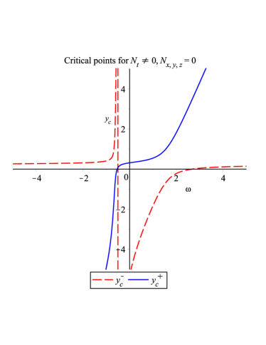
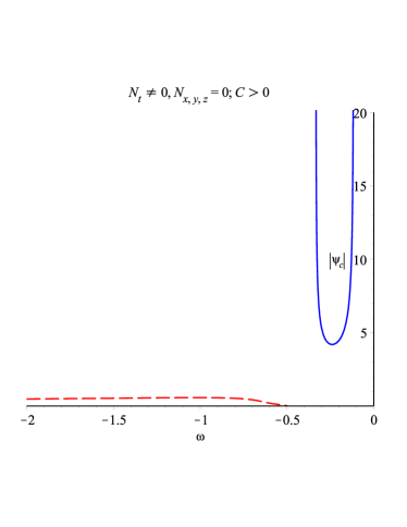
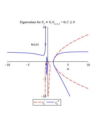
Figure 1: (a) Numeric values of the critical manifolds vs $\omega$ for $N_{t}=1,N_{x,y,z}=0,$ (b) Critical time trajectory of the anisotropy vs $\omega$ with repeller potential $C>0$ for $N_{t}=1,N_{x,y,z}=0,$ (c) Critical time trajectory of the Brans Dicke scalar field vs $\omega$ with repeller potential $C>0$ for $N_{t}=1,N_{x,y,z}=0$ and (d) Real part of eigenvalues vs $\omega$ for $N_{t}=1,N_{x,y,z}=0$ and $C\geq 0$

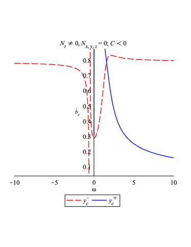
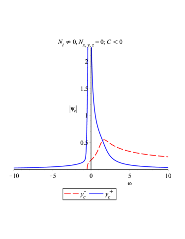
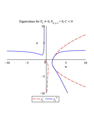
Figure 2: (a) Critical time trajectory of the anisotropy vs $\omega$ with absorber potential $C<0$ for $N_{t}=1,N_{x,y,z}=0,$ (b) Critical time trajectory of the Brans Dicke scalar field vs $\omega<0$ with absorber potential $C<0$ for $N_{t}=1,N_{x,y,z}=0$ (c) Eigenvalues for $N_{t}=1,N_{x,y,z}=0$ with attractor potential $C<0$

The above relations show that to have real fields, we should choose $C>0$ in limits $\omega\to\infty$ (see Eq.33) but for small regions of the $\omega$ parameter the case $C<0$ has still some acceptable solutions (see diagrams 2-a and 2-b). We plot diagrams of the critical solutions (26), (27), (28) and (29) versus the $\omega$ parameter in Figures 1 and 2 for $C=\pm 1$. In fact $C>0$ describes a repeller Brans Dicke potential while $C<0$ shows an attractor potential. Diagram of 1-a shows all possible real values for $y_{c}^{\pm}.$ Diagram of 1-b shows $\dot{b}_{c}$ versus $\omega$ parameter at critical manifolds $y_{c}^{\pm}.$ Diagram of the Figure 1-c shows variation of the $\psi_{c}$ versus $\omega$ parameter at points $y_{c}^{\pm}.$ However, time trajectories of the fields $H(t)$ and $\psi(t)$ are obtained by the linearized form of the equations (41) and (42) near the critical values $(H_{c},\psi_{c})$ as follows

$$\frac{d}{dt}\left(\begin{array}[]{c}H(t)\\ \psi(t)\\ \end{array}\right)=\left(\begin{array}[]{cc}J_{11}&J_{12}\\ J_{21}&J_{22}\\ \end{array}\right)\left(\begin{array}[]{c}H(t)\\ \psi(t)\\ \end{array}\right),$$ (36)

where the constants $J_{ij}=\frac{\partial\chi_{i}}{\partial q_{j}}$ with $\chi_{i}=\{\dot{H},\dot{\psi}\}$ and $q_{j}=\{H,\psi\}$ are components of the Jacobi matrix of two dimensional phase space $(H,\psi).$ They are calculated at the critical point $y_{c}$ by applying (41) and (42) as follows

$$J_{ij}=\frac{\psi_{c}}{2(1+2\omega)}\left(\begin{array}[]{cc}3\omega-6(1+2\omega)y_{c}&3\omega y_{c}-2\omega(15\omega+6)\\ 2(3-2\omega)&2(3-2\omega)y_{c}-2(2+\omega)\\ \end{array}\right),$$ (37)

which its secular equation $\det(J_{ij}-\sigma\delta_{ij})=0$ reads

$$(2+4\omega)^{2}\sigma^{2}+2(1+2\omega)[6(1+2\omega)\psi_{c}+2(2\omega-3)y_{c}+4-\omega]\sigma$$

$$+\psi_{c}[(48\omega^{2}-48\omega-36)y_{c}+24\omega^{2}+60\omega+24]-120\omega^{3}+126\omega^{2}+60\omega=0.$$ (38)

This secular equation has two different solutions versus the $\omega$ parameter and they occur at Figures 1-d and 2-c for $C\geq 0$ and $C<0$ respectively. In fact for $C\geq 0$ vertical axis in Figure 1-d shows real part of complex eigenvalues whose negative numeric values describe spiral stable nature for the system while negative numeric values in the vertical axis of the figure 2-c show stable nature for the system. These diagrams show just one negative numeric value for the eigenvalues for large $\omega$ and the second eigenvalue has not negative numeric value. This means that the system will be quasi stable for $\omega>>1.$ This can be follow by asymptotic behavior of the eigenvalues at $\omega\to\infty$ which are obtained from (3.1) as follows

$$\sigma_{1}^{\pm}\approx 0.016+2.74\sqrt{\omega}+O(\omega^{-1/2})>0,~{}~{}~{}for~{}~{}~{}y_{c}^{-}$$ (39)

and

$$\sigma_{2}^{\pm}\approx 0.016-2.74\sqrt{\omega}+O(\omega^{-1/2})>0,~{}~{}~{}for~{}~{}~{}y_{c}^{+}.$$ (40)

Diagrams of the eigenvalues in Figures 1-d and 2-c show stable nature for our parametric solutions just for numeric values of the $\omega$ parameter where all two eigenvalues take on negative numeric values. This occurs at small $\omega.$ For instance for ansatz $\omega=0.7$ with $C=+1$ we obtain numeric values for the critical points and corresponding eigenvalues as $y_{c}^{+}=0.45$ with $\sigma_{1}^{+}=-0.6+0.8i$ and $\sigma_{2}^{+}=0.2-3.5i$ and $y_{c}^{-}=-2.7$ with eigenvalues $\sigma_{1}^{-}=-0.7-1.7i$ and $\sigma_{2}^{-}=-1.8+0.9i.$ These critical points have $\psi^{+}_{c}=0.9i$ and $\psi_{c}^{-}=0.3i$ and so are not physical solutions because $\psi_{c}^{\pm}$ have imaginary numeric value and are not real fields. While one can check numeric values of the critical points for $\omega=0.7$ with attractor potential $C=-1$ to be physical as $y_{c}^{+}=0.5$ with corresponding values for $\psi^{+}_{c}=0.9$ and $\sigma_{1}^{+}=-1.5+1.6i$ and $\sigma_{2}^{+}=-1.5-1.6i$ which describes a spiral stable physical solution. And for second critical point $y_{c}^{-}=-2.7$ with $\psi_{c}^{-}=0.3$ and $\sigma_{1}^{-}=-1.7+1.6i$ and $\sigma_{2}^{-}=-1.7-1.6i$ which describes a spiral stable physical solution also. By looking at the series forms (32),(33) and (35) we must be choose $\omega<0(>0)$ for the case $C>0(<0)$ but (34) shows that for physical real fields we must be set just $C<0$ and so we collect some physical numeric solutions for the critical points and corresponding eigenvalues in the table 1 for different $\omega$ values. In the last column of the table we call stability nature of the physical (means with real fields for $y_{c}$ and $\psi_{c}$) solutions. To obtain numerical solutions given in the table 1 we set ansatz $C=-1.$

Table 1: critical points, eigenvalues and their nature for $C=-1$

$\omega$	$(y_{c}^{+},y_{c}^{-})$	$(\psi_{c}^{+},\psi_{c}^{-})$	$(\sigma_{1}^{+},\sigma_{2}^{+})$	$(\sigma_{1}^{-},\sigma_{2}^{-})$	$Nature$
$+\infty$	$(+\infty,0)$	$(0,0)$	$(+\infty,+\infty)$	$(-\infty,-\infty)$	quasi stable
+100	$(+263.02,-0.22)$	$(+0.003,+0.073)$	$(+2.88,-260.37)$	$(+29.64,-29,83)$	quasi stable
+0.9	$(+0.5,-2.1)$	$(+0.8,+0.4)$	$-1.3\pm 1.5I$	$-1.3\pm 1.6I$	spiral stable
+0.6	$(+0.4,-2.7)$	$(+0.96,+0.27)$	$-1.7\pm 1.6I$	$-2\pm 1.3I$	spiral stable
+0.5	$(+0.4,-3.3)$	$(+1.1,+0.25)$	$-1.8\pm 1.5I$	$-2.5\pm 0.56I$	spiral stable
+0.1	$(+0.3,-4.8)$	$(+8.7,+0.16)$	$(-1.3,-5.6)$	$(-0.67,-26.62)$	stable
0.0	$(+0.31,-5.3)$	$(+2.9,+0.17)$	$(-1,-8.7)$	$(-17.94,-0.52)$	stable
-0.1	$(+0.3,-6)$	$(+8.7,+0.16)$	$(-1.12,-26.34)$	(-0.4,-26.5)	stable
-0.5	$\infty$	$\infty$	$\infty$	$\infty$	undetermined
-0.6	$(+0.5,-0.4)$	$(+0.2,+3.3)$	$9.1\pm 10.8I$	$(-4.1-0.7I,-53.4+0.1I)$	spiral stable
-0.9	$(-0.4,+0.45)$	$(+0.15,+0.56I)$	$(+26.97,+1.51)$	$(+0.36-8.2I,+0.02+6.5I)$	un physical
-100	$(-270.3,0.22)$	$(+0.003,+0.07)$	$(+273.2,+2.8)$	$+0.02\pm 29.5I$	un stable
$-\infty$	$(-\infty,0)$	$(0,0)$	$(+\infty I,+\infty I)$	$(-\infty I,-\infty I)$	spiral quasi stable

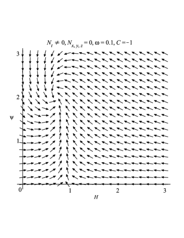
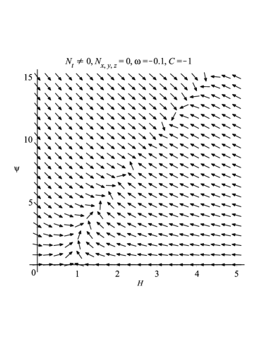
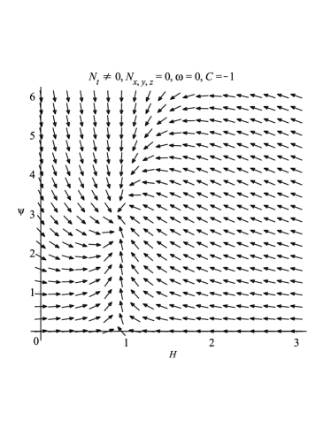
Figure 3: Arrow diagrams for attractor potential $C=-1$ for $\omega=0.1$ (a), $\omega=-0.1$ (b) and $\omega=0$ (c) in case $N_{t}\neq 0,N_{x,y,z}=0$

In fact, $y_{c}^{\pm}<0(>0)$ in the table 1 describe a collapsing (expanding) universe because physical values for critical time fluctuations of the Brans Dicke field $\psi_{c}$ should be take on some positive values and so negative numeric values for $y_{c}$ readds to a negative hubble parameter $H_{c}<0$ which describes a collapsing universe and so in the table 1 we should consider some real positive values for the fields $y_{c}^{\pm}>0$ and $\psi_{c}^{\pm}>0$ which are defined inflationary expanding universe. In fact $y_{c}^{\pm}>0$ given in the table 1 corresponds to a physical stable solution because both of corresponding eigenvalues take on negative numeric values. By looking at this, one can infer that for stable critical point the time trajectories of the Brans Dicke field should be a raising function which satisfies with physical situations. Because the Brans Dicke scalar field is inverse of the Newton‘s gravity coupling parameter by regarding the Mach‘s principle (see [61]). Also, one can see that for $C\geq 0$ the secular equation (3.1) give us a complex parametric eigenvalues and so to plot possible acceptable numeric values for the eigenvalues we must to plot real part of the complex parametric $\sigma(\omega)$ which are appeared in Figure 1-d. In the latter case one call spiral stable nature for the dynamical system under consideration with $Re(\sigma)<0$. According to the dynamical system approach (see [62]), we know that all possible stable solutions should have negative numeric values for the real eigenvalues and spiral stable nature for the solutions if the eigenvalues become complex number with negative numeric values for its real part. We plotted arrow diagrams of the dynamical field equations given by (23) and (24) in Figure 3 for choices $\omega=0$ and $\omega=\pm 0.1$ given by the table 1. These arrow diagrams show stable point where the arrows approach to a fixed point finally. This means stability of the metric solutions in studying of the dynamical system approach which show sink hole for $(H_{c},\psi_{c})>0.$ This is appeared for attractor potential $C=-1.$ However, one can solve (36) to obtain time trajectories of the fields $H(t)$ and $\psi(t)$ around the stable nature critical points $(H_{c},\psi_{c})$ given by the table 1 such that

$$H(t)=H_{c}+O_{H}(e^{\psi_{c}\sigma_{1}t}-e^{\psi_{c}\sigma_{2}t}),$$ (41)

and

$$\psi(t)=\psi_{c}+O_{\psi}(e^{\psi_{c}\sigma_{1}t}-e^{\psi_{c}\sigma_{2}t}),$$ (42)

in which $O_{H,\psi}$ are integral constants and they should be fixed with initial conditions on the system. In the above solutions, we choose origin of the time to be critical time $t_{c}=0$ for which $H(0)=H_{c}$ and $\psi(0)=\psi_{c}.$ Also, numeric values of the critical fields $H_{c}$ and $\psi_{c}$ for the stable critical points $y_{c}$ should be substituted by the numeric values in the table 1. By integrating the Equations (41) and (42), we obtain

$$a(t)=a_{c}+H_{c}t+\frac{O_{H}}{\psi_{c}\sigma_{1}}(e^{\psi_{c}\sigma_{1}t}-1)-\frac{O_{H}}{\psi_{c}\sigma_{2}}(e^{\psi_{c}\sigma_{2}t}-1),$$ (43)

and

$$\ln\bigg{(}\frac{\phi(t)}{\phi_{c}}\bigg{)}=\psi_{c}t+\frac{O_{\psi}}{\psi_{c}\sigma_{1}}(e^{\psi_{c}\sigma_{1}t}-1)-\frac{O_{\psi}}{\psi_{c}\sigma_{2}}(e^{\psi_{c}\sigma_{2}t}-1),$$ (44)

where we assumed

$$a(0)=a_{c},~{}~{}~{}\phi(0)=\phi_{c}.$$ (45)

We can substitute (41) into the definition of the deceleration parameter $-q=1+\frac{\dot{H}}{H^{2}}$ to obtain

$$q(t)\approx-1+\frac{\psi_{c}\sigma_{1}}{O_{H}}e^{-\psi_{c}\sigma_{1}t}$$ (46)

for $\sigma_{1}>\sigma_{2}$ and vice versa. Acceleration of the universe say us $q<0$ for both primordial inflation or late time inflation. At late time inflation (the present epoch of the anisotropic universe), the above time dependent deceleration parameter reaches to the following limit

$$\lim_{t\to\infty}q(t)=-1,$$ (47)

and for beginning of the primordial inflation we have

$$\lim_{t\to-\infty}q(t)\approx-1,$$ (48)

while for end of primordial inflation we can evaluate

$$q(0)=-1+\frac{\psi_{c}\sigma_{1}}{O_{H}}<0,$$ (49)

which reads

$$O_{H}>\psi_{c}\sigma_{1}$$ (50)

if $\sigma_{1}>\sigma_{2}$ and vice versa. In this view, we assumed that the primordial inflation is begin at $t\to-\infty$ for which isotropic part of space time scale factor vanishes $a(-\infty)=-\infty$ and it is ended at the time $t=0$ where at this duration of expansion the declaration parameter takes on some negative numeric values. By substituting (43) the equation $\dot{b}=Ke^{-3a}$ reads

$$\dot{b}(t)=K\exp\{-8a_{c}-8H_{c}t-\frac{8O_{H}}{\psi_{c}\sigma_{1}}(e^{\psi_{c}\sigma_{1}t}-1)+\frac{8O_{H}}{\psi_{c}\sigma_{2}}(e^{\psi_{c}\sigma_{2}t}-1)\},$$ (51)

in which for stable physical solutions we have $\sigma_{1,2}<0$ and $\psi_{c}>0$ and so the above anisotropy velocity decreases with $t\to\infty.$ By regarding the condition (50) the solutions (51) and (41) read to the following forms for numeric values of the critical point $\omega=0.1$ given in the table 1.

$$\dot{b}(t)=\exp\{-20.88-16\exp{(-11.31t)}+16\exp{(-48.72t)}\}$$ (52)

and

$$\dot{a}(t)=H(t)=2.61-22.62\exp{(-11.31t)}+22.62\exp{(-48.72t)}$$ (53)

where we set

$$K=e^{8a_{c}}, O_{H}=2\psi_{c}\sigma_{1}.$$ (54)

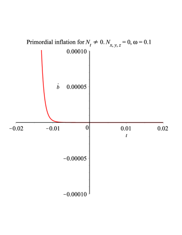
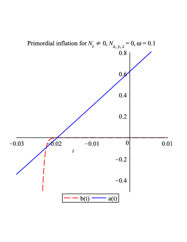
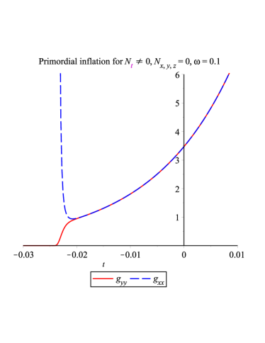
Figure 4: (a,b)Isotropic and anisotropic time trajectories and (c) isotropic and anisotropic scale factors and (d) directional metric components vs cosmic time $t$ for primordial inflation in case $N_{t}=1,N_{x,y,z}=0$ for stable solution $\omega=0.1$ given in the table 1

Diagrams of these solutions given in the Figure 4 show that velocity of anisotropy time trajectory of the space time $\dot{b}(t)$ is smaller than the Hubble parameter time trajectory (velocity of isotropy part of the space time) by raising the cosmic time but it dose not never vanishes. Now, we investigate some suitable conditions for the solutions (51) and (43) such that they can be satisfy both of primordial or late time inflations for line element (9).

3.1.1 Primordial inflation

In the primordial inflation, the scale factor of the space time (9) takes on smallest size and the system is in high energy state. Thus, one can assume that the background metric is flat Minkowski at duration of this phase of the expansion and so we should substitute boundary conditions $a(0)=a_{c}=0$ at end of the primordial inflation in the equations (54) such that

$$K=1,$$ (55)

$$b(t)\approx-\frac{e^{-1761(t-t_{p})}}{1761},$$ (56)

and

$$a(t)\approx 32.13(t-t_{p})+14.76(t-t_{p})^{2},$$ (57)

where $t_{p}=-0.01919308906$ is particular cosmic time for which $\dot{b}(t_{p})=1$ and to calculate the above integral solutions we use first order Taylor series expansion in the exponent of the functions $\dot{b}$ and $\dot{a}$ given by the equations (52) and (53). The solution (56) shows that for beginning of the primordial inflation $(t<<t_{p})$ the anisotropy of the space time is not negligible but is for late time inflationary phase of the space time expansion $(t>>t_{p})$. By substituting the solutions (56) and (57) into the definitions of the metric fields we obtain

$$g_{xx}=\exp\{64.26(t-t_{p})^{2}+29.52(t-t_{p})^{2}+0.0023\exp[-1761(t-t_{p})]\}$$ (58)

and

$$g_{yy}=g_{zz}=\exp\{64.26(t-t_{p})^{2}+29.52(t-t_{p})^{2}-0.001\exp[-1761(t-t_{0})]\}.$$ (59)

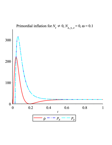
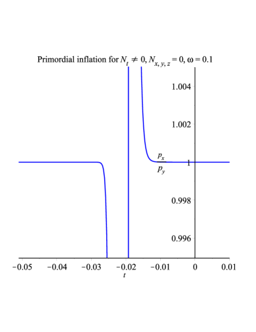
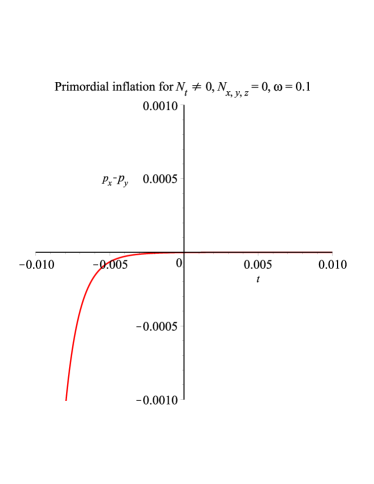
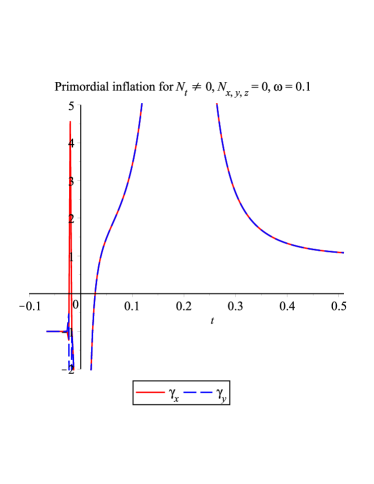
Figure 5: (a) Re-scaled density and directional pressures vs the dimensionless cosmic time $t$ and (b) directional barotropic indexes vs the dimensionless cosmic time $t$ for primordial inflation in case $N_{t}=1,N_{x,y,z}=0$

Diagrams of the solutions (52) and (53) are plotted in Figures 4-a and 4-b. Diagrams of the equations (56) and (57) are plotted in Figures 4-c and corresponding metric components of line element (9) are plotted in Figures 4-d. They show isotropic scale factor raises faster than the anisotropic scale factor and at duration of the inflation there is not more different time trajectories between $g_{xx}$ and $g_{yy}=g_{zz}$. For this stable solution, we obtain matter density, directional pressures and corresponding barotropic indexes which are defined by the following formulas and whose diagrams are plotted in Figures 5.

$$\frac{\rho(T)}{\rho_{c}}=G^{t}_{t}=3(a^{\prime 2}-b^{\prime 2}),$$ (60)

$$\frac{p_{x}}{\rho_{c}}=2a^{\prime\prime}+2b^{\prime\prime}+3a^{\prime 2}+6a^{\prime}b^{\prime}+3b^{\prime 2},$$ (61)

$$\frac{p_{y}}{\rho_{c}}=2a^{\prime\prime}-b^{\prime\prime}+3a^{\prime 2}-3a^{\prime}b^{\prime}+3b^{\prime 2},$$ (62)

in which

$$\prime\equiv\frac{d}{dT},~{}~{}~{}T=t\sqrt{\rho_{c}},~{}~{}~{}\rho_{c}=3(H_{c}^{2}-\dot{b}_{c}^{2}),$$ (63)

and barotropic indexes are obtained by

$$\gamma_{x}=\frac{p_{x}}{\rho},~{}~{}~{}\gamma_{y}=\frac{p_{y}}{\rho},~{}~{}~{}\bar{\gamma}=\frac{\gamma_{x}+2\gamma_{y}}{3},$$ (64)

where explicit form of time dependence of the above functions are not shown because they have long length. They do not show negative pressures for after the primordial inflation $t>0$ which means that the Brans Dicke scalar vector matter behaves as regular visible matter instead of dark sector for support of spacetime inflation. In fact the Figure 5-d shows that before end of primordial inflation $t\to 0$ we have $\gamma_{x,y}<0$ which means that the matter field of the model behaves as dark sector. Red line in the Figure 5-a shows the density of the matter has maximum point firstly and then reaches to a local minimum which means that in the end of the primordial inflation the system reaches to the reheating phase. But with the passage of time, it has tended to a very low density, which can be the average density of the current phase of the world by setting the observational data.Diagrams of 5-a and 5-b and 5-c show that anisotropy of the space time is negligible after end of the primordial inflation but not before than. In our calculations, we set the dimensionless parameters so that the end time of primordial inflation is zero. Now, in the next subsection we check the above general solutions for the late inflationary period.

3.1.2 Late inflationary period

In this approach, the spacetime scale is large and the anisotropic part of scale factor is negligible. In other word, the universe is old (the present state) and so, we can use the asymptotic solutions given by (43) such that for $t>>1$ we can write

$$a(t)\approx\ln N+H_{c}t,~{}~{}~{}b(t)\approx 0,$$ (65)

in which we defined e-folding parameter as

$$a_{c}=\ln N>>1.$$ (66)

In this regime, the line element (9) reaches to a flat Robertson Walker metric with scale factor $\exp(t\sqrt{\Lambda/3})$ in the asymptotic de Sitter epoch in which

$$\Lambda=3H_{c}^{2},$$ (67)

is effective cosmological constant which supports the exponential expansion of the universe. To determine $N$ value given by the identity (66), we should use the observational data. From the observational point of view, the total number of e-folds, must be larger than $N>60$, which depends on the scale of inflation and thermal history after inflation [73]. Also, for critical density of the matter we should use $\rho_{c}\approx 8.5\times 10^{-}{27}kg/m^{3}$ from observational data.
The scalar spectral index $n_{s}$ is observational quantity to check validity of our solutions. With lowest order terms it is defined by slow rolling parameters $|\epsilon|<1$ and $|\eta|<1$ of the inflation [74] as $n_{s}\simeq 1-6\epsilon+2\eta$ where $\epsilon=\frac{m_{p}^{2}}{16\pi}\big{(}\frac{\partial_{\phi}U(\phi)}{U(\phi)}\big{)}^{2}$ and $\eta=\frac{\partial_{\phi}^{2}U(\phi)}{U(\phi)}$ are defined versus the derivatives of the inflation potential. To match the observational data, at end of the inflation we should have $n_{s}\approx 1$. This will be guarantee the generation of scale invariant scalar perturbations. In fact, the Planck satellite full mission temperature data and a first release of polarization data on large angular scales measure the spectral index of curvature perturbations to be $n_{s}=0.968\pm 0.006$ [71]. By substituting the potential $U=C\phi$ given by (22), we obtain

$$\epsilon=\frac{m_{p}^{2}}{16\pi\phi^{2}},~{}~{}~{}\eta=0,~{}~{}~{}~{}n_{s}=1-\frac{3m_{p}^{2}}{8\pi\phi^{2}},$$ (68)

in which $m_{p}$ is the Planck mass. By substituting the solution (44) at limits $t\to>>\psi_{c}^{-1}$ the above relations reads

$$n_{s}=1-\frac{3m_{p}^{2}}{8\pi\phi_{c}^{2}}e^{-\psi_{c}t}\approx 1,$$ (69)

which obey observational conditions. In the next subsection, we investigate other possible metric solutions in case where the timelike dynamical vector field is parallel with the spatial symmetry axis of the Bianchi I line element (9).

3.2 Metric solution for $(N_{x}\neq 0,N_{t,y,z}=0)$

By substituting $N_{x}\neq 0,N_{t,y,z}=0,$ the equation (10) reduces to the following conditions.

$$\beta=0,~{}~{}~{}\alpha=\frac{i\pi}{2},~{}~{}~{}N_{x}=ie^{a-2b},$$ (70)

and the fields equations $\phi$, $N_{\mu}$ and $G_{\mu\nu}$ take on the following forms respectively.

$$2\omega\frac{\ddot{\phi}}{\phi}+2\omega(\dot{a}+4\dot{b})\frac{\dot{\phi}}{\phi}-\omega\frac{\dot{\phi}^{2}}{\phi^{2}}-18\dot{a}^{2}-86\dot{b}^{2}+108\dot{a}\dot{b}+2\ddot{a}+\frac{\partial U(\phi,N_{x})}{\partial\phi}=0,$$ (71)

$$\frac{\zeta}{\phi}=-102\dot{a}^{2}-20\dot{b}^{2}+216\dot{a}\dot{b}-8\ddot{a}+12\ddot{b}-24(\dot{a}-2\dot{b})\bigg{(}\frac{\dot{\phi}}{\phi}\bigg{)}-\frac{1}{\phi N_{x}}\frac{\partial U}{\partial N^{x}},$$ (72)

and $G_{t}^{t},G_{x}^{x},G_{y}^{y}=G_{z}^{z}$ will be respectively

$$\ddot{a}+\frac{\omega}{2}\frac{\dot{\phi}^{2}}{\phi^{2}}-10\dot{a}^{2}+58\dot{a}\dot{b}-69\dot{b}^{2}-\frac{U}{\phi}=0,$$ (73)

$$\ddot{a}-10\ddot{b}+830\dot{a}^{2}-136\dot{a}\dot{b}+111\dot{b}^{2}+9\dot{a}\bigg{(}\frac{\dot{\phi}}{\phi}\bigg{)}+\frac{\omega}{2}\frac{\dot{\phi}^{2}}{\phi^{2}}+3\frac{\ddot{\phi}}{\phi}+\frac{(U+\zeta)}{\phi}=0,$$ (74)

and

$$\frac{\omega}{2}\frac{\dot{\phi}^{2}}{\phi^{2}}+\frac{\ddot{\phi}}{\phi}+3\frac{\dot{a}\dot{\phi}}{\phi}+67\dot{b}^{2}-55\dot{a}\dot{b}+16\dot{a}^{2}+\frac{U(\phi,N_{x})}{\phi}=0.$$ (75)

The above five equations are enough to determine all fields $a,b,\phi,\zeta,U.$ By substituting (70) and definitions

$$\dot{a}=H,~{}~{}~{}\dot{b}=B,~{}~{}~{}\frac{\dot{\phi}}{\phi}=\psi,$$ (76)

we can write the following identities for potential.

$$\frac{1}{N_{x}}\frac{\partial U}{\partial N^{x}}=\frac{\partial U}{\partial a}-\frac{1}{2}\frac{\partial U}{\partial b}=\bigg{(}\frac{1}{H}-\frac{1}{2B}\bigg{)}\dot{U},~{}~{}~{}\frac{\partial U}{\partial\phi}=\frac{\dot{U}}{\phi\psi}.$$ (77)

By substituting (76) and (77) one can show that the dynamical field equations (71), (72), (73), (74) and (75) are transformed to the following first order nonlinear differential equations.

$$\dot{H}=\frac{(-\omega\phi\psi^{2}+138B^{2}\phi-116BH\phi+20H^{2}\phi+2U)}{2\phi},$$ (78)

$$\dot{\psi}=-\frac{(\omega\phi\psi^{2}+134B^{2}\phi-110BH\phi+32H^{2}\phi+6H\phi\psi+2\phi\psi^{2}-2U)}{2\phi},$$ (79)

$$\dot{B}=-\frac{(3\omega\phi\psi^{2}+42B^{2}\phi+58BH\phi-1584H^{2}\phi-10U-2\zeta)}{20\phi},$$ (80)

$$\dot{U}=\frac{2HB}{5(H-2B)}\times$$ (81)

$$(2986B^{2}\phi-11\omega\phi\psi^{2}-3226BH\phi-240B\phi\psi-3842H^{2}\phi+120H\phi\psi+10U-\zeta),$$ (82)

and

$$\zeta= \frac{5\psi[\omega^{2}\phi\psi^{2}+134B^{2}\omega\phi-8B\omega\phi\psi-52B^{2}\phi-2(\omega+1)U]}{H},$$

$$-\frac{5\psi(\omega^{2}\phi\psi^{2}+32H^{2}\omega\phi+4H\omega\phi\psi+2\omega\phi\psi^{2}-2H^{2}\phi-2(\omega+1)U)}{2B}$$

$$+2986B^{2}\phi-(885\omega\phi\psi+3226H\phi+70\phi\psi)B$$

$$+435H\omega\phi\psi+29\omega\psi^{2}\phi-3842H^{2}\phi+90H\psi\phi+10U.$$ (83)

By solving the equations $\dot{H}=0=\dot{\psi}=\dot{B}=\dot{U}$, we obtain critical points as follows

$$H_{c}=2B_{c},~{}~{}~{}\psi_{c}=2.2484B_{c},~{}~{}~{}U_{c}=-1557B_{c}^{2}\phi_{c},~{}~{}~{}\zeta_{c}=4B_{c}^{2}\phi_{c},~{}~{}~{}\omega=-618.77,$$ (84)

in which critical anisotropy velocity $B_{c}$ is arbitrary constant which should be determined by observational data. This shows that in order to have at least one metric solution, we must have an anisotropy at the critical point, that is, $B_{c}=\dot{b}_{c}\neq 0.$ To determine if the above critical manifolds show stable metric solution, we must be determine eigenvalues of the Jacobi matrix of the above dynamical field equations in four dimensional phase space $\{H,B,\psi,U\}$ similar to previous section by solving the corresponding secular equation. This fourth degrees algebraic equation has a negative real root (eigenvalues) such that

$$\sigma_{1}=\sigma_{2}=\sigma_{3}=\sigma_{4}=-269.1022666B_{c}.$$ (85)

Its negativity shows stable (unstable) nature for our obtained metric solutions in phase space with $B_{c}>0(B_{c}<0).$ By looking at the critical point (84) one can infer that similar to previous section this stable solution is supported with attractor critical potential $U_{c}=-1557B_{c}^{2}\phi_{c}.$ In fact, in the real universe we know that the anisotropy part of the metric field should be decreasing function and in large scales of the universe it is negligible. While for our solution the critical hypersurface $H_{c}=2B_{c}$ in phase space shows that anisotropy is not negligible and grows with half velocity of the isotropic expansion. Furthermore, in a real universe the Brans Dicke scalar field should be increasing function versus the cosmic times which for our critical solution is happened for $B_{c}>0$ with equation (84) as $\psi_{c}=2.2484B_{c}.$ This shows that our solution can be physical. Because in accordance with the Mach‘s principle the authors of the work [61] showed that the Brans Dicke gravity for a FRW cosmology predicts a raising function for the Brans Dicke scalar field which behaves as inverse of Newton‘s gravity coupling parameter. Such a asymptotic behavior for the Brans Dicke field obeyed by our obtained solution in this subsection. However, we now obtain time trajectories of the fields near the above stable critical point versus the eigenvectors (not shown) as follows

$$H(T)\approx 2B_{c}+H_{1}\exp(-269T),$$ (86)

$$\psi(T)\approx 2.2484B_{c}+\psi_{1}\exp(-269T),$$ (87)

$$B(T)\approx B_{c}+B_{1}\exp(-269T),$$ (88)

and

$$U(T)\approx\frac{41.672B_{c}^{3}\phi_{c}\exp(-269T)}{H_{1}-2B_{1}},$$ (89)

where we defined dimensionless cosmic time

$$T=B_{c}t,$$ (90)

and integral constants $H_{1},\psi_{1},B_{1}$ should be determined by observational data. By integrating the solutions (86), (87) and (88) we obtain time trajectory of the metric and the Brans Dicke scalar fields as follows

$$a(T)\approx a_{c}+2T-\frac{1}{269}\frac{H_{1}}{B_{c}}\exp(-269T),$$ (91)

$$\ln\bigg{(}\frac{\phi}{\phi_{c}}\bigg{)}\approx 2.2484T-\frac{1}{269}\frac{\psi_{1}}{B_{c}}\exp(-269T),$$ (92)

and

$$b(t)\approx b_{c}+T-\frac{1}{269}\frac{B_{1}}{B_{c}}\exp(-269T),$$ (93)

where $a_{c},b_{c},\phi_{c}$ are initial (critical) isotropic and anisotropic metric fields and the Brans Dicke scalar field which is given at begin of the inflation. For this solution the matter density $\rho=G^{t}_{t}=3(H^{2}-B^{2})$ and directional pressures $p_{x}=G_{x}^{x},~{}p_{y}=G_{y}^{y}$ read

$$\frac{\rho(T)}{B_{c}^{2}}=9+\frac{6(2H_{1}-B_{1})}{B_{c}}\exp(-269T)+\frac{3(H_{1}^{2}-B_{1}^{2})}{B_{c}^{2}}\exp(-538T).$$ (94)

$$\frac{p_{x}}{B_{c}^{2}}=27-\frac{520(H_{1}+B_{1})}{B_{c}}\exp(-269T)+3\bigg{(}\frac{H_{1}+B_{1}}{B_{c}}\bigg{)}^{2}\exp(-538T),$$ (95)

and

$$\frac{p_{y}}{B_{c}^{2}}=9-269\frac{(2H_{1}-B_{1})}{B_{c}}\exp(-269T)+3\bigg{(}\frac{H_{1}^{2}-H_{1}B_{1}+B_{1}^{2}}{B^{2}_{c}}\bigg{)}\exp(-538T).$$ (96)

To obtain admissible values of the constants ${H_{1},B_{1}}$, we calculate extremum point of the density and we consider this physical fact in which the matter density with all possible forms should have positive values for all times. To do so, we set $\frac{d\rho}{dT}=0$ and obtain

$$T_{m}=-\frac{1}{269}\ln\bigg{(}\frac{B_{c}(2H_{1}-B_{1})}{B_{1}^{2}-H_{1}^{2}}\bigg{)},~{}~{}~{}\rho_{m}=\rho(T_{m})=\frac{3B_{c}^{2}(2B_{1}-H_{1})^{2}}{B_{1}^{2}-H_{1}^{2}}.$$ (97)

For a physical stable metric solution where $B_{c}>0$ (see the eigenvalue) the above relations show that we should have

$$H_{1}<B_{1}<2H_{1},~{}~{}~{}(H_{1},B_{1})>0,$$ (98)

and

$$H_{1}>B_{1}>2H_{1},~{}~{}~{}(H_{1},B_{1})<0.$$ (99)

One can infer that (97) approaches to the following limits

$$\lim_{B_{1}\to H_{1}}(T_{m},\rho_{m})=(-\infty,+\infty),~{}~{}~{}\lim_{B_{1}\to 2H_{1}}(T_{m},\rho_{m})=(+\infty,9B_{c}^{2}),$$ (100)

in which left (right) side describes expanding (collapsing) Bianchi cosmology. By substituting $B_{1}=H_{1}$ the mass density and the pressures for expanding phase read

$$\frac{\rho(T)}{3B_{c}^{2}}=3+2\chi e^{-269T},~{}~{}~{}\chi=\frac{H_{1}}{B_{c}},$$ (101)

$$\frac{p_{x}(T)}{B_{c}^{2}}=27-1040\chi e^{-269T}+12\chi^{2}e^{-538T},$$ (102)

and

$$\frac{p_{y}(T)}{B_{c}^{2}}=9-269\chi e^{-269T}+3\chi^{2}e^{-538T}.$$ (103)

For collapsing (reheating) phase of the Bianchi I cosmology with $B_{1}=2H_{1},$ we can obtain time trajectories of mass density and directional pressures of the Bianchi I cosmology as follows

$$\frac{\rho(T)}{9B_{c}^{2}}=1-\chi^{2}e^{-538T},$$ (104)

$$\frac{p_{x}(T)}{3B_{c}^{2}}=9-520\chi e^{-269T}+9\chi^{2}e^{-538T},$$ (105)

and

$$\frac{p_{y}(T)}{9B_{c}^{2}}=1+\chi^{2}e^{-538T}.$$ (106)

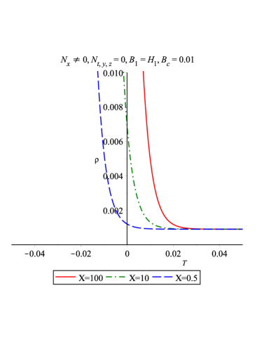
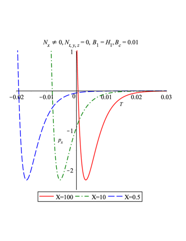
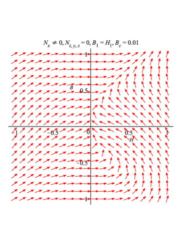
Figure 6: (a) Diagram of the density vs dimensionless cosmic time $T$ for $N_{x}\neq 0,~{}N_{t,y,z}=0,$ (b) pressure in $x$ direction is plotted vs $T$ for $N_{x}\neq 0,N_{t,y,z}=0,$ (c) Diagram of $y$ direction pressure is plotted vs $T$ for $N_{x}\neq 0,N_{t,y,z}=0$ and (d) Arrow diagrams for case $N_{x}\neq 0,N_{t,y,z}=0$ with sink hole nature.

We plot diagrams of the above functions for arbitrary values $B_{c}=0.01$, and $\chi=0.5,10,100$ respectively in Figure 6. We check that diagrams of the directional barotropic indexes (not shown) are similar to diagrams of the pressures but with re-scaled size. Negative regime of the pressures (or corresponding barotropic index) in the diagrams show a phase transition which originates from anisotropy velocity $B\neq 0$ while one can imagine that it is apparently originates from unknown dark sector matter. In other words the Brans Dicke scalar vector fluid behaves as dark sector of the cosmic matter. In Figure 6-d, one can see that arrow diagram of the metric fields in which arrows converge to a stable point with a non-vanishing anisotropy velocity $B\neq 0.$

3.3 Primordial inflation

Same as previous section we know that in primordial inflation the spacetime has smallest scale and is in high energy state such that we assume $a(0)=0=b(0)$ and then the metric solution (91), (93) read

$$a_{p}(T)=2T+\frac{\chi}{269}(1-e^{-269T}),~{}~{}~{}b_{p}(T)=T+\frac{\chi}{269}(1-e^{-269T}),$$ (107)

with constraint condition

$$a_{c}=b_{c}=\frac{\chi}{269}.$$ (108)

$$g_{xx}^{(p)}(T)=\exp\{-\frac{2\chi}{269}(1-e^{-269T})\},~{}~{}~{}g^{(p)}_{yy}=g^{(p)}_{zz}=\exp\{6T+\frac{4\chi}{269}(1-e^{-269T})\},$$ (109)

where superscript $(p)$ denotes $primordial.$ This metric solution shows at end of primordial inflation the spacetime reaches to non vanishing smallest scale in parallel direction with the cylindrical symmetry axis $x$ but in vertical direction $y=z$ the inflation continues to next phase such that

$$\lim_{269T>>1}g_{xx}\approx e^{-\frac{2\chi}{269}},~{}~{}~{}\lim_{269T>>1}g_{yy}=g_{zz}\approx e^{6T+\frac{4\chi}{269}}.$$ (110)

This means that at duration of the primordial inflation compression of spacetime is happened in direction of symmetry axis $x$ while expansion of space time is happened in its vertical directions $y,z$. In other words, primordial inflation in this model is similar to expansion of cigarette like or pipeline. By substituting (86) and definitions $B_{1}=H_{1}$ and $\chi=\frac{H_{1}}{B_{c}}$ into the deceleration parameter $q=-1-\frac{\dot{H}}{H^{2}}$ we obtain

$$q(T)=-1+\frac{269\chi\exp(-269T)}{[2+\chi\exp(-269T)]^{2}}.$$ (111)

It is easy to check that for end of primordial inflation the above deceleration parameter reduces to the following form

$$q_{e}=\lim_{269T>>1}q(T)\approx-1,$$ (112)

which satisfies the de Sitter epoch full but for beginning of the primordial inflation we have

$$q_{0}=q(0)=-1+\frac{269\chi}{(2+\chi)^{2}},$$ (113)

in which the beginning time of the primordial inflation is chosen to be $t_{c}=0.$ Negativity condition on the deceleration parameter at beginning of the primordial inflation shows the following restriction on the $\chi$ parameter.

$$q_{0}<0,~{}~{}~{}~{}-\infty<\chi<0.01509519949.$$ (114)

We assume at end of primordial inflation which is happened after passing times $T_{p}>>1,$ the anisotropy can be negligible and the metric components (110) reach to the following approximation

$$g_{xx}^{(p)}(T_{p})\approx g_{yy}^{(p)}(T_{p})\approx e^{N_{p}},$$ (115)

in which $N_{p}$ is e-folding parameter of the spacetime at end of the primordial inflation and so we can write

$$-\frac{2\chi}{269}=N_{p}=6T_{p}+4\frac{4\chi}{269}.$$ (116)

This identity gives out

$$T_{p}=-\frac{\chi}{269},~{}~{}~{}N_{p}=2T_{p}.$$ (117)

By applying these boundary conditions on our general metric solutions given by (91) and (93) we now obtain exact form of the solutions which satisfy the late time inflation.

3.4 Late inflationary period

In this case, the scale of the space time is large and so the anisotropy can be negligible and so the metric field solutions (91) and (93) will be

$$g^{(L)}_{xx}=\exp\{2a_{c}-4b_{c}+\frac{2\chi}{269}e^{-269T}\},$$ (118)

and

$$g^{(L)}_{yy}=g^{(L)}_{zz}=\exp\{2a_{c}+2b_{c}+6T-\frac{4\chi}{269}e^{-269T}\},$$ (119)

where superscript $(L)$ denotes $Late$. If we assume $T_{0}$ is beginning time of the late inflationary period in which anisotropy has more small effects we should use continuity condition of the metric fields at time $T_{0}$ as $g^{(L)}_{xx}(T_{0})=g_{yy}^{(L)}(T_{0})$ and equality of whose first derivative $\frac{dg_{xx}^{(L)}(T_{0})}{dT}=\frac{dg_{yy}^{(L)}(T_{0})}{dT}$ which by using the above solutions we obtain

$$b_{c}=-T_{0}-\frac{1}{269},~{}~{}~{}~{}\chi=-e^{269T_{0}}.$$ (120)

By substituting (120) into the metric field solutions (118) and (119) we have

$$g^{(L)}_{xx}=\exp\{2a_{c}+4T_{0}+\frac{2}{269}(2-e^{-269(T-T_{0})})\},$$ (121)

and

$$g^{(L)}_{yy}=g^{(L)}_{zz}=\exp\{2a_{c}-2T_{0}+6T-\frac{2}{269}(1-2e^{-269(T-T_{0})})\}.$$ (122)

By using the approximation $e^{-269(T-T_{0})}\approx 1-269(T-T_{0})$ we can rewrite the above metric solutions for the times $T>T_{0}$ such that

$$g_{xx}^{(L)}\approx g_{yy}^{(L)}=g_{zz}^{(L)}\approx e^{N+2(T-T_{0})},$$ (123)

where

$$N=2a_{c}+\frac{2}{269}+4T_{0},$$ (124)

is assumed to be the e-folding parameter of the late time inflation and it should be determined by observational data. We again remember that observations show that the current world is old enough such that the e-folding parameter should be a large number between $N\sim\{60\cdots 70\}.$ This asymptotic behavior of the metric solution (123) shows a homogenous and isotropic FRW spacetime in de Sitter epoch in which critical value of the anisotropy velocity $B_{c}$ behaves as an effective cosmological constant such that

$$2B_{c}=\sqrt{\frac{\Lambda}{3}},~{}~{}~{}T=B_{c}t.$$ (125)

However, $N$ is evaluated by observations but how can define the integral constant $a_{c}$ with other physical parameters of the system? To do so we assume $T_{0}=T_{p}$ and $N=N_{p}$ which means end of primordial inflation is continued with beginning of the late time inflation. By regarding this, one can infer

$$a_{c}=-\frac{1}{269}-2T_{p}.$$ (126)

We end this section by calculating the scalar spectral index [74]

$$n_{s}=1+2\eta-6\epsilon,$$ (127)

in which the slow rolling parameters of the inflation $\epsilon$ and $\eta$ mentioned in the previous section take on extended forms with two variable potential $U(\phi,N_{x})$ (two fluid model) as follows

$$\epsilon=\frac{m_{p}^{2}}{16\pi}\bigg{(}\frac{\partial_{\phi}U(\phi,N_{x})}{U}+\frac{\partial_{N^{x}}U(\phi,N_{x})}{\phi N_{x}U}\bigg{)}^{2},$$ (128)

and

$$\eta=\frac{m_{p}^{2}}{8\pi}\bigg{(}\frac{\partial_{\phi}^{2}U}{U}+2\frac{\partial_{N^{x}}\partial_{\phi}U}{\phi N_{x}U}+\frac{\partial^{2}_{N^{x}}U}{\phi^{2}N_{x}^{2}U}\bigg{)},$$ (129)

which by substituting (77) and chain derivative can be rewritten as follows

$$\epsilon=\frac{m_{p}^{2}}{16\pi}\bigg{(}\frac{1}{\psi}+\frac{1}{H}-\frac{1}{2B}\bigg{)}^{2}\frac{\dot{U}^{2}}{\phi^{2}U^{2}},$$ (130)

and

$$\eta= \frac{m^{2}_{p}}{8\pi}\bigg{\{}\bigg{(}\frac{1}{\phi\psi}+\frac{1}{H}-\frac{1}{2B}\bigg{)}^{2}\frac{\ddot{U}}{U}-\frac{\dot{U}}{U}\bigg{[}\frac{1}{\phi^{3}}+\frac{\dot{\psi}}{\phi^{2}\psi^{3}}+\bigg{(}\frac{2}{\phi\psi}+\frac{1}{H}-\frac{1}{2B}\bigg{)}\frac{\dot{H}}{H^{2}}$$

$$-\bigg{(}\frac{2}{\phi\psi}+\frac{1}{2H}-\frac{1}{4B}\bigg{)}\frac{\dot{B}}{B^{2}}\bigg{]}\bigg{\}}.$$ (131)

By substituting the critical point (84) and time dependent potential solution (89) we obtain asymptotic critical values for these slow rolling parameters such that

$$\epsilon_{c}\approx 0,~{}~{}~{}\eta_{c}\approx\frac{2}{\pi}\bigg{(}\frac{30m_{p}}{\phi_{c}}\bigg{)}^{2},$$ (132)

for which the scalar spectral index $n_{s}$ become

$$n_{s}\simeq 1+\frac{1}{\pi}\bigg{(}\frac{60m_{p}}{\phi_{c}}\bigg{)}^{2}.$$ (133)

In the above relations, we set critical point conditions $\dot{H}=0=\dot{B}=\dot{U}=\dot{\psi}.$ By regarding the observation data for the scalar spectral index $n_{s}\approx 1$, we infer that the following inequality should be obeyed between $\phi_{c}$ and the Planck mass.

$$\phi_{c}>>60m_{p}.$$ (134)

In the following section we investigate possible stable metric solutions when direction of spatial part of the vector field is in perpendicular to axis of symmetry of the spacetime.

3.5 Metric solution for $(N_{y}\neq 0,N_{t,x,z}=0)$

In this case, the equation (10) reduces to the following constraint.

$$\alpha=\frac{i\pi}{2},~{}~{}~{}\beta=\frac{\pi}{2},~{}~{}~{}\gamma=0,~{}~{}~{}N_{y}=ie^{a+b},$$ (135)

and the field equations $\phi$, $N_{\mu}$ and $G_{\mu\nu}$ reduce to the following formes respectively.

$$2\omega\frac{\ddot{\phi}}{\phi}+2\omega(\dot{a}-2\dot{b})\frac{\dot{\phi}}{\phi}-\omega\frac{\dot{\phi}^{2}}{\phi^{2}}-2\dot{a}^{2}-12\dot{b}^{2}-34\dot{a}\dot{b}+8\ddot{a}+\frac{\partial U(\phi,N_{y})}{\partial\phi}=0,$$ (136)

$$\frac{\zeta}{\phi}=-54\dot{a}^{2}-2\dot{b}^{2}-54\dot{a}\dot{b}-10\ddot{a}-8\ddot{b}-8(\dot{a}+\dot{b})\bigg{(}\frac{\dot{\phi}}{\phi}\bigg{)}-\frac{\partial U(\phi,N_{y})}{\phi N_{y}\partial N^{y}},$$ (137)

and $G_{t}^{t},G_{x}^{x},G_{y}^{y}=G_{z}^{z}$ will be respectively

$$\ddot{a}+\frac{\omega}{2}\frac{\dot{\phi}^{2}}{\phi^{2}}+6\dot{a}^{2}+3\dot{a}\dot{b}-2\dot{b}^{2}-\frac{U}{\phi}=0,$$ (138)

$$3\ddot{a}+2\ddot{b}+6\dot{a}^{2}+9\dot{a}\dot{b}+4\dot{b}^{2}-\frac{\omega}{2}\frac{\dot{\phi}^{2}}{\phi^{2}}-\frac{\ddot{\phi}}{\phi}-3\dot{a}\frac{\dot{\phi}}{\phi}-\frac{U(\phi,N_{y})}{\phi}=0,$$ (139)

and

$$3\ddot{a}-\ddot{b}+6\dot{a}^{2}+4\dot{b}^{2}-\frac{\zeta}{\phi}-3\dot{a}\frac{\dot{\phi}}{\phi}-\frac{\ddot{\phi}}{\phi}-\frac{\omega}{2}\frac{\dot{\phi}^{2}}{\phi^{2}}-\frac{U}{\phi}=0.$$ (140)

The above five equations are enough to determine all quantities $a,b,\phi,\zeta$ and $U(\phi,N_{y}).$ By substituting (135) and definitions

$$\dot{a}=H,~{}~{}~{}\dot{b}=B,~{}~{}~{}\frac{\dot{\phi}}{\phi}=\psi,$$ (141)

we obtain the following identities for the potential

$$\frac{1}{N_{y}}\frac{\partial U}{\partial N^{y}}=\frac{\partial U}{\partial a}+\frac{\partial U}{\partial b}=\bigg{(}\frac{1}{H}+\frac{1}{B}\bigg{)}\dot{U},~{}~{}~{}\frac{\partial U}{\partial\phi}=\frac{\dot{U}}{\phi\psi}.$$ (142)

By using (141) and (142) one can show that the dynamical field equations (136), (137), (138), (139) and (140) are transformed to the following first order nonlinear differential equations.

$$\dot{H}=\frac{(-\omega\phi\psi^{2}+4B^{2}\phi-6BH\phi-12H^{2}\phi+2U)}{2\phi},$$ (143)

$$\dot{B}=-\frac{(9BH\phi+\zeta)}{3\phi},$$ (144)

$$\dot{\psi}=\frac{(-6\omega\phi\psi^{2}+30B^{2}\phi-18BH\phi-36H^{2}\phi-9H\phi\psi-3\phi\psi^{2}+6U-2\zeta)}{3\phi},$$ (145)

and

$$\dot{U}=-\frac{HB(-15\omega\phi\psi^{2}+66B^{2}\phi+24B\phi\psi-18H^{2}\phi+24H\phi\psi+30U-5\zeta)}{H+B},$$ (146)

and

$$\zeta= 3(4B\omega^{2}\phi\psi^{3}+4H\omega^{2}\phi\psi^{3}-20B^{3}\omega\phi\psi-8B^{2}H\omega\phi\psi+4B^{2}\omega\phi\psi^{2}$$

$$+36BH^{2}\omega\phi\psi+3BH\omega\phi\psi^{2}+5B\omega\phi\psi^{3}+24H^{3}\omega\phi\psi+4H^{2}\omega\phi\psi^{2}+5H\omega\phi\psi^{3}$$

$$+22B^{3}H\phi-4B^{3}\phi\psi+62B^{2}H\phi\psi-6BH^{3}\phi+116BH^{2}\phi\psi+50H^{3}\phi\psi-4BU\omega\psi$$

$$-4HU\omega\psi+10BHU-8BU\psi-8HU\psi)/(-4B\omega\psi-4H\omega\psi+5BH).$$ (147)

Similar to previous sections we solve the equations $\dot{H}=0=\dot{B}=\dot{\psi}=\dot{U}$ to obtain five critical manifolds which they are collected in the following table.

$\omega$	x	y	p	q
-2.38189179	-0.81852617	-0.92679835	7.36673550	-1.45863725
0.82291508	-0.50652226	1.75767870	4.55870034	-0.70900689
2.41213514	-0.71882277	1.08689952	6.46940495	0.36855696
2.53481716	-0.06704170	-1.54604186	0.60337534	-186521838
0.50000000	-0.42183288	2.00000000	3.79649596	-1.19784076

where we defined

$$H_{c}=xB_{c},~{}~{}~{}\psi_{c}=yB_{c},~{}~{}~{}\zeta_{c}=p\phi_{c}B_{c}^{2},~{}~{}~{}~{}U_{c}=q\phi_{c}B_{c}^{2}.$$ (148)

Physical boundary conditions for an accelerating expanding universe let us to choose $H_{c}>0$ for which time trajectory of the Brans Dicke scalar field should be raising function versus the cosmic times and so we should choose $\psi_{c}>0.$ These conditions lead to say that physical critical manifolds given in the above table are just $(x,y)>0$ for $B_{c}>0$ or $(x,y)<0$ for $B_{c}<0.$ By regarding the latter conditions and by looking at the numerical values of the table, we infer that $\omega=\{-2.381891793,2.534817164\}$ are physical choices for which both of the dimensionless critical manifolds $x$ and $y$ have negative numeric values synchronously and with $B_{c}<0$ they satisfy the physical boundary conditions $(H_{c},\psi_{c})>0.$ To determine whether this critical point give stable metric solutions, we need to determine sign of the eigenvalues. This is done by solving the secular equation of the Jacobi matrix for the above dynamical field equations similar to the previous sections. By doing this, we obtain for eigenvalues

$$\frac{\sigma_{1}^{1}}{B_{c}}=0.1512854848, \frac{\sigma_{2}^{1}}{B_{c}}=40.08736104,$$ (149)

$$\frac{\sigma_{3}^{1}}{B_{c}}=4.811325390+1.938390681i, \frac{\sigma_{4}^{1}}{B_{c}}=4.811325390-1.938390681i,$$

for $\omega=-2.381891793$ and

$$\frac{\sigma_{1}^{1}}{B_{c}}=0.2146088815, \frac{\sigma_{2}^{1}}{B_{c}}=11.13107522,$$ (150)

$$\frac{\sigma_{3}^{1}}{B_{c}}=46294.82001, \frac{\sigma_{4}^{1}}{B_{c}}=-46288.47253,$$

for $\omega=2.534817164.$ It is easy to see that the critical point (149) shows spiral source (unstable) and (150) shows quasi stable nature for the metric solutions of this subsection because for the former case, real part of all eigenvalues have positive numeric values while for the latter case at least one of the eigenvalues has negative real value. Hence, we end this section by plotting arrow diagram just for the latter quasi stable solution in Figure 7.

4 Concluding remark

In this work, we used the modified Brans Dicke scalar vector tensor gravity to study anisotropic Bianchi I cosmology. We solved dynamical field equations for different directions of the timelike dynamical vector field which interacts nonminimally with the Brans Dicke scalar field and the metric field. We succeeded to obtain analytic metric field solutions for epoch of primordial and late time inflations. In this model, in phase of primordial inflation the space time expansion is similar to pipeline geometry while in the late time inflation expansion is isotropic de Sitter epoch asymptotically. Time trajectories for anisotropy part of the metric field and the Hubble parameter and the Brans Dicke scalar field are not negligible in the primordial inflation but are at the late inflationary period. In the late inflationary period, critical value of velocity of the anisotropy behaves as an effective cosmological constant which can be claimed that it is really origin of the unknown cosmological parameter. By applying dynamical system approach, we investigated stability conditions of the solutions and obtained stable (un stable) nature in phase space when spatial directions of the timelike vector field is parallel (perpendicular) to the axes of symmetry of the spacetime. Negativity sign of the barotropic index which can be considered apparently as characterization of dark matter/energy, is in fact depended to direction of the vector field in the 4 dimensional Bianchi I line element. It has positive (negative) numeric value when spatial components of the vector field is ( is not) eliminated. In fact, when spatial components of the vector field is parallel to the symmetry axis of the spacetime our metric solutions have two different branches. One branch describes accelerating expansion of a Bianchi I cosmology with a stable nature in phase space while the second branch which describes a collapsing metric solution with quasi stable nature can be considered as reheating phase of the expansion. As extension of this work, we like to study dynamics of reheating phase with more details of this SVT Brans Dicke Bianchi I cosmology in our next work.

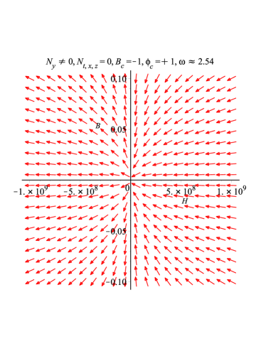
Figure 7: Arrow diagram for $N_{y}\neq 0,~{}N_{t,x,z}=0$ with quasi stable (saddle) nature

References

- [1] Liddle, L., & Lyth, D. 2000, Cosmological inflation and Large-Scale Structure, Cambridge University Press.
- [2] Hu, W., & Dodelson, S. 2002, Ann. Rev. Astron. Astrophys., 40, 171.
- [3] Dodelson, S. 2003, Modern Cosmology, Academic Press.
- [4] Weinberg, S. 2008, Cosmology, Oxford University Press.
- [5] Hutsemekers, D. 1998, Astronomy and Astrophysics, 332, 410.
- [6] Watkins, R., Feldman, H. A., & Hudson, M. J. 2009, Mon. Not. R. Astron. Soc., 391, 743.
- [7] Feldman, H. A., Watkins, R., & Hudson, M. J. 2010, Mon. Not. R. Astron. Soc., 407, 2328.
- [8] Macaulay, E., Feldman, H. A., Ferreira, P. G., Hudson, M. J., & Watkins, R. 2011, Mon. Not. R. Astron. Soc., 416, 621.
- [9] Longo, M. J. 2011, Phys. Lett. B, 699, 224.
- [10] Longo, M. J., astro-ph/0703325v3.
- [11] Longo, M. J., astro-ph/0707.3793.
- [12] Antoniou, I., & Perivolaropoulos, L. 2010, JCAP., 12, 012.
- [13] Cai, R. G., & Tou, Z. L. 2012, JCAP., 02, 004.
- [14] Yang, X., Wang, F. Y., & Chu, Z. 2014, Mon. Not. R. Astron. Soc., 437, 1840.
- [15] Chang, Z., & Lin, H. N. 2015, Mon. Not. R. Astron. Soc., 446, 2952.
- [16] Bengaly, C. A. P. Jr., Bernui, A. & Alcaniz, J. S. 2015, Astrophys. J., 808, 39.
- [17] Javanmard, B., Porciani, C., Kroupa, P., & Altenburg, J. P. 2015, Astrophys. J., 810, 47.
- [18] Webb, J. K., King, J. A., Murphy, M. T., Flambaum ,V. V., Carswell, R. F., & Bainbridge, M. B. 2011, Phys. Rev. Lett., 107, 191101.
- [19] King, J. A., Webb, J. K., Murphy, M. T., Flambaum, V. V., Carswell, R. F., Bainbridge, M. B., Wilczynska, M. R., & Koch, F. E. 2012, Mon. Not. R. Atron. Soc., 422, 3370.
- [20] Mariano, A., & Perivolaropoulos, L. 2012, Phys. Rev. D., 86, 083517.
- [21] Land, L., & Magueijo, J. 2007, Mon. Not. R. Astron., Soc., 378, 153.
- [22] Gruppuso, A., Finelli, F., Natoli, P., et al, 2011, Mon. Not. R. Astron. Soc., 411, 14445.
- [23] Hansen, H., Frejsel, A. M., Kim, J., Naselsky, P., & Nesti, F. 2011, Phys. Rev. D., 83, 103508.
- [24] Maris, M., Burigana, C., Gruppuso, A., Finelli, F., & Diego, J. M. 2011, Mon. Not. R. Astron. Soc., 415, 2546.
- [25] Ben-David, A., Kovetz, E. D., & Itzhaki, N. 2012, Astrophys. J., 748, 39.
- [26] Zhao, W., & Santos, L. 2015, The Universe, 3, 9.
- [27] Komatsu, E., et al, 2011, WMAP collaboration: Astrophys. J. Suppl., 192, 18.
- [28] Komatsu, E., et al, 2009, WMAP collaboration: Astrophys. J. Suppl. Ser., 180, 330.
- [29] Spergel, D. N., et al, 2007, WMAP collaboration: Astrophys. J. Suppl. Ser., 170, 377.
- [30] Peiris, H. V., et al, 2003, WMAP collaboration: Astrophys. J. Suppl. Ser., 184, 213.
- [31] Bennett, C. L., et al, 2003, WMAP collaboration: Astrophys. J. Suppl. Ser., 148, 1.
- [32] Bennett, C. L., et al, 2011, WMAP collaboration: Astrophys. J. Suppl., 192, 17.
- [33] Ade, P. A. R., et al, 2014, Planck Collaboration, Astron and Astrophys, 571, A23.
- [34] Ade, P. A. R., et al, 2016, Planck Collaboration, Astron and Astrophys, 594, A16.
- [35] Costa, A. O., et al, 2004, Phys. Rev. D., 69, 063516.
- [36] Schwarz, D. J., et al, 2004, Phys. Rev. Lett., 93, 221301.
- [37] Cruz, M., et al, 2007, Astrophys. J., 655, 11.
- [38] Hoftuft, J., et al, 2009, Astrophys. J., 699, 985.
- [39] Schwarz, D. J., Copi, C. J., Huterer, D., & Starkman, G. D. 2016, Class. Quantum. Grav., 23, 184001.
- [40] Akarus, O., & Kilinic, C. B. 2011, Int. J. Theor. Phys., 50, 1962.
- [41] Ellis, G. F. R. 2006, Gen. Relativ. Gravit, 38, 1003.
- [42] Golovnev, A., et al, 2008, J. Cosmol. Astropart. Phys., 06, 009.
- [43] Koivisto, T., & Mota, D. F. 2008, Astrophys. J., 679, 1.
- [44] Rodrigues, D. C. 2008, Phys. Rev. D., 17, 023534.
- [45] Koivisto, T., & Mota, D. F. A. 2008, J. Cosmol. Astropart. Phys., 08, 021.
- [46] Koivisto, T., & Mota, D. F. 2008, J. Cosmol. Astropart. Phys., 06, 018.
- [47] Akarus, O., & Kilinc, C. B. 2010, Gen. Relativ. Gravit., 42, 119.
- [48] Akarus, O., & Kilinc, C. B. 2010, Astrophys. Space Sci., 326, 315.
- [49] Akarus, O., & Kilinc, C. B. 2010, Gen. Relativ. Gravit., 42, 763.
- [50] Sharif, M., & Zubair, M. 2010, Astrophys. Space Sci., 330, 399.
- [51] Sharif, M., & Zubair, M. 2010, Int. J. Mod. Phys. D., 19, 1957.
- [52] Yadav, A. K., & Yadav, L. 2011, Int. J. Theor. Phys., 50, 218.
- [53] Kantowski, R., & Sachs, R. K. 1996, J. Math. Phys., 7, 443.
- [54] Brehme, R. W. 1997, Am. J. Phys., 45, 423.
- [55] Culetu, H. 2008, hep-th/0711.0062v3.
- [56] Campanelli, L., Cea, P., & Tedesco, L. 2006, Phys. Rev. Lett., 97, 131302.
- [57] Campanelli, L., Cea, P., & Tedesco, L. 2006, Phys. Rev. Lett, 97, 209903.
- [58] Campanelli, L., Cea, P., & Tedesco, L. 2007, Phys. Rev. D., 76, 063007.
- [59] Ghaffarnejad, H. 2008, Gen. Relativ. Gravit., 40, 2229.
- [60] Ghaffarnejad, H. 2009, Gen. Relativ. Gravit., 41(E), 2941.
- [61] Brans, C., & Dicke, R. 1961, Phys. Rev., 124, 925.
- [62] Ghaffarnejad, H., & Yaraie, E. 2017, Gen. Relativ. Gravit., 49, 49.
- [63] Ghaffarnejad, H. 2010, Class. Quantum. Grav., 27, 015008.
- [64] Ghaffarnejad, H. 2015, J. of Phys., Conf. series, 633, 012020.
- [65] Ghaffarnejad, H., & Dehghani, R. 2019, Eur. Phys. J. C., 79, 468.
- [66] Ghaffarnejad, H. 2019, J. of Phys. Conf. Series, 1391, 012028.
- [67] Will, C. M. 1993, Cambridge University press.
- [68] Will, C. M. 2006, Living Rev. Rel., 9.
- [69] Gaztanaga, E., & Lobo, J. A. 2001, Astrophys. J., 548, 47.
- [70] Reasenberg, R. D., et al, 1961, Astrophys. J., 234, 925.
- [71] Ade, P. A. R., et all, 2015, Planck Collaboration, Astron. and Astrophys., 594, 1.
- [72] Amirhashchi, H., & Yadav, A. K. 2020, Phys. of the Dark Universe, 30, 100711.
- [73] Kitajima, N., Tada, Y., & Takahashi, F. 2020, Phys. Lett. B., 800, 135097.
- [74] Coles, P., & Lucchin F. 1995, COSMOLOGY, The origin and Evolution of cosmic structure, John Wiley and Sons.
- [75] Linde, A., Linde, D., & Mezhlumian, A. 1994, Phys. Rev. D., 49, 1783.