Volumetric variational principles for a class of partial differential equations defined on surfaces and curves

Abstract

In this paper, we propose simple numerical algorithms for partial differential equations (PDEs) defined on closed, smooth surfaces (or curves). In particular, we consider PDEs that originate from variational principles defined on the surfaces; these include Laplace-Beltrami equations and surface wave equations. The approach is to systematically formulate extensions of the variational integrals, derive the Euler-Lagrange equations of the extended problem, including the boundary conditions that can be easily discretized on uniform Cartesian grids or adaptive meshes. In our approach, the surfaces are defined implicitly by the distance functions or by the closest point mapping. As such extensions are not unique, we investigate how a class of simple extensions can influence the resulting PDEs. In particular, we reduce the surface PDEs to model problems defined on a periodic strip and the corresponding boundary conditions, and use classical Fourier and Laplace transform methods to study the well-posedness of the resulting problems. For elliptic and parabolic problems, our boundary closure mostly yields stable algorithms to solve nonlinear surface PDEs. For hyperbolic problems, the proposed boundary closure is unstable in general, but the instability can be easily controlled by either adding a higher order regularization term or by periodically but infrequently ”reinitializing” the computed solutions. Some numerical examples for each representative surface PDEs are presented.

1 Introduction

This paper targets applications that use implicit or non-parametric representations of closed surfaces or curves and require numerical solution of certain partial differential equations defined on these surfaces. In immiscible multiphase fluids, surfactants can change important physical properties of the fluid mixture by lowering the tension of the fluid interface. The surfactant concentration satisfies a convection-diffusion equation in which the diffusion is described by a surface Laplacian of the concentration. This is a typical application in which the level set method enjoys an advantage in tracking the dynamically changing fluid interface. One of the challenges in developing a level set method for this application is in discretizing the surface Laplacian (Laplace-Beltrami) term, which typically requires some extension of the surfactant concentration and of the surface Laplacian operator into the ambient space somehow [34, 33, 35]. Eigenfunctions and eigenvalues of Laplace-Beltrami operator are of great interest and use in many scientific disciplines. In computer vision, eigenfunctions of the Laplace-Beltrami operator are used to compare and classify surfaces or solid objects [27, 28]. In differential geometry, solutions of the Laplace-Beltrami problem (Poisson’s equation on surfaces) can be used to find the Hodge decompositions of vector fields defined on the surfaces. The Hodge decomposition can be used to formulate boundary integral methods for problems in computational electromagnetic [14, 24].

We aim at developing a general mathematical framework for designing numerical schemes for solving a wide class of partial differential equations (PDEs) defined on closed manifolds that are not defined parametrically. The numerical schemes will inherit the flexibility of the level set method in dealing with such type of manifolds.

Let $\Omega\subset\mathbb{R}^{d}$ be a bounded open set with $C^{2}$ boundary $\Gamma=\partial\Omega$. For any small $\epsilon>0,$ define the narrowband of $\Gamma$ as

$$T_{\epsilon}=T_{\epsilon}(\Gamma):=\{z\in\mathbb{R}^{d}:\min_{x\in\Gamma}|z-x|<\epsilon\}.$$ (1.1)

In this paper, we consider integro-differential operators of the form

$$I_{\Gamma}[u]:=\int_{\Gamma}L(x,u(x),\nabla_{\Gamma}u(x))dS(x),$$ (1.2)

or

$$I_{\Gamma}[u]:=\int_{t_{1}}^{t_{2}}\int_{\Gamma}L(x,u(x,t),u_{t}(x,t),\nabla_{\Gamma}u(x,t))dS(x)dt,$$ (1.3)

and their extensions

$$\tilde{I}_{T_{\epsilon}}[v]:=\int_{T_{\epsilon}}\bar{L}(z,v(z),\nabla v(z))dz,$$ (1.4)

or

$$\tilde{I}_{T_{\epsilon}}[v]:=\int_{t_{1}}^{t_{2}}\int_{T_{\epsilon}}\bar{L}(z,v(z,t),v_{t}(z,t),\nabla v(z,t))dzdt.$$ (1.5)

We shall focus on partial differential equations arising from calculus of variations and develop an approach for finding critical points of $I_{\Gamma}[u]$, i.e.

$$\delta I_{\Gamma}[u]=0,$$

by solving

$$\delta\tilde{I}_{T_{\epsilon}}[v]=0.$$

Here $\delta I_{\Gamma}$ and $\delta\tilde{I}_{T_{\epsilon}}$ denote the variational derivatives of $I_{\Gamma}$ and $\tilde{I}_{T_{\epsilon}}$ in suitable function spaces, we shall further assume that $L$ and $\bar{L}$ are smooth functions. We first give some definitions that will facilitate the discussion.

Definition 1.1.

The closest point mapping $P_{\Gamma}:T_{\epsilon}\mapsto\Gamma$ is defined by

$$P_{\Gamma}z:=\mathrm{argmin}_{x\in\Gamma}|z-x|.$$ (1.6)

If more than one point of $\Gamma$ is equidistant to $x$, we shall randomly assign one of them as the definition of $P_{\Gamma}(z)$. Since $\Gamma$ is assumed to be $C^{2},$ $P_{\Gamma}$ is well-defined if $z$ is no farther than $\epsilon$ distance from $\Gamma$, for any $\epsilon\in[0,\kappa_{\infty}^{-1})$ where $\kappa_{\infty}$ is an upper bound of the curvatures of $\Gamma.$

If the distance function

$$d_{\Gamma}(z):=|P_{\Gamma}z-z|$$

is differentiable at $z$, then we have $P_{\Gamma}(z)=z-d_{\Gamma}(z)\nabla d_{\Gamma}(z).$

Definition 1.2.

Let $u$ be a function defined on $\Gamma$, its constant-along-normal extension or the closest point extension in $T_{\epsilon}$ is defined by $\bar{u}(z):=u(P_{\Gamma}z),\,\,\,\forall z\in T_{\epsilon}.$

Next we define equivalence among functions and functionals.

Definition 1.3.

Let $v$ be a function defined on $T_{\epsilon}$ and $u$ be a function defined on $\Gamma$. We say that $v$ is equivalent to $u$ if $v(z)=\overline{u}(z)\,\,\,\forall z\in T_{\epsilon}.$ In this case, we denote $v\equiv u$. Correspondingly, let $\tilde{I}_{T_{\epsilon}}$ and $I_{\Gamma}$ be two integral operators, we define $\tilde{I}_{T_{\epsilon}}\equiv I_{\Gamma}$ if

$$\tilde{I}_{T_{\epsilon}}[v]=I_{\Gamma}[u]\,\,\,\,\text{whenever\,\,\,\,}v\equiv u.$$ (1.7)

Naturally, we are interested in answering the questions:

Question.

Let $v(z)$ and $u(x)$ be respectively the solutions of the variational problems involving $\tilde{I}_{T_{\epsilon}}$ and $I_{\Gamma}$. If $\tilde{I}_{T_{\epsilon}}\equiv I_{\Gamma}$,

$$\text{{Is }}v\equiv u?$$

Moreover,

Question.

How stable is the equivalence against perturbation introduced by the numerical discretization? More precisely, how close is $\frac{\partial v}{\partial n}$ to zero?

Related work

Level set methods or the closest point methods

These methods extend the surface PDEs to ones in a narrowband $T_{\epsilon}$ around the surface $\Gamma$. The proposed work is motivated by various advantages and disadvantages of these methods. Of course the aim is to keep the advantages and get rid of the disadvantages. In the level set methods, e.g. [3, 10], partial derivatives on $\Gamma$, as well as on all nearby parallel surfaces $\Gamma_{\eta}$ (the collection of the points that are $\eta$ distance from $\Gamma$), are written in the form of the orthogonal projections of the gradient operator in the Euclidean space, and thus an equation in $T_{\epsilon}$ is defined formally replacing the surface gradient $\nabla_{\Gamma}u$ by $(I-\mathbf{n}\otimes\mathbf{n})\nabla v^{\epsilon}$. As a reminder, $v^{\epsilon}$ is a function defined in $T_{\epsilon}$. The closest point methods for solving parabolic and elliptic PDEs defined on surfaces, see e.g. [29, 19], assume the constant-along-normal extension of quantities defined on the surface, and replace surface gradient operator $\nabla_{\Gamma}$ by the gradient operator $\nabla$ defined in the embedding Euclidean space. Thus the methods typically involve iterations of (a) enforcing the constraint that solutions are constant-along-normal, $\overline{v^{\epsilon}}(z):=v^{\epsilon}(x)$ for $P_{\Gamma}z=x$, done by extensive interpolation, and (b) solution of the PDEs in $T_{\epsilon}.$ In either methods, the solution to a given surface PDE is extracted from the restriction of $v^{\epsilon}$ on $\Gamma$, via interpolation. Compared to the level set methods, the closest point methods can be applied more easily to manifolds of different co-dimensions and involve simpler differential operators. However, these two methodologies seem to be designed exclusively for solving initial value problems with explicit time stepping.

Finite element methods on arbitrary surfaces

A straightforward way to formulate finite element methods to solve the Laplace-Beltrami problem, $\Delta_{\Gamma}u=f$, on smooth surfaces $\Gamma=\partial\Omega$ involve: (i) approximate $\Omega$ by a polyhedron $\Omega_{h}$ such that $\Gamma$ is approximated by $\Gamma_{h,}=\partial\Omega_{h}$ which consists of collection of triangles whose vertices are on $\Gamma$; (ii) use $\Gamma_{h}$ to parametrize $\Gamma$ locally; (iii) extend the source term $f$ constant along the normal direction of $\Gamma$ to obtain an equivalent source function $f_{h}$ define on $\Gamma_{h}$; (iv) solve the weak form on $\Gamma_{h}$ by using standard finite element methods [9, 7, 8]. Linear finite elements with piecewise linear triangular approximation $\Gamma_{h}$ is discussed in [9]. For higher order finite element methods, $\Gamma$ is approximated by $\Gamma_{h}^{k}$, a collection of images of piecewise interpolating polynomial defined on each triangle of $\Gamma_{h}$, and use higher order elements defined on $\Gamma_{h}^{k}$ [7, 8]. These methods require nontrivial lifting and projection between $\Gamma_{h}^{k}$ and $\Gamma$ when evaluating integrals in weak form defined on $\Gamma_{h}^{k}.$ Other approaches approximate surface $\Gamma$ without using nodes on $\Gamma$ directly. For example, the trace finite element method [23] or sharp interface method and narrowband method [6], are designed when the surface $\Gamma$ is given by the zero level set of a function $\phi$ (not necessary a signed distance function). The level set function $\phi$ is first approximated by the nodal interpolant $\phi_{h}$. The approximate surface $\Gamma_{h}$ or neighborhood of $\Gamma$ are computed from the zero level set or $\epsilon$-neighborhood of $\phi_{h}$. Other qualities such as normal of $\Gamma$ and close map on $\Gamma$ are obtained from $\phi_{h}$ approximately. These methods share the same features: (i) alter the surface $\Gamma$ to an approximate surface $\Gamma_{h}$; (ii) change the variational form on $\Gamma$ to an equivalent variational form on $\Gamma_{h}$. However, the implementation of the equivalent weak form can be very complicated. Recently Olshanskii and Safin proposed a narrowband unfitted finite element method to solve elliptic PDEs defined on surfaces [21]. In their work, the surface PDE is replaced by an equivalent PDE on the narrowband $T_{\epsilon}(\Gamma)$ and an “equivalent” PDE is derived from the constant-along-normal extension of the solution without considering an approximate surface $\Gamma_{h}.$ The Neumann boundary condition for unfitted element is treated by a piecewise planar approximation to $\partial T_{\epsilon}$ as proposed in [2]. Some local subdivisions may be needed for the elements that are closed to the boundary. This work is closest to our formulation. However, as we shall describe below, our approach does not require adaptive meshing and allows a very general set of meshing of the ambience space. Both finite difference and finite element methods can be easily used for discretization.

Computation of the distance function, the closest point mapping and constant-along-normal extensions

The computation of the signed distance functions as well as the closest point mappings from given level set functions are by now considered standard component in the level set methods [26], and can be carried out to high order accuracy in many different ways, e.g. [30, 1, 36, 5], where by extending the interface coordinates as constants along interface normals, $P_{\Gamma}$ can be computed easily to fourth order in the grid spacing. Once an accurate distance function is computed on the grid, its gradient can be computed by standard finite differencing or by more accurate but wider WENO stencils [15]. If the surfaces are given initially by explicitly parameterized patches, fast algorithms such as the one proposed in [31] in combination with KD-Tree can be used.

The proposed framework

The proposed framework contains a theoretically sound formulation that admits unique solutions which are constant-along-normal, i.e. $v^{\epsilon}(z)=v(P_{\Gamma}z)$ for all $z\in T_{\epsilon}$, without enforcing extra constraints. The formulation will include relatively simple differential operators and a theory on suitable and easy to implement boundary conditions. As a result, the proposed method can easily be applied to solve problems involving curves and surfaces in three dimensions, integral constraints and eigenvalues — all of which pose some level of difficulty for the other methods. Some of the operators in the equations resulting from the proposed framework will resemble those used in [12, 21, 32]. However, the way the equations are derived, the boundary conditions, and the numerical methods differ significantly. We also propose a method to extend the wave equation on surface in volumetric form and treat the Neumann boundary condition in an easy way. The instability due to the approximation of boundary condition can be corrected by modifying the extended PDE.

In summary, the proposed method provides a unifying approach to tackle a wide range of problems defined on surfaces or curves in three dimensions. The reasons for considering the proposed framework are simple: the extended problems are easier to solve computationally, in particular for applications where the surfaces and curves are given non-parametrically and are changing dynamically, and/or some global information about the operators such as the eigenvalues and eigenfunctions needs to be computed. The variational integrals used in the formulation, discussed in Section 2, provide a natural and systematic way of investigating important issues on boundary conditions, regularization and compatibility. The proposed method also opens up possibility of direct numerical minimization methods for problems involving more nonlinear and degenerate surface equations. However, this direction will be investigated in a future paper.

Notations for finite difference discretization

In this paper, we shall use the following notations and setup for discussion involving finite difference discretization of the proposed equations and boundary conditions. Approximation of an unknown function $u$ will be constructed on the uniform Cartesian grid $h\mathbb{Z}^{2}$ for some $h>0$, and the typical notation $u_{i,j}$ for approximation of $u(ih,jh)$. For evolution problems, $u_{i,j}^{n}$ will denote the approximation for $u(ih,jh,n\Delta t)$ where $\Delta t$ is the step size and $n$ is a positive integer. We shall also use the standard notations for finite difference operators acting on the grid function $u_{i,j}$:

$$D_{\pm}^{x}u_{i,j}=\pm\frac{u_{i\pm 1,j}-u_{i,j}}{h},D_{\pm}^{y}u_{i,j}=\pm\frac{u_{i,j\pm 1}-u_{i,j}}{h}.$$

These finite difference operators, $D_{+}^{x},D_{-}^{x},D_{+}^{y}$ and $D_{-}^{y}$, are used to construct finite difference approximations of higher order partial derivatives of $u$. Polynomials of these four operators correspond to applying the operators recursively to the grid function as defined by the polynomials: e.g.

$$D_{+}^{x}D_{-}^{x}u_{i,j}=D_{+}^{x}\frac{u_{i,j}-u_{i-1,j}}{h}=\frac{u_{i+1,j}-2u_{i,j}+u_{i-1,j}}{h^{2}}$$

is a standard approximation of $u_{xx}(ih,jh)$, and

$$(D_{+}^{x}D_{-}^{x})^{2}u_{i,j} =D_{+}^{x}D_{-}^{x}(\frac{u_{i+1,j}-2u_{i,j}+u_{i-1,j}}{h^{2}})$$

$$=\frac{1}{h^{2}}D_{+}^{x}D_{-}^{x}u_{i+1,j}-\frac{2}{h^{2}}D_{+}^{x}D_{-}^{x}u_{i,j}+\frac{1}{h^{2}}D_{+}^{x}D_{-}^{x}u_{i-1,j}$$

is an approximation of $u_{xxxx}(ih,jh).$

Layout of the paper

This paper is organized as follows. In Section 2, we describe the proposed extensions and boundary closure for discretization of the extended problems on Cartesian grids or more general meshes. In Section 3, we consider minimization of strictly convex functionals which lead to elliptic equations. In Section 4, we study least-action principles that lead to hyperbolic problems. In both Sections 3 and 4, we study the stability of the proposed extensions under the presence of perturbation to the boundary (and initial) conditions. A brief summary of our findings is presented in Section 5. In the Appendix, we provide some details on the derivation of the operators used in the paper.

2 The proposed framework

In our framework, the closest point projection $P_{\Gamma}$ is used to define extension of integrants as well as to provide a change of variables for integration in the narrowband $T_{\epsilon}$. In extending a variational problem defined on $\Gamma$ to one defined in $T_{\epsilon}$, one needs to deal with the additional degrees of freedom in the co-dimensions of $\Gamma$: depending on the nature of $I_{\Gamma}$, one may need to do nothing, impose restrictions, adding a regularizing term specific to the additional dimension(s) or convexifying the resulting functional. Additionally, one needs to develop efficient stable numerical methods for enforcing suitable boundary conditions.

2.1 Extensions of functionals defined on closed surfaces of co-dimension one

We start with the general procedure proposed in [17] for integration on closed hypersurfaces. The procedure starts by rewriting the integral on $\Gamma$ using nearby parallel curves or surfaces. It is useful to have the following notation:

Definition 2.1.

Let $d_{\Gamma}$ be a signed distance function to $\Gamma=\partial\Omega$; i.e. $d_{\Gamma}(w)<0$ for any $w\in\Omega$ and $d_{\Gamma}(w)>0$ for any $w\in\bar{\Omega}^{c}.$ The “parallel surface” which is of $\eta$ distance from $\Gamma$ is denoted by

$$\Gamma_{\eta}:=\{y\in\mathbb{R}^{d}:d_{\Gamma}(y)=\eta\}.$$

The closest point projection $P_{\Gamma}$ is a diffeomorphism between $\Gamma$ and $\Gamma_{\eta}$ for any $\eta\in[0,\kappa_{\infty}^{-1})$ where $\kappa_{\infty}$ is an upper bound of the curvatures of $\Gamma$.

The integrals on the parallel curves or surfaces, indexed by the distance to $\Gamma$, are then averaged using a kernel $K_{\epsilon}\in C([-\epsilon,\epsilon])$ that satisfies $\int_{-\epsilon}^{\epsilon}K_{\epsilon}(\eta)\,d\eta=1$. We summarize the two steps as follows:

$$\int_{\Gamma}L(x)dS(x)=\int_{\Gamma_{\eta}}L(P_{\Gamma}y)J(y)dS(y)=\int_{-\epsilon}^{\epsilon}K_{\epsilon}(\eta)\int_{\Gamma_{\eta}}L(P_{\Gamma}y)J(y)dS(y)\,d\eta.$$ (2.8)

Here, $J$ is the Jacobian that comes from the change of variables $z\mapsto P_{\Gamma}z\in\Gamma$. For curves embedded in $\mathbb{R}^{2}$, $J(z)$ is given by

$$J(z)=1-d_{\Gamma}(z)\kappa(z),$$

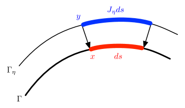
Figure 1: Parameterization of $\Gamma$ by a nearby parallel surface that is $\eta$ distance away.

where $\kappa$ is the curvature of the parallel curve $\Gamma_{\eta}$ that passes through $z$; i.e. $\eta=d_{\Gamma}(z)$. See Figure 1 for an illustration. Similarly, for surfaces embedded in $\mathbb{R}^{3}$, $J(z)$ is give by

$$J(z)=\prod_{j=1}^{2}[1-d_{\Gamma}(z)\kappa_{j}(z)]=\sigma_{1}(z)\sigma_{2}(z),$$ (2.9)

where $\kappa_{1},\kappa_{2}$ are the two principle curvatures of the parallel surface $\Gamma_{\eta}$ that passes through $z$. In [18], we show that $\sigma_{j}$ are the two largest singular values of $DP_{\Gamma}$, the derivative of the closest point projection operator. Thus $J(z)$ can be easily computed by finite differencing $P_{\Gamma}z$ and singular value decomposition.

Finally, by the coarea formula, see e.g. [11], the double integral on the right hand side of (2.8) equals to a Lebesque integral in $T_{\epsilon}$, and thus

$$\int_{\Gamma}L(x)dS(x)=\int_{T_{\epsilon}}L(P_{\Gamma}z)\,K_{\epsilon}(d_{\Gamma}(z))J(z)\,dz.$$

If $L$ depends on a function $u:\Gamma\mapsto\mathbb{R}$, there is no difficulty in applying the same extension procedure:

$$L(x,u(x))\longrightarrow L(P_{\Gamma}z,u(P_{\Gamma}z)).$$

Now if $L$ depends on $\nabla_{\Gamma}u$, the gradient of a function $u$ on $\Gamma$, one could apply the same procedure as above if there is a convenient formula for the constant-along-normal extension of $\nabla_{\Gamma}u(x).$ Naturally, we would like to relate the normal extension of the surface gradient $\overline{\nabla_{\Gamma}u}(z)$ to the gradient of the normal extension $\nabla_{z}\overline{u}(z)$ for $z\in T_{\epsilon}.$

We consider a simple motivating example involving concentric circles.

Example 2.2.

Let $\Gamma_{\eta}$ be the circle, centered at the origin, with radius $r_{0}+\eta$ for some $r_{0}>0$. Let $\bar{u}$ be a $C^{1}$ function on $\mathbb{R}^{2}\setminus\{(0,0)\}$. Consider polar coordinates $(r,\theta)$. On $\Gamma_{\eta}$, the derivative of $\bar{u}$ with respect to the arc length is related to that with respect to the angle $\theta$ by

$$\frac{\partial\bar{u}}{\partial s}=\frac{\partial\bar{u}}{\partial\theta}\frac{1}{r_{0}+\eta}.$$

Thus the curve derivative of $\bar{u}$ on $\Gamma$ is equivalent to the that on $\Gamma_{\eta}$, weighted properly by $J^{-1}:$

$$\frac{\partial\bar{u}}{\partial s}|_{\Gamma}=\frac{1}{r_{0}}\frac{\partial\bar{u}}{\partial\theta}=\frac{r_{0}+\eta}{r_{0}}\frac{\partial\bar{u}}{\partial s}|_{\Gamma_{\eta}}=J^{-1}\frac{\partial\bar{u}}{\partial s}|_{\Gamma_{\eta}}.$$

We can furthermore rewrite this equality into a general formula involving $\nabla\bar{u}$, the gradient of $\bar{u}$ in $\mathbb{R}^{2}$, and tangential and normal vectors, $\mathbf{t}$ and n, of the concentric circles:

$$\frac{\partial\bar{u}}{\partial s}|_{\Gamma}=J^{-1}(\nabla\bar{u}\cdot\mathbf{t})\mathbf{t}+\mu(\nabla\bar{u}\cdot\mathbf{n})\mathbf{n}=\left(J^{-1}\mathbf{t}\otimes\mathbf{t}+\mu\mathbf{n}\otimes\mathbf{n}\right)\nabla\bar{u},$$

for any $\mu.$ ∎

It can be shown easily that the surface gradient $\nabla_{\Gamma}u$, when embedded as a vector in $\mathbb{R}^{3}$, satisfies

$$\overline{\nabla_{\Gamma}u}(z)=A(z;\mu)\nabla_{z}\overline{u}(z),$$ (2.10)

where $A(z;\mu)=A_{0}(z)+\mu A_{1}(z),$

$$A_{0}(z):= \sigma_{1}^{-1}\mathbf{t}_{1}\otimes\mathbf{t}_{1}+\sigma_{2}^{-1}\mathbf{t}_{2}\otimes\mathbf{t}_{2},$$

$$A_{1}(z):= \mathbf{n}\otimes\mathbf{n},$$

and $\mathbf{t}_{1}$, $\mathbf{t}_{2}$ are the two orthonormal tangent vectors corresponding to the directions that yield the principle curvatures of $\Gamma$, $\mathbf{n}$ is the unit normal vector, $\mu$ can be any real number, and $\sigma_{1},$$\sigma_{2}$ are defined in (2.9). Thus $A_{0}$ corresponds to a weighted orthogonal projection onto the tangent plane and $A_{1}$ the projection along the normal of the parallel surface passing through $z.$ See Appendix for detail. The projection $\mu A_{1}\nabla_{z}\overline{u}(z)$ is always zero since $\overline{u}(z)$ is constant long the normal of $\Gamma$. The constituents of $A(z;\mu)$ can be easily computed from either the eigenvalues and eigenvectors of of $DP_{\Gamma}$ or $D^{2}d_{\Gamma}$; see [18].

In this paper, we consider extensions of $I_{\Gamma}[u]$ in the form:

$$\tilde{I}_{T_{\epsilon}}[v]:=\int_{T_{\epsilon}}\underbrace{L(P_{\Gamma}z,v(z),A_{0}\nabla v(z)+\mu A_{1}\nabla v(z))\,K_{\epsilon}(d_{\Gamma}(z))J(z)}_{\bar{L}(z,v,\nabla v)}\,dz,$$ (2.11)

where $\mu A_{1}\nabla v$ is the additional term corresponding to the extra degree of freedom in the co-dimension. If $I_{\Gamma}[u]$ is convex, the term $\mu A_{1}\nabla v$ should convexify the extended problem to ensure existence and uniqueness of the minimizer, and together with the natural boundary condition at $\partial T_{\epsilon}$ it should ensure that the minimizer satisfies Assumption 2.7. We refer to this additional term as the regularization term in $\tilde{I}_{T_{\epsilon}}$. The degree of freedom from the co-dimension needs to be treated differently for the saddle-point problem discussed in Section 4.

Also in this paper, we shall consider $K_{\epsilon}=\frac{1}{2\epsilon}\chi_{[-\epsilon,\epsilon]}$ for simplicity. The operator $\tilde{I}_{T_{\epsilon}}$ is equivalent to the original operator $I_{\Gamma}$. Instead of finding the minimizer of the energy $I_{\Gamma}[\cdot]$ in a Banach space of functions defined on $\Gamma$, we look for the minimizer of $\tilde{I}_{T_{\epsilon}}[\cdot]$ in a suitable Banach space of functions defined in $T_{\epsilon}$. The derivatives involved in $\tilde{I}_{T_{\epsilon}}[v]$ are in the Eulerian coordinates and therefore are easier to compute numerically. The geometry information of $\Gamma$ is embedded in the coefficient $A(z;\mu)$ and the boundary of $T_{\epsilon}$. We have been keeping the discussion on the relevant function spaces at minimum. In general, the choice of the function spaces for the extended problems depends on the specific problem class.

2.2 Extensions of functionals defined on closed surfaces of co-dimension two

In this paper, we only consider the extension for functionals defined on closed curves embedded in $\mathbb{R}^{3}.$ The procedure for integrating hypersurfaces is generalized in [18] to this case, with the the Jacobian

$$J(z)=\frac{\sigma_{1}(z)}{2\pi d_{\Gamma}(z)}.$$ (2.12)

Notice that the division by $d_{\Gamma}$ accounts for the fact that we are approximating a line integral (integration along $\Gamma$) by a family of surface integrals (integration on $\Gamma_{\eta},$ $\eta\in(0,\epsilon]$). We may remove this singularity by taking $K_{\epsilon}(\eta)=2\pi\eta\tilde{K}_{\epsilon}(\eta),$ $\tilde{K}_{\epsilon}\in C^{p}([0,\epsilon])$ and obtain

$$\int_{\Gamma}u(x)dS(x)=\frac{1}{Z_{0}}\int_{0}^{\epsilon}K_{\epsilon}(\eta)\int_{\Gamma_{\eta}}u(P_{\Gamma}z)\frac{\sigma_{1}(z)}{2\pi\eta}dS(z)\,d\eta=\frac{1}{Z_{0}}\int_{T_{\epsilon}}u(P_{\Gamma}z)\tilde{K}_{\epsilon}(d_{\Gamma}(z))\sigma_{1}(z)\,dz,$$

where $Z_{0}=\int_{0}^{\epsilon}K_{\epsilon}(\eta)d\eta$ is the normalizing factor.

Finally, the projection tensor in (2.10) has two degrees of freedom, and takes the from:

$$A(z;\mu_{1},\mu_{2}):=\left(\sigma_{1}^{-1}\mathbf{t}_{1}\otimes\mathbf{t}_{1}+\mu_{1}\mathbf{n}_{1}\otimes\mathbf{n}_{1}+\mu_{2}\mathbf{n}_{2}\otimes\mathbf{n}_{2}\right),$$

where $\mu_{1},\mu_{2}$ are two parameters corresponding to regularization in the co-dimensions to the curve, and $\sigma_{1}$ is the largest singular value of $DP_{\Gamma}(z).$

2.3 Equivalence between the minimizers of surface energy $I_{\Gamma}$ and its extension $\tilde{I}_{T_{\epsilon}}$

To justify our proposed method, we must demonstrate that $v\equiv u$ whenever $I_{\Gamma}\equiv\tilde{I}_{T_{\epsilon}}$. For simplicity, we only discuss the strictly convex energy

$$I_{\Gamma}[u]=\int_{\Gamma}L(x,u(x),\nabla_{\Gamma}u(x))dS(x).$$

Saddle point type energy is discussed in Section 4.

Theorem 2.3.

Suppose $\Gamma$ is a $C^{2}$-surface in $\mathbb{R}^{3}$ and $L(x,q,\mathbf{p}):\Gamma\times\mathbb{R}\times\mathbb{R}^{3}\rightarrow\mathbb{R}$ is twice continuously differentiable and satisfies $L_{\mathbf{p}}(x,q,\mathbf{t})\cdot\mathbf{n}(x)=0$ for and vector $\mathbf{t}$tangent to $\Gamma$ at $x$. Let $u$ be a $C^{2}$-solution of the Euler-Lagrange equation for surface energy $I_{\Gamma}$, $\delta I_{\Gamma}[u]=0$. Then its normal extension $\overline{u}:=u(P_{\Gamma}\cdot)$ is a solution of the Euler-Lagrange equation for extended energy $\tilde{I}_{T_{\epsilon}}$; i.e. $\delta\tilde{I}_{T_{\epsilon}}[\bar{u}]=0$, and $\bar{u}$ satisfies the Neumann boundary condition on $\partial T_{\epsilon}$.

Proof.

Since $u$ is a solution of the Euler-Lagrange equation $\delta I_{\Gamma}[u]=0$, $u$ satisfies

$$-\nabla_{\Gamma}\cdot L_{{\bf p}}(x,u,\nabla_{\Gamma}u)+L_{q}(x,u,\nabla_{\Gamma}u)=0\,\,\forall x\in\Gamma.$$ (2.13)

By Theorem A.1 in the Appendix, we have

$$\begin{split}\begin{split}\delta\tilde{I}_{T_{\epsilon}}[\bar{u}]=&-\nabla\cdot(JAL_{{\bf p}}(P_{\Gamma}z,\bar{u},A\nabla\bar{u}))+JL_{q}(P_{\Gamma}z,\bar{u},A\nabla\bar{u})\\ =&J(-J^{-1}\nabla\cdot(JAL_{{\bf p}}(P_{\Gamma}z,\overline{u},\overline{\nabla_{\Gamma}u}))+L_{q}(P_{\Gamma}z,\overline{u},\overline{\nabla_{\Gamma}u}))\\ =&J(-J^{-1}\nabla(\cdot JA\overline{L_{{\bf p}}(x,u,\nabla_{\Gamma}u)})+\overline{L_{q}(x,u,\nabla_{\Gamma}u)})\\ =&J(-\overline{\nabla_{\Gamma}\cdot L_{{\bf p}}(x,u,\nabla_{\Gamma}u)}+\overline{L_{q}(x,u,\nabla_{\Gamma}u)})=0\end{split}\end{split}$$ (2.14)

Therefore $\bar{u}$ satisfies the Euler-Lagrange equation for the extended energy $\tilde{I}_{T_{\epsilon}}$. It is obvious that $\frac{\partial\bar{u}}{\partial n}=0$ on $\partial T_{\epsilon}$ since it is true inside $T_{\epsilon}$ as well. ∎

Corollary 2.4.

If the normal extension of a function $u$ on $\Gamma$ satisfies $\delta\tilde{I}_{T_{\epsilon}}[\bar{u}]=0$, then $u$ is a solution of $\delta I_{\Gamma}[u]=0$.

Proof.

This follows from the proof in Theorem 2.3 directly. ∎

Corollary 2.5.

If the Euler-Lagrange equation $\delta I_{\Gamma}[u]=0$ is solvable and $\delta\tilde{I}_{T_{\epsilon}}[v]=0$ with the Neumann boundary condition has the unique solution $v$, then $v$ is constant-along-normal and $v_{\Gamma}$, the restriction of $v$ on $\Gamma$, is the unique solution of $\delta I_{\Gamma}[u]=0$.

Proof.

Let $u$ be a solution of $\delta I_{\Gamma}[u]=0$. Then by Theorem 2.3, $\overline{u}$ is a solution for $\delta\tilde{I}_{\Gamma}[v]=0$ with Neumann boundary condition. By uniqueness, we conclude that $v=\overline{u}$. Hence $v$ is constant-along-normal and $\delta I_{\Gamma}[u]=0$ has exactly one solution as well. ∎

Example 2.6.

The Laplace-Beltrami equation on $\Gamma$ reads as

$$-\Delta_{\Gamma}u=f\,\text{on}\,\Gamma,$$ (2.15)

and its extension in $T_{\epsilon}$ is

$$-\nabla\cdot(JA^{2}\nabla v)=\overline{f}J\,\,\text{on}\,\,T_{\epsilon},\,\,\frac{\partial v}{\partial n}=0\,\,\text{on}\,\,\partial T_{\epsilon}.$$ (2.16)

Since $\int_{T_{\epsilon}}\overline{f}\,Jdz=\int_{\Gamma}f\,dS$, the solvability for both equations are the same. We convexify the extended energy by using a positive constant $\mu$ in $A(z;\mu)$. The solution is unique up to an additive constant for both the original and extended problems. Therefore a solution of (2.16) is a normal extension of some solution of (2.15). In the weak formulations, the solution space for (2.15) is usually chosen to be $H^{1}(\Gamma)$ with zero mean, and the solution space for (2.16) is usually chosen to be $H^{1}(T_{\epsilon})$ with zero mean.

2.4 Boundary closure

In the previous two subsections, we derive the integral operators $\tilde{I}_{T_{\epsilon}}$ which are equivalent to $I_{\Gamma}$. The integral $\tilde{I}_{T_{\epsilon}}[v]$ or it’s variational derivative and the accompanying boundary conditions will be discretized. In this paper, we consider meshes that do not follow the geometry, in particular Cartesian grids, and unavoidably, we need to address the issue of discretization near the boundary $\partial T_{\epsilon}$. More specifically, near $\partial T_{\epsilon}$ numerical approximation of partial derivatives of $v$ will involve “ghost-values” on some “ghost nodes” lying outside of $T_{\epsilon}$ In this section, we describe a boundary closure procedure that works specifically to our setup.

Assumption 2.7.

The solution to the extended problem, $\tilde{I}_{T_{\epsilon}}[v]=\bar{f}$ or $\delta\tilde{I}_{T_{\epsilon}}[v]=0$ with suitable boundary conditions, satisfies

$$\frac{\partial v}{\partial n}:=\mathbf{n}\cdot\nabla v\equiv 0\,\,\,\text{in}\,\,\,T_{\epsilon},$$

where $\mathbf{n}(z)=\nabla d_{\Gamma}(z)$ is the normal vector of $\Gamma$ at $P_{\Gamma}z.$

We illustrate the essential idea of the proposed boundary closure by finite difference methods in the left subfigure of Figure 2. In the subfigure, the red nodes, also called as ghost nodes, are outside of $T_{\epsilon}$ but they are needed as part of the finite difference stencil for some blue nodes inside $T_{\epsilon}.$ We need to assign values to these red nodes in order to close the discretized system that contains only the interior blue nodes. We propose that:

• Each ghost node will be projected along the respective normal line back into a cell close to $\partial T_{\epsilon}$. In the figure, one of such cells is outlined in blue.

• An interpolation is performed using the grid values surrounding the blue cell. The order of interpolation must be higher or equal to the order used in discretization of the PDE on $T_{\epsilon}.$ The higher order interpolation the wider stencil as well as the wider narrowband.

Figure 2 shows an illustration of the boundary closure procedure that we implemented for an ellipse.

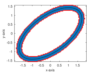
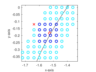
Figure 2: (Left) Illustration of computational domain when $\epsilon=3h$ and $h=1/25$. Black curve is the ellipse $\Gamma$, blue nodes are inner grids and red nodes are ghost nodes. (Right) The red x represents a ghost nodes and the red diamond represents the projected node we use to compute the value on the ghost node. Notice that, unlike the close point methods, ghost nodes do not need to be projected back to $\Gamma$. The nearby 16 dark blue nodes are used to interpolate the projected node.

Super-convergence of the boundary closure

We briefly explain why the proposed boundary closure can replace zero Neumann boundary conditions at $\partial T_{\epsilon}$. For simplicity, we demonstrate the two dimensional case. Let $(x_{i},y_{j})$ be a ghost node lying outside of $T_{\epsilon}$ and $(x_{i}^{\alpha},y_{j}^{\alpha})=(x_{i},y_{j})-\alpha\mathbf{n}_{i,j}$ be the projected node inside $T_{\epsilon}$ for some $\alpha>0$ of order $h$. Let $v_{i,j}^{\alpha}:=v(x_{i}^{\alpha},y_{j}^{\alpha})$ , then

$$v_{i,j}=v_{i,j}^{\alpha}\iff\frac{v_{i,j}-v_{i,j}^{\alpha}}{\alpha}=0,$$

which may be considered as a first order approximation of the zero Neumann boundary condition at $(x_{i}^{*},y_{j}^{*}):=(x_{i},y_{j})-\theta\mathbf{n}_{i,j}\in\partial T_{\epsilon}$ for some $0\leq\theta<\alpha.$ We extend the solution constant-along-normal further from $\partial T_{\epsilon}$ and assume that the extended $v$ is still smooth (for this we need to require that $\epsilon+2h<\kappa_{\infty}$). This means that

$$\frac{\partial v}{\partial\mathbf{n}}(x_{i}^{*},y_{j}^{*})=\frac{v_{i,j}-v_{i,j}^{\alpha}}{\alpha}+\frac{1}{2}(\alpha-2\theta)\frac{\partial^{2}v}{\partial\mathbf{n}^{2}}(x_{i}^{*},y_{j}^{*})+\mathcal{O}(h^{2}).$$

However, if $v$ satisfies Assumption 2.7, $\frac{\partial^{p}v}{\partial\mathbf{n}^{p}}(x_{i}^{*},y_{j}^{*})=0$, $p=1,2,\cdots$, we see that there is no error in the boundary closure.

In the procedure described above, $v_{i,j}^{\alpha}$ is then approximated to sufficient order of accuracy by interpolation. This will perturb the boundary condition to be of the form

$$\frac{\partial v}{\partial\mathbf{n}}\approx h^{k-1}\frac{\partial^{k}v}{\partial\mathbf{t}^{k}}+...$$

for some positive integer $k\geq 1$. It is not hard to argue that the proposed boundary closure yields convergent approximations of the solution to the given PDE with zero Neumann boundary conditions. But it is not so trivial to show that the convergence is high order for pure boundary value problems or evolution problems discretized by implicit schemes.

In particular, if we use bi-cubic interpolation centered at grid cell containing $(x_{i}^{\alpha},y_{j}^{\alpha})$ to approximate $v_{i,j}^{\alpha}$, simple calculations shows that the leading error in the approximation of $v_{i,j}^{\alpha}$ is of the form $h^{4}(c_{1}\frac{\partial^{4}u}{\partial x^{4}}+c_{2}\frac{\partial^{4}u}{\partial y^{4}})$ with positive coefficients $c_{1}$ and $c_{2}$. After a change of coordinates, and assuming that $v$ satisfies Assumption 2.7, the perturbed the boundary condition is given by

$$\frac{\partial v}{\partial\mathbf{n}}=ch^{3}\frac{\partial^{4}v}{\partial\mathbf{t}^{4}}+\text{(lower order in $h$ terms)}$$ (2.17)

with some positive coefficient $c$. In Section 3.1, we will see that the sign of $c$ plays an important role in stability of the proposed method.

Depth of projected points

We briefly discuss how to choose a suitable projection “depth” $\alpha>0$. Let ${\bf x}$ be a ghost node and ${\bf x}^{\alpha}={\bf x}-\alpha{\bf n}$ be the projected node inside $T_{\epsilon}$. When $v$ is constant-along-normal, any point along the normal direction has the same value of $v$. However, in numerical experiments, we need to choose a suitable projected node. The necessary condition for choosing the projected node is that the nearby surrounding nodes used to interpolate the value of $v$ must be inside $T_{\epsilon}$. In our numerical simulations, we use cubic interpolating polynomials in a dimension-by-dimension fashion to approximate $v({\bf x}^{\alpha})$. Hence it requires $4^{3}$ nearby points for 3 dimensional cases ($4^{2}$ nearby points for 2 dimensional case). See Figure 2 for illustration for a two dimensional case. We suggest that the projection depth be as shallow as possible. Therefore in our numerical simulation, we choose $\alpha=d_{\Gamma}(x)-(\epsilon-2\sqrt{d}h),$ which guarantees that the interpolation stencil stays inside $T_{\epsilon}$ if $\epsilon=mh$, $h<1/m\kappa_{\infty}$ and $m>2.$ Here $\kappa_{\infty}$ is an upper bound of the curvatures of $\Gamma$. We discuss the effect of different $\alpha$ in the examples in Section 3.4.1.

3 Minimization of convex energies

In this section, we shall first study a simple model problem defined on a flat torus. Such study will reveal many essential properties of the proposed algorithms, in particular, the stability of the extended problem, the consistency of the extended gradient flow.

3.1 Study of a model problem

Let $\Gamma$ to be the unit interval on the $x$-axis with periodic boundary conditions at $x=0$ and $1$, and $T_{\epsilon}=[0,1)\times(-\epsilon,\epsilon).$ For any $f\in C([0,1))$ with $f(0)=f(1)$ and $c>0$, we consider the energy

$$I_{\Gamma}[u]:=\int_{\Gamma}\frac{1}{2}(|\nabla_{\Gamma}u|^{2}+cu^{2})-fu\,dS=\int_{\Gamma}\frac{1}{2}(|u_{x}|^{2}+cu^{2})-fu\,dx,$$

and its extension (with $R(v_{y})=v_{y}^{2}$)

$$\tilde{I}_{T_{\epsilon}}[v]:=\int_{-\epsilon}^{\epsilon}K_{\epsilon}(y)\left(\int_{0}^{1}\frac{1}{2}(|v_{x}|^{2}+\mu v_{y}^{2}+cv^{2})-\bar{f}v\,dx\right)\,dy.$$

The Euler-Lagrange equation of $I_{\Gamma}$ is

$$-u_{xx}+cu=f,\,\,\,0<x<1,\,\,\,\text{and}\,\,u(0)=u(1),u^{\prime}(0)=u^{\prime}(1).$$ (3.18)

The Euler-Lagrange equation of $\tilde{I}_{T_{\epsilon}}$ and the natural boundary conditions for $v\in C^{2}(T_{\epsilon})$ are

$$-v_{xx}-\mu v_{yy}+cv=\bar{f}\,\,\,\text{in}\,T_{\epsilon},\,\,\,\,\,v(0,y)=v(1,y),v_{x}(0,y)=v_{x}(1,y)$$ (3.19)

$$v_{y}(x,\pm\epsilon)=0,\,\,\,0\leq x<1.$$ (3.20)

Here, we make a few observations for the case of $\mu>0$:

• $\tilde{I}_{T_{\epsilon}}[v]$ is strictly convex, and the Euler-Lagrange equation (3.19) of $\tilde{I}_{T_{\epsilon}}$ is uniformly elliptic, and has a unique solution in $C^{2}(T_{\epsilon})$ with the Neumann boundary condition (3.20).

• The $y$-derivative of the minimizer of $\tilde{I}_{T_{\epsilon}}$ has to be 0, for otherwise, $\tilde{I}_{T_{\epsilon}}$ can still take smaller values by diminishing $v_{y}^{2}$.

• For any function $\tilde{v}$ satisfying $\tilde{v}_{y}\equiv 0$ in $T_{\epsilon},$ $\tilde{I}_{T_{\epsilon}}[\tilde{v}]=I_{\Gamma}[\tilde{v}(\cdot,0)].$ Consequently, we can argue that $u(x):=v(x,0)$ is the minimizer of $I_{\Gamma}$, the solution of the corresponding Laplace-Beltrami equation.

3.1.1 Stability of the constant-along-normal solutions

We investigate this issue in three regards: (i) whether the interpolation used in the boundary closure introduces unstable solutions, and (ii) for time dependent problem, whether perturbation to the initial conditions will be amplified in time, and (iii) the effect of the inhomogeneous term not being perfectly constant-along-normal.

We study these issues with Example (3.1), involving (3.19), with $c>0$.

$$\frac{\partial v}{\partial y}=\begin{cases}\alpha\frac{\partial^{k}v}{\partial x^{k}},&y=\epsilon,\\ 0,&y=-\epsilon.\end{cases}$$ (3.21)

Due to linearity of the problem, the solution is a sum of a particular solution and the homogeneous solution ($f\equiv 0$) with perturbed boundary conditions. Therefore, we need to make sure that there exists no unstable homogeneous solution.

After Fourier transform in the $x$ variable, (3.19) and (3.21) become

$$\mu\hat{v}_{yy}(\omega,y)=(\omega^{2}+c)\hat{v}(\omega,y),\,\,\,\omega\in 2\pi\mathbb{Z},\,\,\,y\in(-\epsilon,\epsilon),$$

$$\frac{\partial\hat{v}}{\partial y}=\begin{cases}\alpha(i\omega)^{k}\hat{v},&y=\epsilon,\\ 0,&y=-\epsilon.\end{cases}$$

The general solution of this two-point boundary value problem takes the form

$$\hat{v}(\omega,y)=c_{1}e^{\kappa y}+c_{2}e^{-\kappa y},\,\,\,\kappa=\sqrt{\frac{\omega^{2}+c}{\mu}}>0.$$

We first observe that if there is a non-trivial solution, then the magnitude of $\kappa\epsilon=\sqrt{\frac{\omega^{2}+c}{\mu}}\epsilon$ determines an upper bound of the solution’s $y$-derivative, which translates to how far the solution is from being constant-along-normal. We only need to make sure that the non-trivial solution exists when $|\omega|$ is asymptotically smaller than $\epsilon^{-1}$.

From the boundary conditions at $y=\pm\epsilon$, we obtain

$$c_{1}\kappa e^{-\kappa\epsilon}-c_{2}\kappa e^{\kappa\epsilon} =0,$$

$$c_{1}\kappa e^{\kappa\epsilon}-c_{2}\kappa e^{-\kappa\epsilon} =\alpha(i\omega)^{k}(c_{1}e^{\kappa\epsilon}+c_{2}e^{-\kappa\epsilon}),$$

After simplification, we obtain

$$\kappa\,\tanh(2\kappa\epsilon)=\alpha(i\omega)^{k},$$ (3.22)

when $c_{1},c_{2}\neq 0$. We see that the existence of solutions to the eigenvalue problem (3.22) can be classified according to $k$ being an even or odd positive integer.

$k$ is odd.

We see that in this case there exists no solution to the eigenvalue problem (3.22). Therefore the only solution is the trivial solution $\hat{v}=0.$

$k$ is even.

More explicitly, the left hand side of equation (3.22) is

$$L(\omega):=\sqrt{\frac{\omega^{2}+c}{\mu}}\tanh\left(2\sqrt{\frac{\omega^{2}+c}{\mu}}\epsilon\right)$$

and the right hand side

$$R(\omega):=\tilde{\alpha}\omega^{k},$$

where $\tilde{\alpha}=i^{k}\alpha$. If $\tilde{\alpha}\leq 0$, $L(\omega)=R(\omega)$ has no solution. If $\tilde{\alpha}>0$, $L(\omega)-R(\omega)$ changes signs three times as $\omega\rightarrow\pm\infty$, so there are two roots. Furthermore, for $|\omega|\gg 1$, to leading order, $L(\omega)\simeq\frac{|\omega|}{\sqrt{\mu}}$ and $R(\omega)\simeq\tilde{a}\omega^{k}$ – there is no solution of order $\epsilon^{-1}.$

Thus, we conclude that the proposed extension has a solution which is stable with respect to the perturbation in the boundary condition (3.21), imposed on $\partial T_{\epsilon}.$

3.1.2 Stability of gradient flows

The gradient descent equation is

$$v_{t}=v_{xx}+\mu v_{yy}-cv,\,\,\forall(x,y)\in[0,1)\times(-\epsilon,\epsilon),\quad v_{y}(x,-\epsilon,t)=0,\,v_{y}(x,\epsilon,t)=\alpha\frac{\partial^{k}v}{\partial x^{k}},$$

and $v$ is periodic in $x$. The heat equation with the perturbed Neumann boundary condition is stable in the energy norm for most cases. Let $||\cdot||$ be the standard $L^{2}([0,1)\times(-\epsilon,\epsilon))$ norm. From the energy estimate

$$\frac{1}{2}\frac{d}{dt}||v||^{2} =-\left(||v_{x}||^{2}+\mu||v_{y}||^{2}+c||v||^{2}\right)+\int_{0}^{1}\mu(vv_{y}(x,\epsilon,t)-vv_{y}(x,-\epsilon,t)dydx$$

$$=-\left(||v_{x}||^{2}+\mu||v_{y}||^{2}+c||v||^{2}\right)+\int_{0}^{1}\alpha\mu v\frac{\partial^{k}v}{\partial x^{k}}(x,\epsilon,t)dx,$$

one can deduce the following conclusion:

$k$ is odd

One can easily show that $\int_{0}^{1}v\frac{\partial^{k}v}{\partial x^{k}}dx=0$ by applying integration by parts several times and $v$ is periodic in $x$. Therefore $\frac{d}{dt}||v||^{2}=-2\left(||v_{x}||^{2}+\mu||v_{y}||^{2}+c||v||^{2}\right)$ and the solution is stable.

$k$ is even

Let $k=2m$. By applying integration by parts several times and $v$ is periodic in $x$, we have $\int_{0}^{1}v\frac{\partial^{k}v}{\partial x^{k}}\,dx=(-1)^{m}\int_{0}^{1}(\frac{\partial^{m}v}{\partial x^{m}})^{2}\,dx$. If $\tilde{\alpha}=i^{k}\alpha=(-1)^{m}\alpha\leq 0$, then $\frac{d}{dt}||v||^{2}=-2\left(||v_{x}||^{2}+\mu||v_{y}||^{2}+c||v||^{2}\right)+\tilde{\alpha}\|\frac{\partial^{m}v}{\partial x^{m}}\|^{2}$ and the solution is stable. If $\tilde{\alpha}=i^{k}\alpha=(-1)^{m}\alpha>0$, we can not conclude that the solution is stable.

In fact, there may exist unstable solutions. Consider $c=\mu=1,k=2$ and $\alpha=-1$. Again, we look for a solution of the form

$$v(x,y,t)=e^{st+\omega xi}(e^{\kappa y}+e^{-k(y+2\epsilon)}).$$

Then $v$ is a solution if $s=\kappa^{2}-\omega^{2}-1$ and $\kappa\tanh(2\kappa\epsilon)=\omega^{2}.$ It is not hard to show that the equation $\kappa\tanh(2\kappa\epsilon)=\omega^{2}$ has real solutions for $\omega=2n\pi$ and hence the equation has unstable solutions if $s>0$. In particular, if we choose $\epsilon=0.01$ and $\omega=2\pi$, then $\kappa\simeq 51.1815$ is a root of $\kappa\tanh(0.02\kappa)=(2\pi)^{2}$ and in this case $s=\kappa^{2}-(2\pi)^{2}-1\simeq 2579>0$. The solution $v$ grows exponentially and the equation admits unstable modes.

As we discuss in Section 2.4, in our simulations the perturbed boundary is of the form

$$\frac{\partial v}{\partial\mathbf{n}}\simeq ch^{3}\frac{\partial^{4}v}{\partial\mathbf{t}^{4}},$$

with some positive number $c$. Therefore the proposed method with cubic interpolating polynomials in a dimension-by-dimension fashion is stable for gradient descent equations.

3.2 Constraints

In the model problem (3.18), if $c=0,$ the solutions are unique up to an overall additive constant. The addition of $\mu v_{yy}$ together with (3.20) will not make the solution unique. In this case, one must extend the additional constraint on $u$ consistently so ensure the uniqueness of solution. For example, if one minimizes $I_{\Gamma}[u]$ subject to the constraint $\int_{\Gamma}u^{2}ds=C_{0}$, then one should impose $\int_{T_{\epsilon}}v^{2}(z)K_{\epsilon}(y)dz=C_{0}$ for the minimization of $\tilde{I}_{T_{\epsilon}}[v].$

We see that under the proposed framework, integral constraints of the type $\int_{\Gamma}G(u)ds=C_{0}$ can easily be compatibly extended to $\int_{T_{\epsilon}}G(v)\,K_{\epsilon}(d_{\Gamma})Jdz=C_{0}.$ In general, using Lagrange multiplier, this type of constrained minimization problem is reduced to nonlinear Eigenvalue problems.

Let us demonstrate the solution of a simple model problem via gradient descent:

$$\min_{u}\int_{\Gamma}|\nabla u|^{2}\,dS\,\,\,\text{subject to }\int_{\Gamma}u^{2}dS=C_{0}.$$

One way to solve this problem is to introduce a Lagrange multiplier and solve to steady state the following equation:

$$u_{t}=\Delta_{\Gamma}u+\lambda(t)u,$$ (3.23)

where the multiplier $\lambda$ is chosen to be

$$\lambda(t)=\frac{-\int_{\Gamma}u\Delta_{\Gamma}udS}{\int_{\Gamma}u^{2}dS}=\frac{\int_{\Gamma}|\nabla_{\Gamma}u|^{2}dS}{\int_{\Gamma}u^{2}dS}.$$ (3.24)

Then we can check

$$\frac{d}{dt}\int_{\Gamma}u^{2}dS=2\int_{\Gamma}uu_{t}dS=2\int_{\Gamma}u\Delta_{\Gamma}u+\lambda u^{2}dS=0$$

It is rather straight forward to extend (3.23) and (3.24) following the proposed framework. We present a computational result computing the solution of the $p-$Laplacian on torus with an integral constraint in Section 3.4.5.

3.3 Gradient flow

The gradient flow of $\tilde{I}_{T_{\epsilon}}[v(\cdot,t)]$ should be consistent with the $L^{2}$ gradient descent of $I_{\Gamma}[u(\cdot,t)]$. Again, letting $\bar{u}(z,t)=u(P_{\Gamma}z,t),$ we see that

$$\begin{split}\frac{d}{dt}I_{\Gamma}[u(\cdot,t)]=\frac{d}{dt}\tilde{I}_{T_{\epsilon}}[\bar{u}(\cdot,t)]&=\frac{1}{2\epsilon}\int_{T_{\epsilon}}\left((-J^{-1}\nabla\cdot(JAL_{{\bf p}})+L_{q})\,\bar{u}_{t}\right)\,Jdz\end{split}$$

$$=\frac{1}{2\epsilon}\int_{T_{\epsilon}}(-\nabla\cdot(JAL_{{\bf{\bf p}}})+JL_{q})\,\bar{u}_{t}dz.$$

This means that in order to have the same gradient flow for the integral defined by each of the parallel surface, one should consider the $J$-weighted $L^{2}$ norm for choosing $v_{t}$. The subtlety here is that the consistent gradient flow of $\tilde{I}_{T_{\epsilon}}$ should be

$$v_{t}=J^{-1}(\nabla\cdot(JAL_{{\bf p}}(P_{\Gamma}z,v,A\nabla v))+L_{q}(P_{\Gamma}z,v,A\nabla v)),$$

instead of

$$v_{t}=\nabla\cdot(JAL_{{\bf p}}(P_{\Gamma}z,v,A\nabla v))+JL_{q}(P_{\Gamma}z,v,A\nabla v),$$

even though both equations yield the same steady state (for strictly convex $\tilde{I}_{T_{\epsilon}}$).

Finally, as the time independent cases we have shown in Theorem 2.3, it can be shown that $v(\cdot,0)\equiv u(\cdot,0)\implies v(\cdot,t)\equiv u(\cdot,t)$; i.e. that Assumption (2.7) holds for $t>0$ if the initial condition satisfies it. In Section 3.4.3 we give an example of the rate of decay of $I_{\Gamma}$ and $I_{T_{\epsilon}}$ computed correctly and incorrectly.

3.4 Tests cases

In the following, we present a few numerical experiments to study the proposed formulation and the issues discussed above. For simplicity, the curvatures and Jacobians used in the following numerical simulations are computed analytically instead of approximating $DP_{\Gamma}$ by finite differences and compute its singular values.

3.4.1 Sensitivity of boundary closure to the depth of projection

Consider the Laplace-Beltrami problem $-\Delta_{\Gamma}u=f$ on a unit sphere $\Gamma$. The extended problem becomes

$$-r^{2}\Delta v=\overline{f}\quad on\quad T_{\epsilon},\quad\text{and}\quad\frac{\partial v}{\partial n}=0\quad\text{on}\quad\partial T_{\epsilon},$$

where $r=\sqrt{x^{2}+y^{2}+z^{2}}$ if we choose $\mu=r.$ In our numerical simulation, we pick $\overline{f}=2\frac{x}{r}$ and the solution is $u=\frac{x}{r}+c$ for any constant $c$. We use $h=\Delta x=\Delta y=\Delta z=\frac{1}{20}$ and the bandwidth $\epsilon=10h$ in our numerical simulations in which the boundary closure is carried our at four different “depths” $\alpha$. This means that the ghost node $(ih,jh,kh)$ is projected along the normal, $\alpha$ distance into $T_{\epsilon}$, i.e.

$$(ih,jh,kh)\mapsto(ih,jh,kh)-\alpha\mathbf{n}_{i,j,k},$$

with $\alpha=d(x)-(10-2\sqrt{3})h,\,d(x)-3h,\,d(x),\,d(x)+3h$. We discretize the PDE by the second order central difference scheme and use cubic polynomial to interpolate ghost nodes. The resulted linear system is singular since the solution is unique up to an additive constant. Therefore we choose the exact solution to be $u=\frac{x}{r}$ and force the first index node in our numerical solution has the same value as the exact solution. After deleting the first column and first row in the linear system resulting form the discretization, it is invertible. The condition number of the reduced linear system and the error are listed in Table 1. We can see if $\alpha$ become larger, then the condition number and error are worse. The structure of the matrices are show in Figure 3. Notice that the smaller $\alpha$ gives the tighter band structure of the matrix.

Next we study the sensitivity of condition number of the reduced linear system to the distance between $\partial T_{\epsilon}$ and the interior grid node closest to it. In certain finite element formulation [22], the smallness of this distance could render the resulting linear system ill-conditioned. We use $h=\Delta x=\Delta y=\Delta z=\frac{1}{10}$ and $\frac{1}{20}$ with the bandwidth $\epsilon=3h$ in our numerical simulations. We perturb the grids $h\mathbb{Z}^{3}\cap T_{\epsilon}$ by $(h\mathbb{Z}^{3}+{\bf r})\cap T_{\epsilon}$ with a random vector ${\bf r}=(r_{x},r_{y},r_{z})h$, where $r,r_{y},r_{z}$ are randomly generated from uniform distribution on [-0.5, 0.5). We repeat 100 times. The minimum distance between interior nodes and $\partial T_{\epsilon}$ versus the condition number of the reduced linear system is shown in Figure 4. It shows our method is stable even when some interior nodes are very close to the boundary of the computational domain $T_{\epsilon}$.

Table 1: Comparison of different choices of positions to interpolate boundary points. We can see the closer to the boundary points the better condition number of matrices and error.

$\alpha$	$d(x)-(10-2\sqrt{3})h$	$d(x)-3h$	$d(x)$	$d(x)+3h$
$\kappa(M)$	1.4387 e+7	1.7978 e+7	2.2930 e+7	3.1236 e+7
Error	4.0124 e-4	3.9211 e-4	4.0148 e-4	4.3044 e-4

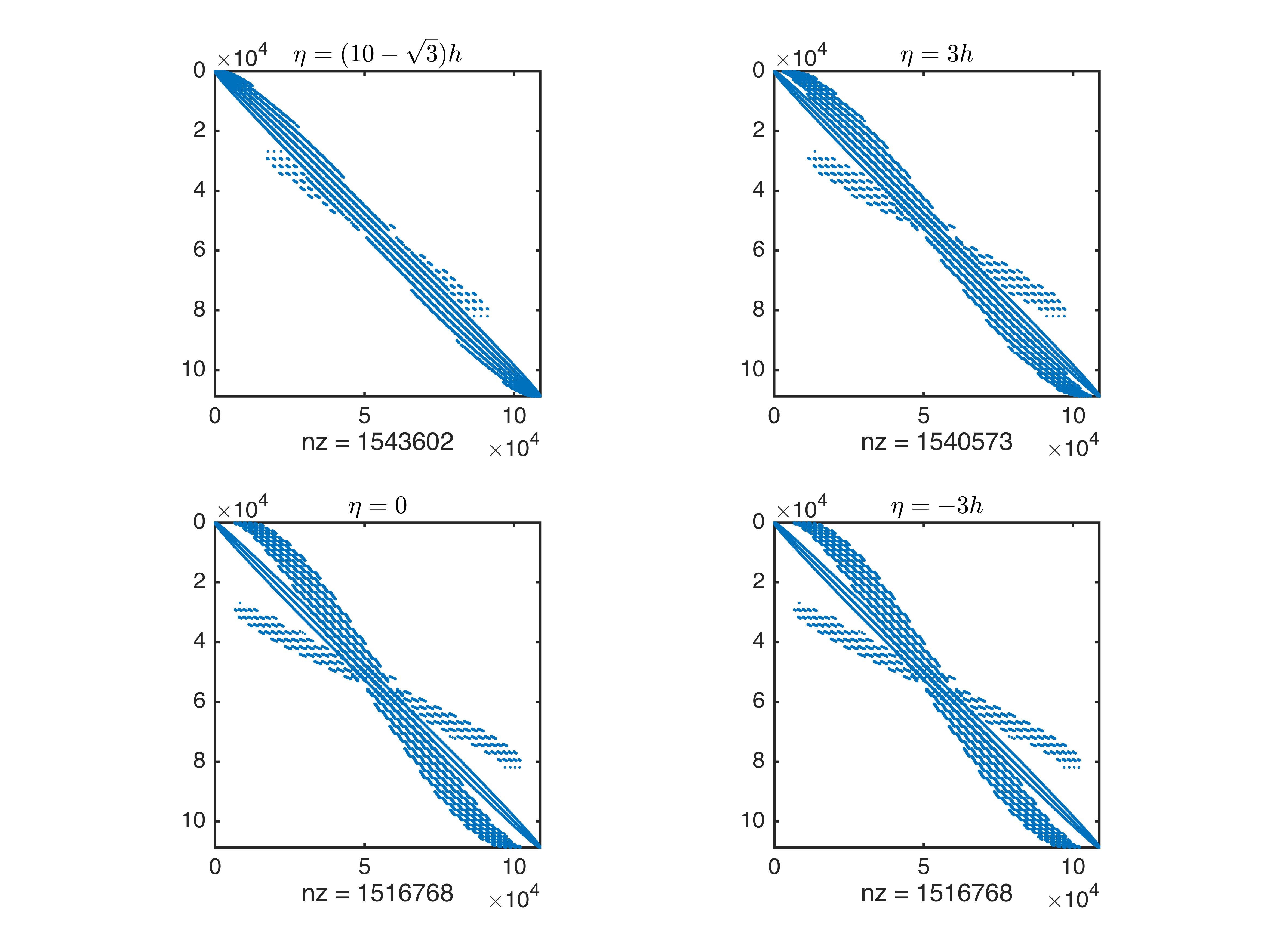
Figure 3: The structures of the matrices obtained from different $\eta=d(x)-\alpha$. The variable nz refers to the size of the matrices.

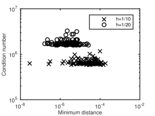
Figure 4: Distribution of minimum distances between inner nodes and the boundary of $T_{\epsilon}$ versus the condition numbers of reduced linear system among 100 times random perturbation on grid positions.

3.4.2 Eigenfunctions of the Laplace-Beltrami operator

On a circle in three dimensions

We consider the Laplace-Beltrami eigenvalue problem on a unit circle in $\mathbb{R}^{3}$ defined by

$$x(\theta)=\left[\begin{array}[]{l}x_{1}(\theta)\\ x_{2}(\theta)\\ x_{3}(\theta)\end{array}\right]=\left[\begin{array}[]{ccc}-\frac{7}{\sqrt{102}}&\frac{1}{\sqrt{2}}&\frac{1}{\sqrt{51}}\\ -\frac{7}{\sqrt{102}}&-\frac{1}{\sqrt{2}}&\frac{1}{\sqrt{51}}\\ \frac{2}{\sqrt{102}}&0&\frac{7}{\sqrt{51}}\end{array}\right]\left[\begin{array}[]{c}\cos\theta\\ \sin\theta\\ 0\end{array}\right],\,\,\,0\leq\theta<2\pi.$$ (3.25)

This circle is not symmetric in any way with respect to the underlying Cartesian grid, and we discretize this problem as if we are dealing with more general smooth curves without using the knowledge of the parametrization of the circle. Recall that the Laplace-Beltrami eigenvalue problem is to solve

$$\Delta_{\Gamma}u_{n}=\lambda_{n}u_{n}.$$ (3.26)

For simplicity, the kernel function is chosen to be constant. We choose two free convexification constants $\mu_{1}=\mu_{2}=\sigma^{-1}=1-d_{\Gamma}(p)\kappa(p)$, where $\kappa$ is the curvature of the parallel curve at point $p$. Hence $A=\sigma^{-1}I_{3}$ is a scalar tensor and the extended PDE on $T_{\epsilon}$ is

$$\sigma^{-1}\text{$\nabla$}\cdot(\sigma^{-1}\nabla v_{n})=\lambda v_{n}$$ (3.27)

In this case, $\sigma^{-1}=\sqrt{u_{1}^{2}+u_{2}^{2}},$ where $[u_{1},u_{2},u_{3}]^{T}=Rx$ and $R$ is the orthogonal matrix in (3.25). The first eigenvalue is 0 and simple and the corresponding eigenfunction is constant. The rest of the eigenvalues are $n^{2}$ for $n\in\mathbb{N}$, with multiplicity 2. The corresponding eigenfunctions are $\cos(n\theta+\phi)$ for any arbitrary phase shift $\phi$.

The numerical simulations are carried out on the grid nodes in $T_{\epsilon}\cap h\mathbb{Z}^{3}$ with $\epsilon=4h$, and $h$ is chosen to be $\frac{1}{10},\frac{1}{20},\frac{1}{40},\frac{1}{80},\frac{1}{160},\frac{1}{320}$. We discretize (3.27) by second order central difference and computed the eigenvalues of the discretized system as approximations of exact eigenvalues. The errors of eigenvalues are listed in Table 2. We can see the convergence rate is close to second-order. In Figure 5, we plot the eigenfunction corresponding to $\lambda=25$ on the equal distance surface $\Gamma_{2h}$ on the left hand side. The eigenfunction is close to constant on the normal cross section surface. If we projected the eigenfunction back to the unit circle, we can see it is close to $\cos 5\theta$ after suitable phase shift in right subfigure of Figure 5. The error of the eigenfunction in this case is of magnitude $10^{-5}$.

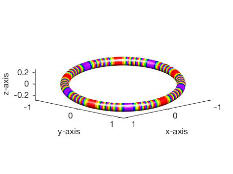
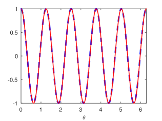
Figure 5: The eigenfunction of unit circle corresponding to $\lambda=25$. (Left) The eigenfunction on the torus surface that is the equal distant surface $\Gamma_{2h}$ with $h=1/20$. (Right) The eigenfunction with respect to the $\theta$ parameter on the curve. The blue dashed curve is numerical solution and the red solid curve is $\cos 5\theta$.

Table 2: The errors of the Laplace-Beltrami eigenvalue problem for a unit circle in $\mathbb{R}^{3}$.

$h^{-1}$	Error for $\lambda$ = 1	Error for $\lambda$ = 4	Error for $\lambda$ = 25	Error for $\lambda$ = 36
10	6.4982e-4	5.4573e-2	3.9316e-2	1.7026e-1
20	6.2345e-5	1.5447e-3	9.2460e-3	3.4550e-2
40	5.7136e-5	6.5797e-4	2.6530e-3	3.7635e-3
80	3.1412e-6	1.8924e-4	2.8500e-3	6.9070e-3
160	7.0887e-7	3.4274e-4	1.4435e-4	6.4697e-4
320	7.0887e-7	1.5974e-5	5.4665e-5	4.2973e-4
Order	1.8814	1.9144	1.8672	1.6997

On a torus in three dimensions

Let $\Gamma$ be the torus $(\sqrt{x^{2}+y^{2}}-0.7)^{2}+z^{2}=0.3^{2}$ in $\mathbb{R}^{3}$. Consider the Laplace-Beltrami eigenvalues $\lambda_{n}$ and eigenfunctions $\phi_{n}$ of $\Gamma$:

$$-\Delta_{\Gamma}\phi_{n}=\lambda_{n}\phi_{n}.$$

We compute the eigenvalues and eigenfunctions by solving the extended eigenvalue problems:

$$-J^{-1}\nabla\cdot(JA^{2}\nabla\psi_{n})=\lambda_{n}\psi_{n}\,\,\text{in}\,T_{\epsilon},\,\,\frac{\partial\psi_{n}}{\partial n}=0\,\,\text{on}\,\partial T_{\epsilon}.$$

In this numerical simulation, we use grid nodes in $T_{\epsilon}\cap h\mathbb{Z}^{3}$ with $\epsilon=4h$ and $h$ is chosen to be $\frac{1}{20}.$ We compute the discrete approximation of the differential operator of the extended equation. Then solve the eigenvalues and eigenvectors of the induced linear system. Figure 6 shows a computational result of an eigenfunction corresponding to the 6th eigenvalue $\lambda_{6}\simeq 6.51$ of the Laplace-Beltrami operator on the torus $\Gamma$.

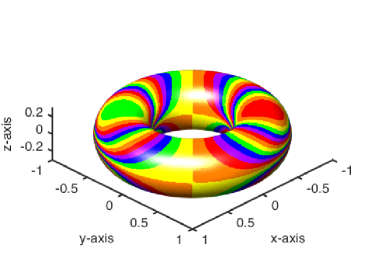
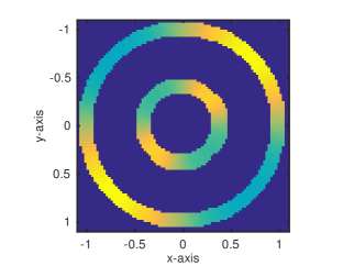
Figure 6: An eigenfunction of the Laplace-Beltrami operator on a torus. The results are computed by the proposed algorithm. (Left) The colormap used here reveals the structure of the eigenfunctions’ level lines. (Right) The $z=0$ section of the solution, indicating that the computed solution is indeed constant-along-normal.

3.4.3 Energy decay rates

Let $\Gamma$ be the ellipse with major axis equal to 4 and minor axis equal to 2 in $\mathbb{R}^{2}$. The angle between the major axis and positive $x-$axis is set to be $\frac{\pi}{5}$. See Figure 2 for illustration for the computational domain. The ellipse can be parametrized by

$$\left[\begin{array}[]{l}x(\theta)\\ y(\theta)\end{array}\right]=\left[\begin{array}[]{rr}\cos\frac{\pi}{5}&-\sin{\frac{\pi}{5}}\\ \sin\frac{\pi}{5}&\cos{\frac{\pi}{5}}\end{array}\right]\left[\begin{array}[]{r}2\cos\theta\\ \sin\theta\end{array}\right].$$

Notice that $\theta$ is not arc-length parameter and the arc-length function $s(\theta)=\int_{0}^{\theta}(3\sin^{2}\beta+1)\,d\beta$ is computed numerically. The energy function $I_{\Gamma}$ is given by $I_{\Gamma}(u)=\frac{1}{2}\int_{\Gamma}|\nabla_{\Gamma}u|^{2}\,dS=\frac{1}{2}\int_{\Gamma}u_{s}^{2}\,dS$. The gradient decent flow $u(t,s)$ of $I_{\Gamma}$ satisfies the heat equation

$$u_{t}=u_{ss}$$ (3.28)

on $\Gamma$. If we choose free variable $\mu=\sigma^{-1}$ and constant kernel function, the extended energy function $J_{T_{\epsilon}}$ of $I_{\Gamma}$ is

$$J_{T_{\epsilon}}(v)=\frac{1}{2}\int_{T_{\epsilon}}\sigma^{-1}|\nabla v|^{2}\>dz.$$ (3.29)

As discussed in Section 3.3, instead of solving

$$v_{t}=\nabla\cdot(\sigma^{-1}\nabla v),$$ (3.30)

the gradient flow of $J_{T_{\epsilon}}$ should be

$$v_{t}=\sigma^{-1}\nabla\cdot(\sigma^{-1}\nabla v).$$ (3.31)

In the numerical simulation, the initial data is set to be $u(s,0)=\sin(ks)$, where $k=\frac{2\pi}{L}$ and $L\simeq 9.6884$ is the total length of the ellipse $\Gamma$. The exact solution of (3.28) is $u(s,t)=e^{-k^{2}t}\sin(ks)$. We apply forward Euler in time and discretize the equation by using $\Delta x=\Delta y=h=\frac{1}{100}$ and $\Delta t=\frac{h^{2}}{10}$ with $\epsilon=3h$. We compare the $L_{\infty}$-error $\|v(s,\eta,t)-e^{-k^{2}t}\sin(ks))\|_{\infty,T_{\epsilon}}$ on $T_{\epsilon}$ and the energy decaying rate with the solutions obtained from (3.30), (3.31) numerically and from the closest point method [29]. We use the standard second order central difference scheme for $\nabla\cdot(\sigma^{-1}\nabla v)$ and bi-cubic interpolation in the boundary closure. The energy errors are integrated numerically using (2.11) with $\bar{L}=\frac{1}{2}|\nabla v|^{2}$and $K_{\epsilon}(d)=\frac{1}{2\epsilon}(1+\cos(\frac{d}{\epsilon}))\chi_{[-1,1]}(d)$ where $\chi_{[-1,1]}$ is the indicator function of $[-1,1]$. (2.11) is discretized be central differencing for $\nabla v$ and trapezoidal rule for the integral. For close point method, we use second order central difference scheme to compute Laplacian and bi-cubic interpolation for close point extension procedure. In computing the energy error in the solution of the closest point method, $|\nabla v|^{2}$ is replaced by the values on $\Gamma$, i.e. $|\nabla v(P_{\Gamma}x)|^{2}$. The results are shown in Figure 7. We can see the proposed method with correct decaying rate has smallest error in both $L_{\infty}$-norm and energy norm.

Next, we apply Crank-Nicolson time discretization for this example. The resulting matrices are inverted by the built-in GMRES scheme in Matlab to solve the linear system with tolerance $10^{-13}$. In Table 3, we report certain aspects of the computational results obtained with $h=\frac{1}{50},\frac{1}{100},\frac{1}{200},\frac{1}{400},\frac{1}{800,}\frac{1}{1600}$ , $\Delta t=\frac{h}{10}$ , $\epsilon=3h$; these include the condition numbers of the matrices $I-\frac{\Delta t}{2}Q_{h}$, where $Q_{h}$ corresponds to the centered differencing discretization of the spatial derivatives, the average of numbers of iterations and the $L_{\infty}$-errors $\|v(s,\eta,t)-e^{-k^{2}t}\sin(ks))\|_{\infty,T_{\epsilon}}$ on $T_{\epsilon}$ for $0\leq t\leq 2.$ The condition number scales like $O(\frac{1}{h})$ and the convergence rate is second-order as we expect.

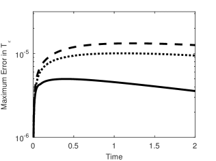
Figure 7: (Left) The $L_{\infty}$ -error on the narrowband $T_{\epsilon}$. (Right) The relative error of energy on the narrow band $T_{\epsilon}$. The solid curves are obtained by proposed method solving (3.31) and the dashed curves are with (3.30). The dotted curves are obtained by the closest point method.

Table 3: The performance of the proposed method with Crank-Nicolson method in time.

$h^{-1}$	Condition number	# of iterations	$L_{\infty}$-error	Order
50	23.94	8.2	1.4459e-5
100	45.00	9.7	3.5625e-6	2.0210
200	88.82	9.7	9.2893e-7	1.9393
400	176.70	12.6	2.2653e-7	2.0358
800	353.24	17.6	5.7933e-8	1.9673
1600	708.40	25.5	1.4441e-8	2.0042

3.4.4 Gradient flow of Allen-Cahn equation

Let $\Gamma$ be the ellipse given in Section 3.4.3. We consider the Modica-Mortola energy on $\Gamma$:

$$I_{\Gamma}(u)=\int_{\Gamma}\frac{\delta}{2}\|\nabla_{\Gamma}u\|^{2}+\frac{1}{4\delta}(1-u^{2})^{2}\,dS,\,\,\,0<\delta\ll 1,$$ (3.32)

and its gradient descent by the Allen-Cahn equation on $\Gamma$:

$$u_{t}=u_{ss}+\frac{1}{\delta^{2}}u(1-u^{2}).$$ (3.33)

The extended equation of (3.33) is simply

$$v_{t}=\sigma^{-1}\nabla\cdot(\sigma^{-1}\nabla v)+\frac{1}{\delta^{2}}v(1-v^{2}),\quad\text{on}\,\,T_{\epsilon},$$

with zero Neumann boundary condition. Since the Modica-Mortola energy is not strictly convex, the equation has non-unique minimizers and the minimizers depend on initial conditions. In this numerical experiment, we pick $\delta=0.03$. We use forward Euler in time and choose $h=\frac{1}{200}$, $\epsilon=0.3$ with $\Delta t=\frac{h^{2}}{10}$. The initial condition is set to be

$$v(x,0)=\sum_{j=11}^{13}\sin\left(\frac{2j\pi s^{2}}{L^{2}}\right),$$

where $L\simeq 9.6884$ is the total length of the ellipse $\Gamma$ and $s$ is the arc-length parameter on $\Gamma$. Since there is no analytical form for the exact solution, we use very fine grid (2000 equidistant points on $\Gamma$) and apply central difference scheme with forward Euler in time to discretize (3.33) directly as the reference solution. We compare our proposed method with a modified version of the closest point method (CPM). This modified CPM is not recommended in practice. We use this example to illustrate that CPMs have an internal time scale that is defined by the frequency of the “reinitialization” steps, and successful application of a CPM can depend on such internal time scale and its relation to the intrinsic time scale of the problem.

In the modified CPM, we solve

$$v_{t}=\Delta v(cp(x))+\frac{1}{\delta}v(1-v^{2})$$

by the standard central difference scheme for the Laplacian, and forward Euler method in time. Here $cp(x)=P_{\Gamma}x$ is the closest point function. Instead of reinitializing $v$ to be constant-along-normal after each time step (as in the original CPM), we reinitialize every $h/2$ time interval (every 1000 explicit Euler steps). The chosen time interval would be possible for a CPM that uses implicit time stepping, but as this example shows, this choice may not be appropriate. We refer the readers to [19] for the implicit closest point method, and emphasize that the real performance of an appropriately implemented implicit CPM may be different from what is presented in this example. The errors computed by two different methods are shown in Figure 8. The oscillation of the error computed by the modified CPM is due to the insufficient frequency of reinitialization compared to the small time scales in the dynamics. The large error near $t=1$ indicates the phase transition of the gradient descent is incorrect. In the right subfigure in Figure 8, we show the modified CPM solution at $t=0.9774975$, right before the reinitialization step. In the center subplot of the same Figure, we show the solution computed by the proposed method. The modified CPM solution, before the last reinitialization, is not constant-along-normal in the right top corner. One may see that in such region, reinitialization can either set $v$ to back to the right “phase” value or to the opposite phase value, depending of the developed pattern. Furthermore, since the transition time for Allen-Cahn is very short, if reinitialization in a CPM algorithm is not applied sufficiently frequently, the solution can lead to wrong gradient descent flow and possibly different steady state pattern.

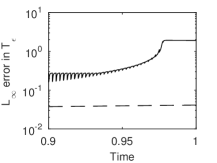
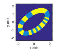
Figure 8: (Left) $L_{\infty}$-error in $T_{\epsilon}$ at different time step. The dashed line is obtained by the proposed method and the solid line is obtained by modified CPM. (Center) The snapshot of the solution by the proposed method at $t=$ 0.9774975. (Right) The snapshot of the solution by our modified CPM at the same time, before the last reinitialization step.

3.4.5 Minimization of $p$-Laplacian on a torus with constraint

Let $\Gamma$ be the torus $(\sqrt{x^{2}+y^{2}}-0.7)^{2}+z^{2}=0.3^{2}$ in $\mathbb{R}^{3}$. We can parametrize $\Gamma$ by $(x,y,z)=((0.7+0.3\cos\phi)\cos\theta,(0.7+0.3\cos\phi)\sin\theta,0.3\sin\phi),\theta,\phi\in[0,2\pi).$ Consider the energy function

$$I_{\Gamma}(u)=\frac{1}{p}\int_{\Gamma}|\nabla_{\Gamma}u|^{\,p}\,dS-\int_{\Gamma}f\,u\,dS.$$ (3.34)

with constraint

$$\|u\|_{2,\Gamma}=\int_{\Gamma}u^{2}\,dS=1.$$

We use the method proposed in Section 3.2 to solve the minimization problem of $I_{\Gamma}$ with the constraint. We solve the gradient flow

$$v_{t}=J^{-1}\nabla\cdot(|\,A\nabla u\,|^{p-2}JA^{2}\nabla v)+\overline{f}+\lambda(t)v,$$

on the narrowband $T_{\epsilon}$ of $\Gamma$ and the Lagrange multiplier is chosen to be

$$\lambda(t)=\frac{\int_{T_{\epsilon}}|\,A\nabla v\,|^{p}JdS-\int_{T_{\epsilon}}\overline{f}\,v\,JdS}{\int_{\Gamma}v^{2}J\,dS}.$$

In the following examples, we choose the parameter $\mu$ to be $1$ and the kernel $K$ to be constant. The numerical simulations are carried out on the grid nodes in $T_{\epsilon}\cap h\mathbb{Z}^{3}$ with $\epsilon=4h$, and $h$ is chosen to be $\frac{1}{25},\frac{1}{50}.$

We first choose $p=3$, $f=1$. In this case, the minimizer is $u=\frac{1}{c}$ with $c=\sqrt{\frac{84}{100}}\pi$, the square root of surface area of $\Gamma$ and the minimal energy $I_{\Gamma}$ is $-c$. We use two different initial conditions $u_{1}(\theta,\phi)=\frac{2}{c}\sin\theta\cos\phi$ and $u_{2}(\theta,\phi)=\frac{2}{c}\cos\theta\sin\phi$, $\theta,\phi\in[0,2\pi)$ on $\Gamma$ and extend them constant-along-normal to get initial condition for extended equations. For time discretization, we use forward Euler with $\Delta t=\frac{h^{2}}{10}$ to compute the solution until $\|v(t+\Delta t)-v(t)\|_{T_{\epsilon},\infty}<10^{-7}.$ The total energy error $J_{T_{\epsilon}}(v(t))+c$ and $L_{2}-$norm error $|\frac{1}{2\epsilon}\int_{T_{\epsilon}}v^{2}(t)J\,dS-1|$ are shown in Figure 9. We can see the total energy converges to the exact energy value $-c$ for both choices of initial conditions. From the right subfigure in Figure 9, we see that the $L_{2}-$norm is almost conserved by the proposed method and converges to $0$ as $h$ tends to $0$.

For a nontrivial numerical example, we choose $p=3$, and $f=\cos(\theta+\phi)\sin(\phi)$. For this problem, we do not have analytical form for the minimizer. The total energy $J_{T_{\epsilon}}(v(t))$ and $L_{2}-$norm error $|\frac{1}{2\epsilon}\int_{T_{\epsilon}}v^{2}(t)J\,dS-1|$ are shown in Figure 10. Again, we can see energy decays to some steady state for both initial conditions and the $L_{2}-$norm is almost conserved by the proposed method.

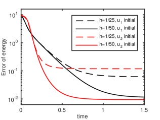
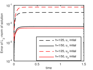
Figure 9: (Left) The total energy error $J_{T_{\epsilon}}[v]+c.$ (Right) The error of $|\|v\|_{2,\Gamma}-1|$. We use $h=\frac{1}{25}$ and $h=\frac{1}{50}$ with two different initial condition $u_{1}$ and $u_{2}$. The dashed and solid curves are for $h=\frac{1}{25}$ and $h=\frac{1}{50}$ respectively. The black and red curves are using initial condition $u_{1}$ and $u_{2}$ respectively.

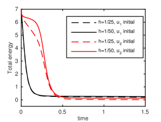
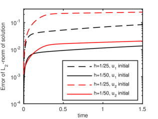
Figure 10: (Left) The total energy $J_{T_{\epsilon}}[v].$ (Right) The error of $|\|v\|_{2,\Gamma}-1|$. We use $h=\frac{1}{25}$ and $h=\frac{1}{50}$ with two different initial condition $u_{1}$ and $u_{2}$. The dashed and solid curves are for $h=\frac{1}{25}$ and $h=\frac{1}{50}$ respectively. The black and red curves are using initial condition $u_{1}$ and $u_{2}$ respectively.

4 Least action principles

We shall consider the model least action principle defined by

$$I_{\Gamma}[u]:=\int_{t_{1}}^{t_{2}}\int_{\Gamma}\left[\left(\frac{\partial u}{\partial t}\right)^{2}-|\nabla_{\Gamma}u|^{2}\right]dS(x)\,dt,$$

which consists of the difference between the kinetic energy and the potential energy. Taking the variational derivative, the resulting Euler-Lagrange equation is an analogy of the usual second order wave equation, but defined on $\Gamma$.

Correspondingly, we shall study the extensions of $I_{\Gamma}$ in the following form

$$\tilde{I}_{T_{\epsilon}}[v]:=\int_{t_{1}}^{t_{2}}\int_{T_{\epsilon}}\left[\left(\frac{\partial v}{\partial t}\right)^{2}-|A(z;\mu)\nabla u|^{2}\right]K_{\epsilon}(d_{\Gamma}(z))J(z)dz\,dt.$$ (4.35)

Recall that $A(z;\mu):=\left(\sigma_{1}^{-1}\mathbf{t}_{1}\otimes\mathbf{t}_{1}+\sigma_{2}^{-1}\mathbf{t}_{2}\otimes\mathbf{t}_{2}+\mu\mathbf{n}\otimes\mathbf{n}\right).$ Hence the essential questions are about the well-posedness of the extended problem, with or without the additional component $(\frac{\partial u}{\partial n})^{2}$ in the potential energy of the system, and stability of the constant-along-normal solutions.

Notice that unlike elliptic equations, the zero Neumann boundary condition is not the natural boundary condition for the variational problem involving energy $\tilde{I}_{T_{\epsilon}}$ defined in (4.35). The natural boundary condition is the radiation boundary conditions (add citation). However, the constant-along-normal solutions usually do not satisfy the radiation boundary conditions.

4.1 Study of a model problem

Consider $\Gamma$ to be the unit interval on the $x$-axis with periodic boundary conditions at $x=0$ and $1$, and $T_{\epsilon}=[0,1)\times(-\epsilon,\epsilon).$ Thus the Euler-Lagrange equation of $\tilde{I}_{T_{\epsilon}}$ satisfies

$$v_{tt}=v_{xx}+\mu v_{yy},\,\,\,(\mu\geq 0)$$ (4.36)

We look for periodic solutions

$$v(x+1,y,t)=v(x,y,t)$$ (4.37)

satisfying the constant-along-normal initial conditions

$$\begin{cases}v(x,y,0)=v_{0}(x),\\ v_{t}(x,y,0)=v_{t,0}(x),\end{cases}$$ (4.38)

and the Neumann boundary condition

$$\frac{\partial v}{\partial y}(x,\pm\epsilon,t)=0.$$ (4.39)

For $\mu=0,$ we have a family of one-dimensional wave equation, coupled only through the initial conditions. It is obvious that for $\mu\geq 0,$ the initial-boundary-value problem (4.36)-(4.39) is well-posed and stable. Furthermore, it is easy to show that the solutions starting with the initial conditions (4.38) will stay constant-along-normal, i.e. $v_{y}(x,y,t)=0$ for all time.

In this case, the natural boundary condition is $v_{t}\pm v_{y}=0$ on $y=\pm\epsilon$. For this model problem, the constant-along-normal solutions are superposition of plane waves of the form $e^{i(kx\pm kt)}$. Obviously, the planes wave solutions do not satisfy the natural boundary conditions unless they are constants.

In the following, we shall look into the effect of perturbations that might be introduced by discretization.

4.1.1 Perturbation in the initial conditions

We consider the solutions of the form

$$u(x,y,t)=f(x+t)+g(x-t)+C(y,t),\,\,\,C(y,0)=C_{t}(y,0)=0.$$

For $\mu\geq 0$, $C(y,t)$ can only be zero due to the special form of the initial conditions. Now, suppose that the initial condition is not exactly constant along the normals of $\Gamma$, the equation with $\mu=0$ will admit solutions that grow linearly in time.

To see this, consider $\frac{\partial v}{\partial y}(x,y,0)=0$ and

$$\frac{\partial}{\partial y}v_{t}(x,y,0)=-\delta\sin\frac{\pi y}{\epsilon}\,\,\,\text{for some }\delta\in\mathbb{R}.$$

This means that the initial condition of $v_{t}$ has a sinusoidal perturbation satisfying the Neumann boundary condition. Then $C(y,t)=\frac{\delta\epsilon}{\pi}\cos\frac{\pi y}{\epsilon}\cdot t.$ Computationally, if both $\delta$ and $\epsilon$ are of order $h$, with $h$ the grid spacing, this initial perturbation will introduce only $O(t\cdot h^{2})$ difference in the solutions.

With $\mu>0,$ the perturbation in the initial conditions will result in modes that propagate towards the boundaries and then be reflected back into the domain. Nevertheless, since the total energy is conserved, we expect that such perturbation will stay controlled.

4.1.2 Perturbation in the boundary conditions

In general, numerical discretization of the Neumann boundary condition (4.39) will inevitably introduce some tangential perturbations that could be modeled by:

$$\frac{\partial v}{\partial y}(x,\epsilon,t) =\alpha\frac{\partial^{k}v}{\partial x^{k}}(x,\epsilon,t),\,\,\,\alpha\in\mathbb{R},k\geq 1,$$ (4.40)

and

$$\frac{\partial v}{\partial y}(x,-\epsilon,t)=0.$$ (4.41)

Consider the following two 4th order boundary closures for the grid nodes $(ih,(N+1)h)$:

$$u_{i,N+1}:=\frac{2}{3}(u_{i-1,N-1}+u_{i+1,N-1})-\frac{1}{6}(u_{i-2,N-1}+u_{i+2,N-1}),$$

leading to

$$v_{y}\approx\frac{1}{6}h^{4}u_{xxxx},$$

and

$$u_{i,N+1}:=\frac{1}{4}u_{i-1,N-1}+\frac{3}{2}u_{i+1,N-1}-u_{i+2,N-1}+\frac{1}{4}u_{i+3,N-1},$$

leading to a perturbation to the zero Neumann condition with the leading order term of a different sign:

$$v_{y}\approx-\frac{1}{4}h^{4}u_{xxxx}.$$

A natural question is whether such perturbation will render the resulting initial-boundary-value problem ill-posed? We follow closely the theory developed in [13], and particularly in [16]. We use Laplace transform in time and Fourier transform in the $x$-variable to study the well-posedness of the perturbed problem (4.36)-(4.38) and (4.40)-(4.41). Due to linearity of the problem, we may analyze by a single mode:

$$\hat{v}(\omega,y,s)=e^{st}e^{i\omega x}\phi(y).$$ (4.42)

Suppose that there exists $s_{0}\in\mathbb{C}$ with $\text{Re }s_{0}>0$ and $\omega_{0}\in\mathbb{Z}$ such that $\hat{v}$ solves (4.36)-(4.38) and (4.40)-(4.41).

We first remark that even with constant-along-normal initial conditions (4.38), $v_{y}$ will not remain $0$ in time, due to the perturbed boundary condition (4.40), unless $v$ is a constant. Therefore, we cannot just consider $\phi(y)$ being a constant. Plugging (4.42) into the equation, we obtain

$$s^{2}\phi=-\omega^{2}\phi+\mu\phi_{yy}.$$

Without loss of generality we analyze $\mu=1$ for the case $\mu>0$. We have the eigenvalue problem

$$\phi_{yy}=(s^{2}+\omega^{2})\phi,$$ (4.43)

with the boundary conditions

$$\phi_{y}(\epsilon)=\alpha(i\omega)^{k}\phi(\epsilon),$$ (4.44)

and

$$\phi_{y}(-\epsilon)=0.$$

$$\phi(y)=c_{1}e^{\kappa y}+c_{2}e^{-\kappa y},\,\,\,\kappa:=(s^{2}+\omega^{2})^{\frac{1}{2}},$$

where the square root is taken on the complex plane with the branch $-\pi<\arg z\leq\pi.$ Solutions with $\kappa=0$ are stable, so we will not discuss such a case. If $\kappa\neq 0$, from the boundary conditions, we have

$$c_{1}=c_{2}e^{2\kappa\epsilon},$$

and

$$(\kappa-\alpha(i\omega)^{k})e^{4\kappa\epsilon}=(\kappa+\alpha(i\omega)^{k}).$$ (4.45)

$k$ is an even positive integer.

In this case, (4.45) is equivalent to $\kappa\tanh(2\kappa\epsilon)=\tilde{\alpha}\omega^{k}$, where $\tilde{\alpha}=\alpha i^{k}$. This equation admits only pure imaginary solution $\kappa$ if $\tilde{\alpha}\leq 0$; and it has at least one real solution $\kappa$ if $\tilde{\alpha}>0$. Thus we conclude that $s=(\kappa^{2}-\omega^{2})^{\frac{1}{2}}$ is a pure imaginary number if $\tilde{\alpha}<0$, and in this case the equation is stable. On the other hand, we have $s=(\kappa^{2}-\omega^{2})^{\frac{1}{2}}>0$ if $\tilde{\alpha}>0$. Therefore the equation is unstable when $\tilde{\alpha}>0$.

$k$ is an odd positive integer.

In this case, (4.45) is equivalent to

$$\frac{\tau+bi}{\tau-bi}=e^{\tau},$$ (4.46)

where $\tau=4\epsilon\kappa,b=4\epsilon\alpha i^{k-1}\omega^{k}$. Suppose $\tau=u+vi$, then by equating the modulus in both sides of (4.46) we have

$$\frac{u^{2}+(v+b)^{2}}{u^{2}+(v-b)^{2}}=e^{2u}.$$

Hence we have $v=f(u)=\frac{b(e^{2u}+1)\pm\sqrt{4b^{2}e^{2u}-u^{2}(e^{2u}-1)^{2}}}{e^{2u}-1}$ and $v$ is real if $u\sinh u\leq|b|$. Notice that $\omega=2n\pi$ can be arbitrary large so can $|b|$. To show (4.46) admits a solution, we check that

$$\frac{u+(v+b)i}{u+(v-b)i}=e^{2u}e^{vi}\iff\frac{u+(f(u)+b)i}{u+(f(u)-b)i}=e^{2u}e^{f(u)i}.$$

We only need to show there exists $u$ such that the arguments of both sides in the above equation are equal. With out loss of generality, we assume $b>0$. Let $u^{*}>0$ satisfies $u^{*}\sinh u^{*}=b$. Then $f(u^{*})=u^{*}\cosh(u^{*})$ and $arg(\frac{u^{*}+(f(u^{*})+b)i}{u^{*}+(f(u^{*})-b)i})\rightarrow arg(e^{u^{*}}i)=\frac{\pi}{2}$ as $|b|\rightarrow\infty.$ Therefore for large enough $b$ and $u$ close to $u^{*}$ enough, $arg(\frac{u+(f(u)+b)i}{u+(f(u)-b)i})\simeq\frac{\pi}{2}$. Since $f(0)=0$ and $f(u)$ is increasing, by continuity of $f(u)$, for large enough $\omega,$ there always exists $\tau=u+f(u)i$ that satisfies (4.46). Therefore $s=\sqrt{\frac{\tau^{2}}{16\epsilon^{2}}-\omega^{2}}$ with positive real part satisfies the eigenvalue problem. This means that the perturbed boundary condition admits solutions that exponentially increase in time and have boundary layers of near $\partial T_{\epsilon}$.

4.1.3 General positive values of $\mu$.

$s$ is replaced by $s/\sqrt{\mu}$ in the analysis above, and the unstable modes become

$$\hat{v}(x,y,t)\sim e^{\mu st}e^{i\omega x}(c_{1}e^{\mu\kappa y}+c_{2}e^{-\mu\kappa y}).$$

We see that with small values of $\mu$, the instability can be controlled.

For $\mu=0,$ we have

$$(s^{2}+\omega^{2})\phi(y)=0.$$

Non-trivial solutions requires that $s=\pm i\omega$. We then look for $\phi(y)$ which satisfies

$$\phi_{y}(\epsilon)=\alpha(i\omega)^{k}\phi(\epsilon),\,\,\,\phi_{y}(-\epsilon)=0.$$

The set of $C^{2}$ functions which satisfy the two conditions are not bounded. Thus we have to estimate the solution from the initial conditions.

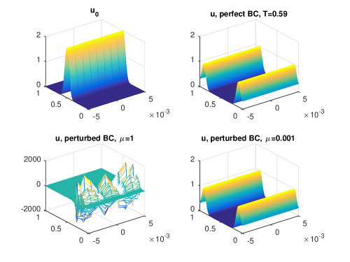
Figure 11: Unstable wave solutions by a 3rd order boundary closure, and stabilization by using smaller $\mu$.

Figure 11 demonstrates the instability analyzed above as well as the simple stabilization by using a small $\mu.$ Figure 12 demonstrates a numerical simulation using these two boundary closures with different values of $\mu$.

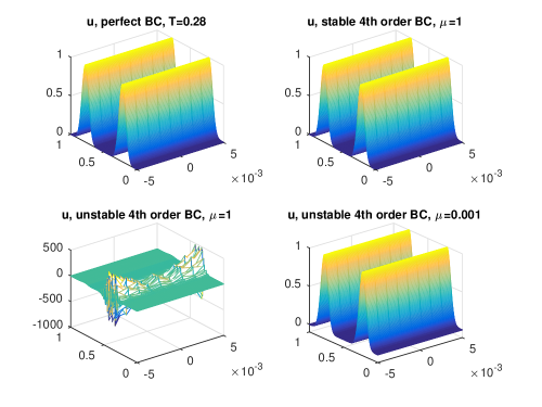
Figure 12: Wave solutions with stable and unstable 4th order boundary closure, and stabilization by using smaller $\mu$.

4.2 Perturbed boundary condition and stability

The mode analysis above shows that the instability exists in the normal derivatives of the solutions. We may explain the onset of instability as follows: waves are being bounced back and forth in between the two boundaries of $T_{\epsilon}$, and each time reflection takes place, the solution may loss some regularity, and after a few reflections, the accumulated instability dominates the computed system. In fact, the loss of regularity can be read off from the perturbed boundary conditions: the normal derivative of the reflected solution is set to the derivative of the part of the solution that caused the reflection. We can also understand at a heuristic level that without dissipation, such instability is hard to avoid for more general domains with curved boundaries (where as for dissipative systems, such problem is less prone to happen).

We also see this mechanism directly from the model equation and conditions satisfied by $w=v_{y}$:

$$w_{tt}=w_{xx}+\mu w_{yy},\,\,\,(\mu\geq 0),$$ (4.47)

satisfying the periodic condition in $x$:

$$w(x+1,y,t)=w(x,y,t),$$ (4.48)

the Neumann boundary conditions

$$w(x,\epsilon,t) =\alpha\frac{\partial^{k}v}{\partial x^{k}}(x,\epsilon,t),$$ (4.49)

$$w(x,-\epsilon,t) =0,$$ (4.50)

and the constant-along-normal initial conditions for $v$:

$$\begin{cases}w(x,y,0)=0,\\ w_{t}(x,y,0)=0.\end{cases}$$ (4.51)

We first see that by reducing the size of $\mu$, we delay the propagation of the boundary perturbation into the domain. Due to the special form of the initial conditions, we expect that the instability reflected in the discretized system comes out after constant multiply of discrete time steps.

For general curved boundaries, we cannot rely on diminishing the size of $\mu$ to prolong the onset of the instability. Suppose that we set $\mu=0$ in the equation for $v$, and analytically, with the constant-along-normal initial data, the solution will constants of wave that propagates only tangentially to $\Gamma_{\eta}.$ However, in the discretized system, a wave that is tangential to the boundary at a grid node at time $t^{n}$ will not be exactly tangential when it arrives at a neighboring grid node at a later time. And there, a reflection of this wave will take place. The following numerical simulations verify the discussion above.

Example 4.1.

(Stability against perturbation in the initial conditions) Let $\Gamma$ be the ellipse with major axis equal to 4 and minor axis equal to 2 in $\mathbb{R}^{2}$ as described in Section 3.4.3. We consider the wave equation on $\Gamma:$ $u_{tt}=u_{ss}$, where $s$ is the arc length of $\Gamma$ and the exact solution is given by $u(s,t)=\sin(\frac{2\pi(s-t)}{L})$. The extended wave equation on $T_{\epsilon}$ is

$$v_{tt}=\sigma^{-1}\nabla(A(\sigma;\mu)\nabla v),$$ (4.52)

where $A(\sigma;\mu)=\sigma^{-1}{\bf t}\otimes{\bf t}+\mu{\bf n}\otimes{\bf n}$. We use leapfrog scheme in time and second order central difference scheme in space to discretize (4.52). See Appendix for detail of discretization. The boundary nodes are interpolated by bi-cubic interpolating polynomials. To see the effect of being constant-along-normal or not, we perturb the initial condition in the numerical simulation. The initial condition is given by

$$v(s,\eta,0)=(C+(1-C)\cos\frac{\pi\eta}{2\epsilon})\sin(\frac{2\pi s}{L}),v(s,\eta,\Delta t)=(C+(1-C)\cos\frac{\pi\eta}{2\epsilon})\sin(\frac{2\pi(s-\Delta t)}{L}).$$

The parameter $C$ is to control the intensity of the perturbed initial condition away from being constant-along-normal. When $C=1$, the initial data is constant-along-normal; The smaller $C$ the bigger variance along the normal direction. We use $h=\frac{1}{100},\frac{1}{200},\frac{1}{400}$, $\epsilon=3h,6h,0.1$, $C=1,0.9,0.8$ and $\Delta t=\frac{h}{10}$ to test how fast the instability exhibits. We compute the solution until time step $t_{blow}$ such that $\|v(t_{blow})\|_{T_{\epsilon},\infty}>1.5$ and use $t_{blow}$ as the indicator for instability. From Figure 13, we see that it makes sense to use a smaller $\mu$ so that the instability occurs later. However, having it too small or zero will not be beneficial. Numerical evidence shows that the best choice of $\mu$ is about size of $h$. We also notice that the wider of bandwidth $\epsilon$ can delay the blowup time for some cases but not efficiently. Being far away from constant-along-normal produces the instability in a very short time. The smaller grid size $h$ causes the smaller blowup time. Numerically it shows that the blowup time is of order $O(h).$ In other words, the instability accumulates in each iteration independent of grid size $h$.

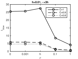
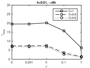
Figure 13: Blowup time $t_{blow}$ for different grid size $h$ and bandwidth $\epsilon$. The larger perturbation in normal direction produces the instability faster. The smaller $\mu$ can delay the onset of instability. The blowup time $t_{blow}$ scales like $O(h)$.

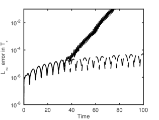
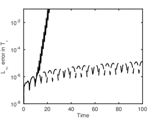
Figure 14: Reinitialization strategy to stabilize the wave equation. We use $h=1/200$ in the left figure and $h=1/400$ in the right figure. The dashed and solid curves are obtained by reinitializing per 0.1 and 1 time step.

4.3 Stabilization strategies and examples

4.3.1 Reinitialization

For general initial data, the unstable modes will dominate the solution also instantaneously. However, for constant-along-normal initial data considered in our particular problems, particularly with smaller values of $\mu$, the unstable modes seem to take longer time to become dominant.

Therefore, we propose to stabilize the computations by reinitializing the computed solutions periodically. By reinitializing a function $f_{0}$, we mean to create a new function $f$, which is the constant-along-normal extension of $f_{0}|_{\Gamma}$. Such reinitialization can be done easily by applying the boundary closure strategy to every inner node, projecting them onto $\Gamma$. It can also be done easily by solving the constant-extension PDE, used in the level set method, see e.g. [25, 5]. In a “Closest Point Method”, this step is a mandatory part of every discrete time step.

To demonstrate the strategy, we use the same setting as in Example 4.1. We reinitialize the solution per 0.1 and 1 time unit (or equivalently per $h^{-1}$ and $10h^{-1}$ discrete time steps). In this experiments, we test for $h=\frac{1}{200},\frac{1}{400}$ and compare the $L_{\infty}$-error $\|v(s,\eta,t)-\sin(\frac{2\pi(s-t)}{L})\|_{\infty,T_{\epsilon}}$ . The results are shown in Figure 14. The solid curves are obtained by reinitializing per 0.1 time unit and the dashed curve are obtained by reinitializing per 1 time unit. We see that the solutions is stable for much longer time after reinitialization. However, if the reinitialization is not frequently enough, the instability accumulates after certain iterations and the solution is unstable.

4.3.2 “Dissipative” regularization

Another way to stabilize the solution is to follow and adapt the idea proposed in [16]. Consider our model problem in the strip:

$$v_{t}=v_{xx}+\mu v_{yy}-\alpha v_{txxxx},\>\,\forall(x,y)\in[0,1)\times(-\epsilon,\epsilon),\,\alpha>0,$$

with the perturbed boundary condition

$$v_{y}(x,-\epsilon,t)=0,\,v_{y}(x,\epsilon,t)=av_{xxxx}.$$

In the same fashion as employed earlier in this section, it is proven in Section 6 and Appendix B of [16], that with this regularization and a suitable $\alpha$, the resulting initial boundary value problem is well-posed.

For general setups, the regularization will correspond to higher order tangential derivatives of the solution, and is not very convenient to discretize. Therefore, we propose to add to the equation for $v$ an isotropic version of this regularization that involve only the similar partial derivatives along the coordinate directions. This means, in two dimensions, we shall modify the PDE by

$$v_{tt}=\sigma^{-1}\nabla\cdot(\sigma^{-1}\nabla v)-\alpha h^{3}(v_{txxxx}+v_{tyyyy})$$

and discretize it on Cartesian grids by

$$\frac{v_{i,j}^{n+1}-2v_{i,j}^{n}+v_{i,j}^{n-1}}{\Delta t^{2}}=\mathcal{A}_{i,j}v_{ij}^{n}-\alpha h^{3}(D_{+}^{x}D_{-}^{x})^{2}\left(\frac{v_{i,j}^{n}-v_{i,j}^{n-1}}{\Delta t}\right)-\alpha h^{3}(D_{+}^{y}D_{-}^{y})^{2}\left(\frac{v_{i,j}^{n}-v_{i,j}^{n-1}}{\Delta t}\right),$$

where $\alpha\leq\frac{c}{4}$, $c$ is the maximum wave speed and $\mathcal{A}_{i,j}v_{i,j}^{n}$ is the discretization of $\sigma^{-1}\nabla\cdot(\sigma^{-1}\nabla v)$.

To demonstrate the effect of stabilization, we use the same setting in Example 4.1. We add the stabilization terms and use $\alpha=\frac{1}{5}$ with $h=\frac{1}{100},\frac{1}{200},\frac{1}{400}$ and $\Delta t=\frac{h}{10}$. We compare the $L_{\infty}$-error $\|v(s,\eta,t)-\sin(\frac{2\pi(s-t)}{L})\|_{\infty,T_{\epsilon}}$ for different $\mu$ and the results are shown in Figure 15. Notice that, to compute $(D_{+}^{x}D_{-}^{x})^{2}$ and $(D_{+}^{y}D_{-}^{y})^{2}$ terms, we need more ghost nodes. We see the solution becomes stable for very long time $T\geq 60$. Moreover, the solution has the same magnitude $L_{\infty}$-error as the solution without stabilization terms in the short time. This means the stabilization does not compromise the accuracy but regain the stability for $\mathcal{O}(1)$ time step. Also the results show the importance to choose free parameter $\mu$ close to $\mathcal{O}(h)$. The solution has smaller error for smaller $\mu$.

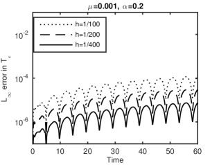
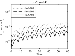
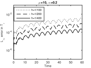
Figure 15: The $L_{\infty}$-error of solutions for wave equations with stabilization terms.

5 Summary

In this paper, we derive extensions of a class of integro-differential operators defined on smooth closed manifolds. The extended operators are defined for functions defined on thin narrowbands around the manifolds. The main objective is to provide a formulation that allows for construction of simple and accurate numerical algorithms that solve for the Euler-Lagrange equations of the functionals defined by these integro-differential operators, especially for the applications in which the manifolds are defined by the distance function or closest point mapping to the manifolds.

What distinguishes this work from other existing level set or closest point methods is that fact that our formulation solves the Euler-Lagrange equations of the extended, volumetric integrals, with the corresponding natural boundary condition on the boundaries of the narrowbands. We investigate how the extensions can be made to guarantee a strict equivalence between the solutions of the extended and the original problems. As a result, eigenvalue problems involving the Laplace-Beltrami operators can easily be computed. Together with our mathematical formulation, we propose a simple boundary closure procedure that can be adapted to a variety of numerical methods. We further study the stability and well-posedness of a few model (initial)-boundary-value problems. We discovered that hyperbolic problems require additional stabilization to curb the effect of unstable mode originated from the approximation of boundary conditions. We propose two strategies to stabilize the numerical algorithms. One involves adding higher order “dissipative” terms to the PDEs, and the other one involves “reinitializing” the solutions of the PDEs periodically. The reinitialization is similar to a required step in the closest point method. However, due to the special form of the initial conditions and the equations, the stabilization step is required only infrequently.

We remark that the proposed formulation is not limited to implementation using Cartesian grids. It is also convenient for design of finite element methods on non-body fitted mesh. Furthermore, the proposed formulation, which considers minimization of the variational principles instead of tackling directly the Euler-Lagrange equations, allows for the possibility of applying numerical optimization algorithms to the discretized variational principles. A potential advantage of such strategy include better preservation of invariances of the systems, see for example the variational integrator [20], and the flexibility in dealing with nonlinear degenerate systems such as the total variations of a function on surfaces [4]. This direction will be pursued in a future work.

Appendix A Appendix

A.1 Extension of surface gradient and surface divergence in $\mathcal{\mathbb{R}}^{3}$

Let $\Omega\subset\mathbb{R}^{3}$ be a bounded open set with $C^{2}$ boundary $\Gamma=\partial\Omega$. For simplicity, we assume there exists a signed-distance function $d:\mathbb{R}^{3}\rightarrow\mathbb{R}$ such that $\Gamma$ is the zero-level set of $d$. Without loss of generality, we also assume that $d<0$ on the interior of $\Gamma$ and $d>0$ on the exterior. The normal vector ${\bf n}(x)=\nabla d(x)$ is the unit outer normal vector field of $\Gamma$ and the projection $\Pi=I-{\bf n}\otimes{\bf n}$ which maps vectors in $\mathbb{R}^{3}$ onto the tangent space of $\Gamma$ at $x$. For any smooth function $u$ defined on $\Gamma$, the tangent gradient of $u$ is defined by

$$\nabla_{\Gamma}u(x)=\Pi\nabla\tilde{{u}}(x),\quad\forall x\in\Gamma,$$

where $\tilde{{u}}$ is any $C^{1}$ extension of $u(x)$ in a neighborhood of $x$. For any vector field $F$ defined on $\Gamma$, the surface divergence $\nabla_{\Gamma}\cdot F$ is defined analogously. Recall that $\eta$-level set of $d$ is $\Gamma_{\eta}=\{x\in\mathbb{R}^{3}\,|\,d(x)=\eta\}$ and $T_{\epsilon}=\cup_{|\eta|<\epsilon}\Gamma_{\eta}$ is the narrowband of $\Gamma$. The following theorem relates normal extension of the surface gradient and divergence to the Eulerian gradient and divergence of normal-extended function.

Theorem A.1.

Suppose $u$ is a smooth function defined on $\Gamma$. Let $P_{\Gamma}$ denote the closest point mapping and $\overline{u}$ denote the constant-along-normal extension of u in $T_{\epsilon}$. Then for any $z\in T_{\epsilon}$ , we have

$$\overline{\nabla_{\Gamma}u(z)}\equiv\nabla_{\Gamma}u\circ P_{\Gamma}(z)=A(z;\mu)\nabla\overline{u}(z),$$ (A.53)

where $A(z;\mu)=A_{0}(z)+\mu A_{1}(z),$

$$A_{0}(z):= \sigma_{1}^{-1}\mathbf{t}_{1}\otimes\mathbf{t}_{1}+\sigma_{2}^{-1}\mathbf{t}_{2}\otimes\mathbf{t}_{2},$$

$$A_{1}(z):= \mathbf{n}\otimes\mathbf{n},$$

where $\mathbf{t}_{1}$, $\mathbf{t}_{2}$ are the two orthonormal tangent vectors corresponding to the directions that yield the principle curvatures of $\Gamma$, $\mathbf{n}$ is the unit normal vector of $\Gamma$, $\sigma_{1}$ and $\sigma_{2}$ are two largest singular values of $DP_{\Gamma}$ and $\mu$ is any real number.

Suppose $F$ is a smooth vector field defined on $\Gamma$. Let $\overline{F}$ denote its constant-along-normal extension in $T_{\epsilon}$. Then for any $z\in T_{\epsilon}$ , we have

$$\overline{\nabla_{\Gamma}\cdot F(z)}\equiv(\nabla_{\Gamma}\cdot F)\circ P_{\Gamma}(z)=\sigma_{1}^{-1}\sigma_{2}^{-1}\nabla\cdot(B(z;\mu)\overline{F}(z))=J^{-1}\nabla\cdot(B(z;\mu)\overline{F}(z)),$$ (A.54)

where $B(z;\nu)=B_{0}(z)+\nu B_{1}(z),$

$$B_{0}(z):= \sigma_{2}\mathbf{t}_{1}\otimes\mathbf{t}_{1}+\sigma_{1}\mathbf{t}_{2}\otimes\mathbf{t}_{2}=\sigma_{1}\sigma_{2}A_{0}(z)=JA_{0}(z),$$

$$B_{1}(z):= \mathbf{n}\otimes\mathbf{n},$$

where $\nu$ is any real number. In particular, if we choose $\nu=J\mu$, then $B(z;\nu)=JA(z;\mu)$.

Proof.

Let $(s_{1},s_{2})$ be a local coordinate system for $\Gamma$ such that ${\bf t}_{1}=\frac{{\partial\Gamma(s_{1,}s_{2})}}{\partial s_{1}}$ and ${\bf t}_{2}=\frac{{\partial\Gamma(s_{1,}s_{2})}}{\partial s_{2}}$ are orthogonal unit eigenvectors of $D^{2}d$ corresponding to two principle curvatures $\kappa_{1}$ and $\kappa_{2}$ respectively. Notice that $(s_{1},s_{2},\eta)$ forms curvilinear coordinates on $T_{\epsilon}$ with the coordinate transformation

$$z(s_{1},s_{2},\eta)=\Gamma(s_{1},s_{2})+\eta{\bf n}(s_{1},s_{2}),$$ (A.55)

where ${\bf n}(s_{1,}s_{2})={\bf n}(\Gamma(s_{1,}s_{2}))$. By using $\frac{\partial{\bf n}}{\partial s_{i}}=\kappa_{i}{\bf t}_{i}$, we obtain $\frac{\partial z}{\partial s_{1}}=(1+\eta\kappa_{1}(s_{1,}s_{2})){\bf t}_{1}$ , $\frac{\partial z}{\partial s_{2}}=(1+\eta\kappa_{2}(s_{1,}s_{2})){\bf t_{2}}$ and $\frac{\partial z}{\partial\eta}={\bf n}$. By formula of gradient in orthogonal curvilinear coordinate systems, we have

$$\nabla v=(1+\eta\kappa_{1})^{-1}\frac{\partial v}{\partial s_{1}}{\bf t_{1}}+(1+\eta\kappa_{2})^{-1}\frac{\partial v}{\partial s_{1}}{\bf t_{2}}+\frac{\partial v}{\partial\eta}{\bf n}=(1+\eta\kappa_{1})^{-1}\frac{\partial v}{\partial s_{1}}{\bf t_{1}}+(1+\eta\kappa_{2})^{-1}\frac{\partial v}{\partial s_{1}}{\bf t_{2}}$$

It follows the tangential gradient of $u$ is

$$\nabla_{\Gamma}u(P_{\Gamma}z)=\frac{\partial v}{\partial s_{1}}{\bf t_{1}}+\frac{\partial v}{\partial s_{1}}{\bf t_{2}}=((1+d(z)\kappa_{1}(P_{\Gamma}z)){\bf t}_{1}\otimes{\bf t}_{1}+(1+d(z)\kappa_{2}(P_{\Gamma}z)){\bf t}_{2}\otimes{\bf t}_{2})\nabla v(z)$$

By using the fact $(1+d(z)\kappa_{i}(P_{\Gamma}z))=(1-d(z)\kappa_{i}(z))^{-1}=\sigma_{i}$ and ${\bf n}\cdot\nabla v=0$, we prove (A.53).

First notice that ${\bf n}\cdot\overline{F}=0$ since $\overline{F}$ is the normal extension of $F.$ Let $F^{1}$ and $F^{2}$ denote the components of $F$ in ${\bf t_{1},}{\bf t_{2}}$ respectively. That is, $F(x)=F^{1}(x){\bf t_{1}}+F^{2}(x){\bf t_{2}}$ for $x\in\Gamma$. By formula of divergence in orthogonal curvilinear coordinate systems, we have

$$\nabla\cdot\overline{F}=(1+\eta\kappa_{1})^{-1}(1+\eta\kappa_{2})^{-1}(\frac{\partial((1+\eta\kappa_{2})\overline{F^{1}})}{\partial s_{1}}+\frac{\partial((1+\eta\kappa_{1})\overline{F^{2}})}{\partial s_{2}}+\frac{\partial((1+\eta\kappa_{1})(1+\eta\kappa_{2})G_{{\bf n}})}{\partial\eta})$$

Therefore it follows

$$\nabla_{\Gamma}\cdot F=\frac{\partial F_{{\bf t_{1}}}}{\partial s_{1}}+\frac{\partial F_{{\bf t}_{2}}}{\partial s_{2}}=(1+\eta\kappa_{1})(1+\eta\kappa_{2})\nabla\cdot(B_{0}G).$$

By ${\bf n}\cdot\overline{F}=0$ , we have $B_{1}(z;\nu)\overline{F}=0$. This shows (A.54) holds. ∎

Remark.

In fact, by using ${\bf n}\cdot\overline{F}=0$ and $\frac{\partial\overline{F}_{{\bf t_{1}}}}{\partial\eta}\text{=}\frac{\partial\overline{F}_{{\bf t_{2}}}}{\partial\eta}=0$, we can choose more general $B_{1}$ as follow

$$B_{1}(z;\nu):=\mathbf{\nu_{1}n}\otimes\mathbf{n}+\nu_{2}\mathbf{t_{1}}\otimes\mathbf{n}+\mathbf{\nu_{3}t_{2}}\otimes\mathbf{n}+\nu_{4}{\bf n}\otimes{\bf t_{1}}+\nu_{5}{\bf n}\otimes{\bf t_{2}},$$

where $\nu_{i}$ are arbitrary real numbers.

Remark.

If $\Gamma$ is a curve in $\mathbb{R}^{2},$ then it can be shown analogously that

$$\nabla_{\Gamma}u(P_{\Gamma}z)=(\sigma^{-1}{\bf t}\otimes{\bf t}+\mu{\bf n}\otimes{\bf n})\nabla v(z),$$ (A.56)

and

$$\nabla_{\Gamma}\cdot F=\sigma^{-1}\nabla\cdot({\bf{\bf t}\otimes{\bf t}+\nu n}\otimes{\bf n)}\,G).$$ (A.57)

A.2 Second order finite difference approximation for normal extension of surface Laplacian

In this paper, all numerical experiments are done by second order finite difference schemes. We present the detail about finite difference scheme to approximate the normal extension of surface Laplacian $\Delta_{\Gamma}u$. For simplicity, we demonstrate 2 dimensional case and assume that $\Delta x=\Delta y=h$, but it can be easily generalized to higher dimensional cases with nonuniform Cartesian grids. Recall that the normal extended equation for surface Laplacian is given by

$$\sigma^{-1}\nabla\cdot A\nabla v=\sigma^{-1}[(A^{11}v_{x})_{x}+(A^{12}v_{y})_{x}+(A^{21}v_{x})_{y}+(A^{22}v_{y})_{y}],$$

where $A=\sigma^{-1}{\bf t}\otimes{\bf t}+\mu{\bf n\otimes}{\bf n}=\left[\begin{array}[]{cc}A^{11}&A^{12}\\ A^{21}&A^{22}\end{array}\right]$. We use central difference to approximate all terms as following

$$[(A^{11}v_{x})_{x}]_{ij} \text{=}\frac{1}{h}([A^{11}v_{x}]_{i+\frac{1}{2},j}-[A^{11}v_{x}]_{i-\frac{1}{2},j})+O(h^{2})$$

$$=\frac{1}{h^{2}}(A_{i+\frac{1}{2},j}^{11}(v_{i+1,j}-v_{i,j})-A_{i-\frac{1}{2},j}^{11}(v_{i,j}-v_{i-1,j}))+O(h^{2}),$$

$$[(A^{12}v_{y})_{x}]_{ij} =\frac{1}{2h}([A^{12}v_{y}]_{i+1,j}-[A^{12}v_{y}]_{i-1,j})+O(h^{2})$$

$$=\frac{1}{\text{4}h^{2}}(A_{i+1,j}^{12}(v_{i+1,j+1}-v_{i+1,j-1})-A_{i-1,j}^{12}(v_{i-1,j+1}-v_{i-1,j-1}))+O(h^{2}),$$

$$[(A^{21}v_{x})_{y}]_{ij} =\frac{1}{2h}([A^{21}v_{x}]_{i,j+1}-[A^{21}v_{x}]_{i,j-1})+O(h^{2})$$

$$=\frac{1}{\text{4}h^{2}}(A_{i,j+1}^{21}(v_{i+1,j+1}-v_{i-1,j+1})-A_{i,j-1}^{12}(v_{i+1,j-1}-v_{i-1,j-1}))+O(h^{2}),$$

$$[(A^{22}v_{y})_{y}]_{ij} \text{=$\frac{1}{h}$}([A^{22}v_{y}]_{i,j+\frac{1}{2}}-[A^{22}v_{y}]_{i,j-\frac{1}{2}})+O(h^{2})$$

$$=\frac{1}{h^{2}}(A_{i,j+\frac{1}{2}}^{22}(v_{i,j+1}-v_{i,j})-A_{i,j-\frac{1}{2}}^{22}(v_{i,j}-v_{i,j-1}))+O(h^{2}).$$

If $v_{l,k}$ is taking value at a ghost node, replace $v_{l,k}$ by linear combination of other $v_{i,j}$ at inner nodes as discussed in Section 2.4.

References

- [1] S. Ahmed, S. Bak, J. McLaughlin, and D. Renzi. A third order accurate fast marching method for the eikonal equation in two dimensions. SIAM Journal on Scientific Computing, 33(5):2402–2420, 2011.
- [2] J. W. Barrett and C. M. Elliott. A finite-element method for solving elliptic equations with Neumann data on a curved boundary using unfitted meshes. IMA Journal of Numerical Analysis, 4:309–325, 1984.
- [3] M. Bertalmıo, L.-T. Cheng, S. Osher, and G. Sapiro. Variational problems and partial differential equations on implicit surfaces. Journal of Computational Physics, 174(2):759–780, 2001.
- [4] A. Chambolle. An algorithm for total variation minimization and applications. Journal of Mathematical imaging and vision, 20(1-2):89–97, 2004.
- [5] L. Cheng and R. Tsai. Redistancing by flow of time dependent eikonal equation. Journal of Computational Physics, 227, 2008.
- [6] K. Deckelnick, C. M. Elliott, and T. Ranner. Unfitted finite element methods using bulk meshes for surface partial differential equations. SIAM J. Numer. Anal., 52(4):2137–2162, 2014.
- [7] A. Demlow. Higher-order finite element methods and pointwise error estimates for elliptic problems on surfaces. SIAM J. Numer. Anal., 47(2):805–827, 2009.
- [8] A. Demlow and G. Dziuk. An adaptive finite element method for the Laplace-Beltrami operator on implicitly defined surfaces. SIAM J. Numer. Anal., 45(1):421–442, 2007.
- [9] G. Dziuk. Finite elements for the Beltrami operator on arbitrary surfaces. In Partial differential equations and calculus of variations, volume 1357 of Lecture Notes in Math., pages 142–155. Springer, Berlin, 1988.
- [10] G. Dziuk and C. M. Elliott. Finite element methods for surface PDEs. Acta Numerica, 22:289–396, 2013.
- [11] L. C. Evans and R. F. Gariepy. Measure theory and fine properties of functions. Studies in Advanced Mathematics. CRC Press, Boca Raton, FL, 1992.
- [12] J. B. Greer. An improvement of a recent Eulerian method for solving PDEs on general geometries. Journal of Scientific Computing, 29(3):321–352, 2006.
- [13] B. Gustafsson, H.-O. Kreiss, and J. Oliger. Time dependent problems and difference methods, volume 24. John Wiley & Sons, 1995.
- [14] L.-M. Imbert-Gérard and L. Greengard. Pseudo-spectral methods for the Laplace-Beltrami equation and the Hodge decomposition on surfaces of genus one. Numerical Methods for Partial Differential Equations, 33(3):941–955, 2017.
- [15] G.-S. Jiang and D. Peng. Weighted ENO schemes for Hamilton–Jacobi equations. SIAM Journal on Scientific computing, 21(6):2126–2143, 2000.
- [16] H.-O. Kreiss, N. A. Petersson, and J. Yström. Difference approximations of the Neumann problem for the second order wave equation. SIAM Journal on Numerical Analysis, 42(3):1292–1323, 2004.
- [17] C. Kublik, N. Tanushev, and R. Tsai. An implicit interface boundary integral method for Poisson’s equation on arbitrary domains. Journal of Computational Physics, 247, 2013.
- [18] C. Kublik and R. Tsai. Integration over curves and surfaces defined by the closest point mapping. Research in the mathematical sciences, 3(3), 2016.
- [19] C. B. Macdonald and S. J. Ruuth. The implicit Closest Point Method for the numerical solution of partial differential equations on surfaces. SIAM J. Sci. Comput., 31(6):4330–4350, 2009.
- [20] J. E. Marsden and M. West. Discrete mechanics and variational integrators. Acta Numerica, pages 357–514, 2001.
- [21] M. Olshanskii and D. Safin. A narrow-band unfitted finite element method for elliptic PDEs posed on surfaces. Mathematics of Computation, 85(300):1549–1570, 2016.
- [22] M. A. Olshanskii and A. Reusken. A finite element method for surface PDEs: matrix properties. Numerische Mathematik, 114(3):491–520, 2010.
- [23] M. A. Olshanskii, A. Reusken, and J. Grande. A finite element method for elliptic equations on surfaces. SIAM J. Numer. Anal., 47(5):3339–3358, 2009.
- [24] M. O’Neil. Second-kind integral equations for the Laplace-Beltrami problem on surfaces in three dimensions. arXiv preprint arXiv:1705.00069, 2017.
- [25] S. Osher and R. Fedkiw. Level set methods and dynamic implicit surfaces. Springer, 2000.
- [26] S. Osher and J. A. Sethian. Fronts propagating with curvature dependent speed: Algorithms based on Hamilton-Jacobi formulations. J. Comp. Phys., 79:12–49, 1988.
- [27] M. Reuter, F.-E. Wolter, and N. Peinecke. Laplace–Beltrami spectra as ’Shape-DNA’ of surfaces and solids. Computer-Aided Design, 38(4):342–366, 2006.
- [28] R. M. Rustamov. Laplace-Beltrami eigenfunctions for deformation invariant shape representation. In Proceedings of the fifth Eurographics symposium on Geometry processing, pages 225–233. Eurographics Association, 2007.
- [29] S. J. Ruuth and B. Merriman. A simple embedding method for solving partial differential equations on surfaces. J. Comput. Phys., 227(3):1943–1961, 2008.
- [30] J. A. Sethian. Fast marching methods. SIAM review, 41(2):199–235, 1999.
- [31] Y.-h. R. Tsai. Rapid and accurate computation of the distance function using grids. J. Comput. Phys., 178(1):175–195, 2002.
- [32] C. J. Vogl. The curvature-augmented closest point method with vesicle inextensibility application. arXiv preprint arXiv:1610.03932, 2016.
- [33] J.-J. Xu, Z. Li, J. Lowengrub, and H. Zhao. A level-set method for interfacial flows with surfactant. Journal of Computational Physics, 212(2):590–616, 2006.
- [34] J.-J. Xu, Y. Yang, and J. Lowengrub. A level-set continuum method for two-phase flows with insoluble surfactant. Journal of Computational Physics, 231(17):5897–5909, 2012.
- [35] J.-J. Xu and H.-K. Zhao. An Eulerian formulation for solving partial differential equations along a moving interface. Journal of Scientific Computing, 19(1):573–594, 2003.
- [36] Y.-T. Zhang, H.-K. Zhao, and J. Qian. High order fast sweeping methods for static Hamilton–Jacobi equations. Journal of Scientific Computing, 29(1):25–56, 2006.