A randomized Halton algorithm in R

Abstract

Randomized quasi-Monte Carlo (RQMC) sampling can bring orders of magnitude reduction in variance compared to plain Monte Carlo (MC) sampling. The extent of the efficiency gain varies from problem to problem and can be hard to predict. This article presents an R function rhalton that produces scrambled versions of Halton sequences. On some problems it brings efficiency gains of several thousand fold. On other problems, the efficiency gain is minor. The code is designed to make it easy to determine whether a given integrand will benefit from RQMC sampling. An RQMC sample of $n$ points in $[0,1]^{d}$ can be extended later to a larger $n$ and/or $d$.

1 Introduction

This paper is about a method for numerically approximating integrals of the form $\mu=\int_{[0,1]^{d}}f(\boldsymbol{x})\,\mathrm{d}\boldsymbol{x}$. There has been considerable recent progress in quasi-Monte Carlo (QMC) and randomized quasi-Monte Carlo (RQMC) solutions to this problem. See Dick et al., (2013) for an introduction to the area. (R)QMC methods can bring orders of magnitude improvements in accuracy compared to Monte Carlo (MC). This effect is most valuable in high dimensional settings where classical alternatives to MC (Davis and Rabinowitz,, 1984, Chapter 5) suffer from a curse of dimensionality. For other high dimensional problems, (R)QMC brings only minor improvements. The best way to determine whether these methods improve on MC for a specific problem is to run them both on a perhaps smaller version of that problem. This paper presents a very simple to use RQMC code based on randomized Halton points. The algorithm is designed to be extensible in both sample size and problem dimension.

The simplest approach to computing $\mu$ is to use a Monte Carlo estimate

$$\hat{\mu}=\hat{\mu}_{\mathrm{MC}}\equiv\frac{1}{n}\sum_{i=1}^{n}f(\boldsymbol{x}_{i})$$

for independent $\boldsymbol{x}_{i}\sim\mathbb{U}([0,1]^{d})$. This estimate converges almost surely to $\mu$ by the law of large numbers, and when $\sigma^{2}=\int(f(\boldsymbol{x})-\mu)^{2}\,\mathrm{d}\boldsymbol{x}<\infty$, then $\sqrt{n}(\hat{\mu}-\mu)$ converges in distribution to $\mathcal{N}(0,\sigma^{2})$ by the central limit theorem.

The more general problem of finding the expectation of $g(\boldsymbol{x})$ for $\boldsymbol{x}\sim p$ can often be solved by taking transformations $\tau(\boldsymbol{x})\sim p$ for $\boldsymbol{x}\sim\mathbb{U}([0,1]^{d})$. Devroye, (1986) contains a wealth of such transformations. Therefore we consider integration on the finite dimensional cube with the understanding that taking $f=g\circ\tau$ extends the range of application.

(R)QMC sampling can be far more effective than MC on some problems. These problems tend to involve some smoothness on the part of the integrand as well as a tendency for the integrand to be approximately a superposition of lower dimensional integrands. See Caflisch et al., (1997) or Sloan and Wozniakowski, (1998). The presently known theory provides an explanation, in hindsight, for cases where (R)QMC is seen to work well. It is difficult to use the theory prospectively. Unlike MC where the root mean squared error is $\sigma n^{-1/2}$ for all $n\geqslant 1$, the convergence rates in QMC are based on asymptotic and worst case analyses where non-trivially large powers of $\log(n)$ appear. We may see good results for finite $n$ in some cases where the theory suggests otherwise (e.g., functions with infinite variation). In other settings, a given integrand $f$ can belong to multiple reproducing kernel Hilbert spaces, that each have quite different consequences for integration accuracy.

This paper presents an RQMC method that for each random seed is conceptually a doubly infinite random matrix ${\mathcal{X}}$ with elements ${\mathcal{X}}_{ij}$ for integers $1\leqslant i<\infty$ and $1\leqslant j<\infty$. It is simple to implement. We provide an implementation in R (R Core Team,, 2015). There, the user typing rhalton(n,d) gets a matrix $X\in[0,1]^{n\times d}$ comprising the upper left $n\times d$ submatrix of ${\mathcal{X}}$, so $X_{ij}={\mathcal{X}}_{ij}$ for $i=1,\dots,n$ and $j=1,\dots,d$. The $i$’th row of $X$ is $\boldsymbol{x}_{i}=(x_{i1},\dots,x_{id})$ and then one gets $\hat{\mu}=(1/n)\sum_{i=1}^{n}f(\boldsymbol{x}_{i})$.

To replicate the process one can call rhalton repeatedly. It is a good practice to set the seed prior to each call, so that the computations are reproducible. If $n$ observations are not enough, then it is possible to skip the first $n$ observations and get the next ones starting at the $n+1$’st. To do that properly requires taking some care with random seeds. Syntax to handle seeds within rhalton is deferred to Section 5. There are also cases where one wants to extend a simulation to a higher dimensional one. For instance, we may have simulated a stochastic process $n$ times for $d$ time steps each using values from rhalton(n,d). If we then want to continue the simulation to $d^{\prime}>d$ time steps, we need colunns $d+1,\dots,d^{\prime}$ of ${\mathcal{X}}$. Extending to higher dimensions without recomputing the first $d$ dimensions, is also described in Section 5.

An outline of this paper is as follows. Section 2 introduces quasi-Monte Carlo concepts with pointers to the literature for more information. Section 3 presents randomized quasi-Monte Carlo which can be used to get sample driven error estimates for QMC. In some cases, randomization also improves accuracy and mitigates the large powers of $\log(n)$ that appear in some performance metrics. Section 4 presents the Halton sequences and various randomizations and deterministic scrambles of them, including a digital randomization that we adopt. The randomization that we adopt was used in the simulations of Wang and Hickernell, (2000), although that paper advocates a different randomization. Section 5 gives some design considerations for the implementation of rhalton with examples of how to call it, using random seeds to make simulations replicable as well as extensible in $n$ or $d$ or both. Section 6 gives some numerical illustrations for problems with dimension ranging from $1$ to $50$. For some integrands we see an RMSE matching theoretically predicted behavior close to $O(n^{-1})$ and a mild dimension effect. Then RQMC is hundreds or even thousands of times as efficient as plain Monte Carlo. For other integrands there, the benefits of RQMC are smaller and decay rapidly with dimension. Section 7 makes a numerical comparison to the randomized Halton code function ghalton from the R package qrng of Hofert and Lemieux, (2016). That code uses much more sophisticated scrambles. It is about $12$ to $24$ percent more efficient on the example cases we consider. The comparative advantages of rhalton are that it is extensible without recomputing intermediate values, and that its pseudocode is so simple that it can be easily understood and coded in new settings.

2 Quasi-Monte Carlo

In quasi-Monte Carlo sampling (Dick and Pillichshammer,, 2010) we choose $n$ points $\boldsymbol{x}_{1},\dots,\boldsymbol{x}_{n}\in[0,1]^{d}$ strategically to make the discrete distribution of $\boldsymbol{x}_{i}$ for $i\sim\mathbb{U}\{1,2,\dots,n\}$ as close as possible to the continuous $\mathbb{U}([0,1]^{d})$ distribution. The difference between two such distributions is known as a discrepancy and many discrepancies have been defined. The most basic one is the star discrepancy

$$D_{n}^{*}(\boldsymbol{x}_{1},\dots,\boldsymbol{x}_{n}) =\sup_{\boldsymbol{x}\in[0,1]^{d}}|\delta(\boldsymbol{x})|,\quad\text{where}\quad\delta(\boldsymbol{x})=\frac{1}{n}\sum_{i=1}^{n}1_{\boldsymbol{x}_{i}\leqslant\boldsymbol{x}}-{\mathrm{vol}}([0,\boldsymbol{x}])$$

is known as the ‘local discrepancy’. This $\delta(\boldsymbol{x})$ is the difference between the fraction of points $\boldsymbol{x}_{i}$ in the box $[0,\boldsymbol{x}]\subset[0,1]^{d}$ and the fraction that box should have gotten, which is simply its volume. Then $D_{n}^{*}$ is defined in terms of the box with the greatest mismatch between volume and fraction of points. If $d=1$, then $D_{n}^{*}$ is the Kolmogorov-Smirnov distance between the empirical distribution of the $\boldsymbol{x}_{i}$ and the $\mathbb{U}([0,1])$ distribution. Other discrepancy measures use different collections of sets, or replace the supremum over sets by an $L_{p}$ measure or both.

If $D_{n}^{*}\to 0$ and $f$ is Riemann integrable, then $\hat{\mu}\to\mu$ as $n$ increases. This is the QMC counterpart to the law of large numbers. With genuine random numbers, the plain MC estimate works for Lebesgue integrable functions, and so at first sight the QMC result looks to be restrictive. However pseudo-random numbers are constructed in finite precision and so MC does not handle all Lebesgue integrable functions either.

Next we turn to the QMC counterpart to the central limit theorem. For QMC we replace the concept of variance by variation. Let $V_{\mathrm{HK}}(f)$ be the total variation of $f$ in the sense of Hardy and Krause. For $d=1$, this is the ordinary total variation from calculus. Multidimensional variation is more complicated and there have been many generalizations. See Owen, (2005) for a discussion and some historical notes. The Koksma-Hlawka inequality is

$$|\hat{\mu}-\mu|\leqslant D_{n}^{*}(\boldsymbol{x}_{1},\dots,\boldsymbol{x}_{n})\times V_{\mathrm{HK}}(f).$$ (1)

If we knew $D_{n}^{*}$ and $V_{\mathrm{HK}}$ then (1) would provide a 100% confidence interval for $\mu$ centered on $\hat{\mu}$. In practice, $D_{n}^{*}$ can be expensive to compute and $V_{\mathrm{HK}}$ is almost certain to be harder to compute than $\mu$ itself. We will address practical error estimation below.

Some low discrepancy constructions generate $\boldsymbol{x}_{1},\dots,\boldsymbol{x}_{n}$ for a sequence of values $n$, such as $n=2^{m}$, along which $D_{n}^{*}(\boldsymbol{x}_{1},\dots,\boldsymbol{x}_{n})=O(\log(n)^{d-1}/n)$. The points in the $2^{m}$ point rule of the sequence are not necessarily among the points of the $2^{m+1}$ point rule. There are extensible constructions of points $\boldsymbol{x}_{1},\boldsymbol{x}_{2},\dots$ where $D_{n}^{*}(\boldsymbol{x}_{1},\dots,\boldsymbol{x}_{n})=O((\log n)^{d}n^{-1})$ holds along the entire sequence. That is, one can attain extensibility at the cost of an asymptotic logarithmic factor.

Given the rate at which discrepancy decreases, we find that $|\hat{\mu}-\mu|=O(n^{-1+\epsilon})$ holds for any $\epsilon>0$, when $V_{\mathrm{HK}}(f)<\infty$. This rate establishes the potential for QMC to be much more accurate than MC which has a root mean squared error of $O(n^{-1/2})$. Even modestly large powers $d$ suffice to make $\log(n)^{d}/n\gg n^{-1/2}$ for sample sizes $n$ of practical interest. The logarithmic powers are usually not seen in applications. For one thing, equation (1) applies even to a worst case function $f$ chosen based on the specific points $\boldsymbol{x}_{i}$ in the integration rule. The bound in (1) is tight in that $V_{\mathrm{HK}}(f)$ cannot be replaced by $(1-\eta)V_{\mathrm{HK}}(f)$ for any $\eta>0$, but it is loose in that it can severely overestimate the error. Another complication is that the implied constant in (1) has a strong dimensional dependence. The first published bound grew very quickly with increased dimension $d$ and then Atanassov, (2004) proved a surprising result that a still sharper bound rapidly decreases with $d$. See Faure and Lemieux, (2009) for some comparisons.

The conservatism of (1) can be partially understood through a decomposition of $f$. Let $f(\boldsymbol{x})=\sum_{u\subseteq 1{:}d}f_{u}(\boldsymbol{x})$ where $f_{u}(\boldsymbol{x})$ depends on $\boldsymbol{x}$ only through $x_{j}$ for $j\in u$. The functions $f_{u}$ may come from an ANOVA decomposition (Hoeffding,, 1948; Sobol’,, 1967) or an anchored decomposition (Rabitz et al.,, 1999). Let $D_{n,u}^{*}$ be the $|u|$-dimensional star discrepancy of the points $\boldsymbol{x}_{i,u}$. Then

$$|\hat{\mu}-\mu| \leqslant\sum_{u\subseteq 1{:}d,u\neq\varnothing}\,\Biggl{|}\frac{1}{n}\sum_{i=1}^{n}f_{u}(\boldsymbol{x}_{i})-\int f_{u}(\boldsymbol{x})\,\mathrm{d}\boldsymbol{x}\Biggr{|}$$ (2)

$$\leqslant\sum_{u\subseteq 1{:}d,u\neq\varnothing}D_{n,u}^{*}\times V_{\mathrm{HK}}(f_{u}).$$ (3)

It is always true that $D^{*}_{n,u}\leqslant D_{n}^{*}$. The best QMC constructions have very low discrepancies in their coordinate projections, and typically $D^{*}_{n,u}=O(\log(n)^{|u|}/n)$. If $f$ is dominated by low dimensional contributions, then $V_{\mathrm{HK}}(f_{u})$ for large $|u|$ could be negligible. Then the error can then be like what one would see in a low dimensional QMC applied to $f_{u}$.

Equation (3) is conservative. Morokoff and Caflisch, (1994) have a similar expression that is tighter than (3) because they use Vitali variation in place of Hardy-Krause. Furthermore if $\sup_{\boldsymbol{x}}|f_{u}(\boldsymbol{x})|<\epsilon$, then even if the Vitali variation of $f_{u}$ is infinite, the error contribution of $f_{u}$ in (2) is below $2\epsilon$ which could be negligible compared to $O((\log(n))^{|u|}/n)$ for the $n$ in use.

It is very hard to tell from looking at a functional form whether the integrand $f$ is nearly a sum of functions of just a small number of its input components. Caflisch et al., (1997) find that a given $360$ dimensional function designed to model a finance problem is very nearly a sum of functions of one variable at a time. It is possible to numerically inspect a function using Sobol’ indices to measure the extent to which it depends on just a few inputs. It is even more simple to experiment on the function with RQMC.

3 Randomized quasi-Monte Carlo

One problem with QMC is that it is difficult to estimate the error $|\hat{\mu}-\mu|$ because the points $\boldsymbol{x}_{i}$ are deterministic, and the bound (1) is both extremely conservative and much harder to compute than $\mu$ itself.

A practical remedy for this is to randomize the points $\boldsymbol{x}_{i}$. In randomized quasi-Monte Carlo (see L’Ecuyer and Lemieux, (2002) for a survey) we use points $\boldsymbol{x}_{i}\sim\mathbb{U}([0,1]^{d})$ individually, that have low discrepancy collectively. Under randomized QMC, $\mathbb{E}(\hat{\mu})=\mu$ by uniformity of the individual $\boldsymbol{x}_{i}$. Also, if $V_{\mathrm{HK}}(f)<\infty$, then ${\mathrm{Var}}(\hat{\mu})=O(n^{-2-\epsilon})$ for any $\epsilon>0$. We can take a small number $R$ of independent randomizations and pool them via

$$\hat{\mu}=\frac{1}{R}\sum_{r=1}^{R}\hat{\mu}_{r},\quad\widehat{\mathrm{Var}}(\hat{\mu})=\frac{1}{R(R-1)}\sum_{r=1}^{R}(\hat{\mu}_{r}-\hat{\mu})^{2}.$$

Then $\mathbb{E}(\hat{\mu})=\mu$ and $\mathbb{E}(\widehat{\mathrm{Var}}(\hat{\mu}))={\mathrm{Var}}(\hat{\mu})$, so the variance estimate is not conservative. The variance of the pooled estimate $\hat{\mu}$ is $O(R^{-1}n^{-2-\epsilon})$ and it takes $nR$ function evaluations. When accuracy of $\hat{\mu}$ is of primary importance and the variance estimate is of secondary importance, then one takes a small value of $R$, perhaps only $5$ or $10$. Larger values of $R$ are used in studies where the goal is to measure how accurate RQMC is.

There are numerous randomization strategies. The simplest is the Cranley-Patterson rotation (Cranley and Patterson,, 1976). Let $\lfloor z\rfloor$ be the greatest integer less than or equal to $z$ and define $z\ \mathsf{mod}\ 1=z-\lfloor z\rfloor$, the fractional part of $z$. Given a list of QMC points $\tilde{\boldsymbol{x}}_{1},\dots,\tilde{\boldsymbol{x}}_{n}$, Cranley and Patterson generate a (pseudorandom) vector $\boldsymbol{u}\sim\mathbb{U}([0,1]^{d})$ and deliver $\boldsymbol{x}_{i}=\tilde{\boldsymbol{x}}_{i}+\boldsymbol{u}\ \mathsf{mod}\ 1$ (componentwise). It is easy to see that $\boldsymbol{x}_{i}\sim\mathbb{U}([0,1]^{d})$. Also the points $\tilde{\boldsymbol{x}}_{i}$ that end up in a given axis-parallel rectangular subset of $[0,1]^{d}$ are those that started out as points $\boldsymbol{x}_{i}$ in the union of up to $2^{d}$ such subsets. This observation can be used to show that $D_{n}^{*}(\boldsymbol{x}_{1},\dots,\boldsymbol{x}_{n})\leqslant 4^{d}D_{n}^{*}(\tilde{\boldsymbol{x}}_{1},\dots,\tilde{\boldsymbol{x}}_{n})$. We see at once that the convergence rates will be the same, but the bound on the constant of proportionality is likely to be very conservative. Fortunately we can use $\widehat{\mathrm{Var}}(\hat{\mu})$ to estimate the actual error magnitude and not a bound.

Cranley-Patterson rotations are well suited to QMC methods known as lattice rules (Sloan and Joe,, 1994). A second major category of QMC methods use what are called digital constructions. For sampling $[0,1]^{d}$, they include the Halton sequences as well as the $(t,m,d)$-nets on $n=b^{m}$ points and the extensible $(t,d)$-sequences of Niederreiter, (1987). The remaining parameter $t\geqslant 0$ is a quality parameter. Smaller values indicate better equidistribution, though the range of possible values for $t$ depends on $b$, $m$ and $d$. This class of methods includes the sequences of Sobol’, (1967) and Faure, (1982). Those algorithms generate observations $\tilde{x}_{ij}=\sum_{\ell=1}^{\infty}\tilde{a}_{i,j}(\ell)b^{-\ell}$ for an integer base $b\geqslant 2$ and digits $\tilde{a}\in\{0,1,\dots,b-1\}$. The digits are usually chosen via the algebra of finite fields to produce low discrepancy. Digit scrambling methods then replace digits $\tilde{a}$ by values $a=\pi(\tilde{a})$ where $\pi$ is a random permutation of $\{0,1,\dots,b-1\}$. The permutation applied to $\tilde{a}_{i,j}(\ell)$ may depend on $j$ and $\ell$ and even on the digits $\tilde{a}_{i,j}(\ell^{\prime})$ for $\ell^{\prime}<\ell$. Numerous such permutation strategies are described in Owen, (2003).

If there is a badly covered portion of $[0,1]^{d}$, then Cranley-Patterson rotations simply shift the problem elsewhere. Digit scrambling has the potential to improve upon QMC. A digit scrambling from Owen, (1995) applied to $(t,d)$-nets in base $b$ leads to a root mean squared error of $O(n^{-3/2}\log(n)^{(d-1)/2})$ along a sequence of values $n=\lambda b^{m}$ for $1\leqslant\lambda<b$ and $m\geqslant 0$, for smooth enough $f$. It suffices for the mixed partial derivatives of $f$ taken at most once with respect to each component $x_{j}$ to be in $L^{2}$. For any $f\in L^{2}[0,1]^{d}$, ${\mathrm{Var}}(\hat{\mu})=o(1/n)$, so that the efficiency of RQMC versus MC increases to infinity with no smoothness assumptions on $f$. Furthermore ${\mathrm{Var}}(\hat{\mu})\leqslant M\sigma^{2}/n$ where the constant $M$ depends on $t$, $d$ and $b$. For instance, if $t=0$ then $M\leqslant\exp(1)$. The logarithmic factors that might make the Koksma-Hlawka bound much larger than $n^{-1/2}$ for feasible $n$, do not make these RQMC root mean squared errors greatly exceed $n^{-1/2}$.

4 Halton sequences

Halton sequences (Halton,, 1960) presented here are easy to code and easy to understand. Some QMC methods work best with specially chosen sample sizes such as large prime numbers or powers of small prime numbers. Halton sequences can be used with any desired sample size. There may be no practical reason to require a richer set of sample sizes than, for example, powers of $2$ (Sobol’,, 1998). However, first time users may prefer powers of $10$, or simply the ability to select any sample size they like.

We begin with radical inverse sequences, following the presentation in Niederreiter, (1992). For integer $i\geqslant 0$, write $i=\sum_{k=1}^{\infty}a_{k}(i)b^{k-1}$ for an integer base $b\geqslant 2$ and digits $a_{k}(i)\in\{0,1,\dots,b-1\}$. Because $i$ is finite, only finitely many $a_{k}(i)$ are nonzero. Then the radical inverse function is

$$\phi_{b}(i)=\sum_{k=1}^{\infty}a_{k}(i)b^{-k}$$ (4)

which is also a finite sum.

For $b=2$, the radical inverse sequence is due to van der Corput, (1935). Eight points of the van der Corput construction are illustrated in Table 1. Integers $i$ are converted to base $2$ and then their digits are reflected about the base $2$ ‘decimal’ point, so for instance $5\to 101\to 0.101\to 0.625$ in base ten. We see that these eight points generate values $\ell/8$ for $\ell=0,1,\dots,7$. The sequence is commonly started at $0$, with $x_{i}=\phi_{2}(i-1)$ for $i=1,\dots,n$. Then if $n=2^{m}$ we will have points $\ell/n$ for $\ell=0,1,\dots,n-1$, known as a left endpoint rule (Davis and Rabinowitz,, 1984).

$i$		$x_{i}$
base 10	base 2	base 2	base 10
0	000	$.0$00	$.0$00
1	001	$.1$00	$.5$00
2	010	$.01$0	$.25$0
3	011	$.11$0	$.75$0
4	100	$.001$	$.125$
5	101	$.101$	$.625$
6	110	$.011$	$.375$
7	111	$.111$	$.875$

Table 1: $8$ consecutive points from the radical inverse sequence in base $b=2$. The base $2$ bits of $i$ are reflected about the (binary) decimal point to get those of $x_{i}$.

Because integers alternate between odd and even, the van der Corput points alternate between $[0,1/2)$ and $[1/2,1)$. More generally, for any $2^{r}$ consecutive integers $i$, the points $\phi_{2}(i)$ are stratified equally among intevals $[k2^{-r},(k+1)2^{-r})$ for $k\in\{0,1,\dots,2^{r}-1\}$, though not necessarily at the left endpoints. Of $100$ consecutive points, the first $64$ will be equally distributed among $64$ non-overlapping subintervals of length $1/64$, the next $32$ will be equally distributed among $32$ intervals of length $1/32$ and the last $4$ will be stratified over $4$ intervals of length $1/4$. The star discrepancy of $n$ consecutive points in the van der Corput sequence is $O(\log(n)/n)$. Along the subsequence with $n=2^{m}$, for $m=0,1,2,\dots$, the star discrepancy is $O(1/n)$.

The same idea for low discrepancy sampling of $[0,1]$ works for other integer bases, where it is known as the generalized van der Corput construction. The extension to $[0,1]^{d}$ was made by Halton, (1960). The Halton sequence has

$$\boldsymbol{x}_{i}=(\phi_{p_{1}}(i-1),\phi_{p_{2}}(i-1),\dots,\phi_{p_{d}}(i-1))$$

for different bases $p_{j}$, for $i=1,\dots,n$. Here $p_{j}\geqslant 2$ must be relatively prime integers. Ordinarily $p_{j}$ is simply the $j$’th prime number, and this is why we write $p_{j}$ instead of $b_{j}$. The discrepancy of the Halton sequence is $O(\log(n)^{d}/n)$.

Figure 1: The left panel shows the first $100$ Halton points in $[0,1]^{2}$. The right panel shows $100$ pseudorandom points.

Figure 1 compares the first $100$ points of the Halton sequence in $[0,1]^{2}$ to $100$ pseudorandom points. The Halton points show less tendency to form clumps and leave voids than random points do.

Notice that the first Halton point is at $(0,0)$ which can be problematic in some uses, such as transformations of $\mathbb{U}[0,1]$ random variables to $\mathcal{N}(0,1)$ random variables via $\Phi^{-1}$. The problem with $\boldsymbol{x}_{1}=0$ can easily be solved by starting the Halton sequence at some larger index, such as $x_{ij}=\phi_{b_{j}}(N+i-1)$ for some large $N$. Also, in a randomized QMC setting with $\boldsymbol{x}_{i}\sim\mathbb{U}([0,1]^{d})$ individually, points near the origin are not a much more severe problem under RQMC than they would be with MC.

For large values of $d$ the Halton sequence has a problem. To take an extreme case, suppose that $n<p_{j}$. Then the first $n$ points in the sequence are $x_{ij}=(i-1)/p_{j}$. The first $n$ points of $(x_{ij},x_{i,j+1})$ then lie along a diagonal line with slope $p_{j}/p_{j+1}\doteq 1$ in the unit square. If $n$ is a small multiple of $p_{j+1}$ then the points lie within a small number of such parallel lines. A Cranley-Patterson rotation would simply move the line or lines to a random location in the square.

Braaten and Weller, (1979) proposed a remedy to this striping problem. For $i=\sum_{k=1}^{\infty}a_{k}(i,j)p_{j}^{k-1}$, they replace

$$x_{ij}=\sum_{k=1}^{\infty}a_{k}(i,j)p_{j}^{-k}\quad\text{by}\quad\sum_{k=1}^{\infty}\pi_{j}(a_{k}(i,j))p_{j}^{-k}$$

for carefully chosen permutations $\pi_{j}$ of $\{0,1,\dots,p_{j}-1\}$. Their permutations have $\pi_{j}(0)=0$. Because $0$ is a fixed point in the permutation, only finitely many digits are needed when computing each $x_{ij}$. For each base $p_{j}$ of interest, they chose $\pi_{j}(k)$ in a greedy step by step fashion to minimize the discrepancy of their first $k$ choices. Figure 2 shows the first $100$ Halton points in the $14$’th and $15$’th dimensions, along with the result of Braaten and Weller’s scrambling, using permutations from their Table 1. We see that scrambling has broken up the stripe pattern in the Halton points instead of shifting it to another location. There does appear to remain an artifact with too many points near the diagonal $x_{i,14}+x_{i,15}=1$.

Faure, (1992) presented an algorithm for choosing permutations $\pi$ that have relatively good discrepancy properties compared to other permutations especially the identity permutation. Further permutations have been selected by Tuffin, (1998) as well as Vandewoestyne and Cools, (2006) who develop permutations with small mean squared discrepancy and give a thorough survey of permutation choices. Chi et al., (2005) conduct a search for random linear permutations of the form $\pi(a)=a\times b_{j}\ \mathsf{mod}\ p_{j}$ for strategically chosen $b_{j}\in\{1,2,\dots,p_{j}-1\}$. Faure and Lemieux, (2009) provide Matousek-style linear scrambles of Halton sequences. Their scrambles are deterministic and have $0$ as a fixed point.

Figure 2: The left panel shows the first $100$ Halton points in $[0,1]^{2}$ for $p_{14}=43$ and $p_{15}=47$. The right panel shows $100$ pseudorandom points.

Deterministic scrambles will not suit our present purpose because we want to support replication based error assessment. Ökten et al., (2012) investigate numerous deterministic scrambling methods and exhibit conspicuous sampling artifacts in several of them. They then advocate choosing the permutation $\pi_{j}$ uniformly at random from the $p_{j}!$ permutations. It appears that they include cases with $\pi_{j}(0)\neq 0$. Their Figure 3 shows that even for $p_{173}=1031$ and $p_{174}=1033$ there appear to be no serious sampling artifacts for $n=500$.

Wang and Hickernell, (2000) present an ingenious randomization strategy for Halton sequences. They choose a point $\boldsymbol{u}\sim\mathbb{U}([0,1]^{d})$. Then writing $u_{j}\doteq\sum_{k=1}^{K}a_{k}p_{j}^{-k}$ there is an index $N=N_{j}=\sum_{k=1}^{k}a_{k}p_{j}^{k-1}$, they deliver a stream of $x_{ij}=\phi_{p_{j}}(N_{j}+i-1)$ for $i\geqslant 1$. They do not have to actually construct $N_{j}$ since the generalized van der Corput points can be computed recursively uing the von Neumann-Kakutani transformation depicted in Figure 3. Incidentally, it is interesting that the generalized van der Corput sequences in the Halton sequence can all be started at different $N_{j}$ if so desired. Unfortunately, the random start Halton approach also produces stripes as Figure 1 of Chi et al., (2005) shows for $n=512$ points using primes $p_{13}=41$ and $p_{14}=43$.

Figure 3: The left panel shows $\phi_{2}(i+1)$ as a function of $\phi_{2}(i)$ for $i\geqslant 0$. The right panel shows $\phi_{3}(i+1)$ versus $\phi_{3}(i)$. These are von Neumann-Kakutani transformations of $[0,1]$ to $[0,1]$.

A strategy based on a single random permutation $\pi_{j}$ for all the bits in $x_{ij}$ will not suit our purposes. For instance, with $p_{1}=2$, there are only two different permutations $(0,1)$ and $(1,0)$. In a $d$ dimensional problem there are $\prod_{j=1}^{d}p_{j}!$ different permutations, which might seem to be enough, except that having only two different permutations for the first component will be a severe limitation when we employ $R>2$ replicates. For any $i$, the only two possible values for $x_{i1}$ sum to binary $0.11111\dots=1$. As a result, this strategy would not deliver $\boldsymbol{x}_{i}\sim\mathbb{U}([0,1]^{d})$ upon which RQMC is based.

The points we use are formed by

$$x_{ij}=\sum_{k=1}^{\infty}\pi_{j,k}(a_{k}(i,j))p_{j}^{-k}$$ (5)

where $\pi_{j,k}$ are independent random permutations, each uniformly distributed over all $p_{j}!$ possibilities. This is one of the methods that Wang and Hickernell, (2000) included in their numerical comparisons. It usually had greater efficiency in their higher dimensional simulations (dimensions $10$, $20$ and $50$ from Tables 2, 3 and 4) than the random start method had, though random start did better for dimension $5$ (their Table 1).

It is clear from equation (5) that individually $x_{ij}\sim\mathbb{U}([0,1])$. Also, if $j\neq j^{\prime}$ then $x_{ij}$ and $x_{i^{\prime}j^{\prime}}$ have no permutations in common and hence are independent, whether or not $i=i^{\prime}$. It then follows that $\boldsymbol{x}_{i}\sim\mathbb{U}([0,1]^{d})$. Equation (5) involves an infinite number of digits for each $x_{ij}$ because $\pi_{j,k}(0)$ is not necessarily $0$. In floating point arithmetic one can stop adding digits to $x_{ij}$ when $1.0-p_{j}^{k}<1.0$ no longer evaluates to true.

Figure 4: The left panel shows the first $100$ Halton points in $[0,1]^{2}$ for $p_{1}=2$ and $p_{2}=3$ after permutation via (5). The right panel has the same points for $p_{14}=43$ and $p_{15}=47$.

5 Design considerations

The scrambling algorithm is illustrated in the pseudo-code of Algorithm 1. The rhalton function iterates over indices of the columns, invoking Algorithm 1 on a set of indices given the $j$’th prime $p_{j}$ for the $j$’th dimension. It also keeps track of random seeds and lets the user extend the output to more rows and/or more columns. The greatest amount of R code in the Appendix is the function nthprime which returns the $n$’th prime from a list of $1000$ primes stored in the function.

If one wants to extend the function to an indefinitely large number of primes, then one use the sieve of Eratosthenes or Atkin’s sieve on integers up to some maximum $D$. The numbers R package (Borchers,, 2017) has a function atkin_sieve to do this. It remains to choose $D$. From Rosser, (1941) we know that $d$’th prime is no larger than $D=d\log(d)+d\log(\log(d))$ if $6\leqslant d\leqslant\exp(95)\doteq 1.81\times 10^{41}$. This would remove the need to store a list of primes and Rosser’s result extends well beyond the practically relevant range of dimensions. Our implementation caps $d_{0}+d$ at $1000$ because diminishing gains are expected for larger dimensions and using a list means there are no package dependencies for rhalton.

  b2r $\leftarrow$ $1$ / $b$

  ans $\leftarrow$ ind $\times$ 0

  res $\leftarrow$ ind

  while 1 $-$ b2r $<$ 1 do

     dig $\leftarrow$ res $\bf{mod}$ b

     $\pi\leftarrow$ uniform random permutation of $\{0,1,\dots,b-1\}$

     pdig $\leftarrow$ $\pi(\text{dig})$

     ans $\leftarrow$ ans + pdig $\times$ b2r

     b2r $\leftarrow$ b2r / b

     res $\leftarrow$ (res $-$ dig) / b

  end while

  return  ans

Algorithm 1 Randomized van der Corput

NB: Input is a vector ind of non-negative integer indices and a prime base $b\geqslant 2$. The while loop terminates in floating point arithmetic. If numbers are represented some other way (e.g., rational numbers), terminate when b2r $<\varepsilon$ for a small $\varepsilon$ such as $10^{-16}$.

Next we give a summary of the design considerations in this code. First, the baseline QMC methods was chosen to be digital instead of an integration lattice. Integration lattices require a search for suitable parameter values. While that provides a way to tune them to a specific problem it also places a burden on the user to know how to tune them.

It is likely that the most accurate digital point sets are $(t,m,d)$-nets, or for smoother integrands, higher order digital nets Dick, (2011). Those constructions are best used with sample sizes of the form $n=p^{m}$ for prime numbers $p$. The Halton sequence by contrast is less sensitive to special sample sizes. Also, it can be applied in any dimension $d$.

The best variance for scrambled digital nets comes from the nested uniform scramble introduced in Owen, (1995) or from a partial derandomization of them due to Matoušek, (1998). Matousek’s random linear scrambles are used in the R package qrng of Hofert and Lemieux, (2016). For those scrambles, the permutation applied to digit $a_{i,j}(\ell)$ depends on $a_{i,j^{\prime}}(\ell)$ for all $j^{\prime}<j$. Random linear scrambles require much less additional storage and bookkeeping than nested uniform ones do. Even with that derandomization it remains complicated to extend a prior simulation to increased $n$ or $d$. The scramble in (5) is simpler to use.

The appendix has code for an R function rhalton. The most basic usage is rhalton(n,d) which yields an $n\times d$ matrix $X$ with $i$’th row $\boldsymbol{x}_{i}\in[0,1]^{d}$ of a Halton sequence. If $f$ is a function on $[0,1]^{d}$ then mean( apply(rhalton(n,d), 1,f)) provides an RQMC estimate of $\mu=\int_{[0,1]^{d}}f(\boldsymbol{x})\,\mathrm{d}\boldsymbol{x}$. Figure 5 shows an R code snippet that provides replicated RQMC points. It returns an estimate and standard error of

[1] 1.016707e+02 7.419982e-03

where the true integral is $20^{2}/4+20/12\doteq 101.6667$, about $0.5$ standard errors below the estimate.

f <- function(v){sum(v)^2} # Example function that is easy for RMQC
R <- 10
n <- 5000
p <- 20
stride <- 1000 # Or replace 1000 by nthprime(0,getlength=TRUE)
muvec <- rep(0,R)
for( r in 1:R ){
  x <- rhalton(n,p,singleseed = r*stride)
  muvec[r] <- mean( apply( x,1,f ) )
}
mu <- mean(muvec)
se <- sqrt(var(muvec)/R)
print(c(mu,se))

Figure 5: Example of replication with rhalton. It estimates $\mu=\int_{[0,1]^{p}}f(\boldsymbol{x})\,\mathrm{d}\boldsymbol{x}$ for $p=20$ using $R=10$ replicates of $n=5000$ points. The initial seeds are separated by a ‘stride’ that is larger than the integrand’s dimension to prevent overlap.

Setting the seed as in the snippet of Figure 5 makes it easier to do reproducible research. A second goal for the user might be to extend a computation later to larger values of $n$ and/or $d$. To each integer value $s\geqslant 0$ of the argument singleseed the scrambled Halton sequence is a matrix ${\mathcal{X}}^{(s)}$ of values ${\mathcal{X}}^{(s)}_{ij}$ for $1\leqslant i<\infty$ and $1\leqslant j<\infty$. Calling rhalton(n,d,n0,d0,singleseed=s) will return an $n\times d$ matrix $X$ with elements $X_{ij}={\mathcal{X}}^{(s)}_{n_{0}+i,d_{0}+j}$ for indices $i=1,\dots,n$ and $j=1,\dots,d$. Notice that $n_{0}$ is the number of rows you have already and the first delivered new point will be the $n_{0}+1$’st one of ${\mathcal{X}}^{(s)}$. Similarly $d_{0}$ is the number of columns you have already and the first delivered new variable will be the $d_{0}+1$’st one. The rhalton code has a fixed list of prime numbers. It is necessary to have $d_{0}+d$ at most equal to the size of that list (presently $1000$). If more columns are needed, then the user can increase the length of the list of prime numbers.

> rhalton(3,4,singleseed=1)                  # First example matrix
          [,1]       [,2]     [,3]      [,4]
[1,] 0.3581924 0.02400209 0.142928 0.7024411
[2,] 0.8581924 0.35733543 0.742928 0.1310125
[3,] 0.1081924 0.69066876 0.342928 0.2738697
> rhalton(5,4,singleseed=1)                  # Two more rows of the example
          [,1]       [,2]     [,3]      [,4]
[1,] 0.3581924 0.02400209 0.142928 0.7024411
[2,] 0.8581924 0.35733543 0.742928 0.1310125
[3,] 0.1081924 0.69066876 0.342928 0.2738697
[4,] 0.6081924 0.13511320 0.942928 0.9881554
[5,] 0.4831924 0.46844654 0.542928 0.4167268
> rhalton(2,4,n0=3,singleseed=1)             # Just the two new rows
          [,1]      [,2]     [,3]      [,4]
[1,] 0.6081924 0.1351132 0.942928 0.9881554
[2,] 0.4831924 0.4684465 0.542928 0.4167268
> rhalton(3,6,singleseed=1)                  # Two more columns
          [,1]       [,2]     [,3]      [,4]      [,5]      [,6]
[1,] 0.3581924 0.02400209 0.142928 0.7024411 0.2247080 0.5583664
[2,] 0.8581924 0.35733543 0.742928 0.1310125 0.5883443 0.8660587
[3,] 0.1081924 0.69066876 0.342928 0.2738697 0.7701625 0.1737510
> rhalton(3,2,d0=4,singleseed=1)             # Just the new columns
          [,1]      [,2]
[1,] 0.2247080 0.5583664
[2,] 0.5883443 0.8660587
[3,] 0.7701625 0.1737510

Figure 6: Extending rhalton to larger $n$ and/or $d$, as described in the text.

Figure 6 shows how to extend the output of rhalton. The first call to rhalton generates $n=3$ points in $d=4$ dimensions. The next call generates $n=5$ points in $d=4$ dimensions. Because the seed vector is the same, the first three rows of the second result contain the first result. To just get the two new rows after the third, the next example sets $n_{0}=3$. The next call shows how to extend the matrix to get two new columns including the first ones and the final call shows how to get just the two new columns by setting $d=2$ and $d_{0}=4$.

Columns 1 and 3 of the output matrices in Figure 6 have a striking pattern of common digits in their base $10$ representation. This arises because the first and third prime numbers are divisors of $10$. The first two values in column one have the same second digit, the first four have the same third digit, the first eight have the same fourth digit and so on. That pattern would not arise in a nested uniform scramble.

The default seeding uses the random seed $s+j-1$ for column $j$ of ${\mathcal{X}}^{(s)}$. That is, the user supplied seed is for column $1$ and all others are keyed off of that. If the user does not want to employ consecutive random seeds for different dimensions then it is possible to supply instead a parameter called seedvector containing seeds $s_{j}$ for $j=1,\dots,d_{0}+d$. It is not enough for the user to supply only $d$ seeds when $d_{0}>0$. This design choice is meant to prevent an accidental misusage in which some single seed $s_{j}$ is used for both dimension $j$ and $d_{0}+j$.

6 Illustration

Here we illustrate the accuracy of scrambled Halton sequences through some numerical examples. Sometimes additive functions are used to test numerical integration, but such functions are far too simplistic for QMC. More commonly product functions are used. Product functions are prone to have a coefficient of variation that grows exponentially with dimension. For this section, we choose some integrands over $[0,1]^{d}$ that resemble quantities one sees in statistical applications and for which $d$ can naturally vary.

These integrands are of the form

$$f_{k}(\boldsymbol{x})=g_{k}\Bigl{(}\frac{1}{\sqrt{d}}\sum_{j=1}^{d}\Phi^{-1}(x_{j})\Bigr{)}$$

for functions $g_{k}$ given below. The argument to $g_{k}$ has a $\mathcal{N}(0,1)$ distribution which makes it easier to study properties of the integration problem. The specific functions we choose are

$$g_{1}(z)=\Phi(z+1),\quad g_{2}(z)=1_{z+1\geqslant 0},\quad g_{3}(z)=\max(z+1,0)\quad\text{and}\quad g_{4}(z)=1_{z<\Phi^{-1}(0.001)}.$$

Integrand $f_{1}$ is designed to make it easy for QMC to improve on MC. It is very smooth. The $+1$ inside $\Phi$ is there so that this test function will not be antisymmetric. Some QMC algorithms incorporate antithetic sampling and they would be exact for $g(z)=\Phi(z)$ by symmetry instead of by equidistribution. Next, $V_{\mathrm{HK}}(f_{2})=\infty$ for $d\geqslant 2$. Yet in an ANOVA decomposition of $f_{2}$ the lower order terms will dominate (Griebel et al.,, 2010), and they will be better behaved. For instance, only the full $d$ dimensional interaction will be discontinous, the others will be smoother by integration. Next, $V_{\mathrm{HK}}(f_{3})=\infty$ for $d\geqslant 3$, though it should also enjoy the good projecton property from Griebel et al., (2010). We can reasonably expect it to be more difficult than $f_{1}$ but easier to handle than $f_{2}$. Integrand $f_{4}$ describes a rare event, and it is included to show QMC failing to bring much improvement. QMC is not designed for rare events; importance sampling is required, though it can be combined with (R)QMC (Aistleitner and Dick,, 2014).

Each integral was estimated using randomized Halton points for a range of dimensions and sample sizes $n$. The true mean and variance of $f_{k}$ are $\mu_{k}=\mathbb{E}(g_{k}(z))$ and $\sigma_{k}^{2}={\mathrm{Var}}(g_{k}(z))$, respectively, for $z\sim\mathcal{N}(0,1)$, and these can be very accurately found by applying $\Phi^{-1}$ to a midpoint rule on $10^{7}$ points in $[0,1]$. The points in replicate $r$ were $\boldsymbol{x}_{i}^{(r)}\in[0,1]^{d}$. We estimate the MSE for integrand $k$ by

$$\widehat{\mathrm{MSE}}_{k}=\frac{1}{R}\sum_{r=1}^{R}(\hat{\mu}_{k,r}-\mu_{k})^{2},\quad\hat{\mu}_{k,r}=\frac{1}{n}\sum_{i=1}^{n}f_{k}(\boldsymbol{x}_{i}^{(r)})$$

We also retain the sample variance of the squared errors $(\hat{\mu}_{k,r}-\hat{\mu}_{k})^{2}$ for $r=1,\dots,R$. Those sample variances enable an estimate of ${\mathrm{Var}}(\widehat{\mathrm{MSE}}_{k})$. We suppress the dependence on $n$ and $d$ of $\mathrm{MSE}_{k}$ and $\widehat{\mathrm{MSE}}_{k}$.

The efficiency of RQMC to MC is estimated by $(\sigma^{2}_{k}/n)/\widehat{\mathrm{MSE}}$. The uncertainty in $\mathrm{MSE}$ is judged by lower and upper limits

$$\frac{\sigma^{2}_{k}/n}{\widehat{\mathrm{MSE}}+2\sqrt{\widehat{\mathrm{Var}}(\widehat{\mathrm{MSE}})/R}},\quad\text{and}\quad\frac{\sigma^{2}_{k}/n}{\widehat{\mathrm{MSE}}-2\sqrt{\widehat{\mathrm{Var}}(\widehat{\mathrm{MSE}})/R}}.$$

The number $R$ of replications and the sample sizes used varied with the difficulty of the case. Figures 7, 8 and 9 show RQMC efficiency with uncertainty bands for $f_{1}$, $f_{2}$ and $f_{3}$. They are based on $R=100$ repetitions and $n$ from $100$ to $10{,}000$ by factors of $10$. Figure 10 shows shows the rare event integrand $f_{4}$ with $R=300$ replications and $n$ from $10{,}000$ to $1{,}000{,}000$ by factors of $10$.

Figure 7: RQMC efficiency for function $f_{1}$ based on $R=100$ repetitions. Top to bottom $n=10^{5}$, $10^{4}$, $10^{3}$, $10^{2}$.

Figure 8: RQMC efficiency for function $f_{2}$ based on $R=100$ repetitions. Top to bottom $n=10^{5}$, $10^{4}$, $10^{3}$, $10^{2}$.

Figure 9: RQMC efficiency for function $f_{3}$ based on $R=100$ repetitions. Top to bottom $n=10^{5}$, $10^{4}$, $10^{3}$, $10^{2}$.

Figure 10: RQMC efficiency for function $f_{4}$ based on $R=300$ repetitions. Top to bottom $n=10^{6}$, $10^{5}$, $10^{4}$.

In Figure 7 we see dramatic efficiency gains versus Monte Carlo. As the sample size grows by $10$-fold the efficiency grows also by about $10$-fold, when $d$ is small, consistent with a theoretically anticipated MSE of $O(n^{-2+\epsilon})$. The efficiency decreases with dimension and by $d=50$ the efficiency no longer looks to be proportional to $n$, but it is still quite large, e.g., over $100$ for the largest sample size.

Figure 8 has a discontinuous integrand. Already by $d=10$ the efficencies are not much greater than $1$. The bands around the estimates begin to overlap considerably as they must if all of the efficiencies are getting closer to $1$.

Although the integrand $f_{3}$ has infinite variation for $d\geqslant 3$, the efficiencies in Figure 9 are stilll very large and grow with sample size. The smoothing effect from Griebel et al., (2010) appears to apply much more strongly to $f_{3}$ than to $f_{2}$.

The integrand $f_{4}$ is both discontinuous and describes a rare event with $10^{-3}$ probability. Larger sample sizes and more repetitions and fewer dimensions were used. We see an efficiency gain but it diminishes rapidly with dimension.

6.1 Mean dimension

Here we use the functional ANOVA of Hoeffding, (1948) and Sobol’, (1967). Let the function $f$ have functional ANOVA decomposition $f(\boldsymbol{x})=\sum_{u\subseteq 1{:}d}f_{u}(\boldsymbol{x})$ where $f_{u}$ depends on $\boldsymbol{x}$ only through $x_{j}$ for $j\in u$. The effects $f_{u}$ have variance components $\sigma^{2}_{u}={\mathrm{Var}}(f_{u}(\boldsymbol{x}))$. The function $f$ is said to be of effective dimension $s$ in the superposition sense (Caflisch et al.,, 1997), if

$$\sum_{u:|u|\leqslant s}\sigma^{2}_{u}\geqslant 0.99\sigma^{2},$$

and the same is not also true for $|u|\leqslant s-1$. This means that $99$% or more of the variance comes from main effects $f_{\{j\}}$ and interactions of order up to $s$. It is difficult to estimate the effective dimension of a function and a more easily quantified measure is the mean dimension

$$\bar{d}(f)=\frac{\sum_{u\subseteq 1{:}d}|u|\sigma_{u}^{2}}{\sigma^{2}}.$$ (6)

See Liu and Owen, (2006).

For any dimension $d\geqslant 1$, the test functions satisfy

$$\mu=\int_{[0,1]^{d}}f(\boldsymbol{x})\,\mathrm{d}\boldsymbol{x}=\int_{-\infty}^{\infty}g(z)\varphi(z)\,\mathrm{d}z$$

where $\varphi$ is the $\mathcal{N}(0,1)$ probability density function. Similarly, for any $d\geqslant 1$, the variance of the integrand is

$$\sigma^{2}=\int_{-\infty}^{\infty}(g(z)-\mu)^{2}\varphi(z)\,\mathrm{d}z.$$

For $\boldsymbol{x}\in[0,1]^{d}$ and $z_{j}\in[0,1]$, let $\boldsymbol{x}_{-\{j\}}{:}z_{j}$ be the point $\boldsymbol{x}$ after $x_{j}$ has been changed to $z_{j}$. The theory of Sobol’ indices (Sobol’,, 1993) can be used to simplify the numerator in the mean dimension (6),

$$\sum_{u\subseteq 1{:}d}|u|\sigma^{2}_{u} =\frac{1}{2}\sum_{j=1}^{d}\int_{0}^{1}\int_{[0,1]^{d}}(f(\boldsymbol{x})-f(\boldsymbol{x}_{-\{j\}}{:}z_{j}))^{2}\,\mathrm{d}\boldsymbol{x}\,\mathrm{d}z_{j}$$

$$=\frac{d}{2}\int_{0}^{1}\int_{[0,1]^{d}}(f(\boldsymbol{x})-f(x_{-\{1\}}{:}z_{1}))^{2}\,\mathrm{d}\boldsymbol{x}\,\mathrm{d}z_{1}$$

$$=\frac{d}{2}\times\mathbb{E}\bigl{(}[g(y_{0}+y_{1})-g(y_{0}+y_{2})]^{2}\bigr{)}$$

for independent $y_{1},y_{2}\sim\mathcal{N}(0,1/d)$ and $y_{0}\sim\mathcal{N}(0,(d-1)/d)$. We may compute these integrals using a randomized Halton point set in $3$ dimensions for any given $d$.

Figure 11 shows the mean dimensions for the test functions in this paper as a function of the nominal dimension $d$. The functions $f_{1}$ and $f_{3}$ have a mean dimension that remains just barely larger than $1.0$ as $d\to\infty$. The functions $f_{2}$ and $f_{4}$ have a mean dimension that grows roughly like $\sqrt{d}$.

Figure 11: The left panel shows mean dimensions of $f_{1}$ and $f_{3}$ for $d=1,2,\dots,100$. The right panel shows mean dimensions of $f_{2}$ and $f_{4}$ for mean dimensions $2^{m}$ for $m=1,\dots,20$.

For very large $d$ and differentiable $g$ we anticipate that

$$\sum_{u\subseteq 1{:}d}|u|\sigma^{2}_{u} \doteq\frac{d}{2}\times\mathbb{E}\bigl{(}g^{\prime}(y_{0})^{2}(y_{1}-y_{2})^{2}\bigr{)}=\mathbb{E}\bigl{(}g^{\prime}(y_{0})^{2}\bigr{)},$$

by independence of $y_{0}$, $y_{1}$ and $y_{2}$. So the mean dimension is approximately

$$\frac{\int_{-\infty}^{\infty}g^{\prime}(z)^{2}\varphi(z)\,\mathrm{d}z}{\int_{-\infty}^{\infty}(g(z)-\mu)^{2}\varphi(z)\,\mathrm{d}z}$$

for large $d$. These limiting quantities closely match the mean dimensions of $f_{1}$ and $f_{3}$ for very large values of $d$ such as $10^{6}$.

7 Comparisons

There is a randomized Halton code function ghalton in the R package qrng by Hofert and Lemieux, (2016). That code uses a random linear scramble and it has core computations written in C++.

The problems displayed in Figures 7 through 10 were also computed with the ghalton generalized Halton code from the qrng package. Figure 12 depicts the mean squared errors from each method on all of the dimensions and sample sizes in those figures. There is not much difference in accuracy. That figure includes data with very large differences in sample sizes as well as differences in efficiencies, and the mean squared errors in each method range by a factor of more than $10^{8}$. We might also want to compare efficiencies, normalizing out the large differences among sample sizes. Sample size effects cancel in the average of MSE(rhalton)/MSE(ghalton) which is $1.22$ and in the average of the reciprocal MSE(ghalton)/MSE(rhalton) is $0.88$. Both of these reflect an efficiency advantage for ghalton, but not a large one.

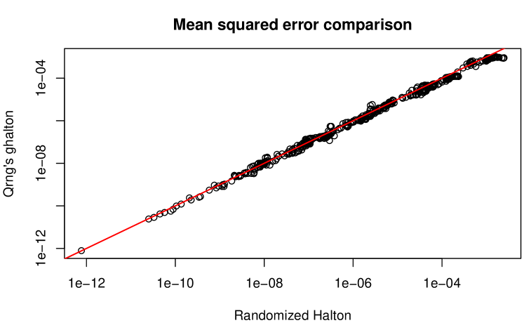
Figure 12: The horizontal axis has mean squared errors from rhalton. The vertical axis has mean squared errors for the ghalton program from the R package qrng. There is a reference line where the MSEs are equal.

The ghalton code does not come with internal seeding methods. Version 0.0-3 allows up to $d=360$ dimensions. If the seed is set and $n$ and $d$ are increased, the new matrix contains the previous one as its upper left corner:

> set.seed(1);x1=ghalton(500,180);set.seed(1);x2=ghalton(1000,360)
> range(x2[1:500,1:180]-x1)
[1] 0 0

The principal advantage of the present rhalton code is that it can be extended to $n^{\prime}>n$ rows only computing the new $n^{\prime}-n$ rows, or to $d^{\prime}>d$ columns only computing the new $d^{\prime}-d$ columns. It is even possible to extract an arbitrary single element ${\mathcal{X}}^{(s)}_{ij}$ via rhalton(1,1,n0=i-1,d0=j-1,singleseed=s). A second advantage is that the pseudocode is so simple that one can easily write it in a new language, such as julia (Bezanson et al.,, 2017), or use it for instructional purposes about RQMC.

There are more accurate RQMC methods than this one, if the integrand has sufficient smoothness. See, for instance Dick, (2011) or Owen, (1997). However any rule with error or root mean squared error $o(1/n)$ cannot be reasonably used at arbitrary sample sizes. To see why, suppose that $\hat{\mu}_{n}$ is an average of $n$ evaluations and $\hat{\mu}_{n+1}$ averages $n+1$ of them. Then $\hat{\mu}_{n+1}-\hat{\mu}_{n}=O(1/n)$. If $\hat{\mu}_{n}$ had error $o(1/n)$ then we have probably made it an order of magnitude worse just by taking one more observation. The only exception would be if $f(x_{n+1})$ itself had error $o(1/n)$. In that case we would just use $f(x_{n+1})$ all by itself. This observation is due to Sobol’, (1998) and was worked out in detail in Owen, (2015). The consequence is that for $o(1/n)$ accuracy an equal weight rule must use sample sizes $n_{\ell}$ with some lower bound on $n_{\ell+1}/n_{\ell}$. Equal weight rules with arbitrary sample sizes are easiest to use.

Nested uniform scrambling of $(t,m,d)$-nets in base $b$ (Owen,, 1995) has the property that for finite $n$ the resulting variance cannot be much worse than plain MC for any integrand $f$ in $L^{2}$. The bound depends on $t,m,d$ and $b$ for sample sizes $n=b^{m}$. The randomized Halton method presented here does not have that property. Pathological exceptions are possible. Suppose that $d=26$ and that $f(x_{i})$ only depends on the $26$’th component $x_{ij}$. The $26$’th prime is $101$ and to make matters worse, suppose that $f(x_{i})$ is a periodic function of $x_{i,26}$ with period $1/101$. Then the first $101$ values of $f(x_{i})$ are all equal. So are the second $101$ values. The variance could be $101$ times as large as Monte Carlo sampling, and of course a larger prime number would be even more problematic, as would a function that depended only on $x_{j}$ and had period $p_{j}^{k}$ for some $k$. The code presented here is based on ignoring this far-fetched possibility for the sake of simplicity of implementation and use.

Appendix: source code in R

#
# Coded by Art B. Owen, Stanford University.
# April 2017
#
rhalton <- function(n,d,n0=0,d0=0,singleseed,seedvector){
#
# Randomly scrambled Halton sequence of n points in d dimensions.
#
# If you already have n0 old points, set n0 to get the next n points.
# If you already have d0 old components, set d0 to get the next d inputs.
# Get points  n0 + 0:(n-1)  in dimensions  d0 + (1:d)
#
# seedvector  = optional vector of  d0+d random seeds, one per dimension
# singleseed  = optional scalar seed (has lower precedence than seedvector)

# Handle input dimension correctness and corner cases
  if( min(n0,d0) < 0 )
    stop(paste("Starting indices (n0, d0) cannot be < 0, input had (",n0,",",d0,")"))
  if( min(n,d) < 0 )
    stop(paste("Cannot have negative n or d"))
  if( n==0 || d==0 ) # Odd corner cases: user wants n x 0 or 0 x d matrix.
    return(matrix(nrow=n,ncol=d))
  D <- nthprime(0,getlength=TRUE)
  if( d0+d > D )
    stop(paste("Implemented only for d <=",D))

# Seed rules
  if( !missing(singleseed) && length(singleseed) != 1 )
    stop("singleseed, if supplied, must be scalar")
  if( !missing(seedvector) && length(seedvector) < d0+d )
    stop("seedvector, if supplied, must be have length at least d0+d")
  if(  missing(seedvector) && !missing(singleseed) )
    seedvector <- singleseed + 1:(d0+d) - 1

# Generate and return the points
  ans <- matrix(0,n,d)
  for( j in 1:d ){
    dimj <- d0+j
    if( !missing(seedvector) )set.seed(seedvector[dimj])
    ans[,j] <- randradinv( n0 + 0:(n-1), nthprime(dimj) )  # zero indexed rows
  }
  ans
}

randradinv <- function(ind,b=2){
# Randomized radical inverse functions for indices in ind and for base b.
# The calling routine should set the random seed if reproducibility is desired.

  if(any(ind!=round(ind)))
    stop("Indices have to be integral.")
  if(any(ind<0))
    stop("Indices cannot be negative.")
  if(!(is.vector(b) && length(b)==1 && b==floor(b) && b>1))
    stop("b must be a single integer >= 2")

  b2r <- 1/b
  ans <- ind*0
  res <- ind
  while( 1-b2r < 1 ){  # Assumes floating point comparisons, fixed precision.
    dig  <- res %% b
    perm <- sample(b)-1
    pdig <- perm[1+dig]
    ans  <- ans + pdig * b2r
    b2r  <- b2r/b
    res  <- (res - dig)/b
  }
  ans
}

nthprime <- function(n,getlength=FALSE){
# Get the n’th prime, using a hard coded list (or get the length of that list).

# First fifty-eight prime numbers from OEIS A000040, April 2017
primes <- c( 2,   3,   5,   7,  11,  13,  17,  19,  23,  29,
            31,  37,  41,  43,  47,  53,  59,  61,  67,  71,
            73,  79,  83,  89,  97, 101, 103, 107, 109, 113,
           127, 131, 137, 139, 149, 151, 157, 163, 167, 173,
           179, 181, 191, 193, 197, 199, 211, 223, 227, 229,
           233, 239, 241, 251, 257, 263, 269, 271)

# First 1000 prime numbers from primes.utm.edu/lists/small/1000.txt, April 2017
primes <- c(
     2,    3,    5,    7,   11,   13,   17,   19,   23,   29
,   31,   37,   41,   43,   47,   53,   59,   61,   67,   71
,   73,   79,   83,   89,   97,  101,  103,  107,  109,  113
,  127,  131,  137,  139,  149,  151,  157,  163,  167,  173
,  179,  181,  191,  193,  197,  199,  211,  223,  227,  229
,  233,  239,  241,  251,  257,  263,  269,  271,  277,  281
,  283,  293,  307,  311,  313,  317,  331,  337,  347,  349
,  353,  359,  367,  373,  379,  383,  389,  397,  401,  409
,  419,  421,  431,  433,  439,  443,  449,  457,  461,  463
,  467,  479,  487,  491,  499,  503,  509,  521,  523,  541
,  547,  557,  563,  569,  571,  577,  587,  593,  599,  601
,  607,  613,  617,  619,  631,  641,  643,  647,  653,  659
,  661,  673,  677,  683,  691,  701,  709,  719,  727,  733
,  739,  743,  751,  757,  761,  769,  773,  787,  797,  809
,  811,  821,  823,  827,  829,  839,  853,  857,  859,  863
,  877,  881,  883,  887,  907,  911,  919,  929,  937,  941
,  947,  953,  967,  971,  977,  983,  991,  997, 1009, 1013
, 1019, 1021, 1031, 1033, 1039, 1049, 1051, 1061, 1063, 1069
, 1087, 1091, 1093, 1097, 1103, 1109, 1117, 1123, 1129, 1151
, 1153, 1163, 1171, 1181, 1187, 1193, 1201, 1213, 1217, 1223
, 1229, 1231, 1237, 1249, 1259, 1277, 1279, 1283, 1289, 1291
, 1297, 1301, 1303, 1307, 1319, 1321, 1327, 1361, 1367, 1373
, 1381, 1399, 1409, 1423, 1427, 1429, 1433, 1439, 1447, 1451
, 1453, 1459, 1471, 1481, 1483, 1487, 1489, 1493, 1499, 1511
, 1523, 1531, 1543, 1549, 1553, 1559, 1567, 1571, 1579, 1583
, 1597, 1601, 1607, 1609, 1613, 1619, 1621, 1627, 1637, 1657
, 1663, 1667, 1669, 1693, 1697, 1699, 1709, 1721, 1723, 1733
, 1741, 1747, 1753, 1759, 1777, 1783, 1787, 1789, 1801, 1811
, 1823, 1831, 1847, 1861, 1867, 1871, 1873, 1877, 1879, 1889
, 1901, 1907, 1913, 1931, 1933, 1949, 1951, 1973, 1979, 1987
, 1993, 1997, 1999, 2003, 2011, 2017, 2027, 2029, 2039, 2053
, 2063, 2069, 2081, 2083, 2087, 2089, 2099, 2111, 2113, 2129
, 2131, 2137, 2141, 2143, 2153, 2161, 2179, 2203, 2207, 2213
, 2221, 2237, 2239, 2243, 2251, 2267, 2269, 2273, 2281, 2287
, 2293, 2297, 2309, 2311, 2333, 2339, 2341, 2347, 2351, 2357
, 2371, 2377, 2381, 2383, 2389, 2393, 2399, 2411, 2417, 2423
, 2437, 2441, 2447, 2459, 2467, 2473, 2477, 2503, 2521, 2531
, 2539, 2543, 2549, 2551, 2557, 2579, 2591, 2593, 2609, 2617
, 2621, 2633, 2647, 2657, 2659, 2663, 2671, 2677, 2683, 2687
, 2689, 2693, 2699, 2707, 2711, 2713, 2719, 2729, 2731, 2741
, 2749, 2753, 2767, 2777, 2789, 2791, 2797, 2801, 2803, 2819
, 2833, 2837, 2843, 2851, 2857, 2861, 2879, 2887, 2897, 2903
, 2909, 2917, 2927, 2939, 2953, 2957, 2963, 2969, 2971, 2999
, 3001, 3011, 3019, 3023, 3037, 3041, 3049, 3061, 3067, 3079
, 3083, 3089, 3109, 3119, 3121, 3137, 3163, 3167, 3169, 3181
, 3187, 3191, 3203, 3209, 3217, 3221, 3229, 3251, 3253, 3257
, 3259, 3271, 3299, 3301, 3307, 3313, 3319, 3323, 3329, 3331
, 3343, 3347, 3359, 3361, 3371, 3373, 3389, 3391, 3407, 3413
, 3433, 3449, 3457, 3461, 3463, 3467, 3469, 3491, 3499, 3511
, 3517, 3527, 3529, 3533, 3539, 3541, 3547, 3557, 3559, 3571
, 3581, 3583, 3593, 3607, 3613, 3617, 3623, 3631, 3637, 3643
, 3659, 3671, 3673, 3677, 3691, 3697, 3701, 3709, 3719, 3727
, 3733, 3739, 3761, 3767, 3769, 3779, 3793, 3797, 3803, 3821
, 3823, 3833, 3847, 3851, 3853, 3863, 3877, 3881, 3889, 3907
, 3911, 3917, 3919, 3923, 3929, 3931, 3943, 3947, 3967, 3989
, 4001, 4003, 4007, 4013, 4019, 4021, 4027, 4049, 4051, 4057
, 4073, 4079, 4091, 4093, 4099, 4111, 4127, 4129, 4133, 4139
, 4153, 4157, 4159, 4177, 4201, 4211, 4217, 4219, 4229, 4231
, 4241, 4243, 4253, 4259, 4261, 4271, 4273, 4283, 4289, 4297
, 4327, 4337, 4339, 4349, 4357, 4363, 4373, 4391, 4397, 4409
, 4421, 4423, 4441, 4447, 4451, 4457, 4463, 4481, 4483, 4493
, 4507, 4513, 4517, 4519, 4523, 4547, 4549, 4561, 4567, 4583
, 4591, 4597, 4603, 4621, 4637, 4639, 4643, 4649, 4651, 4657
, 4663, 4673, 4679, 4691, 4703, 4721, 4723, 4729, 4733, 4751
, 4759, 4783, 4787, 4789, 4793, 4799, 4801, 4813, 4817, 4831
, 4861, 4871, 4877, 4889, 4903, 4909, 4919, 4931, 4933, 4937
, 4943, 4951, 4957, 4967, 4969, 4973, 4987, 4993, 4999, 5003
, 5009, 5011, 5021, 5023, 5039, 5051, 5059, 5077, 5081, 5087
, 5099, 5101, 5107, 5113, 5119, 5147, 5153, 5167, 5171, 5179
, 5189, 5197, 5209, 5227, 5231, 5233, 5237, 5261, 5273, 5279
, 5281, 5297, 5303, 5309, 5323, 5333, 5347, 5351, 5381, 5387
, 5393, 5399, 5407, 5413, 5417, 5419, 5431, 5437, 5441, 5443
, 5449, 5471, 5477, 5479, 5483, 5501, 5503, 5507, 5519, 5521
, 5527, 5531, 5557, 5563, 5569, 5573, 5581, 5591, 5623, 5639
, 5641, 5647, 5651, 5653, 5657, 5659, 5669, 5683, 5689, 5693
, 5701, 5711, 5717, 5737, 5741, 5743, 5749, 5779, 5783, 5791
, 5801, 5807, 5813, 5821, 5827, 5839, 5843, 5849, 5851, 5857
, 5861, 5867, 5869, 5879, 5881, 5897, 5903, 5923, 5927, 5939
, 5953, 5981, 5987, 6007, 6011, 6029, 6037, 6043, 6047, 6053
, 6067, 6073, 6079, 6089, 6091, 6101, 6113, 6121, 6131, 6133
, 6143, 6151, 6163, 6173, 6197, 6199, 6203, 6211, 6217, 6221
, 6229, 6247, 6257, 6263, 6269, 6271, 6277, 6287, 6299, 6301
, 6311, 6317, 6323, 6329, 6337, 6343, 6353, 6359, 6361, 6367
, 6373, 6379, 6389, 6397, 6421, 6427, 6449, 6451, 6469, 6473
, 6481, 6491, 6521, 6529, 6547, 6551, 6553, 6563, 6569, 6571
, 6577, 6581, 6599, 6607, 6619, 6637, 6653, 6659, 6661, 6673
, 6679, 6689, 6691, 6701, 6703, 6709, 6719, 6733, 6737, 6761
, 6763, 6779, 6781, 6791, 6793, 6803, 6823, 6827, 6829, 6833
, 6841, 6857, 6863, 6869, 6871, 6883, 6899, 6907, 6911, 6917
, 6947, 6949, 6959, 6961, 6967, 6971, 6977, 6983, 6991, 6997
, 7001, 7013, 7019, 7027, 7039, 7043, 7057, 7069, 7079, 7103
, 7109, 7121, 7127, 7129, 7151, 7159, 7177, 7187, 7193, 7207
, 7211, 7213, 7219, 7229, 7237, 7243, 7247, 7253, 7283, 7297
, 7307, 7309, 7321, 7331, 7333, 7349, 7351, 7369, 7393, 7411
, 7417, 7433, 7451, 7457, 7459, 7477, 7481, 7487, 7489, 7499
, 7507, 7517, 7523, 7529, 7537, 7541, 7547, 7549, 7559, 7561
, 7573, 7577, 7583, 7589, 7591, 7603, 7607, 7621, 7639, 7643
, 7649, 7669, 7673, 7681, 7687, 7691, 7699, 7703, 7717, 7723
, 7727, 7741, 7753, 7757, 7759, 7789, 7793, 7817, 7823, 7829
, 7841, 7853, 7867, 7873, 7877, 7879, 7883, 7901, 7907, 7919
)

p <- length(primes)
if( getlength )
  return(p)
if( any(n<1) )
  stop(paste(sep="","The n’th prime is only available for n >= 1, not n = ",min(n)))
if( any(n>p) )
  stop(paste(sep="","The present list of primes has length ",p,
   ". It does not include the n’th one for n = ",max(n),"."))

return(primes[n])
}

References

- Aistleitner and Dick, (2014) Aistleitner, C. and Dick, J. (2014). Functions of bounded variation, signed measures, and a general Koksma-Hlawka inequality. Technical Report arXiv1406.0230, University of New South Wales.
- Atanassov, (2004) Atanassov, E. (2004). On the discrepancy of the Halton sequence. Mathematica Balkanica, 18:15–32.
- Bezanson et al., (2017) Bezanson, J., Edelman, A., Karpinski, S., and Shah, V. B. (2017). Julia: A fresh approach to numerical computing. SIAM Review, 59(1):65–98.
- Borchers, (2017) Borchers, H. W. (2017). numbers: Number-Theoretic Functions. R package version 0.6-6.