Learning to Embed Words in Context for Syntactic Tasks

Abstract

We present models for embedding words in the context of surrounding words. Such models, which we refer to as token embeddings, represent the characteristics of a word that are specific to a given context, such as word sense, syntactic category, and semantic role. We explore simple, efficient token embedding models based on standard neural network architectures. We learn token embeddings on a large amount of unannotated text and evaluate them as features for part-of-speech taggers and dependency parsers trained on much smaller amounts of annotated data. We find that predictors endowed with token embeddings consistently outperform baseline predictors across a range of context window and training set sizes.

1 Introduction

Word embeddings have enjoyed a surge of popularity in natural language processing (NLP) due to the effectiveness of deep learning and the availability of pretrained, downloadable models for embedding words. Many embedding models have been developed Collobert et al. (2011); Mikolov et al. (2013); Pennington et al. (2014) and have been shown to improve performance on NLP tasks, including part-of-speech (POS) tagging, named entity recognition, semantic role labeling, dependency parsing, and machine translation Turian et al. (2010); Collobert et al. (2011); Bansal et al. (2014); Zou et al. (2013).

The majority of this work has focused on a single embedding for each word type in a vocabulary. We will refer to these as type embeddings. However, the same word type can exhibit a range of linguistic behaviors in different contexts. To address this, some researchers learn multiple embeddings for certain word types, where each embedding corresponds to a distinct sense of the type Reisinger and Mooney (2010); Huang et al. (2012); Tian et al. (2014). But token-level linguistic phenomena go beyond word sense, and these approaches are only reliable for frequent words.

Several kinds of token-level phenomena relate directly to NLP tasks. Word sense disambiguation relies on context to determine which sense is intended. POS tagging, dependency parsing, and semantic role labeling identify syntactic categories and semantic roles for each token. Sentiment analysis and related tasks like opinion mining seek to understand word connotations in context.

In this paper, we develop and evaluate models for embedding word tokens. Our token embeddings capture linguistic characteristics expressed in the context of a token. Unlike type embeddings, it is infeasible to precompute and store all possible (or even a significant fraction of) token embeddings. Instead, our token embedding models are parametric, so they can be applied on the fly to embed any word in its context.

We focus on simple and efficient token embedding models based on local context and standard neural network architectures. We evaluate our models by using them to provide features for downstream low-resource syntactic tasks: Twitter POS tagging and dependency parsing. We show that token embeddings can improve the performance of a non-structured POS tagger to match the state of the art Twitter POS tagger of Owoputi et al. (2013). We add our token embeddings to Tweeboparser Kong et al. (2014), improving its performance and establishing a new state of the art for Twitter dependency parsing.

2 Related Work

The most common way to obtain context-sensitive embeddings is to learn separate embeddings for distinct senses of each type. Most of these methods cluster tokens into senses and learn vectors for each cluster Vu and Parker (2016); Reisinger and Mooney (2010); Huang et al. (2012); Tian et al. (2014); Chen et al. (2014); Piña and Johansson (2015); Wu and Giles (2015). Some use bilingual information Guo et al. (2014); Šuster et al. (2016); Gonen and Goldberg (2016), nonparametric methods to avoid specifying the number of clusters Neelakantan et al. (2014); Li and Jurafsky (2015), topic models Liu et al. (2015), grounding to WordNet Jauhar et al. (2015), or senses defined as sets of POS tags for each type Qiu et al. (2014).

These “multi-type” embeddings are restricted to modeling phenomena expressed by a single clustering of tokens for each type. In contrast, token embeddings are capable of modeling information that cuts across phenomena categories. Further, as the number of clusters grows, learning multi-type embeddings becomes more difficult due to data fragmentation. Instead, we learn parametric models that transform a type embedding and those of its context words into a representation for the token. While multi-type embeddings require more data for training, parametric models require less.

There is prior work in developing representations for tokens in the context of unsupervised or supervised training, whether with long short-term memory (LSTM) networks Kågebäck et al. (2015); Ling et al. (2015); Choi et al. (2016); Melamud et al. (2016), convolutional networks Collobert et al. (2011), or other architectures. However, learning to represent tokens in supervised training can suffer from limited data. We instead focus on learning token embedding models on unlabeled data, then use them to produce features for downstream tasks. So we focus on efficient architectures and unsupervised learning criteria.

The most closely related work consists of efforts to train LSTMs to represent tokens in context using unsupervised training objectives. Kawakami and Dyer (2015) use multilingual data to learn token embeddings that are predictive of their translation targets, while Melamud et al. (2016) and Peters et al. (2017) use unsupervised learning with monolingual sentences. We experiment with LSTM token embedding models as well, though we focus on different tasks: POS tagging and dependency parsing. We generally found that very small contexts worked best for these syntactic tasks, thereby limiting the usefulness of LSTMs as token embedding models.

3 Token Embedding Models

We assume access to pretrained type embeddings. Let $\mathcal{W}$ denote a vocabulary of word types. For each word type $x\in\mathcal{W}$, we denote its type embedding by $\mbox{\boldmath$v$}_{x}\in\mathbb{R}^{d}$.

We define a word sequence $\mbox{\boldmath$x$}=\langle x_{1},x_{2},...,x_{|\mbox{\boldmath$x$}|}\rangle$ in which each entry $x_{j}$ is a word type, i.e., $x_{j}\in\mathcal{W}$. We define a word token as an element in a word sequence. We consider the class of functions $f$ that take a word sequence $x$ and index $j$ of a particular token in $x$ and output a vector of dimensionality $d^{\prime}$. We will refer to choices for $f(\mbox{\boldmath$x$},j)$ as encoders.

3.1 Feedforward Encoders

Our first encoder is a basic feedforward neural network that embeds the sequence of words contained in a window of text surrounding word $j$. We use a fixed-size window containing word $j$, the $w^{\prime}$ words to its left, and the $w^{\prime}$ words to its right. We concatenate the vectors for each word type in this window and apply an affine transformation followed by a nonlinearity:

$$f_{\mathrm{FF}}(\mbox{\boldmath$x$},j)=$$

$$g\left(W^{(D)}[\mbox{\boldmath$v$}_{x_{j-w^{\prime}}};\mbox{\boldmath$v$}_{x_{(j-w^{\prime})+1}};...;\mbox{\boldmath$v$}_{x_{j+w^{\prime}}}]+\mbox{\boldmath$b$}^{(D)}\right)$$

where $g$ is an elementwise nonlinear function (e.g., $\tanh$), $W^{(D)}$ is a $d^{\prime}$ by $d(2w^{\prime}+1)$ parameter matrix, semicolon (;) denotes vertical concatenation, and $\mbox{\boldmath$b$}^{(D)}\in\mathbb{R}^{d^{\prime}}$ is a bias vector. We assume that $x$ is padded with start-of-sequence and end-of-sequence symbols as needed. The resulting $d^{\prime}$-dimensional token embedding can be transformed by additional nonlinear layers.

This encoder does not distinguish word $j$ other than by centering the window at its position. It is left to the training objectives to place emphasis on word $j$ as needed (see Section 3.3). Varying $w^{\prime}$ will influence the phenomena captured by this encoder, with smaller windows capturing similarity in terms of local syntactic category (e.g., noun vs. verb) and larger windows helping to distinguish word senses or to identify properties of the discourse (e.g., topic or style).

3.2 Recurrent Neural Network Encoders

The above feedforward DNN encoder will be brittle with large window sizes. We therefore also consider encoders based on recurrent neural networks (RNNs). RNNs have recently enjoyed a great deal of interest in the deep learning, speech recognition, and NLP communities Sundermeyer et al. (2012); Graves et al. (2013); Sutskever et al. (2014), most frequently used with “gated” connections like long short-term memory (LSTM) Hochreiter and Schmidhuber (1997); Gers et al. (2000).

We use an LSTM to encode the sequence of words containing the token and take the final hidden vector as the $d^{\prime}$-dimensional encoding. While we can use longer sequences, such as the sentence containing the token Kawakami and Dyer (2015), we restrict the input sequence to a fixed-size context window around word $j$, so the input is identical to that of the feedforward encoder above. For the syntactic tasks we consider, we did not find large context windows to be helpful.

3.3 Training

We consider unsupervised ways to train the encoders described above. Throughout training for both models, the type embeddings are kept fixed. We assume that we are given a corpus $X=\{\mbox{\boldmath$x$}^{(i)}\}_{i=1}^{|X|}$ of unannotated word sequences.

One widely-used family of unsupervised criteria is that of reconstruction error and its variants. These are used when training autoencoders, which use an encoder $f$ to convert the input $x$ to a vector followed by a decoder $g$ that attempts to reconstruct the input from the vector. The typical loss function is the squared difference between the input and reconstructed input. We use a generalization that is sensitive to the position of elements. Since our primary interest is in learning useful representations for a particular token in its context, we use a weighted reconstruction error:

$$\mathrm{loss}_{\mathrm{WRE}}(f,g,\mbox{\boldmath$x$},j)=\sum_{i=1}^{|\mbox{\boldmath$x$}|}\omega_{i}\left\|g(f(\mbox{\boldmath$x$},j))_{i}-\mbox{\boldmath$v$}_{x_{i}}\right\|_{2}^{2}$$ (1)

where $g(f(\mbox{\boldmath$x$},j))_{i}$ is the subvector of $g(f(\mbox{\boldmath$x$},j))$ corresponding to reconstructing $\mbox{\boldmath$v$}_{x_{i}}$, and where $\omega_{i}$ is the weight for reconstructing the $i$th entry.

For our feedforward encoder $f$, we use analogous fully-connected layers in the decoder $g$, forming a standard autoencoder architecture. To train the LSTM encoder, we add an LSTM decoder to form a sequence-to-sequence (“seq2seq”) autoencoder Sutskever et al. (2014); Li et al. (2015); Dai and Le (2015). That is, we use one LSTM as the encoder $f$ and another LSTM for the decoder $g$, initializing $g$’s hidden state to the output of $f$. Since we use the same weighted reconstruction error described above, the decoder must output a single vector at each step rather than a distribution over word types. So we use an affine transformation on the LSTM decoder hidden vector at each step in order to generate the output vector for each step. Reconstruction error has efficiency advantages over log loss here in that it avoids the costly summation over the vocabulary.

4 Qualitative Analysis

Before discussing downstream tasks, we perform a qualitative analysis to show what our token embedding models learn.

Q	my first one was like 2 minutes long and has	Q	jus listenin 2 mr hudson and drake crazyness
1	my fav place- was there 2 years ago and am	1	@mention deaddddd u go 2 mlk high up n
2	thought it was more like 2 ….. either way , i	2	only a cups tho tryin 2 feed the whole family
3	to backup everything from 2 years before i	3	bored on mars i kum down 2 earth … yupp !!
4	i slept for like 2 sec lol . freakin chessy	4	i miss you i trying 2 looking oud my mind girl
Q	the lines : i am so thrilled about this . may	Q	fighting off a headache so i can work on my
1	and work . i am so glad you asked . let	1	im on my phone so i cant see who @mention
2	i was so excited to sleep in tomorrow	2	did some things that hurt so i guess i was doing
3	@mention that is so funny ! i know which	3	my phone keeps beeping so i know ralph must
4	little girl ! i was so touched when she called	4	randomly obsessed with this song so i bought it

Table 1: Query tokens of two polysemous words and their four nearest neighboring tokens. The target token is underlined and the encoder context (3 words to either side) is shown in bold. See text for details.

4.1 Experimental Setup

We train a feedforward DNN token embedding model on a corpus of 300,000 unlabeled English tweets. We use a window size $w^{\prime}=3$ for the qualitative results reported here; for downstream tasks below, we will vary $w^{\prime}$. For training, we use our weighted reconstruction error (Eq. 1). The encoder uses one hidden layer of size 512 followed by the token embedding layer of size $d^{\prime}=256$. The decoder also uses a single hidden layer of size 512. We use ReLU activations except the final encoder/decoder layers which use linear activations.

In preliminary experiments we compared 3 weighting schemes for $\omega$ in the objective: for token index $j$, “uniform” weighting sets $\omega_{i}=1$ for all $i$; “focused” sets $\omega_{j}=2$ and $\omega_{i}=1$ for $i\neq j$; and “tapered” sets $\omega_{j}=4$, $\omega_{j\pm 1}=3$, $\omega_{j\pm 2}=2$, and 1 otherwise. The non-uniform schemes place more emphasis on reconstructing the target token, and we found them to slightly outperform uniform weighting. Unless reported otherwise, we use focused weighting for all experiments below.

We train using stochastic gradient descent with momentum for 1 epoch, saving the model that reaches the best objective value on a held-out validation set of 3,000 unlabeled tweets. For the type embeddings used as input to our token embedding model, we train 100-dimensional skip-gram embeddings on 56 million English tweets using the word2vec toolkit Mikolov et al. (2013).

4.2 Nearest Neighbor Analysis

We inspect the ability of the encoder to distinguish different senses of ambiguous types. Table 1 shows query tokens (Q) followed by their four nearest neighbor tokens (with the same type), all from our held-out set of 3,000 tweets. We choose two polysemous words that are common in tweets: “2” and “so”. As queries, we select tokens that express different senses. The word “2” can be both a number (left) and a synonym of “to” (right). The word “so” is both an intensifier (left) and a connective (right). We find that the nearest neighbors, though generally differing in context words, have the same sense and same POS tag.

In Table 2 we consider nearest neighbors that may have different word types from the query type. For each query word, we permit the nearest neighbor search to consider tokens from the following set: {“4”, “for”, “2”, “to”, “too”, “1”, “one”}. In the first two queries, we find that tokens of “4” have nearest neighbors with different word types but the same syntactic category. That is, tokens of different word types are more similar to the query than tokens of the same type. We see this again with neighbors of “2” used as a synonym for “to”. The encoder appears to be doing a kind of canonicalization of nonstandard word uses, which suggests applications for token embeddings in normalization of social media text Clark and Araki (2011). See neighbor 8, in which “too” is understood as having the intended meaning despite its misleading surface form.

Q	masters swimmers annual swim 4 your heart !
1	so many miles loking for her and handing
2	off to the rehearsal space for a weekend long
3	on the inauguration for your enjoyment
Q	#canucks now have a 4 point lead on the
1	way lol . it’s the 1 mile trail and then you
2	my first one was like 2 minutes long and
3	my fav place- was there 2 years ago and
Q	jus listenin 2 mr hudson and drake crazyness
1	@mention deaddddd u go 2 mlk high up n bk
2	only a cups tho tryin 2 feed the whole family
3	are ya’ll listening to the annointed one ? he’s on
4	@mention well could u come to mrs wilsons for
5	i’m bored on mars i kum down 2 earth … yupp !!
6	i am listening to amar prtihibi - black
7	about neopets and listening to yelle ( URL
8	high ritee now -______- bout too troop to the crib

Table 2: Nearest neighbors for token embeddings, where we consider neighbors that may have different word types from that in the query token. See text for details.

4.3 Visualization

In order to gain a better qualitative understanding of the token embeddings, we visualize the learned token embeddings using t-SNE Maaten and Hinton (2008). We learn token embeddings as above except with $w^{\prime}=1$. Figure 1 shows a two-dimensional visualization of token embeddings for the word type “4”. For this visualization, we embed tokens in the POS-annotated tweet datasets from Gimpel et al. (2011) and Owoputi et al. (2013), so we have their gold standard POS tags. We show the left and right context words (using $w^{\prime}=1$) along with the token and its gold standard POS tag. We find that tokens of “4” with the same gold POS tag are close in the embedded space, with prepositions appearing in the upper part of the plot and numbers appearing in the lower part.

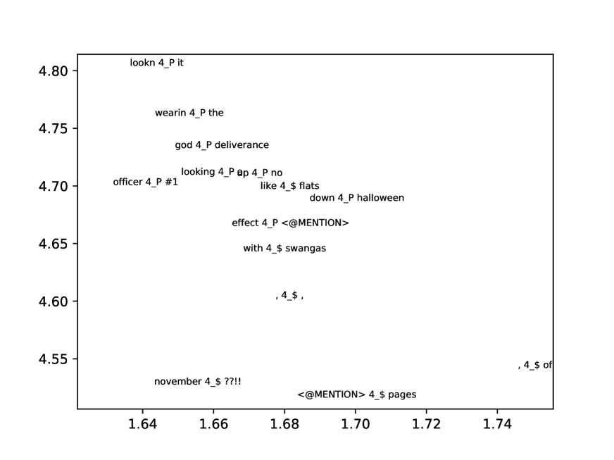
Figure 1: t-SNE visualization of token embeddings for word type “4”. Each point shows the left and right context words ($w^{\prime}=1$) for the token along with the gold standard POS tag following an underscore (“_”). The tag “P” is preposition and “$” is number. Following the t-SNE projection, points were subsampled for this visualization for clarity.

5 Downstream Tasks

We evaluate our token embedding models on two downstream tasks: POS tagging and dependency parsing. Given an input sequence $\mbox{\boldmath$x$}=\langle x_{1},x_{2},...,x_{n}\rangle$, we want to predict its tag sequence and dependency parse. We focus on Twitter since there is limited annotated data but abundant unlabeled data for training token embeddings.

5.1 Part-of-Speech Tagging

Baseline

We use a simple feedforward DNN as our baseline tagger. It is a local classifier that predicts the tag for a token independently of all other predictions for the tweet. That is, it does not use structured prediction. The input to the network is the type embedding of the word to be tagged concatenated with the type embeddings of $w$ words on either side. The DNN contains two hidden layers followed by one softmax layer. Figure 2(a) shows this architecture for $w=1$ when predicting the tag of 4 in the tweet thanks 4 follow. We concatenate a 10-dimensional binary feature vector computed for the word being tagged (Table 3).

(a) Baseline DNN Tagger

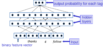
(b) Token Embedding Tagger

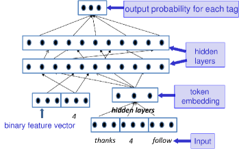
Figure 2: (a) Baseline DNN tagger, (b) tagger augmented with token embeddings.

$x$ begins with @ and $|x|>1$

$x$ begins with # and $|x|>1$

$\mathrm{lowercase}(x)$ is rt (retweet indicator)

$x$ matches URL regular expression

$x$ only contains digits

$x$ contains $

$x$ is : (colon)

$x$ is …(ellipsis)

$x$ is punctuation and $|x|=1$ and x is not : or $

$x$ is punctuation and $|x|>1$ and x is not …

Table 3: Rules for binary feature vector for word $x$. If multiple rules apply, the first has priority. The tagger uses this feature vector only for the word to be tagged; the parser uses one for the child and another for the parent in the dependency arc under consideration.

We train the tagger by minimizing the log loss (cross entropy) on the training set, performing early stopping on the validation set, and reporting accuracy on the test set. We consider both learning the type embeddings (“updating”) and keeping them fixed. When we update the embeddings we include an $\ell_{2}$ regularization term penalizing the divergence from the initial type embeddings.

Token Embedding Tagger

When using token embeddings, we concatenate the $d^{\prime}$-dimensional token embedding to the tagger input. The rest of the architecture is the same as the baseline tagger. Figure 2(b) shows the model when using type embedding window size $w=0$ and token embedding window size $w^{\prime}=1$.

While training the DNN tagger with the token embeddings, we do not fine-tune the token embedding encoder parameters, leaving them fixed.

5.2 Dependency Parser

$\frac{i}{n}$

$\frac{j}{n}$

$\Delta=1$

$\Delta=2$

$3\leq\Delta\leq 5$

$6\leq\Delta\leq 10$

$\Delta\geq 11$

$i<j$

$i>j$

$x_{j}$ is wall symbol

Table 4: Dependency pair features for arc with child $x_{i}$ and parent $x_{j}$ in an $n$-word sentence and where $\Delta=|i-j|$. The final feature is 1 if $x_{j}$ is the wall symbol ($), indicating a root attachment for $x_{i}$. In that case, all features are zero except for the first and last.

Baseline

As our baseline, we use a simple DNN to do parent prediction independently for each word. That is, we use a local classifier that scores parents for a word. To infer a parse at test time, we independently choose the highest-scoring parent for each word. We also use our classifier’s scores as additional features in TweeboParser Kong et al. (2014).

Our parent prediction DNN has two hidden layers and an output layer with 1 unit. This unit corresponds to a value $S(x_{i},x_{j})$ that serves as the score for a dependency arc with child word $x_{i}$ and parent word $x_{j}$. The input to the DNN is the concatenation of the type embeddings for $x_{i}$ and $x_{j}$, the type embeddings of $w$ words on either side of $x_{i}$ and $x_{j}$, the features for $x_{i}$ and $x_{j}$ from Table 3, and features for the pair, including relative positions, direction, and distance (shown in Table 4).

For a sentence of length $n$, the loss function we use for a single arc $(x_{i},x_{j})$ follows:

$$\mathrm{loss}_{\mathrm{arc}}(x_{i},x_{j})=$$

$$\;-S(x_{i},x_{j})+\log\left(\sum_{k=0,k\neq i}^{n}\!\!\!\exp\{S(x_{i},x_{k})\}\right)$$ (2)

where $k=0$ indicates the root attachment for $x_{i}$. We sum over all possible parents even though the model only computes a score for a binary decision. Where $\mathrm{head}(x_{i})$ returns the annotated parent for $x_{i}$, the loss for a sequence $x$ is:

$$\sum_{i=1}^{n}\mathrm{loss}_{\mathrm{arc}}(x_{i},\mathrm{head}(x_{i}))$$ (3)

After training, we predict the parent for a word $x_{i}$

as follows:

$$\overline{\mathrm{head}}(x_{i})=\operatornamewithlimits{argmax}_{k\neq i}S(x_{i},x_{k})$$ (4)

Token Embedding Parser

For the token embedding parser, we use the $d^{\prime}$-dimensional token embeddings for $x_{i}$ and $x_{j}$. We simply concatenate the two token embeddings to the input of the DNN parser. When $x_{j}=\$$, the token embedding for $x_{j}$ is all zeroes. The other parts of the input are the same as the baseline parser. While training this parser, we do not optimize the token embedding encoder parameters. As with the tagger, we tune over the decision to keep type embeddings fixed or update them during learning, again using $\ell_{2}$ regularization when doing so. We tune this decision for both the baseline parser and the parser that uses token embeddings.

6 Experimental Setup

For training the token embedding models, we mostly use the same settings as in Section 4.1 for the qualitative analysis. The only difference is that we train the token embedding models for 5 epochs, again saving the model that reaches the best objective value on a held-out set of 3,000 unlabeled tweets. We also experiment with several values for the context window size $w^{\prime}$ and the hidden layer size, reported below.

6.1 Part-of-Speech Tagging

We use the annotated tweet datasets from Gimpel et al. (2011) and Owoputi et al. (2013). For training, we combine the 1000-tweet Oct27Train set and the 327-tweet Oct27Dev development set. For validation, we use the 500-tweet Oct27Test test set and for final testing we use the 547-tweet Daily547 test set. The DNN tagger uses two hidden layers of size 512 with ReLU nonlinearities and a final softmax layer of size 25 (one for each tag). The input type embeddings are the same as in the token embedding model. We train using stochastic gradient descent with momentum and early stopping on the validation set.

6.2 Dependency Parsing

We use data from Kong et al. (2014), dividing their 717 training tweets randomly into a 573-tweet train set and a 144-tweet validation set. We use their 201-tweet Test-New as our test set. Kong et al. annotated whether particular tokens are contained in the syntactic structure of each tweet (“token selection”). We use the same automatic token selection (TS) predictions as they did, which are 97.4% accurate. We use a pipeline architecture in which unselected tokens are not considered as possible parents when performing the summation in Eq. 2 or the $\operatornamewithlimits{argmax}$ in Eq. 4.

Like Kong et al., we use gold standard POS tags and gold standard TS during training and tuning. For final testing on Test-New, we use automatically-predicted POS tags and automatic TS (using their same automatic predictions for both). Like them, we use attachment $F_{1}$ score (%) for evaluation. Our DNN parsers use two hidden layers of size 1024 with ReLU nonlinearities. The final layer has size 1 (the score $S(x_{i},x_{j})$). We train using SGD with momentum.

7 Results

7.1 Part-of-Speech Tagging

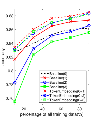
Figure 3: Tagging results. “Baseline($w$)” refers to the baseline tagger with context of $\pm w$ words; “TokenEmbedding($w$+$w^{\prime}$)” refers to the token embedding tagger with tagger context of $\pm w$ words and token embedding context of $\pm w^{\prime}$ words.

We first train our baseline tagger without the binary feature vector using different amounts of training data and window sizes $w\in\{0,1,2,3\}$. Figure 3 shows accuracies on the validation set. When using only 10% of the training data, the baseline tagger with $w=0$ performs best. As the amount of training data increases, the larger window sizes begin to outperform $w=0$, and with the full training set, $w=1$ performs best.

Figure 3 also shows the results of our token embedding tagger for $w=0$ and $w^{\prime}\in\{1,2,3\}$. We see consistent gains when using token embeddings, higher than the best baseline window for all values of $w^{\prime}$, though the best performance is obtained with $w^{\prime}=1$. When using small amounts of data, the baseline accuracy drops when increasing $w$, but the token embedding tagger is much more robust, always outperforming the $w=0$ baseline.

We then perform experiments using the full training set, showing results in Table 5. For all experiments with the baseline DNN tagger, we fix $w=1$; when using token embeddings, we fix $w=0$ and $w^{\prime}=1$. We also consider updating the initial word type embeddings during tagger training (“updating”) and using the binary feature vector for the center word (“features”).

Using token embeddings consistently outperforms using type embeddings alone. On the test set, we see gains from token embeddings across all settings, ranging from 0.5 to 1.2. The gains from DNN and seq2seq token embeddings are similar (possibly because we again use $w=0$ and $w^{\prime}=1$ for the latter). The baseline taggers improve substantially by updating type embeddings or adding features (settings (2) or (3)), but adding token embeddings still yields additional improvements. When we use token embeddings but remove the type embedding for the word being tagged (denoted “*”), DNN TEs can still improve over the baseline, though seq2seq TEs yield lower accuracy. This suggests that the seq2seq TE model is focusing on other information in the window that is not necessarily related to the center word.

	val.	test
(1) Baseline	88.4	88.9
(1) + DNN TE	+1.6	+0.9
(2) Baseline + updating	89.4	89.4
(2) + DNN TE	+0.6	+0.5
(3) Baseline + features	89.2	89.3
(3) + DNN TE*	+0.6	+0.3
(3) + DNN TE	+1.2	+1.2
(3) Baseline + features	89.2	89.3
(3) + seq2seq TE*	-0.6	-1.0
(3) + seq2seq TE	+1.3	+1.0

Table 5: Tagging accuracies (%) on validation (Oct27Test) and test (Daily547) sets. Accuracy deltas are always relative to the respective baseline in each section of the table. “updating” = updates type embeddings during training, “features” = uses binary feature vector for center word, * = omits center word type embedding.

	val.	test
(4) Baseline + all features	92.1	92.2
(4) + updating	92.2	92.4
(4) + DNN TE + without updating	92.4	92.8
Owoputi et al.	91.6	92.8

Table 6: Tagging accuracies (%) on validation (Oct27Test) and test (Daily547) sets using all features: Brown clusters, tag dictionaries, name lists, and character $n$-grams. Last row is best result from Owoputi et al. (2013).

Comparison to State of the Art.

Owoputi et al. (2013) achieve 92.8% on this train/test setup, using structured prediction and additional features from annotated and curated resources. We add several additional features inspired by theirs. We use features based on their generated Brown clusters, namely, binary vectors representing indicators for cluster string prefixes of length 2, 4, 6, and 8. We add tag dictionary features constructed from the Wall Street Journal portion of the Penn Treebank Marcus et al. (1993). We use the concatenation of the binary tag vectors for the three most common tags in the tag dictionary for the word being tagged. We use the 10-dimensional binary feature vector and a binary feature indicating whether the word begins with a capital letter. All features above are used for the center word as well as one word to the left and one word to the right.

We add several more features only for the word being tagged. We use name list features, adding a binary feature for each name list used by Owoputi et al. (2013), where the feature indicates membership on the corresponding name list of the word being tagged. We also include character $n$-gram count features for $n\in\{2,3\}$, adding features for the 3,133 bi/trigrams that appear 3 or more times in the tagging training data.

After adding these features, we increase the hidden layer size to 2048. We use dropout, using a dropout rate of 0.2 for the input layer and 0.4 for the hidden layers. The other settings remain the same. The results are shown in Table 6. Our new baseline tagger improves from 89.2% to 92.1% on validation, and improves further with updating.

We then add DNN token embeddings to this new baseline. When doing so, we set $w=0$, as in all earlier experiments. We add two sets of DNN token embedding features to the tagger, one with $w^{\prime}=1$ and another with $w^{\prime}=3$. The results improve by 0.4 over the strongest baseline on the test set, matching the accuracy of Owoputi et al. (2013). This is notable since they used structured prediction while we use a simple local classifier, enabling fast and maximally-parallelizable test-time inference.

7.2 Dependency Parsing

We show results with our head predictors in Table 7. The baseline head predictor actually does best with $w=0$. The predictors with token embeddings are able to leverage larger context: with DNN token embeddings, performance is best with $w^{\prime}=1$ while with seq2seq token embeddings, performance is strong with $w^{\prime}=1$ and 2. When using token embeddings, we actually found it beneficial to drop the center word type embedding from the input, only using it indirectly through the token embedding functions. We use $w=-1$ to indicate this setting.

The upper part of Table 8 shows the results when we simply use our parsers to output the highest-scoring parents for each word in the test set. Token embeddings are more helpful for this task than type embeddings, improving performance from 73.0 to 75.8 for DNN token embeddings and improving to 75.0 for the seq2seq token embeddings.

We also use our head predictors to add a new feature to TweeboParser Kong et al. (2014). TweeboParser uses a feature on every candidate arc corresponding to the score under a first-order dependency model trained on the Penn Treebank. We add a similar feature corresponding to the arc score under our model from our head predictors. Because TweeboParser results are nondeterministic, presumably due to floating point precision, we train TweeboParser 10 times for both its baseline configuration and all settings using our additional features, using TweeboParser’s default hyperparameters each time. We report means and standard deviations.

The final results are shown in the lower part of Table 8. While adding the feature from the baseline parser hurts performance slightly (80.6$\rightarrow$ 80.5), adding token embeddings improves performance. Using the feature from our DNN TE head predictor improves performance to 81.5, establishing a new state of the art for Twitter dependency parsing.

$w$ or $w^{\prime}$	Baseline	DNN TE	seq2seq TE
0	75.8	-	-
1	75.4	77.8	77.8
2	73.2	77.3	77.9
3	72.3	77.2	76.9

Table 7: Attachment $F_{1}$ (%) on validation set using different models and window sizes. For TE columns, the input does not include any type embeddings at all, only token embeddings. Best result in each column is in boldface.

(1) Baseline parser ($w=0$)	73.0
(1) + DNN TE ($w=-1,w^{\prime}=1$)	75.8
(1) + seq2seq TE ($w=-1,w^{\prime}=1$)	75.0
(1) + seq2seq TE ($w=-1,w^{\prime}=2$)	74.2
(2) Kong et al.	80.6 $\pm$ 0.25
(2) + Baseline parser ($w=0$)	80.5 $\pm$ 0.30
(2) + DNN TE ($w=-1,w^{\prime}=1$)	81.5 $\pm$ 0.25
(2) + seq2seq TE ($w=-1,w^{\prime}=1$)	81.0 $\pm$ 0.17
(2) + seq2seq TE ($w=-1,w^{\prime}=2$)	80.9 $\pm$ 0.33

Table 8: Dependency parsing unlabeled attachment $F_{1}$ (%) on test (Test-New) sets for baseline parser and results when augmented with token embedding features. Following Kong et al., we report three significant digits.

8 Conclusion

We have presented a simple and efficient way of learning representations of words in their contexts using unlabeled data, and have shown how they can be used to improve syntactic analysis of Twitter. Qualitatively, our token embeddings are shown to encode sense and POS information, grouping together tokens of different types with similar in-context meanings. Quantitatively, using token embeddings in simple predictors consistently improves performance, even rivaling the performance of strong structured prediction baselines. Our code and trained token embedding models are publicly available at the authors’ websites. Future work includes further exploration of token embedding models, unsupervised objectives, and their integration with supervised predictors.

References

- Bansal et al. (2014) Mohit Bansal, Kevin Gimpel, and Karen Livescu. 2014. Tailoring continuous word representations for dependency parsing. In Proc. of ACL.
- Chen et al. (2014) Xinxiong Chen, Zhiyuan Liu, and Maosong Sun. 2014. A unified model for word sense representation and disambiguation. In Proc. of EMNLP.
- Choi et al. (2016) Heeyoul Choi, Kyunghyun Cho, and Yoshua Bengio. 2016. Context-dependent word representation for neural machine translation. arXiv preprint arXiv:1607.00578 .
- Clark and Araki (2011) Eleanor Clark and Kenji Araki. 2011. Text normalization in social media: progress, problems and applications for a pre-processing system of casual English. Procedia-Social and Behavioral Sciences 27.
- Collobert et al. (2011) Ronan Collobert, Jason Weston, Léon Bottou, Michael Karlen, Koray Kavukcuoglu, and Pavel Kuksa. 2011. Natural language processing (almost) from scratch. Journal of Machine Learning Research 12.
- Dai and Le (2015) Andrew M. Dai and Quoc V. Le. 2015. Semi-supervised sequence learning. In Advances in NIPS.
- Dieleman et al. (2015) Sander Dieleman, Jan Schlüter, Colin Raffel, Eben Olson, Søren Kaae Sønderby, Daniel Nouri, Daniel Maturana, Martin Thoma, Eric Battenberg, Jack Kelly, et al. 2015. Lasagne: First release. http://dx.doi.org/10.5281/zenodo.27878.
- Gers et al. (2000) Felix A. Gers, Jürgen Schmidhuber, and Fred Cummins. 2000. Learning to forget: Continual prediction with LSTM. Neural Computation 12(10).
- Gimpel et al. (2011) Kevin Gimpel, Nathan Schneider, Brendan O’Connor, Dipanjan Das, Daniel Mills, Jacob Eisenstein, Michael Heilman, Dani Yogatama, Jeffrey Flanigan, and Noah A. Smith. 2011. Part-of-speech tagging for Twitter: annotation, features, and experiments. In Proc. of ACL.
- Gonen and Goldberg (2016) Hila Gonen and Yoav Goldberg. 2016. Semi supervised preposition-sense disambiguation using multilingual data. In Proc. of COLING.
- Graves et al. (2013) Alan Graves, Abdel-rahman Mohamed, and Geoffrey Hinton. 2013. Speech recognition with deep recurrent neural networks. In Proc. of ICASSP.
- Guo et al. (2014) Jiang Guo, Wanxiang Che, Haifeng Wang, and Ting Liu. 2014. Learning sense-specific word embeddings by exploiting bilingual resources. In Proc. of COLING.
- Hochreiter and Schmidhuber (1997) Sepp Hochreiter and Jürgen Schmidhuber. 1997. Long short-term memory. Neural Computation 9(8).
- Huang et al. (2012) Eric Huang, Richard Socher, Christopher D. Manning, and Andrew Ng. 2012. Improving word representations via global context and multiple word prototypes. In Proc. of ACL.
- Jauhar et al. (2015) Sujay Kumar Jauhar, Chris Dyer, and Eduard Hovy. 2015. Ontologically grounded multi-sense representation learning for semantic vector space models. In Proc. of NAACL-HLT.
- Kågebäck et al. (2015) Mikael Kågebäck, Fredrik Johansson, Richard Johansson, and Devdatt Dubhashi. 2015. Neural context embeddings for automatic discovery of word senses. In Proc. of NAACL-HLT.
- Kawakami and Dyer (2015) Kazuya Kawakami and Chris Dyer. 2015. Learning to represent words in context with multilingual supervision. In Proc. of ICLR Workshop.
- Kong et al. (2014) Lingpeng Kong, Nathan Schneider, Swabha Swayamdipta, Archna Bhatia, Chris Dyer, and Noah A. Smith. 2014. A dependency parser for tweets. In Proc. of EMNLP.
- Li and Jurafsky (2015) Jiwei Li and Dan Jurafsky. 2015. Do multi-sense embeddings improve natural language understanding? In Proc. of EMNLP.
- Li et al. (2015) Jiwei Li, Thang Luong, and Dan Jurafsky. 2015. A hierarchical neural autoencoder for paragraphs and documents. In Proc. of ACL.
- Ling et al. (2015) Wang Ling, Chris Dyer, Alan W. Black, Isabel Trancoso, Ramon Fermandez, Silvio Amir, Luis Marujo, and Tiago Luis. 2015. Finding function in form: Compositional character models for open vocabulary word representation. In Proc. of EMNLP.
- Liu et al. (2015) Yang Liu, Zhiyuan Liu, Tat-Seng Chua, and Maosong Sun. 2015. Topical word embeddings. In Proc. of AAAI.
- Maaten and Hinton (2008) Laurens van der Maaten and Geoffrey Hinton. 2008. Visualizing data using t-SNE. Journal of Machine Learning Research 9.
- Marcus et al. (1993) Mitchell P. Marcus, Mary Ann Marcinkiewicz, and Beatrice Santorini. 1993. Building a large annotated corpus of English: The Penn Treebank. Computational Linguistics 19(2).
- Melamud et al. (2016) Oren Melamud, Jacob Goldberger, and Ido Dagan. 2016. context2vec: Learning generic context embedding with bidirectional LSTM. In Proc. of CoNLL.
- Mikolov et al. (2013) Tomas Mikolov, Ilya Sutskever, Kai Chen, Greg S. Corrado, and Jeff Dean. 2013. Distributed representations of words and phrases and their compositionality. In Advances in NIPS.
- Neelakantan et al. (2014) Arvind Neelakantan, Jeevan Shankar, Alexandre Passos, and Andrew McCallum. 2014. Efficient non-parametric estimation of multiple embeddings per word in vector space. In Proc. of EMNLP.
- Owoputi et al. (2013) Olutobi Owoputi, Brendan O’Connor, Chris Dyer, Kevin Gimpel, Nathan Schneider, and Noah A. Smith. 2013. Improved part-of-speech tagging for online conversational text with word clusters. In Proc. of NAACL.
- Pennington et al. (2014) Jeffrey Pennington, Richard Socher, and Christopher D. Manning. 2014. GloVe: Global vectors for word representation. In Proc. of EMNLP.
- Peters et al. (2017) Matthew E. Peters, Waleed Ammar, Chandra Bhagavatula, and Russell Power. 2017. Semi-supervised sequence tagging with bidirectional language models. In Proc. of ACL.
- Piña and Johansson (2015) Luis Nieto Piña and Richard Johansson. 2015. A simple and efficient method to generate word sense representations. In Proc. of RANLP.
- Qiu et al. (2014) Lin Qiu, Yong Cao, Zaiqing Nie, and Yong Rui. 2014. Learning word representation considering proximity and ambiguity. In Proc. of AAAI.
- Reisinger and Mooney (2010) Joseph Reisinger and Raymond J. Mooney. 2010. Multi-prototype vector-space models of word meaning. In Proc. of NAACL.
- Sundermeyer et al. (2012) Martin Sundermeyer, Ralf Schlüter, and Hermann Ney. 2012. LSTM neural networks for language modeling. In Proc. of Interspeech.
- Šuster et al. (2016) Simon Šuster, Ivan Titov, and Gertjan van Noord. 2016. Bilingual learning of multi-sense embeddings with discrete autoencoders. In Proc. of NAACL.
- Sutskever et al. (2014) Ilya Sutskever, Oriol Vinyals, and Quoc V. Le. 2014. Sequence to sequence learning with neural networks. In Advances in NIPS.
- Theano Development Team (2016) Theano Development Team. 2016. Theano: A Python framework for fast computation of mathematical expressions. arXiv e-prints abs/1605.02688.
- Tian et al. (2014) Fei Tian, Hanjun Dai, Jiang Bian, Bin Gao, Rui Zhang, Enhong Chen, and Tie-Yan Liu. 2014. A probabilistic model for learning multi-prototype word embeddings. In Proc. of COLING.
- Turian et al. (2010) Joseph Turian, Lev Ratinov, and Yoshua Bengio. 2010. Word representations: a simple and general method for semisupervised learning. In Proc. of ACL.
- Vu and Parker (2016) Thuy Vu and D. Stott Parker. 2016. -embeddings: Learning conceptual embeddings for words using context. In Proc. of NAACL-HLT.
- Wu and Giles (2015) Zhaohui Wu and C. Lee Giles. 2015. Sense-aware semantic analysis: A multi-prototype word representation model using Wikipedia. In Proc. of AAAI.
- Zou et al. (2013) Will Y. Zou, Richard Socher, Daniel Cer, and Christopher D. Manning. 2013. Bilingual word embeddings for phrase-based machine translation. In Proc. of EMNLP.