The FastMap Algorithm for Shortest Path Computations

Abstract

We present a new preprocessing algorithm for embedding the nodes of a given edge-weighted undirected graph into a Euclidean space. The Euclidean distance between any two nodes in this space approximates the length of the shortest path between them in the given graph. Later, at runtime, a shortest path between any two nodes can be computed with A* search using the Euclidean distances as heuristic. Our preprocessing algorithm, called FastMap, is inspired by the data mining algorithm of the same name and runs in near-linear time. Hence, FastMap is orders of magnitude faster than competing approaches that produce a Euclidean embedding using Semidefinite Programming. FastMap also produces admissible and consistent heuristics and therefore guarantees the generation of shortest paths. Moreover, FastMap applies to general undirected graphs for which many traditional heuristics, such as the Manhattan Distance heuristic, are not well defined. Empirically, we demonstrate that A* search using the FastMap heuristic is competitive with A* search using other state-of-the-art heuristics, such as the Differential heuristic.

Introduction and Related Work

Shortest path computations commonly occur in the inner procedures of many AI programs. In video games, for example, a large fraction of CPU cycles is spent on shortest path computations Uras and Koenig (2015). Many other tasks in AI, including motion planning LaValle (2006), temporal reasoning Dechter (2003), and decision making Russell and Norvig (2009), also involve finding and reasoning about shortest paths. While Dijkstra’s algorithm Dijkstra (1959) can be used to compute shortest paths in polynomial time, speeding up shortest path computations allows one to solve the aformentioned tasks faster. One way to do that is to use A* search with an informed heuristic Hart et al. (1968).

A perfect heuristic is one that returns the true distance between any two nodes in a given graph. A* with such a heuristic and proper tie-breaking is guaranteed to expand nodes only on a shortest path between the given start and goal nodes. In general, computing the perfect heuristic between two nodes is as hard as computing the shortest path between them. Hence, A* search benefits from a perfect heuristic only if it is computed offline. However, precomputing all pairwise distances is not only time-intensive but also requires a prohibitive $O(N^{2})$ memory where $N$ is the number of nodes. The memory requirements for storing all-pairs shortest paths data can be somewhat addressed through compression Botea and Harabor (2013); Strasser et al. (2015).

Existing methods for preprocessing a given graph (without precomputing all pairwise distances) can be grouped into the following categories: Hierarchical abstractions that yield suboptimal paths have been used to reduce the size of the search space by abstracting groups of nodes Botea et al. (2004); Sturtevant and Buro (2005). More informed heuristics Björnsson and Halldórsson (2006); Cazenave (2006); Sturtevant et al. (2009) focus A* searches better, resulting in fewer expanded states. Hierarchies can also be used to derive heuristics during the search Leighton et al. (2008); Holte et al. (1994). Dead-end detection and other pruning methods Björnsson and Halldórsson (2006); Goldenberg et al. (2010); Pochter et al. (2010) identify areas of the graph that do not need to be searched to find shortest paths. Search with contraction hierarchies Geisberger et al. (2008) is an optimal hierarchical method, where every level of the hierarchy contains only a single node. It has been shown to be efficient on road networks but seems to be less efficient on graphs with higher branching factors, such as grid-based game maps Storandt (2013). N-level graphs Uras and Koenig (2014), constructed from undirected graphs by partitioning the nodes into levels also allow for significant pruning during the search.

A different approach that does not rely on preprocessing of the graph is to use some notion of a geometric distance between two nodes as a heuristic of the distance between them. One such heuristic for gridworlds is the Manhattan Distance heuristic. For many gridworlds, A* search using the Manhattan Distance heuristic outperforms Dijkstra’s algorithm. However, in complicated 2D/3D gridworlds like mazes, the Manhattan Distance heuristic may not be sufficiently informed to focus A* searches effectively. Another issue associated with Manhattan Distance-like heuristics is that they are not well defined for general graphs. For a graph that cannot be conceived in a geometric space, there is no closed-form formula for a “geometric” heuristic for the distance between two nodes because there are no coordinates associated with them.

For a graph that does not already have a geometric embedding in Euclidean space, a preprocessing algorithm can be used to generate one. As described before, at runtime, A* search would then use the Euclidean distance between any two nodes in this space as an estimate for the distance between them in the given graph. One such approach is Euclidean Heuristic Optimization (EHO) Rayner et al. (2011). EHO guarantees admissiblility and consistency and therefore generates shortest paths. However, it requires solving a Semidefinite Program (SDP). SDPs can be solved in polynomial time Vandenberghe and Boyd (1996). EHO leverages additional structure to solve them in cubic time. Still, a cubic preprocessing time limits the size of the graphs that are amenable to this approach.

The Differential heuristic is another state-of-the-art approach that has the benefit of a near-linear runtime. However, unlike the approach in Rayner et al. (2011), it does not produce an explicit Euclidean embedding. In the preprocessing phase of the Differential heuristic approach, some nodes of the graph are chosen as pivot nodes. The distances between each pivot node and every other node are precomputed and stored Sturtevant et al. (2009). At runtime, the heuristic between two nodes $a$ and $b$ is given by $\max_{p}|d(a,p)-d(p,b)|$, where $p$ is a pivot node and $d(\cdot,\cdot)$ is the precomputed distance. The preprocessing time is linear in the number of pivots times the size of the graph. The required space is linear in the number of pivots times the number of nodes, although a more succinct representation is presented in Goldenberg et al. (2011). Similar preprocessing techniques are used in Portal-Based True Distance heuristics Goldenberg et al. (2010).

In this paper, we present a new preprocessing algorithm, called FastMap, that produces an explicit Euclidean embedding while running in near-linear time. It therefore has the benefits of the small preprocessing time of the Differential heuristic approach and of producing an embedding from which a heuristic between two nodes can be quickly computed using a closed-form formula. Our preprocessing algorithm, dubbed FastMap, is inspired by the data mining algorithm of the same name Faloutsos and Lin (1995). It is orders of magnitude faster than SDP-based approaches for producing Euclidean embeddings. FastMap also produces admissible and consistent heuristics and therefore guarantees the generation of shortest paths.

The FastMap heuristic has several advantages: First, it is defined for general (undirected) graphs. Second, we observe empirically that, in gridworlds, A* using the FastMap heuristic runs faster than A* using the Manhattan or Octile distance heuristics. A* using the FastMap heuristic runs equally fast or faster than A* using the Differential heuristic, with the same memory resources. The (explicit) Euclidean embedding produced by FastMap also has representational benefits like recovering the underlying manifolds of the graph and/or visualizing them. Moreover, we observe that the FastMap and Differential heuristics have complementary strengths and can be easily combined to generate an even more informed heuristic.

The Origin of FastMap

The FastMap algorithm Faloutsos and Lin (1995) was introduced in the data mining community for automatically generating geometric embeddings of abstract objects. For example, if we are given objects in form of long DNA strings, multimedia datasets such as voice excerpts or images, or medical datasets such as ECGs or MRIs, there is no geometric space in which these objects can be naturally visualized. However, there is often a well defined distance function between every pair of objects. For example, the edit distance between two DNA strings is well defined although an individual DNA string cannot be conceptualized in geometric space.

Clustering techniques, such as the $k$-means algorithm, are well studied in machine learning Alpaydin (2010) but cannot be applied directly to domains with abstract objects because they assume that objects are described as points in geometric space. FastMap revives their applicability by first creating a Euclidean embedding for the abstract objects that approximately preserves the pairwise distances between them. Such an embedding also helps to visualize the abstract objects, for example, to aid physicians in identifying correlations between symptoms from medical records.

The data mining FastMap gets as input a complete undirected edge-weighted graph $G=(V,E)$. Each node $v_{i}\in V$ represents an abstract object $O_{i}$. Between any two nodes $v_{i}$ and $v_{j}$ there is an edge $(v_{i},v_{j})\in E$ with weight $D(O_{i},O_{j})$ that corresponds to the given distance between objects $O_{i}$ and $O_{j}$. A Euclidean embedding assigns to each object $O_{i}$ a $K$-dimensional point $p_{i}\in\mathbb{R}^{K}$. A good Euclidean embedding is one in which the Euclidean distance between any two points $p_{i}$ and $p_{j}$ closely approximates $D(O_{i},O_{j})$.

One of the early approaches for generating such an embedding is based on the idea of multi-dimensional scaling (MDS) Torgerson (1952). Here, the overall distortion of the pairwise distances is measured in terms of the “energy” stored in “springs” that connect each pair of objects. MDS, however, requires $O(|V|^{2})$ time and hence does not scale well in practice. On the other hand, FastMap Faloutsos and Lin (1995) requires only linear time. Both methods embed the objects in a $K$-dimensional space for a user-specified $K$.

FastMap works as follows: In the very first iteration, it heuristically identifies the farthest pair of objects $O_{a}$ and $O_{b}$ in linear time. It does this by initially choosing a random object $O_{b}$ and then choosing $O_{a}$ to be the farthest object away from $O_{b}$. It then reassigns $O_{b}$ to be the farthest object away from $O_{a}$. Once $O_{a}$ and $O_{b}$ are determined, every other object $O_{i}$ defines a triangle with sides of lengths $d_{ai}=D(O_{a},O_{i})$, $d_{ab}=D(O_{a},O_{b})$ and $d_{ib}=D(O_{i},O_{b})$. Figure 1 shows this triangle. The sides of the triangle define its entire geometry, and the projection of $O_{i}$ onto $O_{a}O_{b}$ is given by $x_{i}=(d_{ai}^{2}+d_{ab}^{2}-d_{ib}^{2})/(2d_{ab})$. FastMap sets the first coordinate of $p_{i}$, the embedding of object $O_{i}$, to $x_{i}$. In particular, the first coordinate of $p_{a}$ is $x_{a}=0$ and of $p_{b}$ is $x_{b}=d_{ab}$. Computing the first coordinates of all objects takes only linear time since the distance between any two objects $O_{i}$ and $O_{j}$ for $i,j\notin\{a,b\}$ is never computed.

Figure 1: The three sides of a triangle define its entire geometry. In particular, $x_{i}=(d_{ai}^{2}+d_{ab}^{2}-d_{ib}^{2})/(2d_{ab})$.

In the subsequent $K-1$ iterations, the same procedure is followed for computing the remaining $K-1$ coordinates of each object. However, the distance function is adapted for different iterations. For example, for the first iteration, the coordinates of $O_{a}$ and $O_{b}$ are $0$ and $d_{ab}$, respectively. Because these coordinates fully explain the true distance between them, from the second iteration onwards, the rest of $p_{a}$ and $p_{b}$’s coordinates should be identical. Intuitively, this means that the second iteration should mimic the first one on a hyperplane that is perpendicular to the line $O_{a}O_{b}$. Figure 2 explains this intuition. Although the hyperplane is never constructed explicitly, its conceptualization implies that the distance function for the second iteration should be changed in the following way: $D_{new}(O^{\prime}_{i},O^{\prime}_{j})^{2}=D(O_{i},O_{j})^{2}-(x_{i}-x_{j})^{2}$. Here, $O^{\prime}_{i}$ and $O^{\prime}_{j}$ are the projections of $O_{i}$ and $O_{j}$, respectively, onto this hyperplane, and $D_{new}$ is the new distance function.

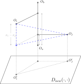
Figure 2: Shows a geometric conceptualization of the recursive step in FastMap. In particular, $D_{new}(O^{\prime}_{i},O^{\prime}_{j})^{2}=D(O_{i},O_{j})^{2}-(x_{i}-x_{j})^{2}$.

FastMap for Shortest Path Computations

In this section, we provide the high-level ideas for how to adapt the data mining FastMap algorithm to shortest path computations. In the shortest path computation problem, we are given a non-negative edge-weighted undirected graph $G=(V,E)$ along with a start node $v_{s}$ and a goal node $v_{g}$. As a preprocessing technique, we can embed the nodes of $G$ in a Euclidean space. As A* searches for a shortest path from $v_{s}$ to $v_{g}$, it can use the Euclidean distance from $v\in V$ to $v_{g}$ as a heuristic for $v$. The number of node expansions of A* search depends on the informedness of the heuristic which, in turn, depends on the ability of the embedding to preserve the pairwise distances.

The idea is to view the nodes of $G$ as the objects to be embedded in Euclidean space. As such, the data mining FastMap algorithm cannot directly be used for generating an embedding in linear time. The data mining FastMap algorithm assumes that the distance $d_{ij}$ between two objects $O_{i}$ and $O_{j}$ can be computed in constant time, independent of the number of objects. Computing the distance between two nodes depends on the size of the graph. Another problem is that the Euclidean distances may not satisfy important properties such as admissibility or consistency. Admissibility guarantees that A* finds shortest paths while consistency allows A* to avoid re-expansions of nodes as well.

The first issue of having to retain (near-)linear time complexity can be addressed as follows: In each iteration, after we identify the farthest pair of nodes $O_{a}$ and $O_{b}$, the distances $d_{ai}$ and $d_{ib}$ need to be computed for all other nodes $O_{i}$. Computing $d_{ai}$ and $d_{ib}$ for any single node $O_{i}$ can no longer be done in constant time but requires $O(|E|+|V|\log|V|)$ time instead Fredman and Tarjan (1984). However, since we need to compute these distances for all nodes, computing two shortest path trees rooted at nodes $O_{a}$ and $O_{b}$ yields all necessary distances. The complexity of doing so is also $O(|E|+|V|\log|V|)$, which is only linear in the size of the graph. The amortized complexity for computing $d_{ai}$ and $d_{ib}$ for any single node $O_{i}$ is therefore near-constant time.

The second issue of having to generate a consistent (and thus admissible) heuristic is formally addressed in Theorem 1. The idea is to use $L_{1}$ distances instead of $L_{2}$ distances in each iteration of FastMap. The mathematical properties of the $L_{1}$ distance can be used to prove that admissibility and consistency hold irrespective of the dimensionality of the embedding.

Input: $G=(V,E,w)$, $K_{max}$ and $\epsilon$.

Output: $K$ and $p_{i}\in\mathbb{R}^{K}$ for all $v_{i}\in V$.

1 $w^{\prime}=w$; $\ \ K=1$;

2 while $K_{max}>0$ do

3       Let $G^{\prime}=(V,E,w^{\prime})$;

4       $(n_{a},n_{b})\leftarrow$ GetFarthestPair($G^{\prime}$);

5       Compute shortest path trees rooted at $n_{a}$ and $n_{b}$ on $G^{\prime}$ to obtain $d_{ab}$, $d_{ai}$ and $d_{ib}$ for all $v_{i}\in V$;

6       if $d_{ab}<\epsilon$ then

7             Break;

8            

9      for each $v\in V$ do

10             $[p_{v}]_{K}=(d_{av}+d_{ab}-d_{vb})/2$

11      for each edge $(u,v)\in E$ do

12             $w^{\prime}(u,v)=w^{\prime}(u,v)-|[p_{u}]_{K}-[p_{v}]_{K}|$;

13            

14      $K=K+1$; $\ \ K_{max}=K_{max}-1$;

15      

Algorithm 1 Shows the FastMap algorithm. $G=(V,E,w)$ is a non-negative edge-weighted undirected graph; $K_{max}$ is the user-specified upper bound on the dimensionality; $\epsilon$ is a user-specified threshold; $K\leq K_{max}$ is the dimensionality of the computed embedding; $p_{i}$ is the Euclidean embedding of node $v_{i}\in V$. Line $11$ is equivalent to $w^{\prime}(u,v)=w(u,v)-\lVert p_{u}-p_{v}\rVert_{1}$.

Algorithm 1 presents data mining FastMap adapted to the shortest path computation problem. The input is an edge-weighted undirected graph $G=(V,E,w)$ along with two user-specified parameters $K_{max}$ and $\epsilon$. $K_{max}$ is the maximum number of dimensions allowed in the Euclidean embedding. It bounds the amount of memory needed to store the Euclidean embedding of any node. $\epsilon$ is the threshold that marks a point of diminishing returns when the distance between the farthest pair of nodes becomes negligible. The output is an embedding $p_{i}\in\mathbb{R}^{K}$ (with $K\leq K_{max}$) for each node $v_{i}\in V$.

The algorithm maintains a working graph $G^{\prime}=(V,E,w^{\prime})$ initialized to $G$. The nodes and edges of $G^{\prime}$ are always identical to those of $G$ but the weights on the edges of $G^{\prime}$ change with every iteration. In each iteration, the farthest pair ($n_{a},n_{b}$) of nodes in $G^{\prime}$ is heuristically identified in near-linear time (line $4$). The $K^{th}$ coordinate $[p_{i}]_{K}$ of each node $v_{i}$ is computed using a formula similar to that for $x_{i}$ in Figure 1. However, that formula is modified to $(d_{ai}+d_{ab}-d_{ib})/2$ to ensure admissibility and consistency of the heuristic. In each iteration, the weight of each edge is decremented to resemble the update rule for $D_{new}$ in Figure 2 (line $11$). However, that update rule is modified to $w^{\prime}(u,v)=w^{\prime}(u,v)-|[p_{u}]_{K}-[p_{v}]_{K}|$ to use the $L_{1}$ distances instead of the $L_{2}$ distances.

The method GetFarthestPair($G^{\prime}$) (line $4$) computes shortest path trees in $G^{\prime}$ a small constant number of times, denoted by $\tau$. It therefore runs in near-linear time. In the first iteration, we assign $n_{a}$ to be a random node. A shortest path tree rooted at $n_{a}$ is computed to identify the farthest node from it. $n_{b}$ is assigned to be this farthest node. In the next iteration, a shortest path tree rooted at $n_{b}$ is computed to identify the farthest node from it. $n_{a}$ is reassigned to be this farthest node. Subsequent iterations follow the same switching rule for $n_{a}$ and $n_{b}$. The final assignments of nodes to $n_{a}$ and $n_{b}$ are returned after $\tau$ iterations. This entire process of starting from a randomly chosen node can be repeated a small constant number of times.

Figure 3 shows the working of our algorithm on a small gridworld example.

(a)

(b)

(c)

(d)

(e)

(f)

(g)

(h)

(i)

(j)

Figure 3: Illustrates the working of FastMap. (a) shows a $4$-neighbor gridworld with obstacles in black. (b) shows the graphical representation of (a) with the original unit weights on the edges. (c) shows the identified farthest pair of nodes. (d) shows two numbers in each cell representing the distances from $n_{a}$ and $n_{b}$, respectively. (e) shows the first coordinate produced for each cell. (f) shows new edge weights for the next iteration. (g), (h) and (i) correspond to (c), (d) and (e), respectively, in the second iteration. (j) shows the produced $2$D embedding.

Proof of Consistency

In this section, we prove the consistency of the FastMap heuristic. Since consistency implies admissibility, this also proves that A* with the FastMap heuristic returns shortest paths. We use the following notation in the proofs: $w^{i}_{xy}$ is the weight on the edge between nodes $x$ and $y$ in the $i^{th}$ iteration; $d^{i}_{xy}$ is the distance between nodes $x$ and $y$ in the $i^{th}$ iteration (using the weights $w^{i}$); $p_{x}$ is the vector of coordinates produced for node $x$, and $[p_{x}]_{j}$ is its $j^{th}$ coordinate; $h^{i}_{xy}$ is the FastMap heuristic between nodes $x$ and $y$ after $i$ iterations. Note that $h^{i}_{xy}$ is the $L_{1}$ distance between $p_{x}$ and $p_{y}$ at iteration $i$, that is $h^{i}_{xy}\vcentcolon=\sum_{j=1}^{i}|[p_{x}]_{j}-[p_{y}]_{j}|$. We also define $\Delta^{i+1}_{xy}\vcentcolon=d^{i}_{xy}-d^{i+1}_{xy}$. In the following proofs, we use the fact that $|A|+|B|\geq|A+B|$ and $|A|-|B|\leq|A-B|$.

Lemma 1.

For all $x$, $y$ and $i$, $d^{i}_{xy}\geq 0$.

Proof.

We prove by induction that in any iteration $i$, $w^{i}_{uv}\geq 0$ for all $(u,v)\in E$. Thus, the weight of each edge in the $i^{th}$ iteration is non-negative and therefore $d^{i}_{uv}\geq 0$ for all $u$, $v$. For the base case, $w^{1}_{uv}=w(u,v)\geq 0$. We assume that $w^{i}_{uv}\geq 0$ and show that $w^{i+1}_{uv}\geq 0$. Let $n_{a}$ and $n_{b}$ be the farthest pair of nodes identified in the $i^{th}$ iteration. From lines $9$ and $11$, $w^{i+1}_{uv}=w^{i}_{uv}-|(d^{i}_{au}-d^{i}_{av})/2+(d^{i}_{vb}-d^{i}_{ub})/2|$. To show that $w^{i+1}_{uv}\geq 0$ we show that $w^{i}_{uv}\geq|(d^{i}_{au}-d^{i}_{av})/2+(d^{i}_{vb}-d^{i}_{ub})/2|$. From the triangle inequality, for any node $l$, $d^{i}_{uv}+\min(d^{i}_{ul},d^{i}_{lv})\geq\max(d^{i}_{ul},d^{i}_{lv})$. Therefore, $d^{i}_{uv}\geq|d^{i}_{lv}-d^{i}_{ul}|$. This means that $d^{i}_{uv}\geq|d^{i}_{au}-d^{i}_{av}|/2+|d^{i}_{vb}-d^{i}_{ub}|/2$. Therefore, $d^{i}_{uv}\geq|(d^{i}_{au}-d^{i}_{av})/2+(d^{i}_{vb}-d^{i}_{ub})/2|$. This concludes the proof since $w^{i}_{uv}\geq d^{i}_{uv}$. ∎

Lemma 2.

For all $x$, $y$ and $i$, $\Delta^{i+1}_{xy}\geq|[p_{x}]_{i}-[p_{y}]_{i}|$.

Proof.

Let $\langle u_{1}=x,\ldots,u_{m}=y\rangle$ be the shortest path from $x$ to $y$ in iteration $i$. By definition, $d^{i}_{xy}=\sum_{j=1}^{m-1}w^{i}_{u_{j}u_{j+1}}$ and $d^{i+1}_{xy}\leq\sum_{j=1}^{m-1}w^{i+1}_{u_{j}u_{j+1}}$. From line $11$, $w^{i+1}_{u_{j}u_{j+1}}=w^{i}_{u_{j}u_{j+1}}-|[p_{u_{j}}]_{i}-[p_{u_{j+1}}]_{i}|$. Therefore, $\Delta^{i+1}_{xy}=d^{i}_{xy}-d^{i+1}_{xy}\geq\sum_{j=1}^{m-1}|[p_{u_{j}}]_{i}-[p_{u_{j+1}}]_{i}|$. This concludes the proof since $\sum_{j=1}^{m-1}|[p_{u_{j}}]_{i}-[p_{u_{j+1}}]_{i}|\geq|\sum_{j=1}^{m-1}[p_{u_{j}}]_{i}-[p_{u_{j+1}}]_{i}|=|[p_{x}]_{i}-[p_{y}]_{i}|$. ∎

Lemma 3.

For all $x$, $y$, $g$ and $i$, $d^{1}_{xy}+h^{i}_{yg}-h^{i}_{xg}\geq d^{i+1}_{xy}$.

Proof.

We prove the lemma by induction on $i$. The base case for $i=1$ is implied by Lemma $2$. We assume that $d^{1}_{xy}+h^{i}_{yg}-h^{i}_{xg}\geq d^{i+1}_{xy}$ and show $d^{1}_{xy}+h^{i+1}_{yg}-h^{i+1}_{xg}\geq d^{i+2}_{xy}$. We know that $h^{i+1}_{yg}-h^{i+1}_{xg}=h^{i}_{yg}-h^{i}_{xg}-(|[p_{x}]_{i+1}-[p_{g}]_{i+1}|-|[p_{y}]_{i+1}-[p_{g}]_{i+1}|)$. Since $|[p_{x}]_{i+1}-[p_{g}]_{i+1}|-|[p_{y}]_{i+1}-[p_{g}]_{i+1}|\leq|[p_{x}]_{i+1}-[p_{y}]_{i+1}|$, we have $h^{i+1}_{yg}-h^{i+1}_{xg}\geq h^{i}_{yg}-h^{i}_{xg}-|[p_{x}]_{i+1}-[p_{y}]_{i+1}|$. Hence, $d^{1}_{xy}+h^{i+1}_{yg}-h^{i+1}_{xg}\geq(d^{1}_{xy}+h^{i}_{yg}-h^{i}_{xg})-|[p_{x}]_{i+1}-[p_{y}]_{i+1}|$. Using the inductive assumption, we get $d^{1}_{xy}+h^{i+1}_{yg}-h^{i+1}_{xg}\geq d^{i+1}_{xy}-|[p_{x}]_{i+1}-[p_{y}]_{i+1}|$. By definition, $d_{xy}^{i+1}=\Delta_{xy}^{i+2}+d_{xy}^{i+2}$. Substituting for $d_{xy}^{i+1}$, we get $d^{1}_{xy}+h^{i+1}_{yg}-h^{i+1}_{xg}\geq d_{xy}^{i+2}+(\Delta_{xy}^{i+2}-|[p_{x}]_{i+1}-[p_{y}]_{i+1}|)$. Lemma $2$ shows that $\Delta_{xy}^{i+2}\geq|[p_{x}]_{i+1}-[p_{y}]_{i+1}|$, which concludes the proof. ∎

Theorem 1.

The FastMap heuristic is consistent.

Proof.

For all $x$, $y$, $g$ and $i$: From Lemma $3$, we know $d^{1}_{xy}+h^{i}_{yg}-h^{i}_{xg}\geq d^{i+1}_{xy}$. From Lemma $1$, we know $d^{i+1}_{xy}\geq 0$. Put together, we have $d^{1}_{xy}+h^{i}_{yg}\geq h^{i}_{xg}$. Finally, $h^{i}_{gg}=\sum_{j=1}^{i}|[p_{g}]_{j}-[p_{g}]_{j}|=0$. ∎

Theorem 2.

The informedness of the FastMap heuristic increases monotonically with the number of dimensions.

Proof.

This theorem follows from the fact that for any two nodes $x$ and $g$, $h^{i+1}_{xg}=h^{i}_{xg}+|[p_{x}]_{i+1}-[p_{g}]_{i+1}|\geq h^{i}_{xg}$. ∎

Experimental Results

We performed experiments on many benchmark maps from Sturtevant (2012). Figure 4 presents representative results. The FastMap heuristic (FM) and the Differential heuristic (DH) with equal memory resources are compared against each other. In addition, we include the Octile heuristic (OCT) as a baseline, that also uses a closed-form formula for the computation of its heuristic.

We observe that, as the number of dimensions increases, (a) FM and DH perform better than OCT; (b) the median number of expanded nodes when using the FM heuristic decreases (which is consistent with Theorem 2); and (c) the median absolute deviation (MAD) of the number of expanded nodes when using the FM heuristic decreases. When FM’s MADs are high, the variabilities can possibly be exploited in future work using Rapid Randomized Restart strategies.

FastMap also gives us a framework of identifying a point of diminishing returns with increasing dimensionality. This happens when the distance between the farthest pair of nodes stops being “significant”. For example, such a point is observed in Figure 4(f) around dimensionality $5$.

In mazes, such as in Figure 4(g), A* using the DH heuristic outperforms A* using the FM heuristic. This leads us to believe that FM provides good heuristic guidance in domains that can be approximated with a low-dimensional manifold. This observation also motivates us to create a hybrid FM+DH heuristic by taking the maximum of the two heuristics. Some relevant results are shown in Table 1. We use FM($K$) to denote the FM heuristic with $K$ dimensions and DM($K$) to denote the DH heuristic with $K$ pivots. For the results in Table 1, all heuristics have equal memory resources. We observe that the number of node expansions of A* using the FM($5$)+DH($5$) heuristic is always second best compared to A* using the FM($10$) heuristic and A* using the DH($10$) heuristic. On one hand, this decreases the percentages of instances on which it expands the least number of nodes (as seen in the second row of Table 1). But, on the other hand, its median number of node expansions is not far from that of the best technique in each breakdown.

Map	‘lak503d’						‘brc300d’						‘maze512-32-0’
	FM-WINS 570		DH-WINS 329		FM+DH-WINS 101		FM-WINS 846		DH-WINS 147		FM+DH-WINS 7		FM-WINS 382		DH-WINS 507		FM+DH-WINS 111
	Med	MAD	Med	MAD	Med	MAD	Med	MAD	Med	MAD	Med	MAD	Med	MAD	Med	MAD	Med	MAD
FM(10)	261	112	465	319	2,222	1,111	205	105	285	149	894	472	1,649	747	11,440	9,861	33,734	13,748
DH(10)	358	215	278	156	885	370	217	119	200	129	277	75	3,107	2,569	2,859	2,194	8,156	4,431
FM(5)+DH(5)	303	160	323	170	610	264	206	105	267	135	249	73	2,685	2,091	3,896	2,992	7,439	4,247

Table 1: Shows the median and MAD numbers of A* node expansions for different maps using three different heuristics with equal memory resources on $1000$ random instances. FM($10$) denotes the FastMap heuristic with $10$ dimensions, DH($10$) denotes the Differential heuristic with $10$ pivots and FM($5$)+DH($5$) is a combined heuristic which takes the maximum of a $5$-dimensional FastMap heuristic and a $5$-pivot Differential heuristic. The results are split into bins according to winners (along with their number of wins).

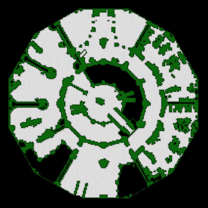
(a)

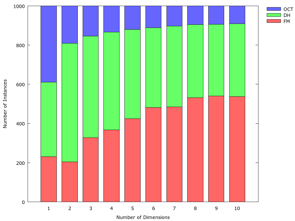
(b)

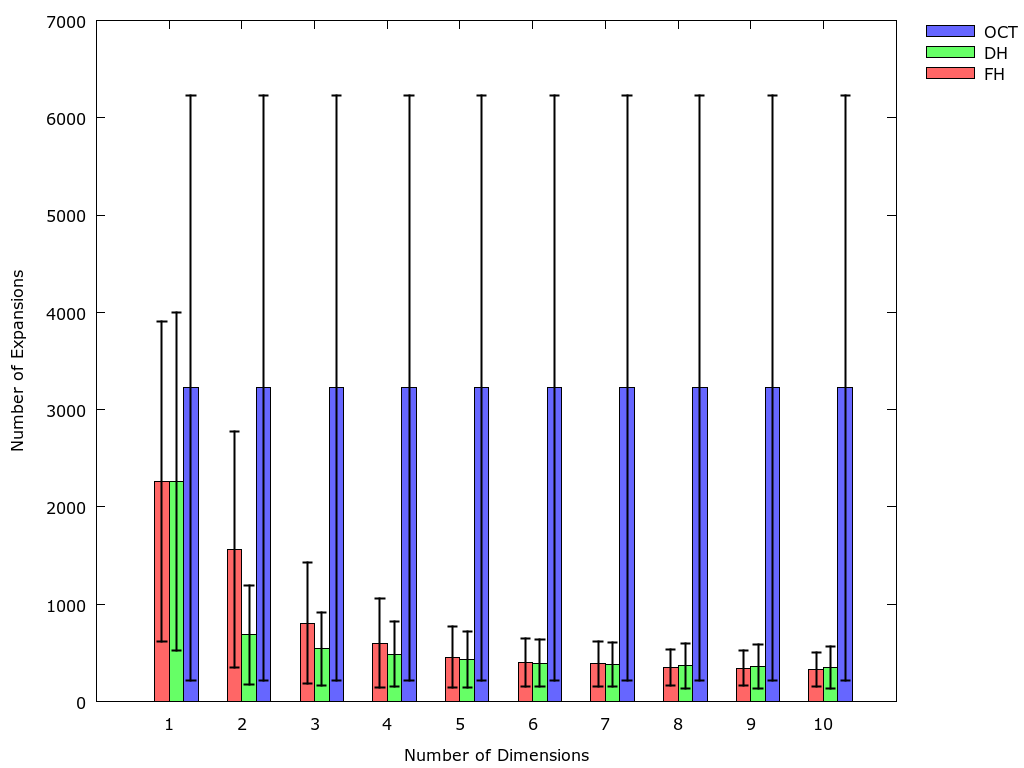
(c)

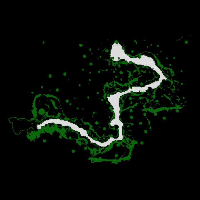
(d)

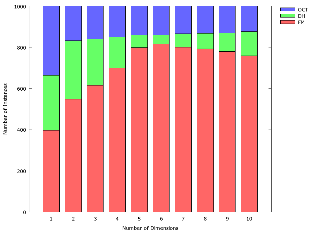
(e)

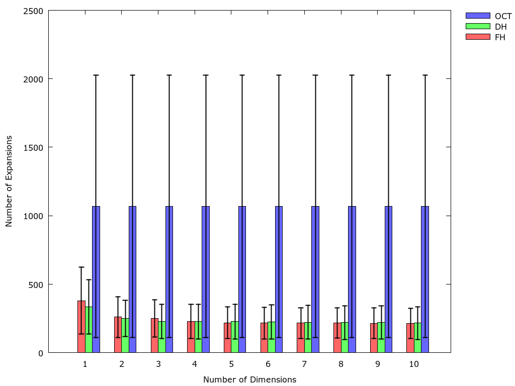
(f)

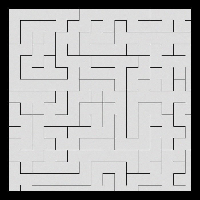
(g)

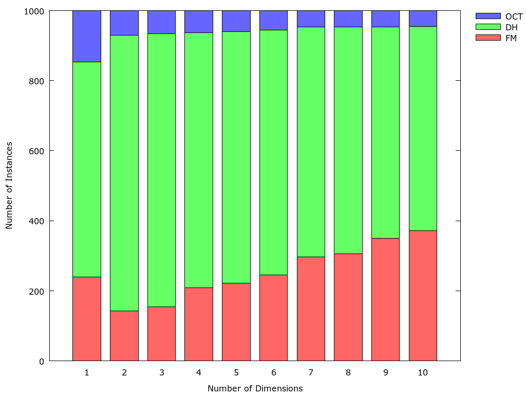
(h)

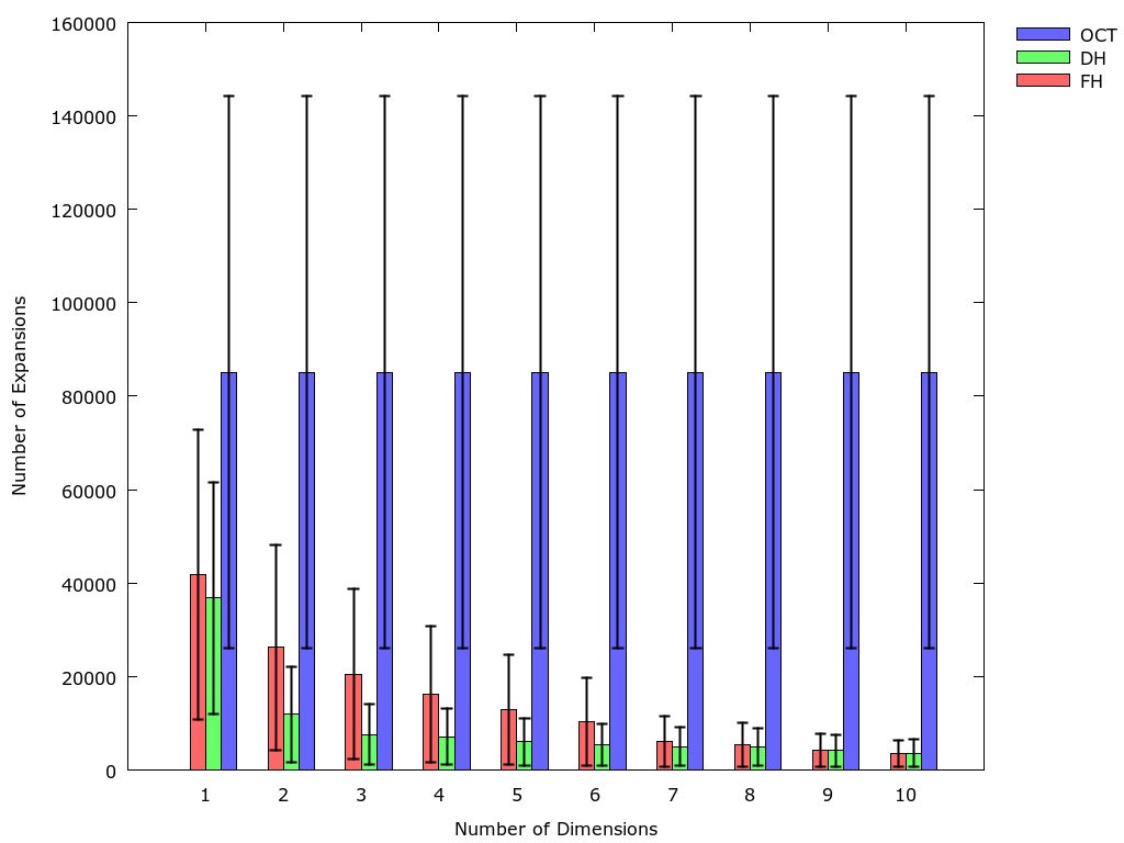
(i)

Figure 4: Shows empirical results on $3$ maps from Bioware’s Dragon Age: Origins. (a) is map ‘lak503d’ containing $17,953$ nodes and $33,781$ edges; (d) is map ‘brc300d’ containing $5,214$ nodes and $9,687$ edges; and (g) is map ‘maze512-32-0’ containing $253,840$ nodes and $499,377$ edges. In (b), the x-axis shows the number of dimensions for the FastMap heuristic (or the number of pivots for the Differential heuristic). The y-axis shows the number of instances (out of $1,000$) on which each technique expanded the least number of nodes. Each instance has randomly chosen start and goal nodes. (c) shows the median number of expanded nodes across all instances. Vertical error bars indicate the MADs. The figures in the second and third rows follow the same order. In the legends, “FM” denotes the FastMap heuristic, “DH” denotes the Differential heuristic and “OCT” denotes the Octile heuristic.

Conclusions

In this paper, we presented a near-linear time preprocessing algorithm, called FastMap, for producing a Euclidean embedding of a general edge-weighted undirected graph. At runtime, the Euclidean distances were used as heuristic by A* for shortest path computations. We proved that the FastMap heuristic is admissible and consistent, thereby generating shortest paths. FastMap produces the Euclidean embedding in near-linear time, which is significantly faster than competing approaches for producing Euclidean embeddings with optimality guarantees that run in cubic time. We also showed that it is competitive with other state-of-the-art heuristics derived in near-linear preprocessing time. However, FastMap has the combined benefits of requiring only near-linear preprocessing time and producing explicit Euclidean embeddings that try to recover the underlying manifolds of the given graphs.

References

- Alpaydin [2010] Ethem Alpaydin. Introduction to Machine Learning. The MIT Press, 2nd edition, 2010.
- Björnsson and Halldórsson [2006] Yngv Björnsson and Kári Halldórsson. Improved heuristics for optimal path-finding on game maps. In Proceedings of the 6th AAAI Conference on Artificial Intelligence and Interactive Digital Entertainment, 2006.
- Botea and Harabor [2013] Adi Botea and Daniel Harabor. Path planning with compressed all-pairs shortest paths data. In Proceedings of the 23rd International Conference on Automated Planning and Scheduling, 2013.
- Botea et al. [2004] Adi Botea, Martin Müller, and Jonathan Schaeffer. Near optimal hierarchical path-finding. Journal of Game Development, 1, 2004.
- Cazenave [2006] Tristan Cazenave. Optimizations of data structures, heuristics and algorithms for path-finding on maps. In Proceedings of the IEEE Symposium on Computational Intelligence and Games, 2006.
- Dechter [2003] Rina Dechter. Constraint processing. The Morgan Kaufmann Series in Artificial Intelligence. Elsevier, 2003.
- Dijkstra [1959] Edsger W. Dijkstra. A note on two problems in connexion with graphs. Numerische Mathematik, 1(1), 1959.
- Faloutsos and Lin [1995] Christos Faloutsos and King-Ip Lin. Fastmap: A fast algorithm for indexing, data-mining and visualization of traditional and multimedia datasets. In Proceedings of the ACM SIGMOD International Conference on Management of Data, 1995.
- Fredman and Tarjan [1984] Michael Fredman and Robert Tarjan. Fibonacci heaps and their uses in improved network optimization algorithms. Proceedings of the 25th Annual Symposium on Foundations of Computer Science, 1984.
- Geisberger et al. [2008] Robert Geisberger, Peter Sanders, Dominik Schultes, and Daniel Delling. Contraction hierarchies: Faster and simpler hierarchical routing in road networks. In Proceedings of the 7th International Conference on Experimental Algorithms, 2008.
- Goldenberg et al. [2010] Meir Goldenberg, Ariel Felner, Nathan Sturtevant, and Jonathan Schaeffer. Portal-based true-distance heuristics for path finding. In Proceedings of the 3rd Annual Symposium on Combinatorial Search, 2010.
- Goldenberg et al. [2011] Meir Goldenberg, Nathan Sturtevant, Ariel Felner, and Jonathan Schaeffer. The compressed differential heuristic. In Proceedings of the 25th AAAI Conference on Artificial Intelligence, 2011.
- Hart et al. [1968] Peter E. Hart, Nils J. Nilsson, and Bertram Raphael. A formal basis for the heuristic determination of minimum cost paths. IEEE Transactions on Systems, Science, and Cybernetics, SSC-4(2), 1968.
- Holte et al. [1994] Robert Holte, Chris Drummond, M. B. Perez, Robert Zimmer, and Alan Macdonald. Searching with abstractions: A unifying framework and new high-performance algorithm. In Proceedings of the 10th Canadian Conference on Artificial Intelligence, 1994.
- LaValle [2006] Steven LaValle. Planning Algorithms. Cambridge University Press, New York, NY, USA, 2006.
- Leighton et al. [2008] Michael Leighton, Wheeler Ruml, and Robert Holte. Faster optimal and suboptimal hierarchical search. In Proceedings of the 1st International Symposium on Combinatorial Search, 2008.
- Pochter et al. [2010] Nir Pochter, Aviv Zohar, Jeffery Rosenschein, and Ariel Felner. Search space reduction using swamp hierarchies. In Proceedings of the 24th AAAI Conference on Artificial Intelligence, 2010.
- Rayner et al. [2011] Chris Rayner, Michael Bowling, and Nathan Sturtevant. Euclidean heuristic optimization. In Proceedings of the 25th AAAI Conference on Artificial Intelligence, 2011.
- Russell and Norvig [2009] Stuart J. Russell and Peter Norvig. Artificial Intelligence: A Modern Approach. Prentice Hall, 2009.
- Storandt [2013] Sabine Storandt. Contraction hierarchies on grid graphs. In Proceedings of KI: the 36th Annual German Conference on Artificial Intelligence, 2013.
- Strasser et al. [2015] Ben Strasser, Adi Botea, and Daniel Harabor. Compressing optimal paths with run length encoding. Journal of Artificial Intelligence Research, 54:593–629, 2015.
- Sturtevant and Buro [2005] Nathan Sturtevant and Michael Buro. Partial pathfinding using map abstraction and refinement. In Proceedings of the 20th AAAI Conference on Artificial Intelligence, 2005.
- Sturtevant et al. [2009] Nathan Sturtevant, Ariel Felner, Max Barrer, Jonathan Schaeffer, and Neil Burch. Memory-based heuristics for explicit state spaces. In Proceedings of the 21st International Joint Conference on Artificial Intelligence, 2009.
- Sturtevant [2012] Nathan Sturtevant. Benchmarks for grid-based pathfinding. Transactions on Computational Intelligence and AI in Games, 4(2), 2012.
- Torgerson [1952] Warren S. Torgerson. Multidimensional scaling: I. theory and method. Psychometrika, 17(4), 1952.
- Uras and Koenig [2014] Tansel Uras and Sven Koenig. Identifying hierarchies for fast optimal search. In Proceedings of the 28th AAAI Conference on Artificial Intelligence, 2014.
- Uras and Koenig [2015] Tansel Uras and Sven Koenig. Subgoal graphs for fast optimal pathfinding. In Steve Rabin, editor, Game AI Pro 2: Collected Wisdom of Game AI Professionals, chapter 15. A K Peters/CRC Press, 2015.
- Vandenberghe and Boyd [1996] Lieven Vandenberghe and Stephen Boyd. Semidefinite programming. SIAM Review, 38, 1996.