Scattering of point particles by black holes: gravitational radiation

Abstract

Gravitational waves can teach us not only about sources and the environment where they were generated, but also about the gravitational interaction itself. Here we study the features of gravitational radiation produced during the scattering of a point-like mass by a black hole. Our results are exact (to numerical error) at any order in a velocity expansion, and are compared against various approximations. At large impact parameter and relatively small velocities our results agree to within percent level with various post-Newtonian and weak-field results. Further, we find good agreement with scaling predictions in the weak-field/high-energy regime. Lastly, we achieve striking agreement with zero-frequency estimates.

I Introduction

The momentous direct detection of gravitational waves (GWs) by the LIGO collaboration  Abbott et al. (2016a, b, 2017) provided the strongest evidence to date that black holes (BHs) exist, merge, and that the GWs produced in the strong-field regime are well described by Einstein’s theory. As more sensitive detectors come online, precise tests of strong-field gravity will become possible Gair et al. (2013); Yunes and Siemens (2013); Berti et al. (2015). Deviations from the Kerr geometry will be imprinted, for example, in the way that BHs ‘vibrate’ Berti et al. (2006, 2016). Fundamental issues – such as the existence of horizons in our universe cloaking spacetime singularities – can finally be addressed by either looking at smoking-gun signs of surfaces (such as ‘echoes’) Cardoso et al. (2016a, b) or the way that the inspiral proceeds Maselli et al. (2017); Sennett et al. (2017). Recent research into the GWs produced by compact binaries has been dominated by the study of bound motion, which is becoming quite well understood. Thus, we feel it is an appropriate time to refocus attention on the unbound binary problem.

GWs are also the perfect tool to understand gravity at its extreme. High-energy collisions of BHs produce the largest luminosities in the universe, which are thought to saturate the Dyson-Gibbons-Thorne bound ($c^{5}/G$) on this quantity Cardoso (2013). High-energy collisions of particles are expected to be universal. At large enough center-of-mass energy, the end state is always a BH and the details of the initial state are forever hidden behind its horizon Choptuik and Pretorius (2010); Sperhake et al. (2013); Cardoso et al. (2015). Recently, it was argued that the scattering of two particles at large enough energies and small deflection angles has some interesting properties, that the spectrum of graviton emission takes a simple and elegant limiting form, which can be used to learn about the S-matrix of quantum gravity Gruzinov and Veneziano (2016); Ciafaloni et al. (2015).

With the above as motivation, we start here the investigation of scattering of particles by BHs. In this work we focus primarily on the low/medium-energy regime where particle speeds (at infinite separation) do not exceed $0.25c$. We also briefly explore high-energy events with with speeds reaching $0.98c$. In the future we plan to use the code that we have developed here to more-thoroughly explore the high energy regime. There have been a number of approximate, analytic works done over the years. Of particular interest are works by Peters Peters (1970), Smarr Smarr (1977), Kovacs and Thorne Kovacs and Thorne (1978), Turner Turner (1977), and Blanchet and Schäfer Blanchet and Schaefer (1989), all of which we compare to here.

The remaining of this paper is organized as follows. Sec. II establishes notation regarding the physical system we are studying and presents the numerical method we use to solve the first-order Einstein equations. Sec. III presents known analytic predictions and our results found by comparing with those expressions. Sec. IV provides brief concluding remarks. Throughout this paper, unless otherwise mentioned, we use Schwarzschild coordinates $t,r,\theta,\phi$, and a subscript $p$ indicates a field evaluated at the particle’s location. We work in coordinates where $G=c=1$, although we do explicitly include factors of $G$ and $c$ in some expressions when it adds clarity.

II Setup and numerical procedure

II.1 Scattering geodesics on Schwarzschild

We consider point particle (mass $\mu$) motion on a Schwarzschild background (mass $M$). Take the worldline to be parametrized by proper time $\tau$, i.e. $x_{p}^{\mu}(\tau)$, with associated four-velocity is $u^{\mu}=dx_{p}^{\mu}/d\tau$. We confine the particle to $\theta_{p}=\pi/2$ without loss of generality and hence write $x^{\mu}_{p}(\tau)=\left[t_{p}(\tau),r_{p}(\tau),\pi/2,\phi_{p}(\tau)\right]$. Generic geodesics are best parametrized by the constants of motion, $\mathcal{E}$ and $\mathcal{L}$, respectively, the specific energy and angular momentum. They relate to the four-velocity via

$$u^{t}=\frac{\mathcal{E}}{f_{p}}\,,\quad\quad u^{\varphi}=\frac{{\cal{L}}}{r_{p}^{2}}\,,\quad\quad\left(u^{r}\right)^{2}=\mathcal{E}^{2}-U^{2}_{p}\,,$$ (1)

where the effective potential is

$$U^{2}(r,\mathcal{L}^{2})\equiv f\left(1+\frac{\mathcal{L}^{2}}{r^{2}}\right),$$ (2)

and $f\equiv 1-2M/r$.

For scattering geodesics, it is convenient to replace $\mathcal{L}$ with either the periapsis $r_{\rm min}$ or the impact parameter $b$. The former is related to $\mathcal{E}$ and $\mathcal{L}$ via $U^{2}(r_{\rm min},\mathcal{L}^{2})=\mathcal{E}^{2}$, while the latter is defined as $b\equiv\mathcal{L}/\sqrt{\mathcal{E}^{2}-1}.$ Note that $b\to\infty$ when $\mathcal{E}=1$, making $r_{\rm min}$ the preferable choice in the case of parabolic motion.

II.2 The frequency domain, RWZ formalism for unbound motion

We developed a new perturbation theory code to obtain the numerical results presented in this work. While the details of that code and its method will be discussed in an accompanying paper Hopper (2017), here we provide a brief summary. We use the Regge-Wheeler-Zerilli (RWZ) Regge and Wheeler (1957); Zerilli (1970) formalism wherein the field equations of any radiative $\ell m$ mode reduce to a single 1+1 wave equation,

$$\left[-\frac{\partial^{2}}{\partial t^{2}}+\frac{\partial^{2}}{\partial r_{*}^{2}}-V_{\ell}(r)\right]\Psi_{\ell m}(t,r)=S_{\ell m}(t,r).$$ (3)

Here $r_{*}$ is the usual tortoise coordinate, $r_{*}=r+2M\log(r/2M-1)$. The ‘master function’ $\Psi_{\ell m}$, its source $S_{\ell m}$ and the potential $V_{\ell}$ are all $\ell+m$ parity-dependent. We choose to work in the frequency domain (FD), and thus assume that the field and its source, can be represented by integrals over Fourier harmonics,

$$\begin{split}\Psi_{\ell m}(t,r)&=\frac{1}{2\pi}\int_{-\infty}^{\infty}X_{\ell m\omega}(r)\,e^{-i\omega t}d\omega\,,\\ S_{\ell m}(t,r)&=\frac{1}{2\pi}\int_{-\infty}^{\infty}Z_{\ell m\omega}(r)\,e^{-i\omega t}d\omega\,.\end{split}$$ (4)

In the FD the master equation (3) takes on the following form

$$\left[\frac{d^{2}}{dr_{*}^{2}}+\omega^{2}-V_{\ell}(r)\right]X_{\ell m\omega}(r)=Z_{\ell m\omega}(r).$$ (5)

At infinity and the horizon we take as boundary conditions retarded, unit-amplitude, homogeneous traveling waves,

$$\hat{X}^{\pm}_{\ell m\omega}(r_{*}\to\pm\infty)=e^{\pm i\omega r_{*}}.$$ (6)

The solution to Eq. (5) follows from the method of variation of parameters,

$$X_{\ell m\omega}(r)=c^{+}_{\ell m\omega}(r)\,\hat{X}^{+}_{\ell m\omega}(r)+c^{-}_{\ell m\omega}(r)\,\hat{X}^{-}_{\ell m\omega}(r),$$ (7)

where

$$\begin{split}c^{+}_{\ell m\omega}(r)&=\frac{1}{W_{\ell m\omega}}\,\int_{2M}^{r}\frac{dr^{\prime}}{f(r^{\prime})}\ \hat{X}^{-}_{\ell m\omega}(r^{\prime})\,Z_{\ell m\omega}(r^{\prime})\,,\\ c^{-}_{\ell m\omega}(r)&=\frac{1}{W_{\ell m\omega}}\,\int_{r}^{\infty}\frac{dr^{\prime}}{f(r^{\prime})}\ \hat{X}^{+}_{\ell m\omega}(r^{\prime})\,Z_{\ell m\omega}(r^{\prime})\,,\end{split}$$ (8)

and $W_{\ell m\omega}$ is the (constant-in-$r_{*}$) Wronskian. Extending the integrals in Eq. (8) over all space provides the normalization coefficients,

$$C_{\ell m\omega}^{\pm}=\frac{1}{W_{\ell m\omega}}\int_{2M}^{\infty}\frac{dr}{f}\ \hat{X}^{\mp}_{\ell m\omega}(r)Z_{\ell m\omega}(r).$$ (9)

These coefficients are all that one needs to compute radiated energy and waveforms, which we find in this work. The details of solving Eq. (9) (which makes up the brunt of our numerical calculation) are involved. In particular, the FD source term $Z_{\ell m\omega}$ depends on the particular choice of master function, a choice which affects the convergence of the integral in Eq. (9). As mentioned, this will be covered in detail in an accompanying work.

Assuming we have solved Eq. (9) for a range of harmonics, we compute the waveform at retarded time $u=t-r_{*}$ and $r_{*}\to\infty$ via

$$\Psi_{\ell m}(u,r_{*}\to\infty) =\frac{1}{2\pi}\int_{-\infty}^{\infty}C^{+}_{\ell m\omega}\,e^{-i\omega u}d\omega.$$ (10)

This follows because, as $r_{*}\to\infty$ the FD particular solutions go to $X^{+}_{\ell m\omega}(r_{*}\to\infty)=C^{+}_{\ell m\omega}e^{i\omega r_{*}}$. One can sum these over $\ell$ and $m$ to form the transverse-traceless metric perturbation, as shown in Ref. Martel and Poisson (2005).

Our code also provides flux and energy spectrum results. When using the Zerilli-Moncrief Moncrief (1974) (for $\ell+m$ even) and Cunningham-Price-Moncrief Cunningham et al. (1978) ($\ell+m$ odd) variables, the energy flux at infinity is

$$\dot{E}^{+}_{\ell m}(u,r_{*}\to\infty)=\frac{1}{64\pi}\frac{(\ell+2)!}{(\ell-2)!}\left|\dot{\Psi}^{+}_{\ell m}(u,r_{*}\to\infty)\right|^{2}.$$ (11)

Then, the total energy radiated for a given $\ell m$ mode to infinity is

$$E^{+}_{\ell m}=\frac{1}{128\pi^{2}}\frac{(\ell+2)!}{(\ell-2)!}\int\omega^{2}\left|C^{\pm}_{\ell m\omega}\right|^{2}d\omega\,.$$ (12)

In practice, we discretize the integrals (10) and (12) (the smallest frequencies our machine-precision code can reach are $\sim 10^{-6}/M$). Then, we add positive and negative harmonics until the total radiated energy converges to a relative error of at most 0.1% (in practice we usually achieve a much greater level of accuracy). As shown in later sections, our greatest limitation is the small (in magnitude) frequencies, in particular, for systems with very large $r_{\rm min}$.

For most of the results we compare to in this paper, we do not require modes of $\ell>6$. However, for the high-energy results given below in Sec. III.1, we do need higher $\ell$ modes. Given the modest accuracy requirements of this work, we are able to truncate out $\ell$-sum at 8 at which point we can clearly see the exponential convergence and fit out higher-order contributions to the sum. This saves computational time and gives results accurate to better than 1%.

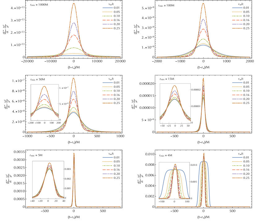
Figure 1: Energy flux for a range of scattering trajectories. Note the extended period of near-constant flux when $v_{\infty}=0.01c$ and $r_{\rm min}=4M$.

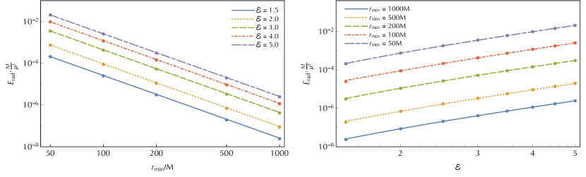
Figure 2: Total radiation as a function of $r_{\rm min}$ (left) and $\mathcal{E}$ (right) for our high-energy runs. The lines connecting the dots are fits to our data as predicted by Eq. (14).

III Gravitational waves from point-particle scattering

In this paper we are largely focused on the low-energy regime, and as such the majority of our numerical runs (nearly 150 of them) explore speeds of $0.1c\leq v_{\infty}\leq 0.25c$ and periapses with $4M\leq r_{\rm min}\leq 1000M$. We also performed 40 runs with large energies $0.75c\lesssim v_{\infty}\lesssim 0.98c$ for periapses from $r_{\rm min}=50M$ to $r_{\rm min}=1000M$. Our numerical results are summarized in Figs. 1-7. Before examining the degree of numerical agreement between our results and various analytic predictions, we note some qualitative features evident in our figures.

Emission of GWs is most effective for high-velocity, abruptly changing motion. Thus, high velocities and small periapses give rise to larger luminosities. This is shown in Fig. 1, where periapsis corresponds to $t-r_{*}=0$. Notice that the timescale over which emission occurs is not very sensitive on the initial velocity, but depends mostly on the gravitational potential at periapsis. The luminosity changes by several orders of magnitude from $r_{\rm min}=1000M$ to $r_{\rm min}=4M$. Close to $r=4M$ new features set in. For example, the timescale for energy emission increases for small velocities. This feature is related solely to geodesic motion: For small velocities, $r=4M$ is the capture threshold for incoming particles. Thus, the (point) particle can perform a large number of orbits before being scattered. Essentially then, the flux is dictated by the circular orbit of similar radius. This property was also observed for plunges with large angular momentum Berti et al. (2010), and has a visible impact on the waveform, as we show in Fig. 6, and the spectrum in Fig. 7 (see bottom panels). These features are discussed in further detail below in Sec. III.4.

We now turn attention to the numerous analytical predictions that have been made for scattering events over the years. In the following subsections we compare our numerical results with weak-field, post-Newtonian (PN) and zero-frequency limit (ZFL) predictions.

III.1 Weak-field predictions

Peters Peters (1970) made a number of weak-field predictions, two of which concern us here. His results are valid when deflection angles are small and velocities are constant.

First, in the limit of small velocities he obtains

$$\frac{E_{\rm rad}}{M}=\frac{37\pi}{15}\frac{G^{3}}{c^{5}}\left(\frac{\mu}{M}\right)^{2}\frac{v}{(r_{\rm min}/M)^{3}}.$$ (13)

From a numerical comparison standpoint, the low-and-constant velocity regime is challenging to explore since the particle is always sped up as it approaches the BH. Our most-appropriate run is $r_{\rm min}=1000M$, $v_{\infty}=0.25c$. While this trajectory is not particularly slow, it is nearly constant-speed ($v_{\rm max}=0.253c$) with small deflection angle, $1.9^{\circ}$. In this case, our numerical value of $E_{\rm rad}=2.14\times 10^{-9}\mu^{2}/M$ is within $10\%$ of Peters’ prediction in Eq. (13). Meanwhile an event with the same $r_{\rm min}=1000M$, but $v_{\infty}=0.01c$ deflects by an angle $131^{\circ}$ and has a maximum speed of $v_{\rm max}=0.045c$. Unsurprisingly, in this case, we disagree with Peters’ prediction by an order of magnitude.

Peters also explores the high-energy limit, where he finds the order-of-magnitude estimate

$$\frac{E_{\rm rad}}{M}\sim\frac{G^{3}}{c^{4}}\left(\frac{\mu}{M}\right)^{2}\frac{{\cal E}^{3}}{(r_{\rm min}/M)^{3}}\,.$$ (14)

Constant velocities and high-energy are a natural fit, and therefore we are able to explore the ultrarelativistic regime more thoroughly, with results shown in Fig. 2. All the high-energy runs we consider have nearly constant speeds (within 1%). Deflection angles range between $6.6^{\circ}$ ($r_{\rm min}=50M$, ${\cal E}=1.5$) and $0.2^{\circ}$ ($r_{\rm min}=1000M$, ${\cal E}=5$). We first check the $(r_{\rm min}/M)^{-3}$ scaling of radiation, as shown in Eq. (14). In the left panel of Fig. 2 we fit $(r_{\rm min}/M)^{-3}$ lines to the data for several energies and see the expected behavior. Our results are also consistent with an ${\cal E}^{3}$ dependence of the total radiated energy, at large and constant $r_{\rm min}$. This can be seen in the right panel of the same figure. For several values of $r_{\rm min}$ we fit a function of the form $(A\mathcal{E}^{3}+B\mathcal{E}^{2}+C\mathcal{E})\cdot(r_{\rm min}/M)^{-3}$. While there is variation in the values of the $B$ and $C$ terms, we find consistent leading-order behavior and are able to predict that the missing coefficient in Eq. (14) is $28\pm 2$.

III.2 Post-Newtonian expressions

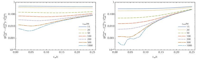
Figure 3: The relative error between our numerical values and PN predictions, Eq. (15), of the radiated energy for a range of scattering runs. For low velocities we see the expected convergence with PN order, but at higher speeds (where the approximation $v_{\infty}^{2}\sim GM/r_{\rm min}$ breaks down severely) the 1PN term actually worsens agreement. The unevenness of the $r_{\rm min}=1000M$ line in the right panel likely indicates that we have reached the floor of our numerical accuracy.

In a PN expansion, the radiated energy from a scattering event can be written in form

$$\frac{E_{\rm rad}}{M}=\frac{2}{15c^{5}}\frac{G^{7}}{(\mathcal{L}/M)^{7}}\frac{\mu^{2}}{M^{2}}\left(\mathcal{F}_{0}+\frac{1}{c^{2}}\mathcal{F}_{1}+\cdots\right),$$ (15)

where

$$\begin{split}&\mathcal{F}_{0}=\Big{(}96+292e_{r}^{2}+37e_{r}^{4}\Big{)}\arccos(-1/e_{r})\\ &\hskip 21.52771pt+\frac{\sqrt{e_{r}^{2}-1}}{3}(602+673e_{r}^{2}),\end{split}$$ (16)

$$\mathcal{F}_{1}=\frac{G^{2}}{(\mathcal{L}/M)^{2}}\bigg{[}\frac{1}{56}\arccos(-1/e_{r})$$

$$\hskip 17.22217pt\times\Big{(}52624+117288e_{r}^{2}+94542e_{r}^{4}+17933e_{r}^{6}\Big{)}$$ (17)

$$+\frac{\sqrt{e_{r}^{2}-1}}{840}\Big{(}1516596+1447788e_{r}^{2}+1271421e_{r}^{4}\Big{)}\bigg{]},$$

and

$$\begin{split}e_{r}^{2}=&1+2(\mathcal{E}-1)\frac{\mathcal{L}^{2}}{G^{2}M^{2}}\\ &+\frac{\mathcal{E}-1}{c^{2}}\left[-12-15(\mathcal{E}-1)\frac{\mathcal{L}^{2}}{G^{2}M^{2}}\right]\,.\end{split}$$ (18)

As we are only interested in the point-particle limit, we have dropped all higher-order terms in $\mu/M$ above. The lowest order term ($\mathcal{F}_{0}$) is the scattering equivalent of the Peters-Mathews result Peters and Mathews (1963), derived correctly first by Turner Turner (1977) (see also previous work Hansen (1972)). Subsequently, Blanchet and and Schäfer Blanchet and Schaefer (1989) found the next-to-leading order term $\mathcal{F}_{1}$. They used the quasi-Keplerian formalism Damour and Deruelle (1985) wherein the Newtonian eccentricity ‘splits’ into three eccentricities after leading order. The above expressions use the ‘$r$-eccentricity’.

The results of our comparison with these PN predictions are summarized in Fig. 3, with the 0PN residual on the left and 1PN residual on the right. We find expected order-of-magnitude agreement for low velocities, but around $v_{\infty}=0.1c$ the agreement starts to fail. Once we reach $v_{\infty}=0.25c$, the 1PN term actually worsens the agreement for all $r_{\rm min}$. At first glance this is a very puzzling result. However, we believe these features are correct, as a comparison with the bound, eccentric case makes clear.

The PN expansion of the orbit-averaged eccentric-motion flux can be written in the form that is highly analogous to Eq. (15) (see, e.g. Blanchet (2014)),

$$\left\langle\frac{dE}{dt}\right\rangle=\frac{32c^{5}}{5G}\nu^{2}y^{5}\Big{(}\mathcal{I}_{0}+y\mathcal{I}_{1}+y^{3/2}\mathcal{I}_{3/2}+\cdots\Big{)},$$ (19)

where the ${\cal I}_{i}$ terms are ‘enhancement factors’ akin to the ${\cal F}_{i}$ terms above. The PN parameter $y\equiv\left(GM\Omega_{\phi}/c^{3}\right)^{2/3}$ is a natural gauge invariant in which to expand, defined using the observable $\Omega_{\phi}$, the average advance in the particle’s azimuthal position. It is of the same order as $v^{2}/c^{2}$ and $GM/(c^{2}r)$. Here $v$ and $r$ are the characteristic speed and separation of the eccentric binary.

A scattering system does not exhibit such a clear PN parameter [hence, the counting of PN orders with $c^{-2}$ in Eq. (15)]. The natural length scale of the problem is $r_{\rm min}$, but since the system is unbound, we do not find that $GM/r_{\rm min}\sim v_{\infty}^{2}$ in general. As can be seen in Fig. 3, this leads to less-than-uniform convergence in PN order when we vary the speed of our scattering particle. This can be contrasted with similar PN comparisons made for eccentric motion, where PN-order convergence exists even for high eccentricities Forseth et al. (2016). (We note that Turner and Will Turner and Will (1978) attempted to address this problem by including one order higher in the $v^{2}/c^{2}$ expansion than in the $GM/(c^{2}r)$ expansion. However, we find that their calculation neglects $GM/(c^{2}r)$ terms that are important and our agreement with their predictions is poor. Hence, we do not compare with the Turner and Will result here.)

We note in passing that for bound motion the PN expansion of the energy flux is known through 3PN Arun et al. (2008), and to much higher order in the small mass-ratio limit Forseth et al. (2016). Meanwhile, as far as we know, the scattering expression has remained at 1PN for almost thirty years. In principle, all the tools are available for an enterprising PN expert to extend the Blanchet and Schäfer Blanchet and Schaefer (1989) expression to 1.5PN and beyond.

Lastly, in addition to these PN results, Kovacs and Thorne Kovacs and Thorne (1978) provide a few more properties of the radiation emitted. For example, they show (citing Ruffini and Wheeler Ruffini and Wheeler (1971)) that the energy spectrum for low-energy scatterings behaves as

$$\frac{dE}{d\omega}=\frac{32}{5}\left(\frac{\mu M}{b}\right)^{2}\left(\frac{\omega b}{v_{\infty}}\right)^{3}e^{-2\omega b/v_{\infty}}\,,$$ (20)

in the $\omega\gg v_{\infty}/b$ limit. This is a prediction of the large-$\omega$ tail of the spectra, which we plot in Fig. 7. We fit this large-$\omega$ portion of the data from our runs to a function of the form $A\omega^{3}e^{-B\omega}$. When $r_{\rm min}$ is large, we find good agreement, even for moderately large velocities $v_{\infty}$. For example, for $r_{\rm min}=1000M,\,v_{\infty}=0.25c$, the best-fit values of $A$ and $B$ each agree with those of relation (20) to within $\sim 6\%$.

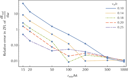
Figure 4: Error between our numerical calculation and Smarr’s analytic prediction, Eq. (21), of the energy radiated in the ZFL. Our numerical ZFL can be seen graphically by looking at the $\omega=0$ crossing of the spectra in Fig. 7. The unevenness of the lines near $r_{\rm min}\approx 100M$ is a result of zero crossings in the error.

III.3 Zero-frequency limit

The ZFL is a qualitatively interesting area of parameter space to explore. Its relevance was pointed out by Weinberg in 1964, using quantum arguments Weinberg (1964, 1965). Smarr first noticed that the ZFL can be applied successfully to classical problems of GW generation Smarr (1977); Cardoso et al. (2015). Generically, the prediction is that when two scattering bodies have non-zero speeds at infinite separation, their energy spectrum does not vanish in the ZFL. Remarkable agreement with Smarr’s calculation was found for point particles plunging into BHs Cardoso and Lemos (2002); Berti et al. (2010). Surprisingly, results of full nonlinear calculations of head-on collisions of equal mass BHs at large center-of-mass energies were in very good agreement with Smarr’s linearized estimates Sperhake et al. (2008); East and Pretorius (2013); Cardoso et al. (2015). For a scattering event, Smarr computes the ZFL of the energy spectrum to be

$$\left(\frac{dE}{d\omega}\right)_{\omega\to 0}=\frac{4}{\pi}\frac{\mu^{2}M^{2}\mathcal{E}^{2}}{b^{2}}\frac{(1+v^{2})^{2}}{v^{4}}$$ (21)

$$\hskip 43.05542pt\times\left[2-\frac{16}{3}v^{2}+\left(3v-\frac{1}{v}\right)\log\left(\frac{1+v}{1-v}\right)\right]\,.$$

His calculation assumes large impact parameters and constant velocities. We expect these assumptions to be reasonably valid when $r_{\rm min}\gg 2M$, and indeed, looking at Fig. 4, we find that for $r_{\rm min}\gtrsim 200M$ our numerical values agree with Smarr’s prediction to at least 10%. When $r_{\rm min}=1000M$ our relative errors are on the order of 1% for all velocities.

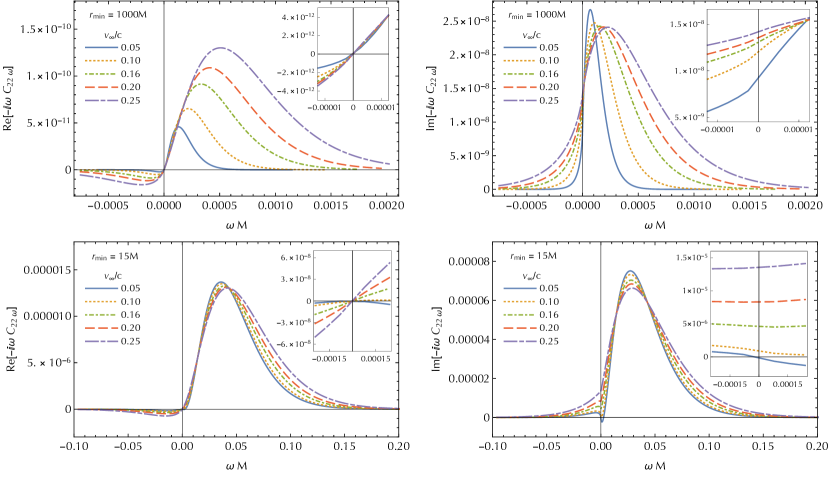
Figure 5: The $(\ell,m)=(2,2)$ contribution to the FD waveform (multiplied by $-i\omega$) for a range of scattering events with $r_{\rm min}=15M$ and $r_{\rm min}=1000M$. The spectrum is sampled everywhere (except exactly $\omega=0$) with a step size $M\Delta\omega=8\times 10^{-5}$ (for $r_{\rm min}=15M$) and $M\Delta\omega=2.5\times 10^{-6}$ (for $r_{\rm min}=1000M$). The modes are combined to form the TD waveform shown in Fig. 6, using Eq. (10). The jump in that TD waveform between $u=-\infty$ and $u=\infty$ is predicted by the ZFL here, as shown in the insets.

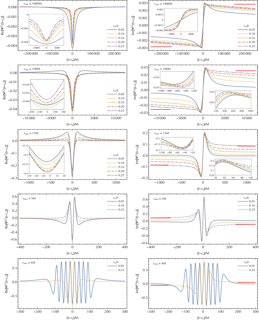
Figure 6: The $(\ell,m)=(2,2)$ contribution to the waveform for scattering events with a range of $r_{\rm min}$ and particle speeds. In the right panels a solid red line shows the prediction of the memory effect for $v_{\infty}/c=0.25$ based on the ZFL of the FD waveform shown in Fig. 5.

In addition to Smarr’s prediction of the ZFL of the energy spectrum, we can use the ZFL to evaluate the difference in $\Psi_{\ell m}$ before and after the encounter. Taking ZFL of the Fourier transform of $\partial_{u}\Psi_{\ell m}(u,r_{*})$ (and performing an integration by parts) we have

$$\begin{split}&\lim_{\omega\to 0}\int_{-\infty}^{\infty}e^{i\omega u}\partial_{u}\Psi_{\ell m}(u,r_{*})du\\ &\hskip 43.05542pt=\Psi_{\ell m}(\infty,r_{*})-\Psi_{\ell m}(-\infty,r_{*})\,.\end{split}$$ (22)

We define the jump in $\Psi_{\ell m}$ as measured at infinity to be $\left\llbracket\Psi_{\ell m}\right\rrbracket\equiv\Psi_{\ell m}(\infty,r_{*}\to\infty)-\Psi_{\ell m}(-\infty,r_{*}\to\infty).$ It can be evaluated by combining Eqs. (22) and (10),

$$\left\llbracket\Psi_{\ell m}\right\rrbracket =\lim_{\omega\to 0}\int_{-\infty}^{\infty}e^{i\omega u}\partial_{u}\left(\frac{1}{2\pi}\int_{-\infty}^{\infty}C^{+}_{\ell m\omega^{\prime}}\,e^{-i\omega^{\prime}u}d\omega^{\prime}\right)du$$

$$=-\lim_{\omega\to 0}i\omega\,C^{+}_{\ell m\omega}\,.$$ (23)

In Fig. 5 we show plots of $-i\omega C^{+}_{\ell m\omega}$, with insets showing the $\omega\approx 0$ regime. As seen in that figure, the ZFL only has an imaginary component. For trajectories that travel close to the BH, it yields precisely the expected offset in the asymptotic TD waveforms, as shown in Fig. 6. We see that there is a very good agreement for values of $r_{\rm min}\lesssim 15M$. The lack of agreement for runs with larger periapses is discussed in the next section. The offset in the TD waveform is a well-known phenomenon also called the memory effect Zel’dovich and Polnarev (1974); Christodoulou (1991). See Favata’s review Favata (2010) and references therein for a thorough discussion of the subject.

III.4 Trajectories with large and small values of $r_{\rm min}$

From a qualitative standpoint, the most interesting areas of parameter space we explore are those with very small and very large pericenters. We now consider the features of these two regimes each in turn, starting with close encounters.

The trajectory $r_{\rm min}=4M,{\cal E}=1$ is marginally bound and parabolic. A particle on this trajectory will orbit the BH an infinite number of times and radiate an infinite amount of energy (representing, of course, a breakdown in the geodesic approximation). We approach this point considering scattering events with $v_{\infty}$ as small as $0.1c,({\cal E}\approx 1.00005)$. In this case there is a clear qualitative shift in the spectrum, energy flux, and waveform relative to the other cases we consider.

Consider first the spectrum shown in the bottom left of Fig. 7. The spectrum of each $\ell$ mode is dominated by the $\ell=m$ contribution. The peak for each $\ell$ mode occurs at $\omega=m\Omega_{4M}=m/(8M)$, the $\ell=m$ harmonic of the fundamental frequency of a circular orbit at $r_{p}=4M$. The waveform for this trajectory (bottom row of Fig. 6) and the flux (bottom right of Fig. 1) show evidence of the particle zoom-whirling close to the BH. In fact, when $v_{\infty}=0.01c$, the particle remains close to the BH emitting a constant flux for nearly $200M$.

The $r_{\rm min}=4M$ runs also allow us to examine the conjectured Dyson-Gibbons-Thorne bound of a peak luminosity of (restoring physical units) $c^{5}/G$. Presumably larger luminosities are impossible to achieve since the radiation itself would then collapse to form a BH. The bottom right panel of Fig. 1 shows that our flux peaks around $dE/dt\sim 0.01\mu^{2}/M^{2}$ when $v_{\infty}=0.25c$. Thus, even when extrapolating our results to equal-mass scatters, the peak luminosity is below unity. This is an interesting result, indicating that the conjectured Dyson-Gibbons-Thorne bound holds Cardoso (2013). Trajectories with $v_{\infty}>0$ can penetrate the $r_{\rm min}=4M$ boundary, with the limit approaching $r_{\rm min}=3M$ as ${\cal E}\to\infty$ ($v_{\infty}\to c$). In a future work, we will explore how close to $r_{\rm min}=3M$ our code can reach, and, as a result, see how close to the conjectured bound these ultrarelativistic encounters bring us.

At the other extreme are runs where $r_{\rm min}$ gets very large. In this work we consider periapses as large as $1000M$. We have seen that the radiated energy trends as $r_{\rm min}^{-3}$, and so these weak field scatters radiate very weakly. Indeed, we see in Fig. 7 that their spectrum is peaked around very small frequencies. Numerically these frequencies are quite challenging for our machine-precision code. In practice our GSL GSL integrator fails below $\omega_{\rm min}=2.5\times 10^{-6}/M$. This smallest frequency provides a fundamental limit to our spectral method. It implies that any TD signal we reproduce will be periodic over a timescale of $2\pi/\omega_{\rm min}\approx 2.5\times 10^{6}M$. This effect is plainly visible in the waveforms at the top of Fig. 6 and it is the source of our disagreement with the predicted memory effect. Indeed all of our waveforms eventually repeat, but the beginning of this effect is only visible in the top two rows of waveforms, which are plotted over very long timescales. We expect that if our machine-precision code could reach arbitrarily-small frequencies, we would see the exact memory effect predicted by the ZFL.

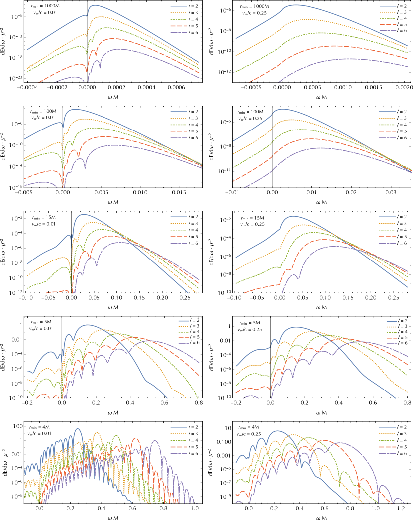
Figure 7: The radiated energy spectrum for runs with $v_{\infty}/c=0.01$ and $0.25$ and a range of $r_{\rm min}$. The top and bottom rows show spectra for the largest and smallest periapses considered. In those cases, there is a sizable effect from due to the value of $v_{\infty}$. This is most evident in the differences in axes of the plots in the left and right columns. Meanwhile, for moderate $r_{\rm min}=15M$, the trajectories with $v_{\infty}/c=0.01$ and $0.25$ yield spectra that are qualitatively quite similar.

IV Discussion

Our results are in agreement with a number of approximations made in the literature, mostly for small velocities and large impact-parameter scatters. We find strong evidence that the PN approximation is working well and converging in the regime where it should (low velocities). This study is a first step in the broader program of understanding gravitational radiation from bound and unbound motion. Left for future work is the study of high-energy scatters and plunges, and how they impact on peak luminosities (and consequences for the conjectured bound on luminosity) and other radiation properties. These questions may have some relevance for astrophysics, but they certainly have a bearing on our understanding of gravity at low- and high-energy scales.