Fully kinetic versus reduced-kinetic modelling of collisionless plasma turbulence

Abstract

We report the results of a direct comparison between different kinetic models of collisionless plasma turbulence in two spatial dimensions. The models considered include a first principles fully kinetic (FK) description, two widely used reduced models [gyrokinetic (GK) and hybrid-kinetic (HK) with fluid electrons], and a novel reduced gyrokinetic approach (KREHM). Two different ion beta ($\beta_{i}$) regimes are considered: 0.1 and 0.5. For $\beta_{i}=0.5$, good agreement between the GK and FK models is found at scales ranging from the ion to the electron gyroradius, thus providing firm evidence for a kinetic Alfvén cascade scenario. In the same range, the HK model produces shallower spectral slopes, presumably due to the lack of electron Landau damping. For $\beta_{i}=0.1$, a detailed analysis of spectral ratios reveals a slight disagreement between the GK and FK descriptions at kinetic scales, even though kinetic Alfvén fluctuations likely still play a significant role. The discrepancy can be traced back to scales above the ion gyroradius, where the FK and HK results seem to suggest the presence of fast magnetosonic and ion Bernstein modes in both plasma beta regimes, but with a more notable deviation from GK in the low-beta case. The identified practical limits and strengths of reduced-kinetic approximations, compared here against the fully kinetic model on a case-by-case basis, may provide valuable insight into the main kinetic effects at play in turbulent collisionless plasmas, such as the solar wind.

1 Introduction

Turbulence is pervasive in astrophysical and space plasma environments, posing formidable challenges for the explanation of complex phenomena such as the turbulent heating of the solar wind (Bruno & Carbone, 2013), magnetic field amplification by dynamo action (Kulsrud & Zweibel, 2008; Rincon et al., 2016; Kunz et al., 2016), and turbulent magnetic reconnection (Matthaeus & Lamkin, 1986; Lazarian & Vishniac, 1999; Loureiro et al., 2009; Matthaeus & Velli, 2011; Lazarian et al., 2015; Cerri & Califano, 2017). The average mean free path of the ionized particles in the majority of these naturally turbulent systems typically greatly exceeds the characteristic scales of turbulence, rendering the dynamics over a broad range of scales essentially collisionless. Driven by increasingly accurate in-situ observations, a considerable amount of current research is focused on understanding collisionless plasma turbulence at kinetic scales of the solar wind (Marsch, 2006; Bruno & Carbone, 2013), where the phenomenology of the inertial range (magnetohydrodynamic) turbulent cascade is no longer applicable due to collisionless damping of electromagnetic fluctuations, dispersive properties of the wave physics, and as a result of kinetic-scale coherent structure formation (Kiyani et al., 2015). The research effort with emphasis on kinetic-scale turbulence includes abundant observations (Leamon et al., 1998; Bale et al., 2005; Alexandrova et al., 2009; Sahraoui et al., 2009; Kiyani et al., 2009; Osman et al., 2011; He et al., 2012; Salem et al., 2012; Chen et al., 2013; Lacombe et al., 2014; Chasapis et al., 2015; Perrone et al., 2016; Narita et al., 2016), supported by analytical predictions (Galtier & Bhattacharjee, 2003; Howes et al., 2008a; Schekochihin et al., 2009; Boldyrev et al., 2013; Passot & Sulem, 2015), and computational studies (Howes et al., 2008b; Saito et al., 2008; Servidio et al., 2012; Verscharen et al., 2012; Boldyrev & Perez, 2012; Wu et al., 2013b; Karimabadi et al., 2013; TenBarge & Howes, 2013; Chang et al., 2014; Vasquez et al., 2014; Valentini et al., 2014; Told et al., 2015; Wan et al., 2015; Franci et al., 2015; Cerri et al., 2016; Parashar & Matthaeus, 2016).

Out of numerical convenience and based on physical considerations, the simulations of collisionless plasma turbulence are often performed using various types of simplifications of the first principles fully kinetic plasma description. Among the most prominent reduced-kinetic models for astrophysical and space plasma turbulence are the so-called hybrid-kinetic (HK) model with fluid electrons (Winske et al., 2003; Verscharen et al., 2012; Parashar et al., 2009; Vasquez et al., 2014; Servidio et al., 2015; Franci et al., 2015; Kunz et al., 2016) and the gyrokinetic (GK) model (Howes et al., 2008a, b; Schekochihin et al., 2009; TenBarge & Howes, 2013; Told et al., 2015; Li et al., 2016). Even though these models are frequently employed, no general consensus concerning the validity of reduced-kinetic treatments presently exists within the community, with distinct views on the subject being favoured by different authors (Howes et al., 2008a; Matthaeus et al., 2008; Schekochihin et al., 2009; Servidio et al., 2015). Fully kinetic (FK) simulations, on the other hand, are currently constrained by computational requirements that limit the prevalence of such studies, the accessible range of plasma parameters, and the ability to extract relevant information from the vast amounts of simulation data (Saito et al., 2008; Wu et al., 2013b; Karimabadi et al., 2013; Chang et al., 2014; Haynes et al., 2014; Wan et al., 2015; Parashar & Matthaeus, 2016). In order to spend computational resources wisely and focus fully kinetic simulations on cases where they are most needed, it is therefore crucial to establish a firm understanding of the practical limits of reduced-kinetic models. Furthermore, the question concerning the validity of reduced-kinetic approximations is not only important from the computational perspective, but is also of major interest for the development of analytical predictions based on a set of simplifying but well-validated assumptions, and for the interpretation of increasingly accurate in-situ satellite measurements. Last but not least, a thorough understanding of the range of parameters and scales where reduced models correctly reproduce the fully kinetic results is instrumental in identifying the essential physical processes that govern turbulence in those regimes.

In this work, we try to shed light on some of the above-mentioned issues by performing a systematic, first-of-a-kind comparison of the FK, HK, and GK modelling approaches for the particular case of collisionless, kinetic-scale plasma turbulence. Furthermore, we also compare the results against a novel reduced gyrokinetic model, corresponding to the low plasma beta limit of GK. Studies of similar type have been relatively rare so far (Birn et al., 2001; Henri et al., 2013; TenBarge et al., 2014; Muñoz et al., 2015; Told et al., 2016b; Camporeale & Burgess, 2017; Cerri et al., 2017; Pezzi et al., 2017a, b). Considering these circumstances, we choose here to investigate different plasma regimes in order to give a reasonably comprehensive view of the effects of adopting reduced-kinetic approximations for studying kinetic-scale, collisionless plasma turbulence. On the other hand, the simulation parameters that we select per force result from a compromise between the desire for maximal relevance of results in relation to solar wind turbulence and computational accessibility of the problem. To this end, we adopt a two-dimensional and widely-used setup of decaying plasma turbulence (Orszag & Tang, 1979) and carefully tailor the simulation parameters to reach—as much as possible—the plasma conditions relevant for the solar wind. The particular type of initial condition was chosen here for its simplicity and popularity, allowing for a relatively straightforward reproduction of our simulations and/or comparison of the results with previous works (Biskamp & Welter, 1989; Dahlburg & Picone, 1989; Politano et al., 1989, 1995; Parashar et al., 2009, 2015a; Loureiro et al., 2016; Li et al., 2016). On the other hand, it is still reasonable to expect that the turbulent system studied in this work shares at least some qualitative similarities with natural turbulence occurring at kinetic scales of the solar wind (Servidio et al., 2015; Li et al., 2016; Wan et al., 2016). We also note that the choice of initial conditions should not affect the small-scale properties of turbulence due to the self-consistent reprocess of the fluctuations by each model during the turbulent cascade (Cerri et al., 2017).

The paper is organized as follows. In Section 2 we provide a short summary of the kinetic models included in the comparison, followed by a description of the simulation setup in Sec. 3. The results presented in Sec. 4 are divided into several parts. In the first part, we investigate the spatial structure of the solutions by comparing the snapshots of the electric current and the statistics of magnetic field increments (Sec. 4.1). The analysis of turbulent structures in real space is followed by a comparison of the global turbulence energy budgets for each model (Sec. 4.2). Afterwards, we perform a detailed comparison of the spectral properties of the solutions (Sec. 4.3), followed by the analysis of the nonthermal ion and electron free energy fluctuations in the spatial domain (Sec. 4.4). Finally, we conclude the paper with a summary and discussion of our main results (Sec. 5).

2 Kinetic Models Included in the Comparison

For the sake of clarity, we provide below brief descriptions of the kinetic models involved in the comparison. However, we make no attempt to give a comprehensive overview of each model and we refer the reader to the references given below for further details. As is often done in literature, we adopt here the so-called collisionless approximation (Lifshitz & Pitaevskii, 1981; Klimontovich, 1997) as the basis for interpreting our results, given the fact that the solar wind is very weakly collisional (Marsch, 2006; Bruno & Carbone, 2013). By definition, the collisionless approximation neglects any discrete binary (and higher order) particle interactions. It is worth mentioning that although we do not explicitly consider the role of a weak collisionality, our numerical solutions still contain features which resemble (weakly) collisional effects in a plasma. In the particle-in-cell (PIC) method, collisional-like effects occur due to random statistical fluctuations in the electrostatic potential felt by each finite-size particle, and due to numerical effects related to the use of a spatial grid for the electromagnetic fields (Okuda & Birdsall, 1970; Hockney, 1971; Birdsall & Langdon, 2005). Eulerian based methods, on the other hand, are subject to an effective velocity space diffusion, which acts to smooth the particle distribution function at the smallest resolved velocity scales.

We start with a quick summary of the fully kinetic, electromagnetic plasma model (Klimontovich, 1967; Lifshitz & Pitaevskii, 1981; Klimontovich, 1997; Liboff, 2003). In the collisionless limit, the kinetic properties of a plasma are governed by the Vlasov equation for each particle species $s$:

$$\frac{\partial f_{s}}{\partial t}+\mathbf{v}\cdot\nabla f_{s}+q_{s}\left(\mathbf{E}+\frac{\mathbf{v}\times\mathbf{B}}{c}\right)\cdot\frac{\partial f_{s}}{\partial\mathbf{p}}=0,$$ (1)

where $f_{s}(\mathbf{r},\mathbf{p},t)$ is the single-particle distribution function, $q_{s}$ is the species charge, $\mathbf{v}$ is the velocity, $\mathbf{p}$ is the (relativistic) momentum, and $\mathbf{E}$ and $\mathbf{B}$ are the (smooth) self-consistent electromagnetic fields. The self-consistent fields are obtained from the full set of Maxwell equations,

$$\frac{\partial\mathbf{E}}{\partial t} =c\,\nabla\times\mathbf{B}-4\pi\mathbf{J}, \frac{\partial\mathbf{B}}{\partial t} =-\,c\,\nabla\times\mathbf{E},$$ (2)

$$\nabla\cdot\mathbf{E} =4\pi\rho, \nabla\cdot\mathbf{B} =0,$$ (3)

where $\mathbf{J}=\sum_{s}q_{s}\int\mathbf{v}f_{s}\,\mathrm{d}^{3}{\mathbf{p}}$ is the electric current and $\rho=\sum_{s}q_{s}\int f_{s}\,\mathrm{d}^{3}\mathbf{p}$ is the charge density. The above equations form a closed set for the fully kinetic description of a plasma in the collisionless limit.

The hybrid-kinetic Vlasov-Maxwell model (Byers et al., 1978; Harned, 1982; Winske et al., 2003) is a non-relativistic, quasi-neutral plasma model where the ions are fully kinetic and the electrons are treated as a background neutralizing fluid with some underlying assumption for their equation of state (typically an isothermal closure). The fundamental kinetic equation solved by the HK model is the Vlasov equation for the ions:

$$\frac{\partial f_{i}}{\partial t}+\mathbf{v}\cdot\nabla f_{i}+\frac{q_{i}}{m_{i}}\left(\mathbf{E}+\frac{\mathbf{v}\times\mathbf{B}}{c}\right)\cdot\frac{\partial f_{i}}{\partial\mathbf{v}}=0,$$ (4)

where $f_{i}(\mathbf{r},\mathbf{v})$ is the ion single-particle distribution function and $m_{i}$ is the ion mass. The $\mathbf{B}$ field is advanced using Faraday’s law

$$\frac{\partial\mathbf{B}}{\partial t} =-\,c\,\nabla\times\mathbf{E}.$$ (5)

Since the HK model assumes the non-relativistic limit, the displacement current is neglected in the Ampére’s law, which thus reads

$$\nabla\times\mathbf{B} =\,\frac{4\pi}{c}\,\mathbf{J}.$$ (6)

Finally, the electric field is obtained from the generalized Ohm’s law (Valentini et al., 2007):

$$\big{(}1-d_{e}^{2}\nabla^{2}\big{)}\mathbf{E}=-\frac{\mathbf{u}_{e}\times\mathbf{B}}{c}-\frac{\nabla p_{e}}{ne}+\eta\mathbf{J}\\ -\frac{m_{e}}{m_{i}}\left\{\frac{\mathbf{u}_{i}\times\mathbf{B}}{c}-\frac{1}{ne}\nabla\cdot\Big{[}m_{i}n(\mathbf{u}_{i}\mathbf{u}_{i}-\mathbf{u}_{e}\mathbf{u}_{e})+\boldsymbol{\Pi}_{i}\Big{]}\right\},$$ (7)

where $d_{e}$, $m_{e}/m_{i}$, $\eta$, $n$, $\mathbf{u}_{i}$, $\mathbf{u}_{e}=\mathbf{u}_{i}-\mathbf{J}/en$, $p_{e}$, and $\boldsymbol{\Pi}_{i}$ are the electron skin depth, electron-ion mass ratio, (numerical) resistivity, plasma density, ion fluid velocity, electron fluid velocity, electron pressure, and ion pressure tensor, respectively. The HK model is a quasi-neutral theory (Tronci & Camporeale, 2015), $n_{i}\simeq n_{e}\equiv n$, and therefore it deals only with frequencies much smaller than the electron plasma frequency, $\omega\ll\omega_{pe}$. We also note that the finite electron mass in expression (7) is in practice often set to zero, which consequently neglects electron inertia and results in a much simplified version of Ohm’s law:

$$\mathbf{E}=-\frac{\mathbf{u}_{e}\times\mathbf{B}}{c}-\frac{\nabla p_{e}}{ne}+\ \eta\mathbf{J}.$$ (8)

The gyrokinetic model (Frieman & Chen, 1982; Brizard & Hahm, 2007) orders fluctuating quantities according to a small expansion parameter $\epsilon$. In particular, the following ordering is assumed for the fluctuating quantities:

$$\delta f_{s}/F_{0,s}\sim\delta B/B_{0}\sim q_{s}\delta\phi/T_{0,s}\sim\epsilon,$$ (9)

where $F_{0,s}$ is the background particle distribution function, $\delta f_{s}$ is the perturbed part of the distribution, $\delta\phi$ is the perturbed electrostatic potential, $T_{0,s}$ is the background kinetic temperature (measured in energy units), and $B_{0}$ is the background magnetic field. A similar ordering is assumed for the characteristic macroscopic length scale $L_{0}$ and the frequencies of the fluctuating quantities $\omega$:

$$\omega/\Omega_{cs}\sim\rho_{s}/L_{0}\sim\epsilon,$$ (10)

where $\Omega_{cs}$ is the species cyclotron frequency and $\rho_{s}$ is the species Larmor radius. For the problems of interest, such as kinetic-scale turbulence in the solar wind (Howes et al., 2006, 2008a; Schekochihin et al., 2009), the macroscopic length scale can be typically associated with a characteristic wavelength of the fluctuations measured along the magnetic field. Time scales comparable to the cyclotron period are cancelled out by performing an averaging operation over the particle Larmor motion. The phase space is then conveniently described in terms of the coordinates $(\mathbf{R}_{s},\mu_{s},v_{\parallel})$, where $\mathbf{R}_{s}=\mathbf{r}+(\mathbf{v}\times\mathbf{b}_{0})/\Omega_{cs}$ is the particle gyrocenter position, $\mu_{s}=m_{s}v_{\perp}^{2}/2B_{0}$ is the magnetic moment, and $v_{\parallel}=\mathbf{v}\cdot\mathbf{b}_{0}$ the velocity along the mean field, where $\mathbf{b}_{0}=\mathbf{B}_{0}/B_{0}$. Instead of evolving the perturbed distribution $\delta f_{s}$, the gyrokinetic equations are typically written in terms of the ring distribution:

$$h_{s}(\mathbf{R}_{s},\mu_{s},v_{\parallel},t)=\delta f_{s}(\mathbf{r},\mathbf{v},t)+\frac{q_{s}{\delta\phi(\mathbf{r},t)}}{T_{0,s}}F_{0,s}(v).$$ (11)

The distribution $h_{s}$ is independent of the gyrophase angle at fixed $\mathbf{R}_{s}$. The electromagnetic fields are obtained self-consistently from the ring distribution under the assumption (9) and (10). For the electrostatic potential, the assumptions result in a quasineutrality condition, which is used to determine $\delta\phi$. The magnetic field, on the other hand, is obtained from a GK version of Ampere’s law.

Finally, we summarize the main features of the so-called Kinetic Reduced Electron Heating Model (KREHM) (Zocco & Schekochihin, 2011). KREHM is a fluid-kinetic model, obtained as a rigorous limit of gyrokinetics for low-beta magnetized plasmas. In particular, the low beta assumption takes the following form:

$$\sqrt{\beta_{e}}\sim\sqrt{m_{e}/m_{i}}\ll 1,$$ (12)

where $\beta_{e}$ is the electron beta ratio. Due to its low beta limit, the addition of KREHM to this work clarifies the plasma beta dependence of our results. Instead of solving for the total perturbed electron distribution function $\delta f_{e}$, KREHM is written in terms of

$$g_{e}=\delta f_{e}-(\delta n/n_{0}+2v_{\parallel}\delta u_{\parallel,e}/v_{th,e}^{2})/F_{0,e},$$ (13)

where $\delta n_{e}$ is the perturbed density, $\delta u_{\parallel,e}$ the perturbed electron fluid velocity along the mean magnetic field, and $v_{th,e}=\sqrt{2T_{0,e}/m_{e}}$ is the electron thermal velocity of the background distribution $F_{0,e}$. The modified distribution $g_{e}$ has vanishing lowest two (fluid) moments, thus highlighting the kinetic physics contained in KREHM, leading to small-scale velocity structures in the perturbed distribution function. As the final set of equations for $g_{e}$ does not explicitly depend on velocities perpendicular to the magnetic field, the perpendicular dynamics may be integrated out, leaving only the parallel velocity coordinate. As such, the model is by far the least computationally demanding of the four that we employ. As shown in Zocco & Schekochihin (2011), a convenient representation of $g_{e}$ in the $v_{\parallel}$ space can be given in terms of Hermite polynomials.

3 Problem description and simulation setup

In the following section we provide details regarding the choice of initial condition and plasma parameters. Further technical details describing the numerical settings used for each type of simulation are given in Appendix A.

The initial condition used for all simulations is the so-called Orszag-Tang vortex (Orszag & Tang, 1979)—a widely-used setup for studying decaying plasma turbulence (Biskamp & Welter, 1989; Dahlburg & Picone, 1989; Politano et al., 1989, 1995; Parashar et al., 2009, 2015a; Loureiro et al., 2016; Li et al., 2016). The initial fluid velocity and magnetic field perturbation are given by

$$\mathbf{u}_{\perp} =\delta u\,\bigl{(}-\sin(2\pi y/L)\,\hat{\mathbf{e}}_{x}+\sin(2\pi x/L)\,\hat{\mathbf{e}}_{y}\bigr{)},$$ (14)

$$\mathbf{B}_{\perp} =\delta B\,\bigl{(}-\sin(2\pi y/L)\,\hat{\mathbf{e}}_{x}+\sin(4\pi x/L)\,\hat{\mathbf{e}}_{y}\bigr{)},$$ (15)

where $L$ is the size of the periodic domain ($x,y\in[0,L)$), and $\delta u$ and $\delta B$ are the initial fluid and magnetic fluctuation amplitudes, respectively. A uniform magnetic field $\mathbf{B}_{0}=B_{0}\hat{\mathbf{e}}_{z}$ is imposed in the out-of-plane ($z$) direction. In addition to magnetic field fluctuations, we initialize a self-consistent electric current in accordance with Ampere’s law:

$$J_{z}=\frac{c}{4\pi}\frac{2\pi\delta B}{L}\bigl{(}2\cos(4\pi x/L)+\cos(2\pi y/L)\bigr{)}.$$ (16)

For the FK and GK simulations, we explicitly initialize the parallel current via a locally shifted Maxwellian for the electron species. Similarly, we prescribe the perpendicular fluid velocities for the FK and HK models by locally shifting the Maxwellian velocity distributions in $v_{x}$ and $v_{y}$. For GK and KREHM, the same approach is not possible due to the gyrotropy assumption imposed on the particle perpendicular velocities. Instead, the in-plane fluid velocities for GK and KREHM are set up with a plasma density perturbation, resulting in self-consistent electrostatic field that gives rise to perpendicular fluid motions via the $\mathbf{E}\times\mathbf{B}$ drift (Numata et al., 2010; Loureiro et al., 2016). In the large-scale and strong guide field limit, the leading order term for the electric field is

$$\mathbf{E}_{\perp}\approx-\frac{1}{c}\mathbf{u}_{\perp}\times\mathbf{B}_{0}$$ (17)

and the perturbation is electrostatic. For better consistency with reduced-kinetic models used here, the $\mathbf{E}$ field for the FK model is initialized according to Eq. (17) with a corresponding (small) electron density perturbation to satisfy the Poisson equation for the electrostatic potential. Apart from minor density fluctuations that account for the electrostatic field, the initial ion and electron densities, as well as temperatures, are chosen to be uniform. Finally, it is important to mention that we perform the HK simulations with the generalized version of Ohm’s law given by Eq. (7) which includes electron inertia, and as such features a collisionless mechanism for breaking the magnetic field frozen-in flux constraint.

A list of simulation runs with the corresponding plasma parameters and box sizes is given in Table 1. The key dimensionless parameters varied between the runs are the ion beta

$$\beta_{i}=8\pi n_{0}T_{i}/B_{0}^{2}$$ (18)

and the initial turbulence fluctuation strength

$$\epsilon=\delta B/B_{0}=\delta u/v_{A},$$ (19)

where $v_{A}=B_{0}/\sqrt{4\pi n_{0}m_{i}}$ is the Alfvén speed. Throughout this article, the species thermal velocity is defined as $v_{th,s}=\sqrt{2T_{s}/m_{s}}$ and the species Larmor radius is given by $\rho_{s}=v_{th,s}/\Omega_{cs}$, where $\Omega_{cs}=eB/(m_{s}c)$ is the species cyclotron frequency. Unless otherwise stated, lengths are normalized to the ion inertial length $d_{i}=\rho_{i}/\sqrt{\beta_{i}}$, velocities to the Alfvén speed $v_{A}$, masses to the ion mass $m_{i}$, magnetic field to $B_{0}$, the electric field to $v_{A}B_{0}/c$, and density to the background value $n_{0}$. We take the (integral scale) eddy turnover time $\tau_{0}$ as the basic time unit, which we define here as

$$\tau_{0}=\frac{L}{2\pi\delta u}.$$ (20)

The eddy turnover time, being independent of kinetic quantities, is a robust measure allowing for a direct comparison of simulations obtained from different plasma models and for variable fluctuation levels and box sizes (Parashar et al., 2015a). Further simulation details pertaining to each kinetic model are provided in Appendix A.

Main plasma parameters
Run	$\beta_{i}$	$\epsilon$	$m_{i}/m_{e}$	$T_{i}/T_{e}$	$L/d_{i}$
A1	0.1	0.2	100	1	$8\pi$
A2	0.1	0.1	100	1	$8\pi$
B1	0.5	0.3	100	1	$8\pi$
B2	0.5	0.15	100	1	$8\pi$

Table 1: List of simulation runs with their corresponding plasma parameters: ion beta ($\beta_{i}$), initial turbulence fluctuation level ($\epsilon$), ion-electron mass ratio ($m_{i}/m_{e}$), ion-electron temperature ratio ($T_{i}/T_{e}$), and box size in units of the ion inertial length ($L/d_{i}$).

4 Results

Below we present a detailed analysis of the simulation runs listed in Sec. 3. All diagnostics are implemented following equivalent technical details for all models and the numerical values from all the simulations are normalized in the same way. For the root-mean-square values of the electric current and for the spectral analysis of the fully kinetic PIC simulations, we use short-time averaged data as is often done in the PIC method (Liu et al., 2013; Daughton et al., 2014; Roytershteyn et al., 2015; Muñoz et al., 2017). The effect of short-time averaging is to highlight the turbulent structures and reduce the amount of fluctuations arising from PIC noise that are mainly concentrated at high frequencies. In our case, the averaging roughly retains frequencies up to $\omega\lesssim 2\pi\Omega_{ci}$ for all simulation runs listed in Table 1. The possibility to search for phenomena that could potentially reach frequencies much higher than the ion cyclotron frequency [e.g. whistler waves (Saito et al., 2008; Gary & Smith, 2009; Chang et al., 2014; Gary et al., 2016)] is therefore limited in the time averaged data. We note however that without the use of short-time averaging the amount of PIC noise in our simulations is too high to allow for a detailed analysis of turbulent structures at electron kinetic length scales. The limitations set by the PIC noise are most strict for the perpendicular electric field, the detailed knowledge of which is an important piece of information for identifying the small-scale nature of the turbulent cascade. Additional information regarding the short-time averaging of the PIC simulation data is given in Appendix B.

4.1 Spatial field structure

We begin the discussion of our results by comparing the spatial structure of the turbulent fields. In Figure 1 we compare the out-of-plane electric current $J_{z}$ at around 3.1 eddy turnover times $\tau_{0}$ in the simulation. The contour plots are shown for variable fluctuation strengths $\epsilon=\delta B/B_{0}=\delta u/v_{A}$ and for both values of the ion beta ($\beta_{i}=0.1,0.5$). The electric current obtained from FK simulations is plotted using the raw data without any short-time averaging or low-pass filtering to provide the reader with a qualitative measure of the strength of background thermal fluctuations stemming from PIC noise. To highlight the $\epsilon$ dependence, the FK and HK data have been rescaled by $1/\epsilon$, whereas in the GK and KREHM models the current is already naturally rescaled by $1/\epsilon$. With the exception of the KREHM solution corresponding to the $\beta_{i}=0.5$ case, a relatively good overall agreement is found between all models. Since KREHM relies on the low plasma beta assumption, the disagreement for $\beta_{i}=0.5$ is to be expected and highlights the influence of $\beta_{i}$ on the turbulent field structure. On the other hand, KREHM gives surprisingly accurate results already for $\beta_{i}=0.1$ even though the formal requirement for its validity is given by $\sqrt{\beta_{e}}\sim\sqrt{m_{e}/m_{i}}\ll 1$ (Zocco & Schekochihin, 2011), which gives $\beta_{i}\lesssim 0.01$ in our case (using $m_{e}/m_{i}=0.01$ and $T_{0,i}=T_{0,e}$). By looking at Fig. 1 we also see that the field structure changes relatively little with $\epsilon$. Moreover, the field morphology depends much more on the plasma beta than it does on the turbulence fluctuation level. It is worth noticing that for even higher $\epsilon$ the field structure is expected to change significantly; at least when the sonic Mach number $M_{s}\sim\epsilon/\sqrt{\beta_{i}}$ approaches unity (Picone & Dahlburg, 1991).

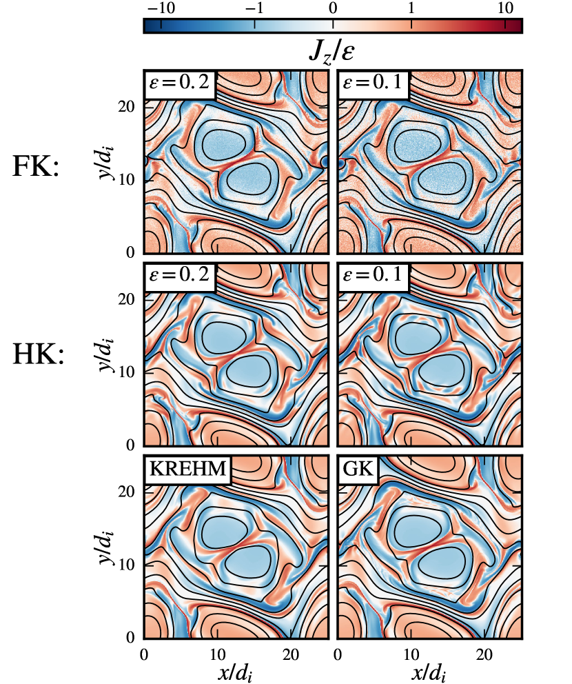
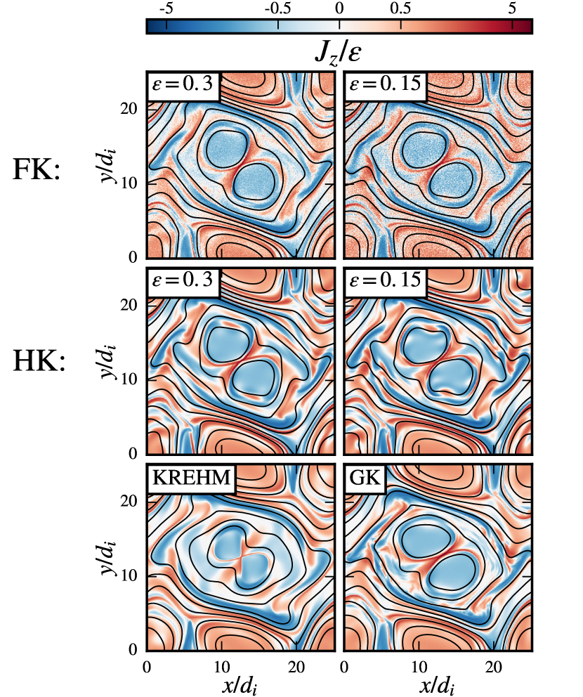
Figure 1: Contour plots of $J_{z}$ for $\beta_{i}=0.1$ (left) and $\beta_{i}=0.5$ (right). A doubly-logarithmic color scale (one for positive and one for negative values, with a narrow linear scale around 0 to connect the two) is used here to reveal also the fluctuations of weaker intensity. The color range has been adjusted according to the maximum value for any data set.

In Table 2 we list the root-mean-square values of the out-of-plane current density at 4.7 eddy turnover times. Short-time averaged data is used here to compute the root-mean-square values for the FK model in order to reduce contributions from the background PIC noise. While the spatial field structures are overall in good qualitative agreement, the root-mean-square current numerical values differ. More specifically, the numerical values deviate from the FK model up to 9% for GK, up to 12% for KREHM, and up to 33% for the HK model. We note that minor deviations can occur not only as a result of physical differences but also due to differences in the numerical grid size and low-pass filters, as well as due to PIC noise in the FK runs that may slightly affect the small-scale dynamics. On the other hand, regarding the relatively large disagreement between the HK and FK models, it is reasonable to assume that the main cause for the difference are electron kinetic effects absent in the HK approximation. To support the claim, we consider in Fig. 2 the root-mean-square values of the low-pass filtered electric current, $J_{z}^{\rm rms}(k_{\perp}\leq K)$, plotted versus the cutoff wavenumber $K$. A significant difference between the HK and FK results for $J_{z}^{\rm rms}$ is generated over the range of scales $1/\rho_{i}\lesssim k_{\perp}\lesssim 1/d_{e}$, over which the HK turbulent spectra are likely shallower due to the absence of electron Landau damping as demonstrated in Sec. 4.3.

$J_{z}^{\rm rms}/\epsilon$
	$\beta_{i}=0.1$		$\beta_{i}=0.5$
	$\epsilon=0.2$	$\epsilon=0.1$	$\epsilon=0.3$	$\epsilon=0.15$
FK	1.09	1.24	0.85	0.93
HK	1.31	1.44	1.08	1.24
GK	1.13		0.91
KREHM	1.12		0.82

Table 2: Comparison of the root-mean-square values of $J_{z}/\epsilon$ around 4.7 eddy turnover times in the simulation.

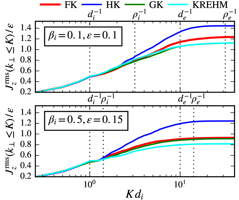
Figure 2: Comparison of the root-mean-square values of the low-pass filtered $J_{z}$, plotted against the cutoff wavenumber $K$.

In agreement with previous works (see review by Matthaeus et al. (2015) and references therein), the snapshots of $J_{z}$ in Fig. 1 also reveal a hierarchy of current sheets which differentiate with respect to the background Gaussian fluctuations, leading to scale-dependent statistics also known as intermittency. To investigate intermittency in our simulations, we study the statistics of magnetic field increments $\Delta_{x}B_{y}({{\ell}})=B_{y}(\mathbf{r}\nobreak+\nobreak{{\ell}\,\hat{\mathbf{e}}_{x}})-B_{y}(\mathbf{r})$, using the $B_{y}$ component and with spatial displacements $\ell$ along the (positive) $x$ direction. In Figure 3, we compare the probability distribution functions (PDFs) of magnetic field increments for the $\beta_{i}=0.1$ runs. The PDFs are computed as normalized histograms of $\Delta_{x}B_{y}({{\ell}})$ with equally spaced bins, using raw simulation data for the FK model. We also confirmed that the PDFs of $\Delta_{x}B_{y}({{\ell}})$ change only very little upon replacing the raw FK PIC data with short-time averaged data (not shown here). To smooth out the statistical fluctuations in the PDFs during the turbulent decay, we average the PDFs over a time window from roughly 4.4 to 5 eddy turnover times, when the turbulence is already well developed. The departure from a Gaussian PDF (black dashed lines in Fig. 3) increases from large to small scales. Good agreement is found between all models, except for very large values at the tails of the PDFs. Here we point out that the tails of the PDFs are likely to be affected by the differences in the smallest resolved scale in each model, which depends on the numerical resolution. Even though the level of intermittency in our simulations, compared to the solar wind, is likely underestimated due to a limited system size, the analysis shows that the turbulent fields still maintain a certain degree of intermittency, which does not appear to be particularly sensitive to different types of reduced-kinetic approximations. Our results are also in qualitative agreement with some observational studies and kinetic simulations (Leonardis et al., 2013; Wu et al., 2013b; Franci et al., 2015; Leonardis et al., 2016), even though it should be mentioned that some contradictory results have been reported based on observational data (Kiyani et al., 2009; Chen et al., 2014), for which the authors found non-Gaussian but scale-independent PDFs at kinetic scales.

To compare the level of intermittency in detail, we also compute the scale-dependent flatness, $K(\ell)=\langle\Delta_{x}B_{y}(\ell)^{4}\rangle/\langle\Delta_{x}B_{y}(\ell)^{2}\rangle^{2}$, of magnetic field fluctuations (Fig. 4), where $\langle\dots\rangle$ represents a space average. Similar to the PDFs, we additionally average $K(\ell)$ over a time window from 4.4 to 5 eddy turnover times. The flatness is close to the Gaussian value of 3 (black dashed lines in Fig. 4) at large scales and increases well above the $K=3$ threshold at kinetic scales. Furthermore, Fig. 4 also shows that the small-scale intermittency is somewhat underestimated in the HK and KREHM simulations. As already pointed out, intermittent properties can be very sensitive to the choice of numerical resolution, which might be responsible for the lower level of intermittency in the HK simulations. In particular, the HK flatness is closer to the FK and GK ones for the $\beta_{i}=0.5$ run, for which the smallest relevant scale of the FK and GK models ($\rho_{e}$) is closer to the limits of the HK resolution than in the $\beta_{i}=0.1$ case. Further investigations will be necessary to establish a thorough understanding of kinetic-scale intermittency with respect to different types of reduced-kinetic approximations. The need to perform a detailed study of intermittency with emphasis on kinetic model comparison has already been recognized by several authors and a detailed plan to fulfil this (among others) ambitious goal has been recently outlined in the so-called “Turbulent dissipation challenge” (Parashar et al., 2015b).

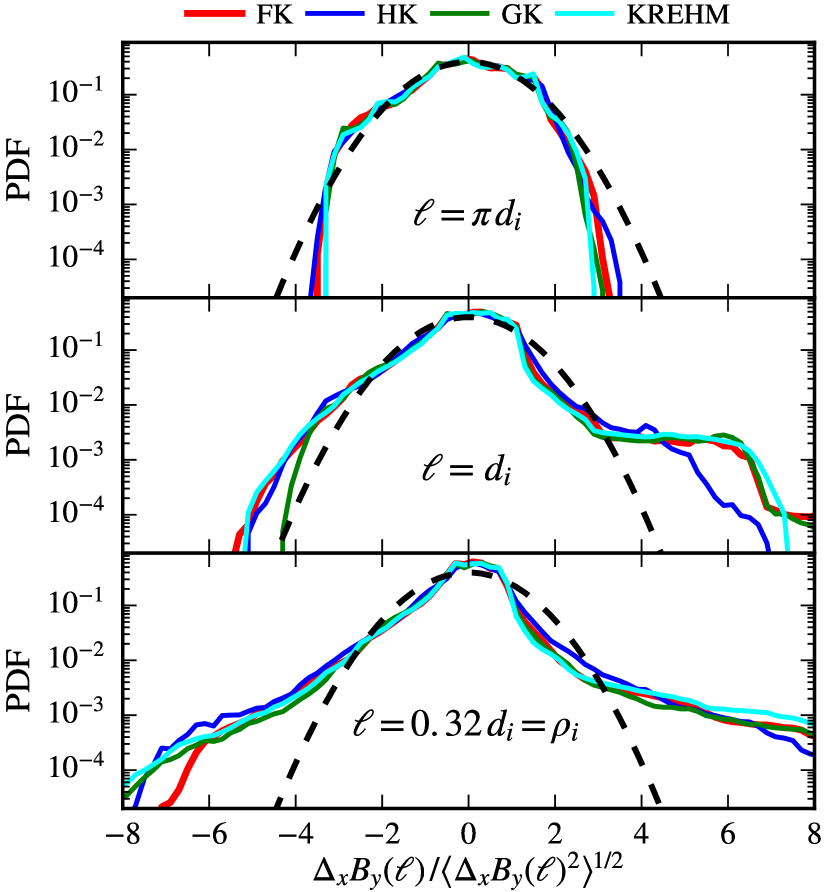
Figure 3: PDFs of magnetic field increments for different separation lengths $\ell$. The data is shown for the $\beta_{i}=0.1$ case with $\epsilon=0.1$ for the FK and HK models. The black dashed line corresponds to the (normalized) Gaussian PDF.

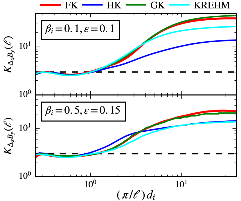
Figure 4: Scale-dependent flatness of perpendicular magnetic field increments for $\beta_{i}=0.1$ (top) and $\beta_{i}=0.5$ (bottom).

4.2 Global time evolution

Next, we consider the global turbulence energy budget of the decaying Orszag-Tang vortex. For this purpose, we split the bulk energy into magnetic $M=\langle B^{2}/8\pi\rangle$, kinetic ion $K_{i}=\langle nm_{i}u_{i}^{2}/2\rangle$, kinetic electron $K_{e}=\langle nm_{e}u_{e}^{2}/2\rangle$, internal ion $I_{i}=\langle 3nT_{i}/2\rangle$, and internal electron $I_{e}=\langle 3nT_{e}/2\rangle$ energy density, where $\langle\dots\rangle$ denotes a space average. To measure the energy fluctuations occurring as a result of turbulent interactions, we consider only the relative changes for each energy channel, normalized to the sum of the initial magnetic and kinetic ion energy density, $E_{0}=M(t=0)+K_{i}(t=0)$. The time traces for the FK model are obtained by space-averaging the raw simulation data without the use of short-time averaged fields. For the GK model and KREHM, we define the perturbed internal energy similar to Li et al. (2016) as

$$\delta I_{s}=-T_{0,s}\delta S_{s}-\delta K_{s}+\int_{0}^{t}{\mathcal{D}_{s}}\,\mathrm{d}t^{\prime},$$ (21)

where $\delta S_{s}=-\frac{1}{V}\int\,\mathrm{d}^{2}\mathbf{r}\,\mathrm{d}^{3}\mathbf{v}\delta f_{s}^{2}/2F_{0,s}$ is the perturbed species entropy and ${\mathcal{D}}_{s}$ is the mean species dissipation rate, occurring as a result of (hyper)collisional and (hyper)diffusive terms in the equations. The first two terms on the right-hand side correspond to free energy fluctuations without contributions from bulk fluid motions. The last term represents the amount of dissipated free energy of species $s$. In full $f$ models, the “dissipated” nonthermal energy stemming from (numerical) collisional effects in velocity space remains part of the distribution function in the form of thermal fluctuations. On the other hand, in $\delta f$ models such as GK and KREHM the thermalized energy is not accounted for in the background distribution $F_{0,s}$ and has to be added explicitly to the internal energy expression. The dissipative term is significant for both ions and electrons. In the GK simulations, hypercollisionality contributes to around 56% and 67% of $\delta I_{e}$ and to about 5% and 14% of $\delta I_{i}$ at $t\approx 6.3\tau_{0}$ for $\beta_{i}=0.1$ and $\beta_{i}=0.5$, respectively.

The time traces of the mean energy densities are shown in Fig. 5. The observed deviations from the FK curves appear to be consistent with the kinetic approximations made in each of the other three models. In particular, the HK model exhibits an excess of magnetic and electron kinetic energy density, which can be understood in the context of the isothermal electron closure that prevents turbulent energy dissipation via the electron channel. For the GK model, the result shows that GK tends to overestimate the electron internal energy and underestimate the ion one, with the deviations from the FK model growing as $\epsilon$ is increased. The observed amplification of ion internal energy relative to the electron one when $\epsilon$ is increased is also in good agreement with previous FK studies (Wu et al., 2013a; Matthaeus et al., 2016; Gary et al., 2016). The convergence of the FK internal energies towards the GK result as $\epsilon\to 0$ is consistent with the low $\epsilon$ assumption made in the derivation of the GK equations. Similarly, the improved agreement of KREHM with the FK model for the lower beta ($\beta_{i}=0.1$) runs can be understood in the context of the low beta assumption made in KREHM. We also note that ion heating is ordered out of the KREHM equations, which appears to be reasonable given the fact that the ion internal energy increases more rapidly in the higher beta ($\beta_{i}=0.5$) run.

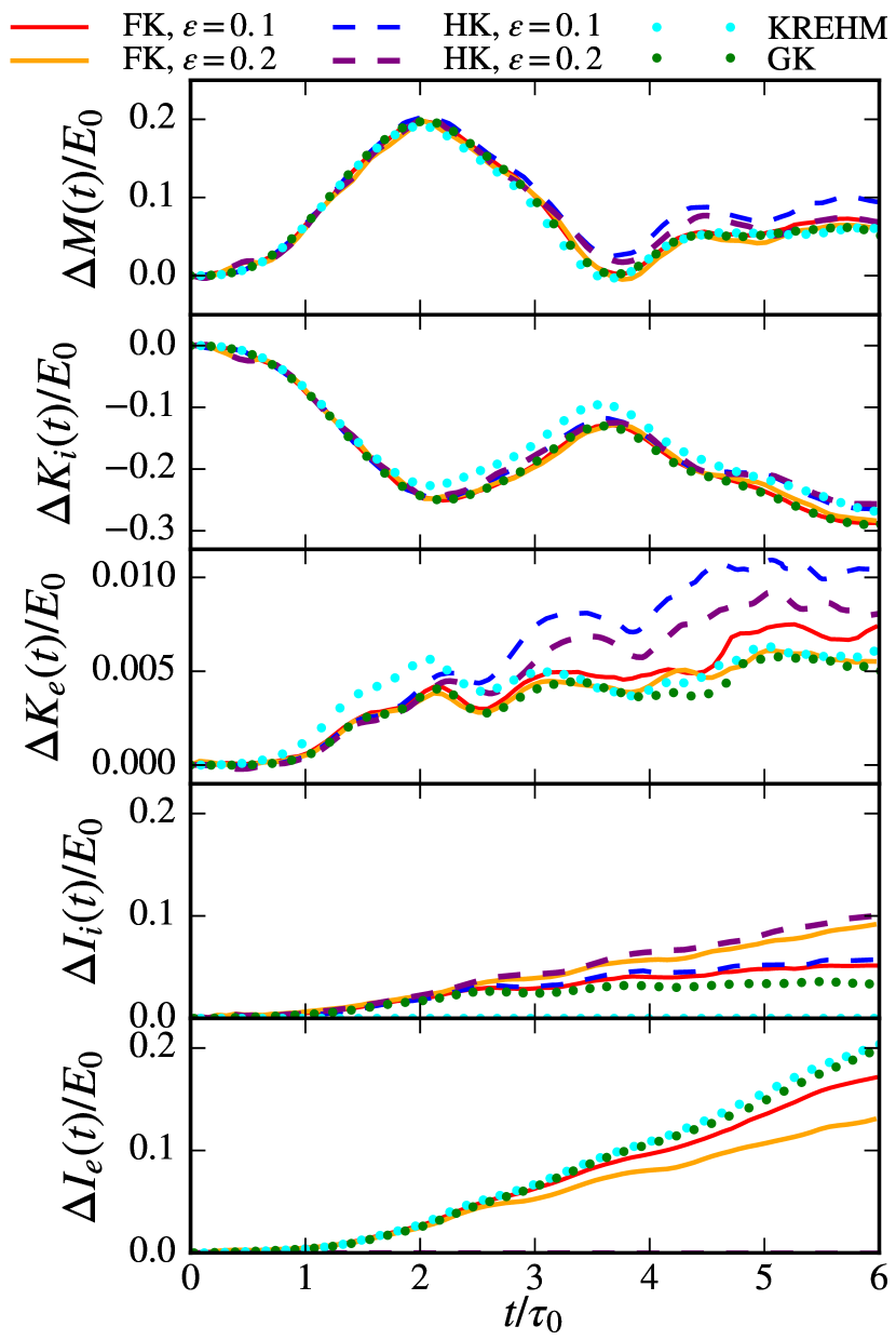
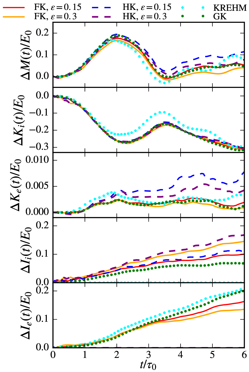
Figure 5: Global energy time traces for $\beta_{i}=0.1$ (left) and $\beta_{i}=0.5$ (right). Shown from top to bottom are the relative changes in the magnetic, kinetic ion, kinetic electron, internal ion, and internal electron energy densities. All quantities are normalized to the initial turbulent energy $E_{0}$, which we define as the sum of magnetic and ion kinetic energy density.

In summary, from the point of view of the global energy budget, all models deliver accurate results within the formal limits of their validity and in some cases even well beyond. The HK model resolves well ion kinetic effects but falls short in describing electron features, whereas the GK model becomes increasingly inaccurate for large turbulence fluctuation strengths. In addition to the $\epsilon\ll 1$ assumption of GK, the accuracy of KREHM also depends on the smallness of the plasma beta. For the particular setup considered, KREHM gives surprisingly good results already for $\beta_{i}=0.1$, which is well beyond its formal limit of validity ($\beta_{i}\lesssim 0.01$ for $m_{e}/m_{i}=0.01$ and $T_{0,i}=T_{0,e}$).

4.3 Spectral properties

The nature of the kinetic-scale, turbulent cascade is investigated by considering the one-dimensional (1D) turbulent spectra, which we compute as follows. We divide the two-dimensional perpendicular wavenumber plane $(k_{x},k_{y})$ into equally-spaced shells of width $\Delta k=k_{\min}=2\pi/L$ and calculate the 1D spectra, $P(k_{\perp})$, by summing the squared amplitudes of the Fourier modes contained in each shell. The wavenumber coordinates for the 1D spectra are assigned to the middle of each shell at integer values of $\Delta k$. To compensate for the global energy variations between different models (see Fig. 5) and to account for the fact that the turbulence is decaying, we normalize the spectra for each simulation and for each time separately, such that $\sum_{k_{\perp}}P(k_{\perp})=1$. Finally, we average the (normalized) spectral curves over a time interval from 4.4 to 5 eddy turnover times in order to smooth out the statistical fluctuations in $P(k_{\perp})$.

The turbulent spectra of the magnetic, perpendicular electric, and electron density fields are compared in Fig. 6. The spectra are shown for all simulation runs, using short-time averaged data for the FK model. For reference, we also plot the FK spectra obtained from the raw PIC data in the higher $\epsilon$ runs (A1 and B1 in Table 1). Since different numerical resolutions were used for different models, the scales at which (artificial) numerical effects become dominant differ between the models. For the HK model, it can be inferred from the spectrum that numerical effects due to low-pass filters (Lele, 1992) become dominant for $k_{\perp}\gtrsim 1/d_{e}$. On the other hand, for the FK, GK model, and KREHM, the physically well-resolved scales are roughly limited to $k_{\perp}\lesssim 1/\rho_{e}$. In the GK model and KREHM, the collisionless cascade is terminated by hyperdiffusive terms. In the FK runs, the main limiting factor are the background thermal fluctuations, which dominate over the collisionless turbulence at high $k_{\perp}$, as indicated by the grey shading in Fig. 6.

Two notable features stand out when comparing the spectra over the range of well-resolved scales. First, good agreement is seen between the FK and GK spectra, and secondly, the HK spectra have shallower spectral slopes at sub-ion scales. Under the assumptions made in the derivation of GK, the kinetic-scale, electromagnetic cascade can be understood in the context of kinetic Alfvén wave (KAW) turbulence—the nonlinear interaction among quasi-perpendicularly propagating KAW packets (Howes et al., 2008a; Schekochihin et al., 2009; Boldyrev et al., 2013). Thus, the comparison between the GK and FK turbulent spectra suggests a predominantly KAW type of turbulent cascade between ion and electron scales without major modifications due to physics not included in GK, such as ion cyclotron resonance (Li & Habbal, 2001; Markovskii et al., 2006; He et al., 2015), high frequency waves (Gary & Borovsky, 2004; Gary & Smith, 2009; Verscharen et al., 2012; Podesta, 2012), and large fluctuations in the ion and electron distribution functions. We emphasize here that our results are, strictly speaking, valid only for the particular setup considered and could be modified in three-dimensional geometry and/or for a realistic value of the ion-electron mass ratio. Concerning the HK results, the shallower slopes can be regarded as manifest for the influence of electron kinetic physics on the sub-ion-scale turbulent spectra. In particular, several previous works demonstrated that electron Landau damping could be significant even at ion scales of the solar wind (Howes et al., 2008a; TenBarge & Howes, 2013; Told et al., 2015, 2016b; Bañón Navarro et al., 2016), and therefore, we explore this aspect further in what follows.

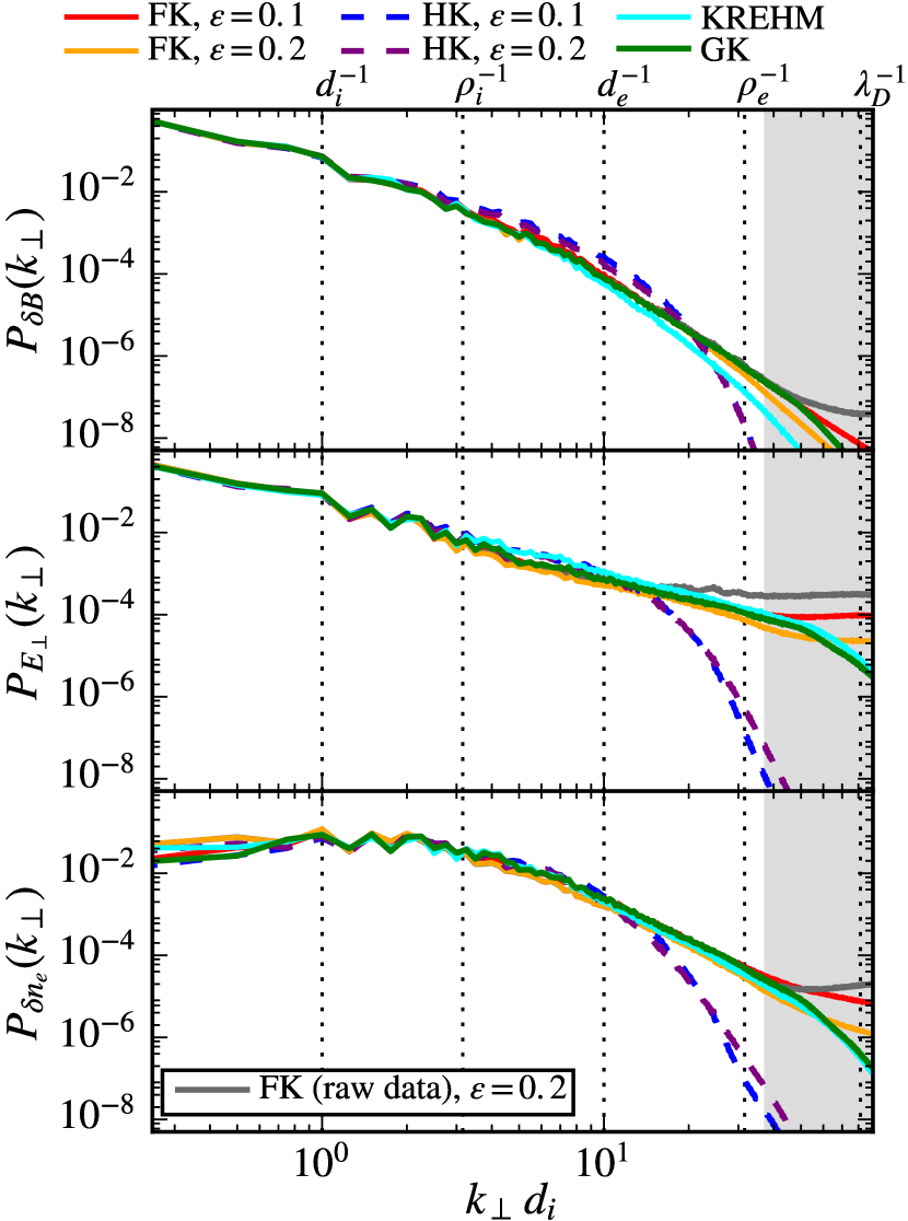
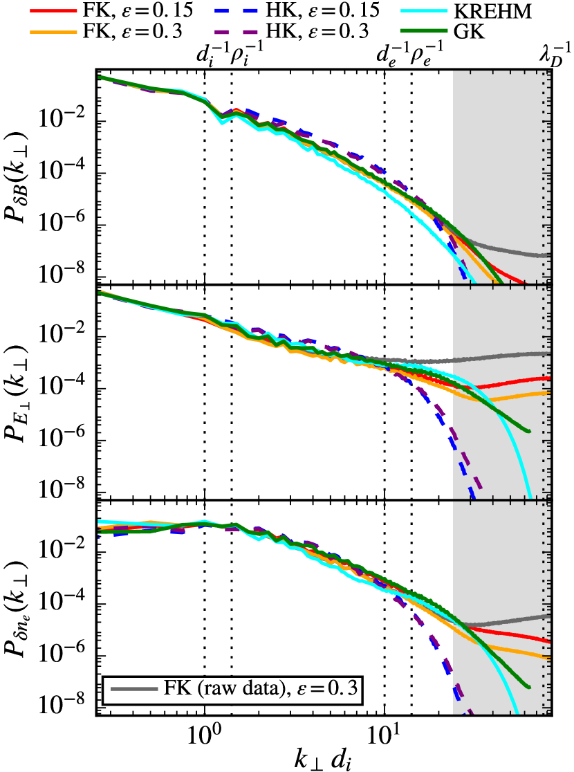
Figure 6: One-dimensional $k_{\perp}$ energy spectra for $\beta_{i}=0.1$ (left) and $\beta_{i}=0.5$ (right). Shown from top to bottom are the $\delta\mathbf{B}$ spectra, the $\mathbf{E}_{\perp}$ spectra, and the electron density spectra. The grey-shaded regions indicate the range where PIC noise dominates over the turbulent fluctuations for the short-time averaged fully kinetic PIC data. The grey lines show the FK spectra for the raw data.

The role of electron Landau damping is investigated with KREHM, for which electron Landau damping is the only process leading to irreversible heating. All other dissipation channels are ordered out as a result of the low $\beta$ and low $\epsilon$ limit (Zocco & Schekochihin, 2011). To test the influence of electron heating on the KREHM spectra, we performed a new set of simulations in the isothermal electron limit with $g_{e}$ in Eq. (13) set equal to $g_{e}=0$. In Figure 7 we compare the FK and HK magnetic field spectra with the KREHM spectra obtained from simulations with and without electron heating. Only the curves corresponding to the low $\epsilon$ runs (A2 and B2) are shown for the FK and HK models. Over the range of scales where numerical dissipation in the HK runs is negligible ($k_{\perp}\lesssim 1/d_{e}$), excellent agreement between the isothermal KREHM spectra and the HK spectra is found for the $\beta_{i}=0.1$ case. On the other hand, when the isothermal electron assumption is relaxed, the KREHM result is much closer to the FK than to the HK spectrum. A similar trend can be inferred for the $\beta_{i}=0.5$ regime, albeit with some degradation in the accuracy of KREHM, which is to be expected given its low $\beta$ assumption. Furthermore, to demonstrate that electron heating indeed leads to small-scale parallel velocity space structures, reminiscent of (linear) Landau damping, we compute the Hermite energy spectrum of $g_{e}$ (Schekochihin et al., 2009; Zocco & Schekochihin, 2011; Loureiro et al., 2013; Hatch et al., 2014; Schekochihin et al., 2016), which is shown Fig. 8. The Hermite energy spectrum can be regarded as a decomposition of the free energy among parallel velocity scales (the higher the Hermite mode number $m$, the smaller the parallel velocity scale). Due to a limited number of Hermite polynomials used in the KREHM simulations ($M=30$), no clean spectral slope can be observed. However, over a limited range of scales ($m\lesssim 7$), the Hermite spectrum is shallow and suggests a tendency towards the asymptotic limit $\sim m^{-1/2}$ predicted for linear phase mixing, i.e. Landau damping (Zocco & Schekochihin, 2011). We also mention that a recent three-dimensional study of the turbulent decay of the Orszag-Tang vortex demonstrated a clear convergence towards the $m^{-1/2}$ limit for much larger sizes of the Hermite basis (up to $M=100$), thus indicating a certain robustness of the result (Fazendeiro & Loureiro, 2015).

Finally, the importance of electron Landau damping at sub-ion scales might be somewhat overestimated in our study due to the use of a reduced ion-electron mass ratio of 100, resulting in a $\sim 4.3$ times smaller scale separation between ion and electron scales (compared to a real hydrogen plasma). In this work, no definitive answer concerning the role of the reduced mass ratio can be given and further investigations with higher mass ratios will be needed to clarify this aspect. We note, however, that a recent GK study of KAW turbulence, as well as a comparative study of linear wave physics contained in the FK, HK, and GK model found that electron Landau damping at ion and sub-ion scales can be relevant even for a realistic mass ratio (Told et al., 2016b; Bañón Navarro et al., 2016). We also mention that, in principle, one should not overlook the fact that electron Landau damping is absent in the HK model not only for KAWs but for all other waves as well, such as the fast/whistler, slow, and ion Bernstein modes.

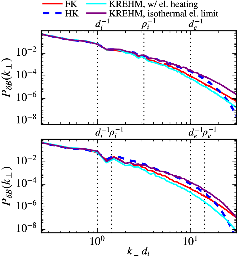
Figure 7: Comparison of the FK, HK, and KREHM magnetic field spectra with the isothermal electron limit of KREHM for $\beta_{i}=0.1$ (top) and $\beta_{i}=0.5$ (bottom).

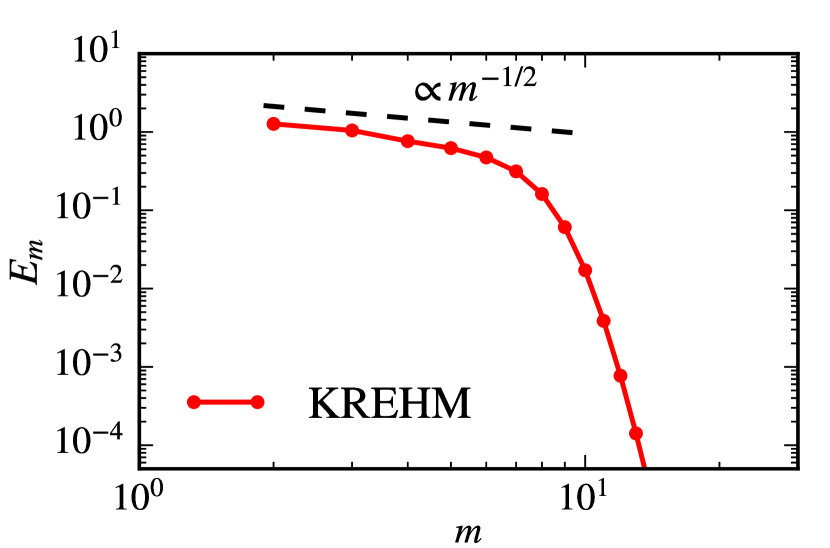
Figure 8: Hermite spectrum of the electron free energy, obtained from the KREHM simulation corresponding to the $\beta_{i}=0.1$ set of runs. The $m^{-1/2}$ slope is shown for reference.

To compare the spectral properties of the solutions in even greater detail, we examine the ratios of the 1D $k_{\perp}$ spectra (Gary & Smith, 2009; Boldyrev et al., 2013; Salem et al., 2012; Chen et al., 2013; Franci et al., 2015; Cerri et al., 2016). The ratios are often considered in literature as a diagnostic for distinguishing different types of wave-like properties (e.g. KAWs versus whistler waves). We emphasize that the reference to wave physics should not be considered as an attempt of demonstrating the dominance of linear dynamics over the nonlinear interactions. Instead, the motivation for considering linear properties should be associated with the conjecture of critical balance (Goldreich & Sridhar, 1995; Howes et al., 2008a; Cho & Lazarian, 2009; TenBarge & Howes, 2012; Boldyrev et al., 2013), which allows for strong nonlinear interactions while still preserving certain properties of the underlying wave physics. It is also worth mentioning that a nonzero parallel wavenumber $k_{\parallel}$ along the magnetic field is required for the existence of many types of waves (such as KAWs), relevant for the solar wind. Wavenumbers with $|k_{z}|>0$ along the direction of the mean field are prohibited in our simulations due to the two-dimensional geometry adopted in this work. While $k_{z}=0$, the magnetic fluctuations $\delta B_{K_{\perp}}^{<}$ above some reference scale $\ell_{0}\sim 1/K_{\perp}$ may act as a local guide field on the smaller scales ($\ell\sim 1/k_{\perp}<\ell_{0}$), giving rise to an effective parallel wavenumber $k_{\parallel}\sim\mathbf{k}_{\perp}\cdot\delta\mathbf{B}_{K_{\perp}}^{<}/B_{0}$ (Howes et al., 2008a; Cerri et al., 2016; Li et al., 2016). In this way, certain wave properties may survive even in two-dimensional geometry, even though a fully three-dimensional study would surely provide a greater level of physical realism.

Four different ratios of the 1D spectra are considered:

$$C_{A} =|E_{\perp}|^{2}/|\delta B_{\perp}|^{2}, C_{p} =\beta_{i}^{2}\,|\delta n_{e}|^{2}/|\delta B_{z}|^{2},$$

$$C_{e} =|\delta n_{e}|^{2}/|\delta B|^{2}, C_{\parallel} =|\delta B_{z}|^{2}/|\delta B|^{2},$$

where $C_{e}$ and $C_{\parallel}$ are known as the electron and magnetic compressibility, respectively. Large scale Alfvénic fluctuations have $C_{A}\sim 1$, whereas $C_{p}\sim 1$ implies a balance between the perpendicular kinetic and magnetic pressures. In the asymptotic limit $1/\rho_{i}\ll k_{\perp}\ll 1/\rho_{e}$, the ratios for KAW fluctuations are expected to behave as $C_{A}\sim(k_{\perp}\rho_{i})^{2}/(4+4\beta_{i})$, $C_{e}\sim 1/(\beta_{i}+2\beta_{i}^{2})$, $C_{\parallel}\sim\beta_{i}/(1+2\beta_{i})$, and $C_{p}\sim 1$, assuming $k_{\perp}\gg k_{\parallel}$, singly charged ions, and $T_{0,i}=T_{0,e}$ (Schekochihin et al., 2009; Boldyrev et al., 2013). Thus, the $C_{A}$ ratio is expected to grow with $k_{\perp}$, while the other three ratios are in the first approximation roughly independent of $k_{\perp}$ on sub-ion scales. In the regime $\beta_{i}\lesssim 1$ relevant to this work, we also expect $C_{e}\gtrsim C_{\parallel}$.

The spectral ratios are compared in Fig. 9. Focusing first on the range of scales $1/\rho_{i}\lesssim k_{\perp}\lesssim 1/\rho_{e}$, we find good agreement between the GK and FK models, albeit with moderate disagreements between the $C_{p}$ ratios in the $\beta_{i}=0.1$ regime. Thus, the ratios provide firm evidence for a KAW cascade scenario for $\beta_{i}=0.5$, whereas for $\beta_{i}=0.1$, even though apparently dominated by KAW fluctuations, the cascade is also influenced by phenomena excluded in GK. Considering the large-scale dynamics in the $k_{\perp}\lesssim 1/\rho_{i}$ range, very good agreement is found between the FK and HK results, whereas the GK $C_{e}$, $C_{p}$, and $C_{\parallel}$ ratios significantly deviate. It is worth noticing that the $C_{p}$ ratio depends only on the magnetic fluctuations parallel to the mean field $\delta B_{z}$, which represent a fraction of the total magnetic energy content as evident from the results for $C_{\parallel}$.

The general trends exhibited by the FK and HK ratios seem to suggest the presence of high frequency waves (e.g. fast magnetosonic modes) excluded in GK. To check if the FK and HK solutions in the $k_{\perp}\lesssim 1/\rho_{i}$ range (and even beyond for $\beta_{i}=0.1$) are indeed consistent with a mixture of modes present (KAWs, slow modes, entropy modes) and excluded (e.g. fast modes) in GK, we numerically solve the HK dispersion relation in the $\beta_{i}=0.1$ regime using a recently developed HK dispersion relation solver (Told et al., 2016a). The qualitative findings discussed below for $\beta_{i}=0.1$ can be also applied to the $\beta_{i}=0.5$ case (not shown here).

A collection of least damped modes identified with the HK linear dispersion relation solver is shown in Fig. 10. Two fixed propagation angles with respect to the magnetic field are considered; 89 and 85 degrees. The identified branches can be interpreted as KAWs, fast modes, and generalized ion Bernstein modes. For the sake of simplicity, we do not consider slow modes and entropy modes because our goal here is to study the properties of waves excluded in GK [for a detailed discussion on GK wave physics see Howes et al. (2006)]. The identified ion Bernstein modes are generalized in the sense that they are not purely perpendicularly propagating nor electrostatic and they also split into multiple branches around the cyclotron frequency. As pointed out by Podesta (2012), the fine splitting of the ion Bernstein modes may increase the opportunity for wave coupling with the fast and KAW branch.

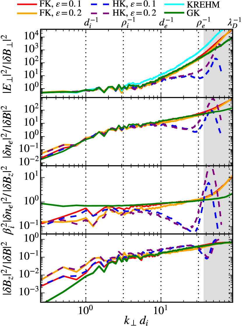
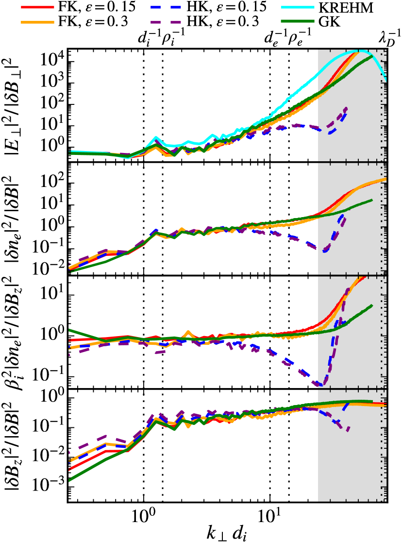
Figure 9: Ratios of the one-dimensional turbulent spectra. The left panel shows the ratios for the $\beta_{i}=0.1$ runs and the right panel shows the ratios for $\beta_{i}=0.5$. The grey-shaded regions indicate the range of scales dominated by PIC noise in the FK simulations.

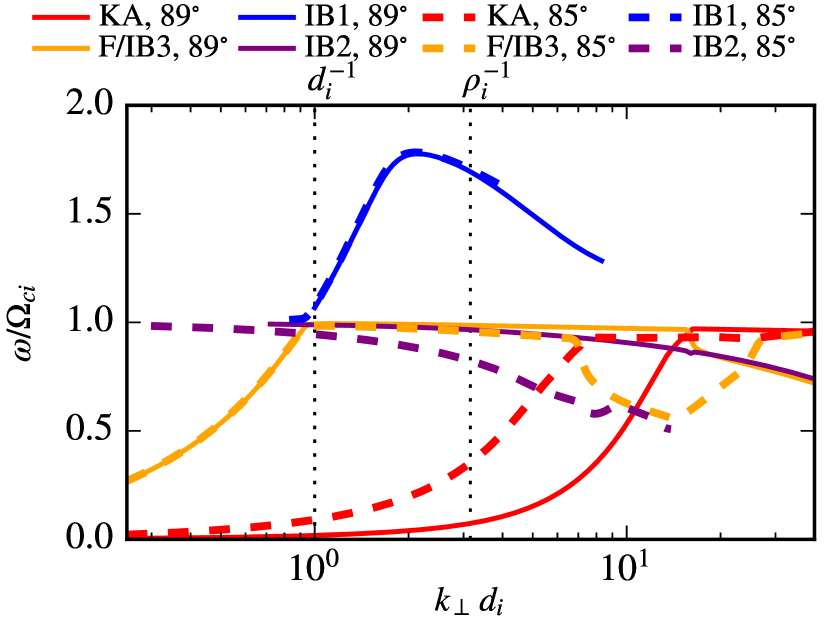
Figure 10: Numerical solutions of the hybrid-kinetic dispersion relation for $\beta_{i}=0.1$. The labels KA, F, and IB are used to denote kinetic Alfvén waves, fast waves, and (different branches of) ion Bernstein modes, respectively.

Having identified the main branches of interest, we now proceed to show the corresponding spectral ratios (Fig. 11). In addition to the spectral ratios obtained from the HK solver, we also show for reference the GK prediction for the spectral ratios of KAWs (using $m_{i}/m_{e}=100$), as well as the linear damping rates of the HK branches. Comparing the linear predictions with the turbulent ratios shown in the left panel of Fig. 9, we find that the directions in which the FK and HK turbulent ratios are “pulled away” from the GK curves are consistent with linear properties of fast and ion Bernstein modes. In particular, the magnetic compressibility $C_{\parallel}$ is order unity for the fast and ion Bernstein modes, whereas their $C_{p}$ ratio is below the pressure balance regime $C_{p}\sim 1$. Similarly, the electron compressibility $C_{e}$ exceeds the one of KAWs at low wavenumbers. All these properties are in qualitative agreement with the general trends exhibited by the FK and HK turbulent solutions for $k_{\perp}\lesssim 1/\rho_{i}$. Regarding the $C_{A}$ ratio, we note that $\delta B_{\perp}/\delta B\ll 1$ for the fast and ion Bernstein modes, meaning that these modes cannot significantly influence the total $|E_{\perp}|^{2}/|\delta B_{\perp}|^{2}$ ratio when mixed together with the Alfvénic fluctuations. Looking at the damping rates, linear theory predicts cyclotron damping of the fast mode already at $k_{\perp}\sim 1/d_{i}$. However, the GK turbulent ratios deviate from the FK model beyond the $k_{\perp}\sim 1/d_{i}$ scale for $\beta_{i}=0.1$. Therefore, the coupling of the fast modes to the ion Bernstein modes is likely significant in the low-beta regime. The most natural candidate for the conversion of the fast wave would be the mode denoted as IB1 in Fig. 10, which is very weakly damped in the HK model and allows for a continuation of the fast branch above the ion cyclotron frequency. In the FK model, ion Bernstein waves are subject to additional damping due to electron Landau resonance which could potentially explain why all the FK ratios show a tendency for converging onto the GK curves with increasing wavenumbers, whereas in the HK model, the turbulent ratios (in particular $C_{p}$ and $C_{\parallel}$) do not share the same trend.

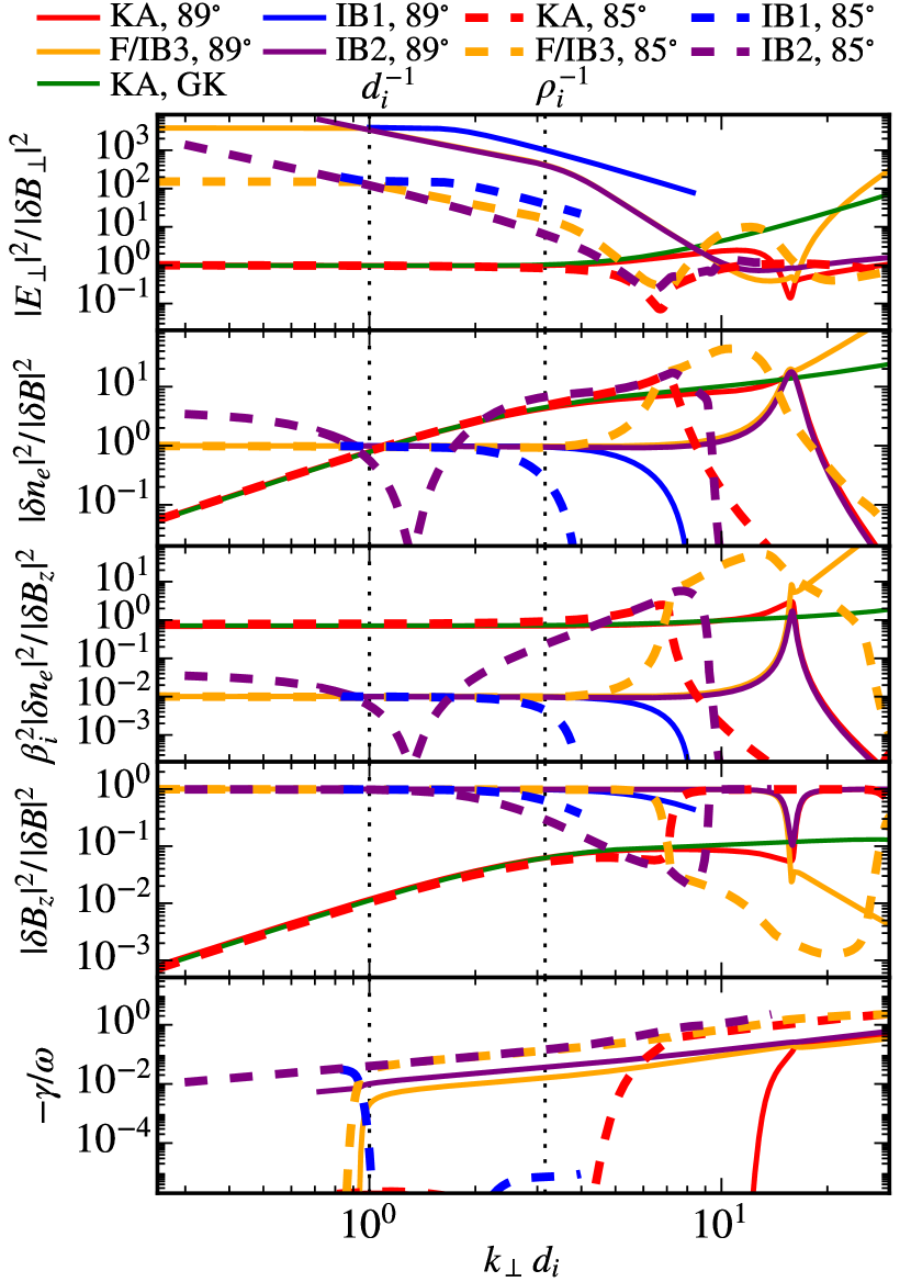
Figure 11: Spectral ratios corresponding to different solutions of the HK dispersion relation (top four plots) and their linear damping rates (bottom). For reference, we also show the GK prediction for the spectral ratios of KAWs.

In summary, we conclude that the deviation of the GK model from the FK and HK turbulent solutions in the range $k_{\perp}\lesssim 1/\rho_{i}$, and possibly even beyond for $\beta_{i}=0.1$, can be reasonably well explained with the presence of fast magnetosonic and ion Bernstein modes, coexisting together with Alfvénic fluctuations. On the other hand, we admit that alternative explanations involving, for example, non-wave-like phenomena could be in principle possible. As a side note, it is also worth mentioning that according to linear theory, KAWs should undergo cyclotron resonance around $k_{\perp}d_{i}\sim 10$ (see bottom plot in Fig. 11), resulting in an abrupt change in the spectral ratios. No such variation is found in the FK turbulent ratios. This suggests that cyclotron resonance has in our case only a minor effect on the turbulent cascade, in consistency with the arguments against cyclotron resonance given by Howes et al. (2008a).

4.4 Ion and electron nonthermal free energy fluctuations

At last, motivated by previous works on non-Maxwellian velocity structures in HK simulations (Greco et al., 2012; Valentini et al., 2014; Servidio et al., 2015) and free energy cascades in GK and KREHM (Schekochihin et al., 2009; Bañón Navarro et al., 2011; Zocco & Schekochihin, 2011; Told et al., 2015; Schekochihin et al., 2016), we investigate the spatial distribution of the nonthermal species free energy fluctuations:

$$\delta\tilde{\mathcal{E}}_{s}=\int\frac{T_{0,s}\delta\tilde{f}_{s}^{2}}{2F_{0,s}}\,\mathrm{d}^{3}\mathbf{v},$$ (22)

where $\delta\tilde{f}_{s}$ is the perturbed part of the distribution function with vanishing lowest three moments (density, fluid velocity, and temperature), $T_{0,s}$ is the equilibrium temperature, and $F_{0,s}$ is the background Maxwellian. Expression (22) can be regarded as a measure for quantifying the deviations from local thermodynamic equilibrium, characterized by non-Maxwellian fluctuations in velocity space that set the stage for irreversible plasma heating to occur. Due to a limited availability of data and refined diagnostic tools, needed for the calculation of the nonthermal free energy as a function of space, we present here only the results from a subset of all simulations and models. In particular, we focus on the $\beta_{i}=0.1$ regime and consider the ion nonthermal fluctuations calculated from the HK model and the electron nonthermal fluctuations calculated from the $v_{\perp}$-integrated distribution functions in the FK model and KREHM. In the HK and FK models, we define $\delta\tilde{f}_{s}$ as $\delta\tilde{f}_{s}=f_{s}-F_{0,s}$, where $F_{0,s}$ is the local Maxwellian with matching density, fluid velocity, and temperatures of the total distribution $f_{s}$. In KREHM, the equivalent of expression (22) can be defined as $\delta\tilde{\mathcal{E}}_{\parallel,e}=n_{0}T_{0,e}\sum_{m=3}^{M}\hat{g}_{m}^{2}/2$, where $\hat{g}_{m}$ are the Hermite expansion coefficients of $g_{e}$ (Zocco & Schekochihin, 2011; Schekochihin et al., 2016). By skipping the lowest three coefficients ($m\leq 2$) in the above sum, the contributions from density, fluid velocity, and temperature fluctuations are explicitly excluded from the KREHM free energy. Here, we only consider parallel electron velocity fluctuations because $g_{e}$ does not depend on $v_{\perp}$ in KREHM. For the FK model, on the other hand, the $v_{\perp}$-integrated electron distribution function is used as a necessity, due to a limitation in diagnostic tools presently available for the FK PIC code used in this work. The limitation to parallel velocity fluctuations is, however, physically well-motivated for the electrons based on a number of previous works, which showed that electron heating takes place predominantly in the parallel direction (Saito et al., 2008; TenBarge & Howes, 2013; Haynes et al., 2014; Numata & Loureiro, 2015; Li et al., 2016; Bañón Navarro et al., 2016).

The nonthermal ion and electron free energy fluctuations are shown in Fig. 12. The snapshots correspond to the $\beta_{i}=0.1$ runs around 4.7 eddy turnover times, with $\epsilon=0.2$ in the HK and FK simulations. For reference, we also show in Fig. 13 the corresponding ion and electron temperature fluctuations $\delta T_{s}=T_{s}-\langle T_{s}\rangle$, plotted at same time in the HK and FK simulation. A highly nonuniform spatial distribution of the nonthermal free energy is found for both ions and electrons. Furthermore, by overplotting the contours of the vector potential $A_{z}$ we find that the nonthermal fluctuations are mostly concentrated around small-scale magnetic reconnection sites, corresponding (in 2D) to the X-points of $A_{z}$. Fig. 12 also shows some disagreements in the nonthermal free energy spatial profiles between the FK model and KREHM. Considering the abovementioned circumstances, one could suppose that the disagreements are related to the small-scale differences in magnetic field configuration, which might consequently impact the exact locations where reconnection is taking place. A detailed investigation of the possible causes for the observed disagreements is beyond the scope of this study but could be carried out in future works.

The observed correlation between reconnection sites and nonthermal fluctuations is in good agreement with previous works (Greco et al., 2012; Valentini et al., 2014; Haynes et al., 2014; Servidio et al., 2015) and as such reinforces the idea that reconnection might play a significant role in the turbulent heating of kinetic-scale, collisionless plasma turbulence. Compared to Fig. 13, it is seen that the nonthermal free energy peaks are well correlated with temperature fluctuations, the main difference to the latter being that the nonthermal fluctuations are spatially more diffused. This seems to suggest that the energy supplied to the particles at reconnection sites is progressively cascaded to smaller velocity scales in the reconnection outflows, thus allowing the nonthermal fluctuations to spread over a larger volume compared to the temperature fluctuations. The generation of non-Maxwellian velocity space fluctuations can be, on the other hand, linked with the presence of wave-particle interactions such as Landau damping, as well as with kinetic instabilities (Haynes et al., 2014).

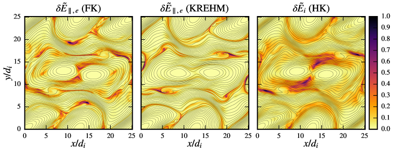
Figure 12: Nonthermal electron and ion free energy fluctuations. In the left and middle plots, we compare the FK and KREHM electron free energy, stemming from small scale structures in $v_{\parallel}$. The plot on the right shows the (total) nonthermal ion free energy obtained from the HK simulation. Overplotted are the contours of the vector potential $A_{z}$. The color map is normalized to the maximum value of the free energy, separately for each plot.

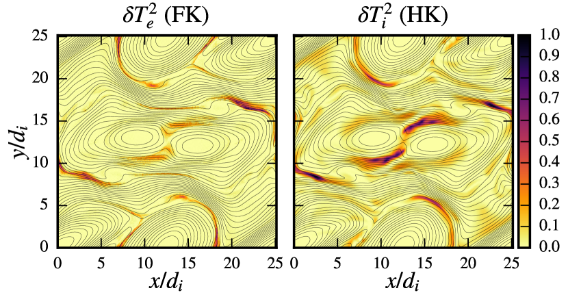
Figure 13: Ion and electron temperature fluctuations corresponding to the HK and FK nonthermal free energies shown in Fig. 12.

While the role of Landau damping in kinetic-scale, collisionless plasma turbulence is presently somewhat less known for the ions, the significance of electron Landau damping has been demonstrated in many previous studies (Howes et al., 2008a; TenBarge & Howes, 2013; Told et al., 2015; Bañón Navarro et al., 2016) and in Sec. 4.3 of this work. Conversely, we find—at the same time—that reconnection could as well be a major process leading to heating in collisionless plasma turbulence. Similar as for Landau damping, the latter idea is also well-supported by a number of previous studies (Sundkvist et al., 2007; Osman et al., 2011; Karimabadi et al., 2013; Chasapis et al., 2015; Matthaeus et al., 2015). Some of the previous works tried to establish a sharp distinction between heating due to wave-particle interactions versus heating occurring as a consequence of reconnection, often favouring one of the two possibilities as the main cause for turbulent heating. As one additional option, we would like to promote a rather different view, which is that these two seemingly distinct processes might work hand in hand and are spatially entangled with each other, making a clear distinction between heating due to Landau damping and reconnection a somewhat ill-posed task. Instead, it might be more instructive to consider these two processes in a unified framework and investigate, for example, how the (nonuniform) damping via Landau resonance might be affected by the presence of reconnection outflows, which could (locally) modify the Landau resonance condition. This view is supported by previous studies of weakly-collisional reconnection (Loureiro et al., 2013; Numata & Loureiro, 2015), and by a recent study of GK turbulence (Klein et al., 2017) which showed that, contrary to naive expectations, Landau damping in a turbulent setting can be spatially highly nonuniform and might be responsible for the intermittent heating observed in the vicinity of current sheets (Sundkvist et al., 2007; Osman et al., 2011; Wu et al., 2013b; Karimabadi et al., 2013; Chasapis et al., 2015). The possibility of a close relationship between reconnection and Landau damping was also implied in a recent study by Parashar & Matthaeus (2016), which mentioned a mechanism described as a nonlinear generalization of Landau resonance.

Finally, it is worth acknowledging one additional aspect of kinetic-scale reconnection, recently explored by Cerri & Califano (2017), Mallet et al. (2017), Loureiro & Boldyrev (2017), and Franci et al. (2017). In the abovementioned works, the authors argue that reconnection could also significantly impact the nonlinear energy transfer and the shape of the turbulent spectra at kinetic scales. This would consequently imply a more generalized type of kinetic cascade; one which is also influenced by non-local energy transfers (in spectral space) as opposed to local mode couplings in wave-like models of turbulence (Galtier & Bhattacharjee, 2003; Howes et al., 2008a; Schekochihin et al., 2009; Boldyrev et al., 2013; Passot & Sulem, 2015). A detailed investigation of this novel cascade phenomenology is beyond the scope of this work. Strictly speaking, the turbulent spectra and spectral ratios alone are not sufficient to unambiguously determine whether the energy transfer is local or not. Instead, the spectra and spectral ratios can only point out the dominant type of turbulent fluctuations at each wavenumber separately.

5 Conclusions

In this work, we performed a detailed comparison of kinetic models in two-dimensional, collisionless plasma turbulence with emphasis on kinetic-scale dynamics. Four distinct models were included in the comparison: the fully kinetic (FK), hybrid-kinetic (HK) with fluid electrons, gyrokinetic (GK), and a reduced gyrokinetic model, formally derived as a low beta limit of gyrokinetics (KREHM). Two different ion beta ($\beta_{i}$) regimes and variable turbulence fluctuation amplitudes ($\epsilon$) were considered ($\beta_{i}=0.1$ using $\epsilon=0.1,0.2$ and $\beta_{i}=0.5$ using $\epsilon=0.15,0.3$). The main findings can be summarized as follows:

• For $\beta_{i}=0.5$, the kinetic-scale ($k_{\perp}\gtrsim 1/d_{i}$) spectral properties of the FK and GK solutions were found to be in good agreement, thus suggesting a kinetic Alfvén cascade scenario from ion to electron scales without significant modifications due to physics not included in GK (Figs. 6 and 9).

• A detailed comparison between the GK and FK spectral ratios at $\beta_{i}=0.1$ reveals a deviation between the two models at kinetic scales (Fig. 9). However, given that the kinetic-scale ($k_{\perp}\gtrsim 1/d_{i}$) disagreement is clearly observed only for two out of four different spectral ratios considered, nor is it clearly seen in the turbulent spectra themselves (Fig. 6), it is reasonable to assume that kinetic Alfvén fluctuations still play a significant role even in the low-beta regime.

• At the largest scales ($k_{\perp}\lesssim 1/d_{i}$), the ratios of the GK turbulent spectra notably deviate from the FK and HK approaches for both ion betas (0.1 and 0.5), the likely cause for it being the lack of the fast magnetosonic modes in the GK approximation (Figs. 9, 10, and 11). The disagreement is larger for higher fluctuation amplitudes and for the lower value of the ion beta ($\beta_{i}=0.1$), for which the deviations carry over to kinetic scales, possibly via mode coupling to ion Bernstein waves.

• The sub-ion-scale HK spectra were found to be shallower than those obtained from the FK and GK simulations, presumably due to the lack of electron Landau damping (Figs. 6, 7, and 8).

• The real space turbulent field structures are in good qualitative agreement (Fig. 1). Furthermore, all models considered give rise to intermittent statistics at kinetic scales, albeit with some minor quantitative differences between the models (Figs. 3 and 4). The main reason for the observed deviations might be related to the fact that different numerical resolutions were used for different models. Further studies will be necessary to identify if the observed quantitative differences are indeed physical.

• The spatial profiles of the nonthermal ion and electron free energy fluctuations suggest that kinetic-scale reconnection might play an important role in the heating of the plasma (Figs. 12 and 13). Furthermore, our results also suggest that reconnection might be closely entangled with (nonuniform) Landau damping, making the distinction between heating due to reconnection versus heating due to Landau damping an ill-posed task.

• KREHM delivers surprisingly accurate results already for $\beta_{i}=0.1$, even though its range of validity is formally limited to $\beta_{i}\lesssim 0.01$ for our choice of the reduced mass ratio and equal ion and electron background temperatures (Figs. 1, 3, 4, 5, and 6).

We emphasize that, strictly speaking, our findings are valid only for the particular setup considered and could be modified in a more realistic setting. In particular, the results could be modified in a full three-dimensional geometry, which allows for arbitrary wave propagation angles with respect to the mean magnetic field (Howes et al., 2008b; Chang et al., 2014; Vasquez et al., 2014; Howes, 2015; Wan et al., 2015). Another aspect which might have impacted our results is the reduced ion-electron mass ratio of 100. For a realistic mass ratio, the increased separation between ion and electron scales might improve the agreement between the HK and FK models at sub-ion scales as well as potentially reveal certain deviations from the phenomenology of KAW turbulence at electron scales (Shaikh & Zank, 2009; Podesta et al., 2010). No definitive answer regarding the role of these limitations can be presently given. However, based on a number of previous works, it is still reasonable to expect that the simplified setup adopted in this work can qualitatively capture at least some of the key features of natural turbulence at kinetic-scales of the solar wind (Servidio et al., 2015; Li et al., 2016; Wan et al., 2016). Furthermore, many of the turbulent properties found in this work, such as the dominance of KAW fluctuations (Salem et al., 2012; Chen et al., 2013), non-Gaussian statistics at kinetic scales (Kiyani et al., 2009; Wu et al., 2013b; Chen et al., 2014; Perrone et al., 2016), and kinetic-scale reconnection (Sundkvist et al., 2007; Osman et al., 2011; Chasapis et al., 2015) are supported by in-situ spacecraft observations.

Lastly, apart from exposing the pros and cons of reduced-kinetic treatments, the outcome of the study demonstrates that detailed comparisons between fully kinetic and reduced-kinetic models can provide significant advantages for elucidating the nature of kinetic-scale dynamics and may also serve as a much needed aid for interpreting the results of fully kinetic simulations, as well as guide the interpretation of experimental data, acquired from present and (potential) future spacecraft missions (Burch et al., 2016; Fox et al., 2016; Vaivads et al., 2016). An ambitious plan to perform a study similar to the one presented in this work, but involving an even larger participation from the community, has been recently outlined by Parashar et al. (2015b). For the proposed comparative study, and perhaps others to come, our results could provide valuable guidelines.

Appendix A Numerical details

For the fully kinetic, electromagnetic simulations, we use the particle-in-cell (PIC) code OSIRIS (Fonseca et al., 2002, 2008). The reader is referred to Dawson (1983) and Birdsall & Langdon (2005) for a detailed overview of the PIC method. Parameters specific to the PIC simulations are given in Table 3. A 2nd order compensated binomial filter is applied on the electric current at each time step and we perform all simulations using cubic spline particle shape factors (Birdsall & Langdon, 2005). For the problem type considered here, preliminary tests have shown that cubic shape factors deliver superior numerical results, compared to lower-order quadratic and linear splines, due to better energy conservation properties and a significant reduction in the amount of so-called PIC noise. However, even with the use of large numbers of particles and smooth particle shapes, the background thermal fluctuations may still mask the fluctuations arising from the turbulent cascade which are of main interest here. Therefore, to further reduce PIC noise we also employ short-time averages of the turbulent fields. A detailed discussion regarding the time averaging is given in Appendix B.

FK (PIC)
Run	$N_{x}$	$N_{ppc}$	$\Delta x/\lambda_{D}$	$v_{th,e}/c$	$\omega_{pe}/\Omega_{ce}$
A1	$2048^{2}$	625	1.0	0.174	1.822
A2	$2048^{2}$	625	1.0	0.174	1.822
B1	$1920^{2}$	1024	1.0	0.185	3.820
B2	$1920^{2}$	1024	1.0	0.185	3.820

Table 3: Numerical parameters for the FK PIC simulations: the real space resolution ($N_{x}$), number of particles per cell per species ($N_{ppc}$), the grid spacing in units of the Debye length ($\Delta x/\lambda_{D}$), the electron thermal velocity compared to speed of light ($v_{th_{e}}/c$), and the plasma frequency to cyclotron frequency ratio ($\omega_{pe}/\Omega_{ce}$).

The HK simulations are performed with the Eulerian hybrid Vlasov-Maxwell solver HVM (Valentini et al., 2007). For a detailed description of numerical algorithms employed by the HVM code, we refer the reader to Matthews (1994) and Mangeney et al. (2002). Parameters specific to the HK simulations are given in Table 4. An isothermal equation of state is assumed for the electrons. No explicit resistivity is used, but one effectively exists due to the low-pass filters that are used by the code’s algorithm (Lele, 1992). For better consistency with the FK, GK model, and KREHM, the HK simulations are performed using the generalized Ohm’s law given by Eq. (7), which retains electron inertia (Valentini et al., 2007).

HK (Eulerian)
Run	$N_{x}$	$N_{v}$	$\Delta x/d_{e}$	$v_{\max}/v_{th}$
A1	$512^{2}$	$51^{3}$	0.49	3.54
A2	$512^{2}$	$51^{3}$	0.49	3.54
B1	$512^{2}$	$51^{3}$	0.49	3.54
B2	$512^{2}$	$51^{3}$	0.49	3.54

Table 4: Parameters for the Eulerian HK simulations: the real space resolution ($N_{x}$), the velocity space resolution ($N_{v}$), grid spacing ($\Delta x/d_{e}$), and the maximally resolved velocity ($v_{\max}/v_{th}$).

The GK simulations are carried out with the Eulerian GK code Gene (Jenko et al., 2000). Parameters describing the numerical settings for the Eulerian GK simulations are given in Table 5. Only one simulation is performed for type A and type B runs because $\epsilon$ does not appear as a parameter in the normalized GK equations. For the Orszag-Tang vortex initialization, we follow the implementation details described in Numata et al. (2010). Numerical instabilities at the grid scale are eliminated by adding high-order hyperviscous ($\sim k_{\perp}^{8}$) and hypercollisional terms to the perpendicular dynamics in spectral space and to the parallel dynamics in velocity space, respectively. With Gene being a grid-based spectral code, the (artificial) symmetry of the Orszag-Tang vortex is reflected in the numerical solution at all scales with high precision. In the FK model, on the other hand, minor asymmetries are naturally present due to PIC noise. In order to incorporate slight deviations from the ideal symmetry into the initial condition, we use an approach similar to the one employed by TenBarge et al. (2014) and add a small amount of random perturbations to the electron and ion distribution functions. The perturbations are limited to the wavenumber range $k_{\perp}\lesssim 1/d_{e}$.

GK (Eulerian)
Run	$N_{x}$	$N_{v_{\parallel}}$	$N_{\mu}$	$\Delta x/\rho_{e}$	$v_{\max,s}/v_{th,s}$
A	$1536^{2}$	32	16	0.73	3.5
B	$768^{2}$	32	16	0.65	3.5

Table 5: Parameters for the Eulerian GK simulations: total number of grid points in spectral space ($N_{x}$), parallel velocity resolution ($N_{v_{\parallel}}$), $\mu$ space resolution ($N_{\mu}$), grid spacing ($\Delta x/\rho_{e}$), and the maximally resolved species velocity ($v_{\max,s}/v_{th,s}$). Note that the number of fully dealiased modes in spectral space is given by $(2/3)^{2}N_{x}$.

For the KREHM simulations we use the Viriato code (Loureiro et al., 2016). The chosen numerical parameters are listed in Table 6. The implementation details for the Orszag-Tang vortex are described in the abovementioned reference. Similar to Loureiro et al. (2013), hyperviscous and hyperresistive terms are added to the perpendicular dynamics in order to terminate the turbulent cascade before it reaches the limits of the numerical grid. For the parallel velocity space, a model hypercollision operator is adopted. Even though KREHM is a low-beta limit of GK, we still perform separate simulations for the $\beta_{i}=0.1$ and $\beta_{i}=0.5$ case by varying the $\rho_{i}/d_{e}$ ratio for the two cases.

KREHM
Run	$N_{x}$	$M$	$\Delta x/d_{e}$
A	$1536^{2}$	30	0.16
B	$768^{2}$	30	0.33

Table 6: Parameters for the KREHM Fourier-Hermite spectral simulations: total grid size in spectral space ($N_{x}$), size of the Hermite basis for $v_{\parallel}$ ($M$), and the grid spacing ($\Delta x/d_{e}$).

Appendix B Reduction of particle noise by time averaging

In order to reduce the background thermal fluctuations, originating from discrete particle effects in the fully kinetic PIC simulations, we average the raw simulation data over a time window of duration $\Delta t\approx 0.5\Omega_{ci}^{-1}$, resulting in a sample of over 1,000 and 2,000 snapshots for the $\beta_{i}=0.1$ and $\beta_{i}=0.5$ simulation runs, respectively. The time-averaged data is used on an as-needed basis, in cases where there are good reasons to believe that some particular result would have been otherwise significantly affected by the particle noise. In our present understanding, the relative strength of the background particle noise is a highly problem-dependent property, depending on the numerical as well as physical parameters of the PIC simulation. Furthermore, the degree to which the particle noise masks the collective, self-consistent plasma response can vary even between different types of data of a single simulation. It is in our opinion therefore best to consider various noise reduction approaches (if at all needed) on a case-by-case basis by visually inspecting the data in real space and by considering the spectral properties of the solutions in comparison to the estimated background particle noise. Below we provide a detailed discussion and analysis of the effects of time averaging, comparing the time-averaged data with the raw data and with the estimated level of background particle noise. We also briefly discuss our results for the out-of-plane electric field, $E_{z}$, even though this quantity is otherwise never used in our comparative study.

In Figure 14 we compare the raw data for $E_{x}$, $E_{z}$, and $J_{z}$ with the time-averaged data in real space for the $\beta_{i}=0.1$ set of runs around 4.7 eddy turnover times. The contour plots are zoomed into a subdomain of the entire simulation plane to highlight the small-scale structure of the fields. Qualitatively similar results are obtained for the $\beta_{i}=0.5$ case (not shown here). The $E_{x}$ and $J_{z}$ fields have been low-pass filtered to wavenumbers $k_{\perp}<4/d_{e}$, which is slightly higher than the maximal wavenumber still considered for the comparison of spectral properties between different models (the wavenumber range below the gray-shaded regions in Figs. 6 and 9). The $E_{z}$ field is low-pass filtered to wavenumbers $k_{\perp}<2/d_{e}$. As Fig. 14 evidently shows, the relative strength of PIC noise is different for different types of data. Time averaging makes $J_{z}$ only slightly smoother without significantly altering the shape of the turbulent structures, whereas the time-averaged $E_{x}$ and $E_{z}$ are significantly less affected by noise than their raw data counterparts. For $E_{x}$, time averaging not only retains any features still visible in the raw data but even reveals certain small-scale properties which would otherwise remain hidden in the background noise. For $E_{z}$, on the other hand, the result shows that the raw data is completely dominated by noise even when very aggressively low-pass filtered. It is therefore difficult to confidently determine if time averaging for $E_{z}$ is in our case appropriate or not, because the amount of noise in the raw data is too large to clearly recognize any kind of small-scale turbulent structures which suddenly appear in the time-averaged PIC data. For these reasons, we never use $E_{z}$ when comparing the results obtained from different kinetic models.

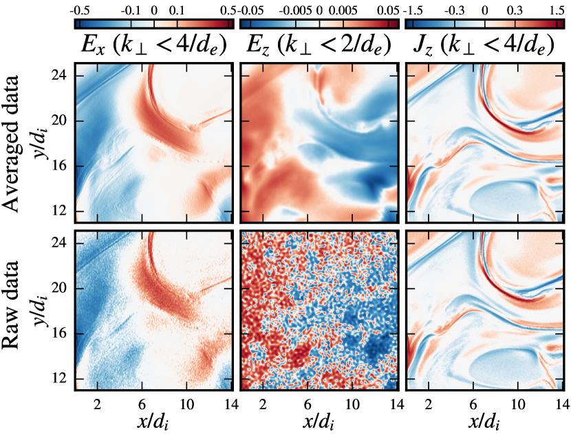
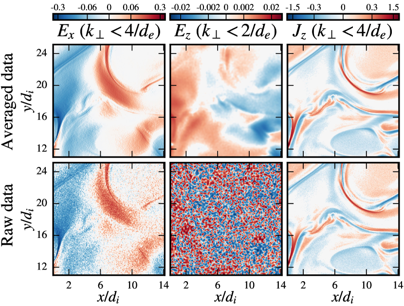
Figure 14: Comparison of the raw and time-averaged PIC data in the $\beta_{i}=0.1$ simulations around 4.7 eddy turnover times for $\epsilon=0.2$ (left) and $\epsilon=0.1$ (right). A doubly-logarithmic scale is used, similar as in Fig. 1. Only a subpart of the entire $x-y$ domain is shown to highlight the small-scale features of the turbulent fields.

In Figure 15 we compare the spectra calculated from the raw and time-averaged data to the estimates for the background particle noise. The turbulent spectra are shown at a single time in the simulation at around 4.7 eddy turnover times. All curves are normalized in such a way that $\sum_{k_{\perp}}P(k_{\perp})$ gives the mean square value of each field in the default physical units adopted in this study (see Sec. 3). The background particle noise is estimated as follows. For each $\beta_{i}$ we initialize a (uniform) thermal plasma with the exact physical parameters as in the turbulence simulations (including a mean magnetic field) but without any (smooth) perturbations that would drive the turbulent cascade. We then integrate the system using the exact same numerical parameters for a few thousand time steps, until the electromagnetic fluctuations driven by discrete particle effects attain a quasi-steady state. We then proceed to calculate the spectra from the thermal plasma simulations and use the results as a proxy for the particle noise in the turbulent runs. As such, our estimate neglects the possible influence of turbulence (in particular, spatial and temporal variations in plasma parameters) on the background noise. However, given the fact that the raw turbulent spectra in Fig. 15 are in relatively good agreement with the PIC noise proxy at the largest wavenumbers, our estimate still appears to be a reasonable one and we are presently unaware of a better alternative for estimating the PIC noise over the entire range of wavenumbers in a turbulent simulation. As shown in Fig. 15, time averaging significantly modifies the turbulent spectra only over the range of wavenumbers, where the raw data is not well-separated from the estimated noise floor (black curves in Fig. 15). Light red/orange shading is used here to indicate the spectral amplitudes that are no more than an order of magnitude below the reference raw data curves. At each given scale, the raw data is decomposed of a mixture of the turbulent signal and particle noise. Therefore, the raw simulation data should be well-separated from the noise floor for the (raw) spectrum to be regarded as physically meaningful at some given scale. The critical wavenumber at which the time-averaged data deviates from the raw data is generally lower for the simulations with a lower value of $\epsilon$ (red/blue curves in Fig. 15). This can be naturally explained by the fact that the relative “signal to noise” ratio is lower in these simulations, because the particle noise does not critically depend on the turbulence amplitude in the first approximation. Similar to a recent work by Haggerty et al. (2017), we find that time averaging modifies the $E_{z}$ spectrum at very large scales. However, as shown in Fig. 15, it is worth considering the fact that the relative strength of particle noise is significantly higher for $E_{z}$ than for any other field. Thus, comparing the turbulent spectra obtained from raw data with those calculated from time-averaged data, without explicitly estimating the strength of particle noise and without visually comparing the data in real space, is not always sufficient to determine whether time averaging is appropriate or not. In summary, we conclude that the time averaging over $\Delta t\approx 0.5\Omega_{ci}^{-1}$ does not seem to significantly modify our simulation results over the range of scales which are well-separated from the noise floor. It does, on the other hand, allow for a more detailed investigation of turbulent structures (in particular for $E_{\perp}$), which are not nearly as clearly recognizable in the raw simulation data.

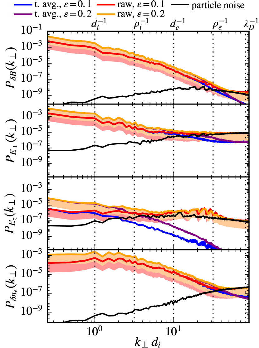
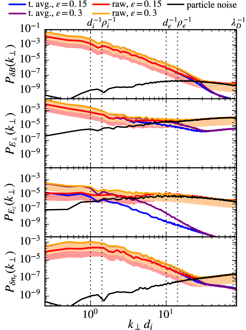
Figure 15: Comparison of the turbulent spectra obtained from raw and time-averaged data to the estimated background particle noise for $\beta_{i}=0.1$ (left) and $\beta_{i}=0.5$ (right). Light red (orange) shading is used to indicate the spectral amplitudes that are no more than an order of magnitude below the reference raw data curves in the low (high) $\epsilon$ simulations. As long as the shading is above the black line, the amplitude of the raw spectrum is more than an order of magnitude above the estimated noise floor.

References

- Alexandrova et al. (2009) Alexandrova, O., Saur, J., Lacombe, C., et al. 2009, PhRvL, 103, 165003
- Bale et al. (2005) Bale, S. D., Kellogg, P. J., Mozer, F. S., Horbury, T. S., & Reme, H. 2005, PhRvL, 94, 215002
- Bañón Navarro et al. (2011) Bañón Navarro, A., Morel, P., Albrecht-Marc, M., et al. 2011, PhRvL, 106, 055001
- Bañón Navarro et al. (2016) Bañón Navarro, A., Teaca, B., Told, D., et al. 2016, PhRvL, 117, 245101
- Birdsall & Langdon (2005) Birdsall, C. K., & Langdon, A. B. 2005, Plasma Physics via Computer Simulation (Taylor & Francis Group, New York)
- Birn et al. (2001) Birn, J., Drake, J. F., Shay, M. A., et al. 2001, JGR, 106, 3715
- Biskamp & Welter (1989) Biskamp, D., & Welter, H. 1989, PhFlB, 1, 1964
- Boldyrev et al. (2013) Boldyrev, S., Horaites, K., Xia, Q., & Perez, J. C. 2013, ApJ, 777, 41
- Boldyrev & Perez (2012) Boldyrev, S., & Perez, J. C. 2012, ApJL, 758, L44
- Brizard & Hahm (2007) Brizard, A. J., & Hahm, T. S. 2007, RvMP, 79, 421
- Bruno & Carbone (2013) Bruno, R., & Carbone, V. 2013, LRSP, 10, 2
- Burch et al. (2016) Burch, J. L., Moore, T. E., Torbert, R. B., & Giles, B. L. 2016, SSRv, 199, 5
- Byers et al. (1978) Byers, J., Cohen, B., Condit, W., & Hanson, J. 1978, JCoPh, 27, 363
- Camporeale & Burgess (2017) Camporeale, E., & Burgess, D. 2017, JPlPh, 83, 535830201
- Cerri & Califano (2017) Cerri, S. S., & Califano, F. 2017, NJPh, 19, 025007
- Cerri et al. (2016) Cerri, S. S., Califano, F., Jenko, F., Told, D., & Rincon, F. 2016, ApJL, 882, L12
- Cerri et al. (2017) Cerri, S. S., Franci, L., Califano, F., Landi, S., & Hellinger, P. 2017, JPlPh, 83, 705830202
- Chang et al. (2014) Chang, O., Gary, S. P., & Wang, J. 2014, PhPl, 21, 052305
- Chasapis et al. (2015) Chasapis, A., Retinò, A., Sahraoui, F., Vaivads, A., & Khotyaintsev, Y. V. 2015, ApJL, 804, L1
- Chen et al. (2013) Chen, C. H. K., Boldyrev, S., Xia, Q., & Perez, J. C. 2013, PhRvL, 110, 225002
- Chen et al. (2014) Chen, C. H. K., Sorriso-Valvo, L., Šafránková, J., & Němeček, Z. 2014, ApJL, 789, L8
- Cho & Lazarian (2009) Cho, J., & Lazarian, A. 2009, ApJ, 701, 236
- Dahlburg & Picone (1989) Dahlburg, R. B., & Picone, J. M. 1989, PhFlB, 1, 2153
- Daughton et al. (2014) Daughton, W., Nakamura, T. K. M., Karimabadi, H., Roytershteyn, V., & Loring, B. 2014, PhPl, 21, 052307
- Dawson (1983) Dawson, J. M. 1983, RvMP, 55, 403
- Fazendeiro & Loureiro (2015) Fazendeiro, L. M., & Loureiro, N. F. 2015, in 42nd EPS Conference on Plasma Physics, ed. R. Bingham, W. Suttrop, S. Atzeni, R. Foest, K. McClements, B. Gonçalves, C. Silva, & R. Coelho, Vol. 39E (Lisbon, Portugal: EPS), P1.402
- Fonseca et al. (2008) Fonseca, R. A., Martins, S. F., Silva, L. O., et al. 2008, PPCF, 50, 124034
- Fonseca et al. (2002) Fonseca, R. A., Silva, L. O., Tsung, F. S., et al. 2002, LNCS, 2331, 342
- Fox et al. (2016) Fox, N. J., Velli, M. C., Bale, S. D., et al. 2016, SSRv, 204, 7
- Franci et al. (2015) Franci, L., Landi, S., Matteini, L., Verdini, A., & Hellinger, P. 2015, ApJ, 812, 21
- Franci et al. (2017) Franci, L., Cerri, S. S., Califano, F., et al. 2017, arXiv:1707.06548
- Frieman & Chen (1982) Frieman, E. A., & Chen, L. 1982, PhFl, 25, 502
- Galtier & Bhattacharjee (2003) Galtier, S., & Bhattacharjee, A. 2003, PhPl, 10, 3065
- Gary & Borovsky (2004) Gary, S. P., & Borovsky, J. E. 2004, JGR, 109, A06105
- Gary et al. (2016) Gary, S. P., Hughes, R. S., & Wang, J. 2016, ApJ, 816, 102
- Gary & Smith (2009) Gary, S. P., & Smith, C. W. 2009, JGR, 114, A12105
- Goldreich & Sridhar (1995) Goldreich, P., & Sridhar, S. 1995, ApJ, 438, 763
- Greco et al. (2012) Greco, A., Valentini, F., & Servidio, S. 2012, PhRvE, 86, 066405
- Haggerty et al. (2017) Haggerty, C. C., Parashar, T. N., Matthaeus, W. H., et al. 2017, arXiv:1706.04905
- Harned (1982) Harned, D. S. 1982, JCoPh, 47, 452
- Hatch et al. (2014) Hatch, D. R., Jenko, F., Bratanov, V., & Bañón Navarro, A. 2014, JPlPh, 80, 531
- Haynes et al. (2014) Haynes, C. T., Burgess, D., & Camporeale, E. 2014, ApJ, 783, 38
- He et al. (2012) He, J., Tu, C., Marsch, E., & Yao, S. 2012, ApJL, 745, L8
- He et al. (2015) He, J., Wang, L., Tu, C., Marsch, E., & Zong, Q. 2015, ApJL, 800, L31
- Henri et al. (2013) Henri, P., Cerri, S. S., Califano, F., et al. 2013, PhPl, 20, 102118
- Hockney (1971) Hockney, R. W. 1971, JCoPh, 8, 19
- Howes (2015) Howes, G. G. 2015, JPlPh, 81, 325810203
- Howes et al. (2006) Howes, G. G., Cowley, S. C., Dorland, W., et al. 2006, ApJ, 651, 590
- Howes et al. (2008a) —. 2008a, JGR, 113, A05103
- Howes et al. (2008b) Howes, G. G., Dorland, W., Cowley, S. C., et al. 2008b, PhRvL, 100, 065004
- Jenko et al. (2000) Jenko, F., Dorland, W., Kotschenreuther, M., & Rogers, B. N. 2000, PhPl, 7, 1904
- Karimabadi et al. (2013) Karimabadi, H., Roytershteyn, V., Wan, M., Matthaeus, W. H., & Daughton, W. 2013, PhPl, 20, 012303
- Kiyani et al. (2009) Kiyani, K. H., Chapman, S. C., Khotyaintsev, Y. V., Dunlop, M. W., & Sahraoui, F. 2009, PhRvL, 103, 075006
- Kiyani et al. (2015) Kiyani, K. H., Osman, K. T., & Chapman, S. 2015, RSPTA, 373, 20140155
- Klein et al. (2017) Klein, K. G., Howes, G. G., & TenBarge, J. M. 2017, JPlPh, 83, 535830401
- Klimontovich (1967) Klimontovich, Y. L. 1967, The Statistical Theory of Non-Equilibrium Processes in a Plasma (Cambridge, Mass.: MIT Press)
- Klimontovich (1997) —. 1997, PhyU, 40, 21
- Kulsrud & Zweibel (2008) Kulsrud, R., & Zweibel, E. G. 2008, RPPh, 71, 046901
- Kunz et al. (2016) Kunz, M. W., Stone, J. M., & Quataert, E. 2016, PhRvL, 117, 235101
- Lacombe et al. (2014) Lacombe, C., Alexandrova, O., Matteini, L., et al. 2014, ApJ, 796, 5
- Lazarian et al. (2015) Lazarian, A., Eyink, G., Vishniac, E., & Kowal, G. 2015, RSPTA, 373, 20140144
- Lazarian & Vishniac (1999) Lazarian, A., & Vishniac, E. T. 1999, ApJ, 517, 700
- Leamon et al. (1998) Leamon, R. J., Smith, C. W., Ness, N. F., & Matthaeus, W. H. 1998, JGR, 103, 4775
- Lele (1992) Lele, S. K. 1992, JCoPh, 103, 16
- Leonardis et al. (2013) Leonardis, E., Chapman, S. C., Daughton, W., Roytershteyn, V., & Karimabadi, H. 2013, PhRvL, 110, 205002
- Leonardis et al. (2016) Leonardis, E., Sorriso-Valvo, L., Valentini, F., et al. 2016, PhPl, 23, 022307
- Li et al. (2016) Li, T. C., Howes, G. G., Klein, K. G., & TenBarge, J. M. 2016, ApJL, 832, L24
- Li & Habbal (2001) Li, X., & Habbal, R. 2001, JGR, 106, 10669
- Liboff (2003) Liboff, R. L. 2003, Kinetic Theory: Classical, Quantum, and Relativistic Descriptions, 3rd edn. (New York: Springer)
- Lifshitz & Pitaevskii (1981) Lifshitz, E. M., & Pitaevskii, L. P. 1981, Physical Kinetics (Oxford: Pergamon Press)
- Liu et al. (2013) Liu, Y.-H., Daughton, W., Karimabadi, H., Li, H., & Roytershteyn, V. 2013, PhRvL, 110, 265004
- Loureiro & Boldyrev (2017) Loureiro, N. F., & Boldyrev, S. 2017, arXiv:1707.05899
- Loureiro et al. (2016) Loureiro, N. F., Dorland, W., Fazendeiro, L., et al. 2016, CoPhC, 206, 45
- Loureiro et al. (2013) Loureiro, N. F., Schekochihin, A. A., & Zocco, A. 2013, PhRvL, 111, 025002
- Loureiro et al. (2009) Loureiro, N. F., Uzdensky, D. A., Schekochihin, A. A., & Cowley, S. C. 2009, MNRAS, 399, L146
- Mallet et al. (2017) Mallet, A., Schekochihin, A. A., & Chandran, B. D. G. 2017, arXiv:1707.05907
- Mangeney et al. (2002) Mangeney, A., Califano, F., Cavazzoni, C., & Travnicek, P. 2002, JCoPh, 179, 495
- Markovskii et al. (2006) Markovskii, S. A., Vasquez, B. J., Smith, C. W., & Hollweg, J. V. 2006, ApJ, 639, 1177
- Marsch (2006) Marsch, E. 2006, LRSP, 3, 1
- Matthaeus & Lamkin (1986) Matthaeus, W. H., & Lamkin, S. L. 1986, PhFl, 29, 2513
- Matthaeus et al. (2016) Matthaeus, W. H., Parashar, T. N., Wan, M., & Wu, P. 2016, ApJL, 827, L7
- Matthaeus et al. (2008) Matthaeus, W. H., Servidio, S., & Dmitruk, P. 2008, PhRvL, 101, 149501
- Matthaeus & Velli (2011) Matthaeus, W. H., & Velli, M. 2011, SSRv, 160, 145
- Matthaeus et al. (2015) Matthaeus, W. H., Wan, M., Servidio, S., et al. 2015, RSPTA, 373, 20140154
- Matthews (1994) Matthews, A. P. 1994, JCoPh, 112, 102
- Muñoz et al. (2017) Muñoz, P. A., Büchner, J., & Kilian, P. 2017, PhPl, 24, 022104
- Muñoz et al. (2015) Muñoz, P. A., Told, D., Kilian, P., Büchner, J., & Jenko, F. 2015, PhPl, 22, 082110
- Narita et al. (2016) Narita, Y., Nakamura, R., Baumjohann, W., et al. 2016, ApJL, 827, L8
- Numata et al. (2010) Numata, R., Howes, G. G., Tatsuno, T., Barnes, M., & Dorland, W. 2010, JCoPh, 229, 9347
- Numata & Loureiro (2015) Numata, R., & Loureiro, N. F. 2015, JPlPh, 81, 305810201
- Okuda & Birdsall (1970) Okuda, H., & Birdsall, C. K. 1970, PhFl, 13, 2123
- Orszag & Tang (1979) Orszag, S. A., & Tang, C.-M. 1979, JFM, 90, 129
- Osman et al. (2011) Osman, K. T., Matthaeus, W. H., Greco, A., & Servidio, S. 2011, ApJL, 727, L11
- Parashar & Matthaeus (2016) Parashar, T., & Matthaeus, W. H. 2016, ApJ, 832, 57
- Parashar et al. (2015a) Parashar, T., Matthaeus, W. H., Shay, M. A., & Wan, M. 2015a, ApJ, 811, 112
- Parashar et al. (2009) Parashar, T., Shay, M., Cassak, P. A., & Matthaeus, W. H. 2009, PhPl, 16, 032310
- Parashar et al. (2015b) Parashar, T. N., Salem, C., Wicks, R. T., et al. 2015b, JPlPh, 81, 905810513
- Passot & Sulem (2015) Passot, T., & Sulem, P. L. 2015, ApJL, 812, L37
- Perrone et al. (2016) Perrone, D., Alexandrova, O., Mangeney, A., et al. 2016, ApJ, 826, 196
- Pezzi et al. (2016) Pezzi, O., Valentini, F., & Veltri, P. 2016, PhRvL, 116, 145001
- Pezzi et al. (2017a) Pezzi, O., Parashar, T. N., Servidio, S., et al. 2017a, ApJ, 834, 166
- Pezzi et al. (2017b) —. 2017b, JPlPh, 83, 705830108
- Picone & Dahlburg (1991) Picone, J. M., & Dahlburg, R. B. 1991, PhFlB, 3, 29
- Podesta (2012) Podesta, J. J. 2012, JGR, 117, A07101
- Podesta et al. (2010) Podesta, J. J., Borovsky, J. E., & Gary, S. P. 2010, ApJ, 712, 685
- Politano et al. (1989) Politano, H., Pouquet, A., & Sulem, P. L. 1989, PhFlB, 1, 2330
- Politano et al. (1995) —. 1995, PhPl, 2, 2931
- Rincon et al. (2016) Rincon, F., Califano, F., Schekochihin, A. A., & Valentini, F. 2016, PNAS, 113, 3950
- Roytershteyn et al. (2015) Roytershteyn, V., Karimabadi, H., & Roberts, A. 2015, RSPTA, 373, 20140151
- Sahraoui et al. (2009) Sahraoui, F., Goldstein, M. L., Robert, P., & Khotyaintsev, Y. V. 2009, PhRvL, 102, 231102
- Saito et al. (2008) Saito, S., Gary, S. P., Li, H., & Narita, Y. 2008, PhPl, 15, 102305
- Salem et al. (2012) Salem, C. S., Howes, G. G., Sundkvist, D., et al. 2012, ApJL, 745, L9
- Schekochihin et al. (2009) Schekochihin, A. A., Cowley, S. C., Dorland, W., et al. 2009, ApJS, 182, 310
- Schekochihin et al. (2016) Schekochihin, A. A., Parker, J. T., Highcock, E. G., et al. 2016, JPlPh, 82, 905820212
- Servidio et al. (2012) Servidio, S., Valentini, F., Califano, F., & Veltri, P. 2012, PhRvL, 108, 045001
- Servidio et al. (2015) Servidio, S., Valentini, F., Perrone, D., et al. 2015, JPlPh, 81, 325810107
- Shaikh & Zank (2009) Shaikh, D., & Zank, G. P. 2009, MNRAS, 400, 1881
- Sundkvist et al. (2007) Sundkvist, D., Retinò, A., Vaivads, A., & Bale, S. D. 2007, PhRvL, 99, 025004
- TenBarge et al. (2014) TenBarge, J. M., Daughton, W., Karimabadi, H., Howes, G. G., & Dorland, W. 2014, PhPl, 21, 020708
- TenBarge & Howes (2012) TenBarge, J. M., & Howes, G. G. 2012, PhPl, 19, 055901
- TenBarge & Howes (2013) —. 2013, ApJL, 771, L27
- Told et al. (2016a) Told, D., Cookmeyer, J., Astfalk, P., & Jenko, F. 2016a, NJPh, 18, 075001
- Told et al. (2016b) Told, D., Cookmeyer, J., Muller, F., Astfalk, P., & Jenko, F. 2016b, NJPh, 18, 065011
- Told et al. (2015) Told, D., Jenko, F., TenBarge, J. M., Howes, G. G., & Hammett, G. W. 2015, PhRvL, 115, 025003
- Tronci & Camporeale (2015) Tronci, C., & Camporeale, E. 2015, PhPl, 22, 020704
- Vaivads et al. (2016) Vaivads, A., Retinò, A., Soucek, J., et al. 2016, JPlPh, 82, 905820501
- Valentini et al. (2014) Valentini, F., Servidio, S., Perrone, D., et al. 2014, PhPl, 21, 082307
- Valentini et al. (2007) Valentini, F., Trávníček, P., Califano, F., Hellinger, P., & Mangeney, A. 2007, JCoPh, 225, 753
- Vasquez et al. (2014) Vasquez, B. J., Markovskii, S. A., & Chandran, B. D. G. 2014, ApJ, 788, 178
- Verscharen et al. (2012) Verscharen, D., Marsch, E., Motschmann, U., & Müller, J. 2012, PhPl, 19, 022305
- Wan et al. (2015) Wan, M., Matthaeus, W. H., Roytershteyn, V., et al. 2015, PhRvL, 114, 175002
- Wan et al. (2016) —. 2016, PhPl, 23, 042307
- Winske et al. (2003) Winske, D., Yin, L., Omidi, N., Karimabadi, H., & Quest, K. 2003, Hybrid Simulation Codes: Past, Present and Future—A Tutorial, ed. J. Büchner, M. Scholer, & C. T. Dum (Berlin, Heidelberg: Springer), 136–165
- Wu et al. (2013a) Wu, P., Wan, M., Matthaeus, W. H., Shay, M. A., & Swisdak, M. 2013a, PhRvL, 111, 121105
- Wu et al. (2013b) Wu, P., Perri, S., Osman, K., et al. 2013b, ApJL, 763, L30
- Zocco & Schekochihin (2011) Zocco, A., & Schekochihin, A. A. 2011, PhPl, 18, 102309