Holographic description of $SO(5)\rightarrow SO(4)$ composite Higgs model

Abstract

We study a 5D bottom-up holographic model that is expected to describe the dynamics of the minimal composite Higgs model characterized by a $SO(5)\to SO(4)$ global symmetry breaking pattern. We assume that the fundamental degrees of freedom are scalars transforming under some representation of $SO(5)$ and subject to some unspecified strong interactions. The holographic description presented here is inspired by previous studies performed in the context of QCD and it allows for the consideration of spin one and spin zero resonances. The resulting spectrum leads in a natural way to a variety of resonances. Namely, those transforming under the unbroken $SO(4)$ subgroup exhibit an exact degeneracy between the two Regge trajectories of vector and scalar channels, while the resonances with quantum numbers in the $SO(5)/SO(4)$ coset lie on a trajectory of (heavier) spin one states and a non-degenerated one of scalar resonances where the four lowest lying ones are massless. These correspond to the four Goldstone bosons in 4D associated to the global symmetry breaking pattern. Restrictions derived from the experimental constraints (Higgs couplings, $S$ parameter, etc.) are then implemented and we conclude that the model is able to accommodate vector and scalar resonances with masses in the range 1 TeV to 2 TeV without encountering phenomenological difficulties. Extension to generic models characterized by the breaking pattern $SO(N)\to SO(N^{\prime}<N)$ is straightforward.

I Introduction

To this date the fundamental nature of the electroweak symmetry breaking sector (EWSBS) of the Standard Model (SM) has not been fully elucidated yet. The majority of the data available so far seems to indicate that the minimal version of the SM with a doublet of complex scalar fields is fully compatible with the data.

However, the jury is still out. There are models where possible departures with respect to the predictions of the SM are small in a natural way. Misaligned composite Higgs models Kaplan and Georgi (1984); *kaplan84-2; *kaplan84-3; *kaplan84-4; *kaplan85 could be considered as a paradigm of this type of theories. In these models a global symmetry group $\mathcal{G}$ is broken down to a subgroup $\mathcal{H}$, that contains the SM global group $SU(2)\times U(1)$. The SM gauge group itself $\mathcal{H}^{\prime}$ is rotated with respect to $\mathcal{H}$ by a certain angle $\theta$ around one of the broken directions. The value of $\theta$ is determined dynamically and it is, roughly speaking, determined by a contribution from the top quark to the Higgs potential (that happens to break the custodial symmetry represented by the global $SU(2)\times SU(2)$ (sub)group of $\mathcal{H}$).

In these models it is a priori possible to establish a large hierarchy between the scale at which the global symmetry breaks (say $4\pi F$), presumably due to some QCD-like new strong interactions, and the weak scale characterized by the Fermi scale $v$, related to the one where in Higgsless models weak interactions may become non-perturbative ($4\pi v$). The latter is customarily regarded as the scale where an extended EWSBS can become strongly interacting. However, a large scale separation, i.e. $F\gg v$ may lead to a relevant amount of fine-tuning in order to keep light the states that should remain in the low energy part of the spectrum.

Having said that, it is a fact that not much is known about the dynamics and the spectrum of theories such as the ones just described. This is particularly true for the models where the global symmetry $\mathcal{G}$ cannot be realized with fermions at the microscopic level, among those is the one introduced first in Agashe et al. (2005) with $\mathcal{G}=SO(5)$ and $\mathcal{H}=SO(4)\simeq SU(2)\times SU(2)$, called the minimal one for providing the most economical way to preserve the custodial symmetry. Yet it is often implicitly assumed that the spectrum in such models can be inferred from what we have learned from QCD, the only relativistic strongly interacting theory that we are familiar with.

It is known that one can get a fairly accurate description of QCD using the so-called bottom-up holographic models, where space-time is extended with an additional dimension $z$, and assumed to be described by an anti-de Sitter (AdS) metric. The value $z=0$ corresponds to the UV brane, where the theory is assumed to be described by a conformal field theory (CFT) as befits a critical point of QCD at short distances. In the IR the holographic model should reproduce the fact that QCD breaks conformality becoming a confining theory. There are two general approaches to this issue. The first one is to introduce an infrared brane, i.e. to restrict the metric of a model to be a slice of the AdS metric; this is the hard wall (HW) proposal Erlich et al. (2005); Da Rold and Pomarol (2005). The second way is to make the AdS metric smoothly cut-off at large $z$; it was put forward in Karch et al. (2006) and referred to as the soft wall (SW) model. Originally inspired by formal developments that establish an exact correspondence between the string theories on $AdS_{5}\times S_{5}$ and $\mathcal{N}=4$ super Yang-Mills gauge theory on $\partial AdS_{5}$ Maldacena (1999); *Gubser1998; *Witten_1998, the bottom-up holographic models are just conjectural. Nevertheless, they provide a surprisingly accurate description of several facets of QCD, such as chiral symmetry breaking in HW and the phenomenological spectra in SW. It is therefore appropriate to try and use these techniques to get precious information on theories whose dynamics is not really known.

The holographic approach has been used before to give a new insight to the known mechanisms of the electroweak symmetry breaking. The minimal composite Higgs scenario was realized first in Agashe et al. (2005); Agashe and Contino (2006) using a HW model, even though the first example of the technique was proposed for the simplest case of the $SU(3)\rightarrow SU(2)$ breaking pattern in Contino et al. (2003). These models have the following characteristics. The gauge symmetry of the SM is extended to the bulk and the symmetry breaking pattern totally relies on the two branes being introduced; the boundary conditions for the 5D fields determine whether they correspond to the dynamical fields or not. The Higgs is associated with the fifth component of gauge fields in the direction of the broken gauge symmetry. The Higgs potential is absent at the tree-level and is determined by quantum corrections (dominantly gauge bosons and top quarks at one-loop level). The extensive study in Agashe et al. (2005); Agashe and Contino (2006) includes a complete calculation of the Higgs potential and analysis of several electroweak observables ($S,\ T,\ Z\rightarrow b\overline{b}$). The stress is made on a way one embeds SM quarks into 5D model (choosing representation etc.) as their contribution is crucial for most of the mentioned computations.

In the present study we use a SW model approach and lay emphasis on an alternative way to realize the global symmetry breaking pattern and to introduce spin zero fields. The $SO(5)\rightarrow SO(4)$ breaking happens in the bulk Lagrangian of the scalar fields, reminiscent to the one of the generalized sigma model used for QCD Gasiorowicz and Geffen (1969); *Fariborz; *Rischke2010. The Goldstone bosons are introduced explicitly and there is no gauge-Higgs unification characteristic to the former studies in the SW framework Falkowski and Perez-Victoria (2008). Gauging of the SM may be achieved via extending the 5D covariant derivative with electroweak bosons, but they are assumed to have no $z$ propagation. They are treated perturbatively on the UV brane and holography is only really relevant to determine the corresponding correlation functions. It is important to emphasize that this approach is quite different from the one adopted in Agashe et al. (2005); Agashe and Contino (2006). In the present proposal the dynamics responsible for the $SO(5)\to SO(4)$ breaking is entirely ‘decoupled’ from the SM gauge fields. The latter are treated in fact as external sources that do not participate in the strong dynamics (except eventually through mixing of fields with identical quantum numbers). We do not consider SM fermion fields either, which in composite Higgs scenarios are essential to provide the Higgs potential Bellazzini et al. (2014); Panico and Wulzer (2016) giving the Higgs mass and self-couplings, among other things. We adopt the point of view that the said potential is of perturbative origin and holographic techniques are not applicable. Needless to say that no new insight into the naturalness problem nor the origin of the hierarchy of the various scales involved is provided. We just attempt to describe the strong dynamics behind the composite sector, the resulting spectrum and verify the fulfilment of the expected current algebra properties, such as the Weinberg sum rules, together with the existing constraints from electroweak precision measurements. In a separate work we will describe the model predictions on coupling constants and form factors of the various resonances resulting from the strong dynamics. Taken together these investigations could shed light on the existence or not of strong dynamics associated to the EWSBS.

Our specific treatment is inspired by various bottom-up holographic approaches to QCD Erlich et al. (2005); Da Rold and Pomarol (2005); Karch et al. (2006); Hirn and Sanz (2005); *Hirn2006; Cappiello et al. (2015) but the spectrum and several properties are quite distinct from them as we will see. We have the necessity to define a fundamental theory (made out of scalar fields in the present case) in order to determine the scalar operators and the conserved currents and to match the normalizations of spin zero and spin one sectors. Other possibilities for the fundamental degrees of freedom are conceivable, but the one presented here is the simplest one.

II General construction

II.1 Strongly interacting sector: operators and misalignment

We will consider extending the SM with an additional strongly interacting sector, assumed to be conformal in the UV. This sector is endowed with a global symmetry that is spontaneously broken. The symmetry breaking pattern is $\mathcal{G}\rightarrow\mathcal{H}$ and the coset $\mathcal{G}/\mathcal{H}$ contains a representation of the Goldstone bosons corresponding to the quantum numbers of the Higgs doublet, and possibly other Goldstone bosons depending on the groups. The coupling to the electroweak sector of the SM is implemented through the conserved currents of the new sector

$$\mathcal{L}=\mathcal{\widetilde{L}}_{str.int.}+\mathcal{L}_{SM}+\widetilde{J}^{a_{L}\ \mu}W_{\mu}^{a_{L}}+\widetilde{J}^{Y\ \mu}B_{\mu}.$$ (1)

The currents of the strongly interacting sector $J^{a_{L}\ \mu}$ and $J^{Y\ \mu}$ contain the generators of the $SU(2)_{L}\times U(1)$ global group that is necessarily included in $\mathcal{H}$. Moreover, these generators belonging to $\mathcal{H}$ are rotated (and marked with tildes) with respect to the SM gauge group $\mathcal{H}^{\prime}$ containing the $W$ and $B$ electroweak gauge bosons. Similarly, we mark with a tilde $\mathcal{L}_{str.int.}$, corresponding to the strongly interacting sector. We will describe this point in more detail below.

Let us now concentrate on the minimal composite Higgs model (MCHM), where the global symmetry breaking pattern is realized as $SO(5)\rightarrow SO(4)$. We denote by $T^{A},\ A=1,...,10$ the generators of $SO(5)$, represented standardly by $5\times 5$ matrices, which are traceless $\operatorname{Tr}T^{A}=0$ and unless otherwise stated have the established normalization $\operatorname{Tr}(T^{A}T^{B})=\delta^{AB}$. They separate naturally into two groups:

• the unbroken generators, in the case of MCHM those of $SO(4)\backsimeq SU(2)_{L}\times SU(2)_{R}$; $T^{a},\ a=1,...,6$ :

  $$T^{\alpha}_{L}=\begin{pmatrix}t^{\alpha}_{L}&0\\ 0&0\\ \end{pmatrix},\ T^{\alpha}_{R}=\begin{pmatrix}t^{\alpha}_{R}&0\\ 0&0\\ \end{pmatrix},\ \alpha=1,2,3,$$ (2)

  where $(t^{\alpha}_{L/R})_{jk}=-\frac{i}{2}(\varepsilon_{\alpha\beta\gamma}\delta^{\beta}_{j}\delta^{\gamma}_{k}\pm(\delta_{j}^{\alpha}\delta_{k}^{4}-\delta_{k}^{\alpha}\delta_{j}^{4}))$, $j,k=1,...,4$.

• the broken generators, corresponding to the coset $SO(5)/SO(4)$; $\widehat{T}^{i},\ i=1,2,3,4$ :

  $$\widehat{T}^{i}_{IJ}=-\frac{i}{\sqrt{2}}(\delta^{i}_{I}\delta^{5}_{J}-\delta^{i}_{J}\delta^{5}_{I}),\ \ I,J=1,...,5.$$ (3)

The MCHM does not admit complex Dirac fermions as fundamental fields at the microscopic level due to the nature of the global symmetry group. Let us assume instead that the theory contains some fundamental scalars transforming under the global $SO(5)$ symmetry. We choose a rank 2 tensor representation, so a fundamental field is a general $5\times 5$ matrix $s^{\alpha\beta}$. The Lagrangian invariant under the global $s\rightarrow gsg^{-1},\ g\in SO(5)$ transformation is $\mathcal{L}=\frac{1}{2}\partial_{\mu}s_{\alpha\beta}\partial^{\mu}s^{\top}_{\beta\alpha}-\frac{1}{2}m^{2}s_{\alpha\beta}s^{\top}_{\beta\alpha}$ . We can construct a scalar invariant $s^{\alpha\gamma}s^{\gamma\alpha}$, giving a scalar operator $\mathcal{O}_{S}^{\alpha\beta}(x)=s^{\alpha\gamma}s^{\gamma\beta}$ with dimension $\Delta=2$, spin $p=0$; and a Noether current $i[T^{A},s]_{\alpha\beta}\partial^{\mu}s^{\top}_{\beta\alpha}$ giving a vector operator $\mathcal{O}_{V}^{A\ \mu}(x)$, with $\Delta=3$, $p=1$. These define the currents of Eqn. (1):

• for $A=a_{L}$: $J^{a_{L}}_{\mu}=\frac{g}{\sqrt{2}}\mathcal{O}^{a_{L}}_{\mu}(x)$;

• for $A=3_{R}$: $J^{Y}_{\mu}=\frac{g^{\prime}}{\sqrt{2}}\mathcal{O}^{3_{R}}_{\mu}(x)$, the hypercharge is assumed to be realized as $Y=T_{3_{R}}$.

The coupling coefficients are chosen to be in concordance with the usual SM normalization of the electroweak generators in the resulting expressions.

Having determined the symmetry breaking pattern in the strongly interacting sector we may come back to the discussion of the vacuum misalignment phenomenon leading to the EWSB. A quantity parametrizing this breaking is a rotation angle $\theta$ that relates the linearly-realized global group $\mathcal{H}=SO(4)$ and a gauged group $\mathcal{H}^{\prime}=SO(4)^{\prime}$ containing the electroweak bosons in its subgroup $SU(2)^{\prime}_{L}\times U(1)^{\prime}$. It is natural to denote the generators of $SO(5)\rightarrow SO(4)^{\prime}$ as $\{T^{a}(0),\ \widehat{T}^{i}(0)\}$ and of $SO(5)\rightarrow SO(4)$ as $\{T^{a}(\theta),\ \widehat{T}^{i}(\theta)\}$ so that $\theta=0$ is assigned to the SM.

We may choose any direction as the one preferred by the $SO(4)^{\prime}$ and then make the misalignment occur with respect to it, this leads to a connection between the generators such as

$$T^{\alpha}(\theta)=r(\theta)T^{\alpha}(0)r^{-1}(\theta),\ \text{with}\ r(\theta)=\begin{pmatrix}1_{3\times 3}&0&0\\ 0&\cos(\theta)&\sin(\theta)\\ 0&-\sin(\theta)&\cos(\theta)\\ \end{pmatrix}.$$ (4)

This only affects the relation between the SM gauge generators and those of the strongly interacting sector, hence the tildes in Eqn. (1). A 5D dual model we proceed to define in the next subsection is not influenced by the misalignment effect. It is an alternative way to describe the physics involved in the $SO(5)\rightarrow SO(4)$ symmetry breaking, derived from some interactions becoming strong in the infrared.

II.2 5D model Lagrangian

In this subsection we describe the holographic 5D model realizing some conceptual features of the 4D MCHM. See, for instance, the review Panico and Wulzer (2016) presenting various aspects of 4D studies, though we do not address at all the flavour issues discussed in abundance in the literature.

We have selected two composite operators – a vector and a scalar one, to be defining to the theory, and hence we have spin one and spin zero fields at the 5D side. The choice is motivated by the AdS/QCD models where a quark bilinear and left- and right-handed currents corresponding to the chiral flavour symmetry are supposed to be important for the description of the chiral dynamics.

The 5D AdS metric (with the radius $R$) is given by

$$g_{MN}dx^{M}dx^{N}=\frac{R^{2}}{z^{2}}(\eta_{\mu\nu}dx^{\mu}dx^{\nu}-d^{2}z),\quad\eta_{\mu\nu}=\text{diag}(1,-1,-1,-1).$$ (5)

The $SO(5)$ invariant action that we assume has the following form

$$S_{5D}=-\frac{1}{4g_{5}^{2}}\int d^{5}x\sqrt{-g}e^{-\Phi(z)}\operatorname{Tr}F_{MN}F_{KL}g^{MK}g^{LN}+$$ (6)

$$+\frac{1}{k_{s}}\int d^{5}x\sqrt{-g}e^{-\Phi(z)}\bigg{[}\operatorname{Tr}g^{MN}(D_{M}H)^{\top}(D_{N}H)-M^{2}\operatorname{Tr}HH^{\top}-M^{2}\operatorname{Tr}(HD^{\top}+H^{\top}D)\bigg{]}$$

As was previously mentioned this 5D effective action draws its inspiration from generalized sigma models including spin zero and spin one fields that have been used in the context of strong interactions. The normalization constants have the dimensionality $[g_{5}^{2}]=[k_{s}]=L^{1}$ to compensate that of the additional dimension. Following the SW holographic approach we have introduced a dilaton $\Phi(z)$. Together with the metric $g_{MN}$ it gives the gravitational background of a smoothly capped off spacetime.

The field strength tensor is

$$F_{MN}=(\partial_{M}A_{N}^{A}-\partial_{N}A_{M}^{A}+C^{ABC}A^{B}_{M}A^{C}_{N})T^{A},$$ (7)

where the upper index runs through both broken and unbroken indices $A_{M}=A_{M}^{A}T^{A}=A_{M}^{a}T^{a}+A_{M}^{i}\widehat{T}^{i}$. This vector field is unrelated to the $W$ or $B$ gauge bosons of the electroweak interactions. It is dual to the vector composite operator $i\operatorname{Tr}[T^{A},s]\partial^{\mu}s^{\top}$. $H$ is dual to the scalar composite operator $ss$. It is a matrix valued scalar field that contains the Goldstone bosons associated to the breaking of the global symmetry as well as other scalar fields describing perturbations in the unbroken directions. The last term of Eqn. (6) appears as a shifted vacuum expectation value $H\rightarrow H+D$ and will play a crucial role in getting the phenomenological spectrum.

The dynamical breaking from $SO(5)$ to $SO(4)$ is present due to a function $f(z)$ appearing in the nonlinear parametrization of the field $H$:

$$H=\xi\Sigma\xi^{-1},\quad\Sigma=\begin{pmatrix}0_{4\times 4}&0\\ 0&f(z)\\ \end{pmatrix}+iT^{a}\sigma^{a}(x,z),\quad\xi=\exp\left(\frac{i\Pi^{i}(x,z)\widehat{T}^{i}}{\sqrt{2}f(z)}\right)$$ (8)

If the group elements are denoted $g\in SO(5)$ and $h\in SO(4)$, the fields transform as

$$\xi\rightarrow\xi^{\prime}=g\xi h^{-1},\ \Sigma\rightarrow\Sigma^{\prime}=h\Sigma h^{-1},\ H\rightarrow H^{\prime}=gHg^{-1}.$$ (9)

The action would be fully $SO(5)$ invariant if the matrix D transformed under $SO(5)$ as $D\to gDg^{-1}$. However, we adopt the following form for $D$:

$$D=\begin{pmatrix}0_{4\times 4}&0\\ 0&b(z)\\ \end{pmatrix},$$ (10)

therefore making the last term of Eqn. (6) only $SO(4)$ invariant. The function $b(z)$ parametrizes a soft breaking of $SO(5)$ down to $SO(4)$ in the 5D holographic model.

Holography prescribes that every global symmetry of the 4D model comes as a gauge symmetry of its 5D dual. Thus, to make the Lagrangian invariant under the gauge transformation $A_{M}\rightarrow A^{\prime}_{M}=gA_{M}g^{-1}+ig\partial_{M}g^{-1}$ the covariant derivative is introduced in the 5D action (6), defined as

$$D_{M}H=\partial_{M}H-i[A_{M},H],\quad D_{M}H\rightarrow gD_{M}Hg^{-1}.$$ (11)

We choose to work within $A_{z}=0$ gauge , in which the scalar kinetic term simplifies to

$$g^{MN}(D_{M}H)^{\top}(D_{N}H)=g^{\mu\nu}(D_{\mu}H)^{\top}(D_{\nu}H)-\frac{z^{2}}{R^{2}}(\partial_{z}H)^{\top}(\partial_{z}H).$$ (12)

Expanding the scalar matrix $H$ we rewrite the action (6) in terms of 6 scalar ($\sigma^{a}$), 4 Goldstone ($\Pi^{i}$) and 10 vector ($A_{\mu}^{a/i}$) composite fields:

$$S_{5D}= \int d^{5}x\sqrt{-g}e^{-\Phi(z)}\left(-\frac{1}{4g_{5}^{2}}\operatorname{Tr}\left(F_{\mu\nu}F_{\lambda\rho}g^{\mu\lambda}g^{\nu\rho}-\frac{z^{2}}{R^{2}}g^{\mu\nu}\partial_{z}A_{\mu}\partial_{z}A_{\nu}\right)+\frac{1}{k_{s}}g^{\mu\nu}f^{2}(z)A^{i}_{\mu}A^{i}_{\nu}\right)+$$

$$+\frac{1}{k_{s}}\int d^{5}x\sqrt{-g}e^{-\Phi(z)}\Bigg{[}g^{\mu\nu}\partial_{\mu}\sigma^{a}\partial_{\nu}\sigma^{a}-\frac{z^{2}}{R^{2}}\partial_{z}\sigma^{a}\partial_{z}\sigma^{a}-M^{2}\sigma^{a}\sigma^{a}+$$ (13)

$$+\frac{1}{2}g^{\mu\nu}\partial_{\mu}\Pi^{i}\partial_{\nu}\Pi^{i}-\frac{1}{2}\frac{z^{2}}{R^{2}}\partial_{z}\Pi^{i}\partial_{z}\Pi^{i}-M^{2}f(z)b(z)\cos{\frac{\sqrt{\Pi^{i}\Pi^{i}}}{f(z)}}-\sqrt{2}f(z)g^{\mu\nu}A^{i}_{\mu}\partial_{\nu}\Pi^{i}\Bigg{]}.$$

After imposing the $A_{z}=0$ gauge we still have enough gauge freedom left to set $\partial^{\mu}A^{i}_{\mu}=0$ and the mixing of the scalar $\Pi^{i}$ and the longitudinal part of $A^{i}_{\mu}$ can be neglected.

The ansätze for the background functions $\Phi(z)$, $f(z)$ and $b(z)$ will be proposed below.

II.3 AdS/CFT prescriptions

Let us discuss briefly what basic holographic assumptions and prescriptions should be taken into account.

The new strongly interacting sector being confining is supposed to have some non-Abelian gauge group, which could be characterized with the number of ‘technicolours’ $N_{tc}$. In AdS/CFT the duality is valid only in the large-$N_{tc}$ limit; however, we will relax this condition when applying it to phenomenology.

All bulk fields are prescribed to acquire a mass following the general formula $M^{2}R^{2}=(\Delta-p)(\Delta+p-4)$, where $\Delta$ and $p$ are respectively a dimension and a spin of a dual operator Gubser et al. (1998); *Witten_1998. Hence, the gauge fields $A^{A}_{\mu}(x,z)$ have $M^{2}R^{2}=0$ and the scalar field $H(x,z)$ gets $M^{2}R^{2}=-4$, the last is in fact the lowest value allowed by the Breitenlohner-Freedman bound.

From the 5D model given by Eqn. (6) one can extract the n-point correlation functions of the composite operators. The 4D partition function in the discussed model is given analogously to any quantum field theory by

$$\mathcal{Z}_{4D}[\phi_{\mathcal{O}}] = \int[\mathcal{D}s]\operatorname{Exp}i\int d^{4}x[\mathcal{L}_{str.int.}(x)+\phi_{\mathcal{O}\mu}^{A}(x)\operatorname{Tr}\partial^{\mu}s[iT^{A},s](x)+\phi_{\mathcal{O}}^{\alpha\beta}(x)s_{\beta\gamma}s_{\gamma\alpha}(x)]=$$ (14)

$$= \operatorname{Exp}\sum\limits_{q}\frac{1}{q!}\int\prod\limits_{k=1}^{q}d^{4}x_{k}\langle\mathcal{O}_{1}(x_{1})...\mathcal{O}_{q}(x_{q})\rangle i\phi_{\mathcal{O}}^{1}(x_{1})...i\phi_{\mathcal{O}}^{q}(x_{q}),$$

where $\phi_{\mathcal{O}\mu}^{A}(x)$ and $\phi_{\mathcal{O}}^{\alpha\beta}(x)$ are the sources of the composite operators. The AdS/CFT correspondence principle states the equivalence between the partition function in the 4D theory and the 5D holographic effective acion when the last one is on-shell:

$$\mathcal{Z}_{4D}[\phi_{\mathcal{O}}]=\operatorname{Exp}iS_{5D}^{on-shell}|_{\phi(x,z)\rightarrow\phi(x,z=\varepsilon)}.$$ (15)

Going on-shell is accompanied with setting all 5D bulk fields $\phi(x,z)$ to their boundary values at $z=\varepsilon$ ($\varepsilon$ being an UV regulator), which basically coincide with the sources $\phi_{\mathcal{O}}$. We should be more careful at this point, however. For the gauge fields the matching is simple $A^{A}_{\mu}(x,z)|_{z=\varepsilon}=\phi_{\mathcal{O}\mu}^{A}(x)$, while a general scalar matrix valued field $H$ is connected to the source via $H^{\alpha\beta}(x,z)|_{z=\varepsilon}=R^{-1}\varepsilon^{d-\Delta}\phi_{\mathcal{O}}^{\alpha\beta}(x)$, where an additional length scale is introduced to have $[H]=E^{1},\ [\phi_{\mathcal{O}}]=E^{d-\Delta}$. For the degenerate situation when $\sqrt{\frac{d^{2}}{4}+M^{2}R^{2}}=0$, which is the case for $d=4,\ \Delta=2$, the connection contains a logarithm as well: $H^{\alpha\beta}(x,z)|_{z=\varepsilon}=R^{-1}\varepsilon^{2}\ln\left(\frac{\varepsilon}{R}\right)^{2}\phi_{\mathcal{O}}^{\alpha\beta}(x)$ Klebanov and Witten (1999); Minces and Rivelles (2000). The Green’s functions can therefore be obtained by differentiating the 5D effective action with respect to the sources.

Now we would like to prescribe the sources to real physical degrees of freedom, meaning the fields $\sigma$ and $\Pi$. It is clear that quantum fluctuations of $H$ can be splitted into symmetric and antisymmetric parts $H(x,z)|_{z=\varepsilon}=T_{sym}^{i}H_{sym}^{i}(x,\varepsilon)+T_{asym}^{a}H_{asym}^{a}(x,\varepsilon)$. Though they do not span the ${\bf 10}_{A}$ and ${\bf 14}_{S}$ representation spaces of $SO(5)$ (as $H$ itself does not span the whole space of $5\times 5$ matrices), they can be written in terms of generators forming the basis for ${\bf 10}_{A}$ and ${\bf 14}_{S}$. Taking into account the nonlinear realization of $H$ one has an argument of the large-$N_{tc}$ limit for linearizing the boundary value of $H$ as follows: $H(x,z)|_{z=\varepsilon}\simeq iT^{a}\sigma^{a}(x,\varepsilon)+\widehat{T}_{sym}^{i}\Pi^{i}(x,\varepsilon)/\sqrt{2},$ where $T^{a}$ of Eqn. (2) form a subset in the basis of ${\bf 10}_{A}$ and $\widehat{T}_{sym}^{i}$ – in the basis of ${\bf 14}_{S}$, and are defined as $\widehat{T}_{sym\ \alpha\beta}^{i}=\frac{1}{\sqrt{2}}(\delta^{i}_{\alpha}\delta_{\beta}^{5}+\delta_{\beta}^{i}\delta_{\alpha}^{5})$. One may perform a similar expansion in the sources $\phi_{\mathcal{O}\ \alpha\beta}=s^{a}_{\mathcal{O}}\cdot iT^{a}_{\alpha\beta}+p^{i}_{\mathcal{O}}\cdot\widehat{T}^{i}_{sym\ \alpha\beta}$. Then it is straightforward to establish the connections between the new sources and composite operators related to the unbroken/broken directions:

$$s^{a}_{\mathcal{O}}(x)=R\varepsilon^{-2}\ln^{-1}\left(\frac{\varepsilon}{R}\right)^{2}\times\sigma^{a}(x,\varepsilon),\ \text{dual to}\ \mathcal{O}_{s}^{a}=iT^{a}_{\alpha\beta}s_{\beta\gamma}s_{\gamma\alpha}(x);$$ (16)

$$p^{i}_{\mathcal{O}}(x)=R\varepsilon^{-2}\ln^{-1}\left(\frac{\varepsilon}{R}\right)^{2}\times\frac{\Pi^{i}(x,\varepsilon)}{\sqrt{2}},\ \text{dual to}\ \mathcal{O}_{p}^{i}=\widehat{T}^{i}_{sym\ \alpha\beta}s_{\beta\gamma}s_{\gamma\alpha}(x).$$ (17)

A general 5D field is a solution of a second order equation of motion (EOM) and has two modes. The leading at small $z$ mode gives a connection between a source at the boundary and a value of a field in the bulk through the bulk-to-boundary propagator. This mode should also exhibit enough decreasing behaviour at $z\rightarrow+\infty$ to render the on-shell action finite. The subleading mode provides a set of normalizable solutions, which could be identified with a tower of physical states at the 4D boundary. This is the standard Kaluza-Klein (KK) mode: the 5D field is presented as an infinite series of 4D fields weighted with the $z$-dependent profile functions. A boundary condition should be chosen for this profile and we prefer the Dirichlet one through all the paper.

It is important to understand that the 5D fields do not represent ‘particles’. Therefore it should not come as a surprise the following situation that is one of the focal points of our work: if one sets the $SO(5)$ - breaking term $b(z)$ equal to zero, there is no quadratic term in the 5D action Eqn. (13) for the $\Pi^{i}$. However, this does not mean that the particles forming the KK tower are massless. In fact they are not. The role of the symmetry breaking term will be to shift those masses so that the lowest lying state can be identified as a genuine Goldstone boson.

In the following sections we show how this AdS/CFT dictionary works in practice in the model under consideration.

III Unbroken generators

III.1 Vector fields

For the vector fields corresponding to the unbroken generators with $a=1,...,6$, taking only transverse part, we get the equation of motion from the action (13)

$$\left(\partial_{z}\frac{e^{-\Phi}}{z}\partial_{z}A^{a}_{\mu}-\frac{e^{-\Phi}}{z}\Box A_{\mu}^{a}\right)_{\bot}=0.$$ (18)

The dilaton background is assumed to have the standard quadratic form $\Phi(z)=\kappa^{2}z^{2}$ Karch et al. (2006) throughout the paper. We perform a 4D Fourier transform $A_{\mu}^{a}(x,z)=\int d^{4}qe^{iqx}A_{\mu}^{a}(q,z)$ and focus on finding first the bulk-to-boundary propagator, which we call $V(q,z)$. Following the holographic prescriptions, we know that

$$A_{\mu}^{a}(q,z)=V(q,z)\phi_{\mathcal{O}\mu}^{a}(q),\quad\ V(q,\varepsilon)=1$$ (19)

Then, after a suitable change of variables $y=\kappa^{2}z^{2}$ we arrive at the following EOM:

$$yV^{\prime\prime}(q,y)-yV^{\prime}(q,y)+\frac{q^{2}}{4\kappa^{2}}V(q,y)=0$$ (20)

It is a particular case of the confluent hypergeometric equation (see Appendix A for a review of the properties and solutions of this equation), and the solution is

$$V(q,\kappa^{2}z^{2})=C(q)\kappa^{2}z^{2}\ _{1}F_{1}\left(-\frac{q^{2}}{4\kappa^{2}}+1,2;\kappa^{2}z^{2}\right)+\Gamma\left(-\frac{q^{2}}{4\kappa^{2}}+1\right)\Psi\left(-\frac{q^{2}}{4\kappa^{2}},0;\kappa^{2}z^{2}\right),$$ (21)

where $\Psi$ is the Tricomi’s function. The second term is dominant at small $z$ and represents the propagator.

The first term gives us the tower of massive states, which could be identified with some physical states at the boundary. Normalizable solutions can only be found for discrete values of the 4D momentum $q^{2}=M_{V}^{2}(n)$ and we may identify $\left.V(q,z)\right|_{q^{2}=M_{V}^{2}(n)}=V_{n}(z)$. Then, the KK decomposition is given as

$$A^{a}_{\mu}(q,z)=\sum\limits_{n=0}^{\infty}V_{n}(z)A_{\mu(n)}^{a}(q).$$ (22)

The $z$ profile is determined from (21) and the spectrum can be expressed using the discrete parameter $n=0,1,2,...$:

$$V_{n}(z)=\kappa^{2}z^{2}\sqrt{\frac{2}{n+1}}L_{n}^{1}(\kappa^{2}z^{2}),\quad\ M_{V}^{2}(n)=4\kappa^{2}(n+1),$$ (23)

where $L_{n}^{m}(x)$ are the generalised Laguerre polynomials. The $V_{n}(z)$ are subject to the Dirichlet boundary condition and are normalized to fulfil the orthogonality relation:

$$\int\limits_{0}^{\infty}dze^{-\kappa^{2}z^{2}}z^{-1}V_{n}(z)V_{k}(z)=\delta_{nk},$$ (24)

the weight there is dictated by the form of the initial operator in Eqn. (18).

III.2 Scalar fields

The EOM for the $\sigma(x,z)$ fields obtained from the action (13) is:

$$\partial_{z}\frac{e^{-\Phi}}{z^{3}}\partial_{z}\sigma^{a}-\frac{e^{-\Phi}}{z^{3}}\Box\sigma^{a}-\frac{M^{2}R^{2}}{z^{5}}e^{-\Phi}\sigma^{a}=0.$$ (25)

As before we take $\Phi(z)=\kappa^{2}z^{2}$. Making a 4D Fourier transformation and the substitution $\sigma^{a}(q,z)=(\kappa^{2}z^{2})^{1-\sqrt{1+M^{2}R^{2}/4}}\widetilde{\sigma^{a}}(\kappa^{2}z^{2},q)$ we arrive at a confluent hypergeometric equation for $\widetilde{\sigma}^{a}(z,q)$, which is conveniently written in terms of $y=\kappa^{2}z^{2}$ as

$$y\widetilde{\sigma}^{\prime\prime}_{a}(q,y)+\left(1-\sqrt{4+M^{2}R^{2}}-y\right)\widetilde{\sigma}^{\prime}_{a}(q,y)-\left(1-\frac{q^{2}}{4\kappa^{2}}-\sqrt{1+\frac{M^{2}R^{2}}{4}}\right)\widetilde{\sigma}_{a}(q,y)=0.$$ (26)

For the case $M^{2}R^{2}=-4$ it has the following solutions expressed in terms of the $z$ variable

$$\sigma^{a}(q,z)=C_{1}(q)(\kappa^{2}z^{2})\ _{1}F_{1}\left(1-\frac{q^{2}}{4\kappa^{2}},1;\kappa^{2}z^{2}\right)+C_{2}(q)(\kappa^{2}z^{2})\Psi\left(1-\frac{q^{2}}{4\kappa^{2}},1;\kappa^{2}z^{2}\right).$$ (27)

Now, we have two modes with the seemingly same small $z$ behaviour. This is expected in the AdS/CFT setting for $\Delta=2$ scalar operators Klebanov and Witten (1999); Minces and Rivelles (2000). However, it is known that the Tricomi’s function ($\Psi$) with an integer second parameter exhibits a logarithmic behaviour (see Eqn. (110)). This proves it to be the mode representing the bulk-to-boundary propagator.

To find the normalizable solutions we solve the eigenvalue problem imposing $q^{2}=M_{\sigma}^{2}(n)$ and demanding the Dirichlet boundary condition to be fulfilled for the eigenmodes. We express this solution in terms of the Laguerre polynomials as:

$$\sigma^{a}(q,z)=\sum\limits_{n=0}^{\infty}R^{-1}\sigma_{n}(z)\sigma^{a}_{(n)}(q),\quad\sigma_{n}(z)=N(\kappa z)^{2}L_{n}(\kappa^{2}z^{2}),$$ (28)

where $n=\frac{M_{\sigma}^{2}(n)}{4\kappa^{2}}-1$. The normalization is $N^{2}=\frac{2}{\kappa^{2}}$ and $\int\limits_{0}^{\infty}dze^{-\kappa^{2}z^{2}}z^{-3}\sigma_{n}(z)\sigma_{k}(z)=\delta_{nk}$. Note that the $z$-profiles $\sigma_{n}(z)$ have the dimensionality $E^{-1}$, which is correct, as the dimensionality of the Green’s function corresponding to the operator of Eqn. (25) is $E^{-4}$. Hence, we include the dimensionful $R$ in the KK decomposition. Compare with the discussion about the scalar sources, where an additional $R$ also appears.

The mass spectrum is

$$M_{\sigma}^{2}(n)=4\kappa^{2}(n+1+\sqrt{1+M^{2}R^{2}/4})=4\kappa^{2}(n+1),\ n=0,1,2...$$ (29)

The proposed treatment of the scalar fields is parallel to the AdS/QCD one Colangelo et al. (2008) (for a HW alternative see Da Rold and Pomarol (2006)) but for the fact of having another $\Delta$ and $M^{2}R^{2}=-4$. Unlike QCD in general and its AdS/QCD imitation, we observe a degeneracy between the scalar and the vector fields associated to the unbroken generators.

IV Broken generators

IV.1 Vector fields

For the transverse part of the fields corresponding to the broken generators with $i=1,2,3,4$ we get the EOM:

$$\left(\partial_{z}\frac{e^{-\Phi}}{z}\partial_{z}A_{\mu}^{i}-\frac{e^{-\Phi}}{z}\Box A_{\mu}^{i}-2\frac{g_{5}^{2}f^{2}(z)}{k_{s}}e^{-\Phi}\frac{R^{2}}{z^{3}}A_{\mu}^{i}\right)_{\bot}=0.$$ (30)

As in the unbroken case we perform the 4D Fourier transformation and establish the propagation between the source and the bulk:

$$A_{\mu}^{i}(q,z)=A(q,z)\phi_{\mathcal{O}\mu}^{i}(q),\qquad A(q,\varepsilon)=1.$$ (31)

Changing variables to $y=\kappa^{2}z^{2}$ again we arrive at the following EOM

$$yA^{\prime\prime}(q,y)-yA^{\prime}(q,y)+\left(\frac{q^{2}}{4\kappa^{2}}-\frac{(g_{5}Rf(y))^{2}}{2yk_{s}}\right)A(q,y)=0.$$ (32)

Now we need to choose the $z$ dependence for $f(z)$. In order to get an analytical solution we have to assume that either $f^{2}(y)\sim y$ or $f^{2}(y)\sim$ constant. The last option taken together with the boundary condition on $A(q,z)$ demands the implausible relation $f(y)=0$. Then, consider the linear ansatz $f(z)=f\cdot\kappa z$, where the constant $f$ has the dimension of mass. The solution of the confluent hypergeometric equation above is

$$A(q,\kappa^{2}z^{2}) = C(q)\kappa^{2}z^{2}\ _{1}F_{1}\left(-\frac{q^{2}}{4\kappa^{2}}+\frac{(g_{5}Rf)^{2}}{2k_{s}}+1,2;\kappa^{2}z^{2}\right)+$$

$$+\Gamma\left(-\frac{q^{2}}{4\kappa^{2}}+\frac{(g_{5}Rf)^{2}}{2k_{s}}+1\right)\Psi\left(-\frac{q^{2}}{4\kappa^{2}}+\frac{(g_{5}Rf)^{2}}{2k_{s}},0;\kappa^{2}z^{2}\right).$$

The second term defines the propagator, while the first for discrete values of $q^{2}$ and $\left.A(q,z)\right|_{q^{2}=M_{A}^{2}(n)}=A_{n}(z)$ gives the $z$-profiles and masses of the eigenstates

$$A_{n}(z)=\kappa^{2}z^{2}\sqrt{\frac{2}{n+1}}L_{n}^{1}(\kappa^{2}z^{2}),\quad M_{A}^{2}(n)=4\kappa^{2}\left(n+1+\frac{(g_{5}Rf)^{2}}{2k_{s}}\right),\quad n=0,1,2....$$ (34)

We observe that the pattern of the Regge trajectory is similar to the one found for the vector states corresponding to the unbroken generators, but the intercept is larger. That means that these states are heavier than their unbroken counterparts. We postpone to a latter section a tentative phenomenological discussion.

IV.2 Goldstone bosons

The part of the action (13) describing the $\Pi^{i}(x,z),\ i=1,2,3,4$ fields leads to the EOM

$$\partial_{z}\frac{e^{-\Phi}}{z^{3}}\partial_{z}\Pi^{i}-\frac{e^{-\Phi}}{z^{3}}\Box\Pi^{i}+\frac{R^{2}}{z^{5}}\frac{b(z)}{f(z)}M^{2}e^{-\Phi}\Pi^{i}=0.$$ (35)

We define $B(z)=\frac{b(z)}{f(z)}$ in substitution of the unknown $b(z)$. Changing variables to $y=\kappa^{2}z^{2}$ we arrive at the following EOM

$$y{\Pi_{i}}^{\prime\prime}(q,y)+(-1-y){\Pi_{i}}^{\prime}(q,y)+\left(\frac{q^{2}}{4\kappa^{2}}+\frac{R^{2}}{4y}M^{2}B(y)\right)\Pi_{i}(q,y)=0.$$ (36)

We choose a polynomial ansatz for $B(y)=\mu_{1}+\mu_{2}y$. Addition of higher order terms would bring us to the so-called extended confluent hypergeometric equation, solutions of which are not easily tractable.

Consider the change of variables $\Pi_{i}(q,y)=y^{\beta}\widetilde{\Pi_{i}}(q,y)$, where $\beta_{\pm}=1\pm\sqrt{1-\frac{M^{2}R^{2}}{4}\mu_{1}}=1\pm\frac{1}{2}m$ is chosen to cancel the $y^{-1}$ terms in Eqn. (36). Then the EOM reads

$$y\widetilde{\Pi}_{i}^{\prime\prime}(q,y)+(1\pm m-y)\widetilde{\Pi}_{i}^{\prime}(q,y)+\left(\frac{q^{2}}{4\kappa^{2}}+\frac{M^{2}R^{2}}{4}\mu_{2}-(1\pm\frac{1}{2}m)\right)\widetilde{\Pi}_{i}(q,y)=0.$$ (37)

Due to the properties of the confluent hypergeometric functions, the $\beta_{+}$ and $\beta_{-}$ cases are virtually the same; i.e. transforming one into another at different values of parameters (see Eqn. (111) in Appendix A). As we expect $m$ to be a positive integer number, we choose the solution:

$$\Pi^{i}(q,\kappa^{2}z^{2}) =C_{1}(q)(\kappa^{2}z^{2})^{1+\frac{1}{2}m}\ _{1}F_{1}\left(1+\frac{1}{2}m-\frac{q^{2}}{4\kappa^{2}}-\frac{M^{2}R^{2}}{4}\mu_{2},1+m;\kappa^{2}z^{2}\right)+$$

$$+C_{2}(q)(\kappa^{2}z^{2})^{1+\frac{1}{2}m}\Psi\left(1+\frac{1}{2}m-\frac{q^{2}}{4\kappa^{2}}-\frac{M^{2}R^{2}}{4}\mu_{2},1+m;\kappa^{2}z^{2}\right).$$ (38)

Looking for a normalizable solution for discrete values $q^{2}=M_{\Pi}^{2}(n)$ we arrive at the KK decomposition with the specific 5D profiles

$$\Pi^{i}(q,z)=\sum\limits_{n=0}^{\infty}R^{-1}\Pi_{n}(z)\Pi^{i}_{(n)}(q),\quad\Pi_{n}(z)=N(\kappa z)^{2+m}L_{n}^{m}(\kappa^{2}z^{2}),$$ (39)

where $n=-1-\frac{1}{2}m+\frac{M_{\Pi}^{2}(n)}{4\kappa^{2}}+\frac{M^{2}R^{2}}{4}\mu_{2},\ m=\sqrt{4-M^{2}R^{2}\mu_{1}}$. The normalization is analogous to that of $\sigma(x,z)$ fields: $N^{2}=\frac{2}{\kappa^{2}}$ and $\int\limits_{0}^{\infty}dze^{-\kappa^{2}z^{2}}z^{-3}\Pi_{n}(z)\Pi_{k}(z)=\delta_{nk}$.

Thus, we obtain the following mass spectrum depending on the parameters $m$ (or $\mu_{1}$) and $\mu_{2}$ of the ansatz:

$$M_{\Pi}^{2}(n)=4\kappa^{2}\left(n+1+\frac{1}{2}m-\frac{M^{2}R^{2}}{4}\mu_{2}\right).$$ (40)

Having found the general solution, we focus on the case of $M^{2}R^{2}=-4$ and fix the values of $\mu_{1}$ and $\mu_{2}$. To determine $\mu_{1}$ let us turn to the bulk-to-boundary propagator connecting the 5D bulk value to the source; its boundary behaviour is fixed by the AdS/CFT prescription:

$$\Pi^{i}(q,\kappa^{2}z^{2})=\Pi^{prop}(q^{2}/\kappa^{2},\kappa^{2}z^{2})p^{i}_{\mathcal{O}}(q)\ \xrightarrow{z\rightarrow\varepsilon}\ \Pi^{i}(q,\kappa^{2}\varepsilon^{2})=\sqrt{2}\varepsilon^{2}R^{-1}\ln\left(\frac{\varepsilon}{R}\right)^{2}p^{i}_{\mathcal{O}}(q).$$ (41)

Taking into account that $\Pi^{prop}(q^{2}/\kappa^{2},\kappa^{2}z^{2})$ must be well-behaved at $z\rightarrow+\infty$, we conclude that only the $\Psi$-function term in Eqn. (38) with $m=0$ (equivalent to $\mu_{1}=-1$) can provide the correct solution. As now we have the value of $m$ fixed, the eigenmodes have the $z$-profiles and the spectrum

$$\Pi_{n}(z)=\sqrt{\frac{2}{\kappa^{2}}}(\kappa z)^{2}L_{n}(\kappa^{2}z^{2}),\quad M_{\Pi}^{2}(n)=4\kappa^{2}\left(n+1+\mu_{2}\right),\quad n=0,1,2...$$ (42)

By choosing $\mu_{2}=-1$ we obtain the result that for $n=0$, $M_{\Pi}^{2}(0)=0$. This is remarkable as it provides us with a multiplet of massless Goldstone bosons, a result that is not easy to get in the holographic approach or in the Regge theory. If we look at the origin of this more closely we see that it is due to the combination of the two terms contributing to the mass in Eqn. (6). Note that the term linear in $H$ only contributes to the symmetric part of this matrix valued field ($H$ is not in an irrep of $SO(5)$).

V Correlation functions

In this section we summarize the two-point correlation functions derived in the four channels just discussed.

V.1 Unbroken generators

Following the holographic prescriptions given by Eqns. (14) and (15) we define the vector correlation function as

$$\langle\mathcal{O}_{\mu}^{a}(q)\mathcal{O}_{\nu}^{b}(p)\rangle=\delta(p+q)\int d^{4}xe^{iqx}\langle\mathcal{O}_{\mu}^{a}(x)\mathcal{O}_{\nu}^{b}(0)\rangle=(-i)^{2}\frac{\delta}{\delta A^{a}_{\mathcal{O}\mu}(q)}\frac{\delta}{\delta A^{b}_{\mathcal{O}\nu}(p)}iS_{5D}^{on-shell}.$$ (43)

If $\mathcal{O}_{\mu}^{a}(x)$ is proportional to a conserved current (which is the case), the correlator should be transverse and one can consider only the meaningful part $\Pi(q^{2})$ without Lorentz indices:

$$i\int d^{4}xe^{iqx}\langle\mathcal{O}_{\mu}^{a}(x)\mathcal{O}_{\nu}^{b}(0)\rangle=\delta^{ab}\left(\frac{q_{\mu}q_{\nu}}{q^{2}}-\eta_{\mu\nu}\right)\Pi_{unbr}(q^{2}).$$ (44)

We note that $\Pi_{unbr}(q^{2})$ is generically subject to short distance ambiguities. They are encoded in constants $C_{0}$ and $C_{1}$ in the polynomial $C_{0}+C_{1}q^{2}$ (see e.g. Reinders et al. (1985); Afonin and Espriu (2006)).

Going on-shell in the Lagrangian (13) we find $\Pi_{unbr}(q^{2})$ to be

$$\Pi_{unbr}(q^{2})=\frac{R}{g_{5}^{2}}\left.\left[\frac{e^{-\Phi(z)}V(q,z)\partial_{z}V(q,z)}{z}\right]\right|_{z=\varepsilon},$$ (45)

and substituting the propagator from Eqn. (21) we get

$$\Pi_{unbr}(q^{2})=-\frac{R}{2g_{5}^{2}}q^{2}\left(\ln\kappa^{2}\varepsilon^{2}+2\gamma_{E}+\psi\left(-\frac{q^{2}}{4\kappa^{2}}+1\right)\right),$$ (46)

where $\gamma_{E}$ is the Euler-Mascheroni constant and $\psi(a)$ is the digamma function. In the limit of $Q^{2}=-q^{2}\rightarrow\infty$ we have (using the Stirling’s approximation for $\psi$)

$$\Pi_{unbr}(Q^{2})=\frac{R}{2g_{5}^{2}}Q^{2}\left(\ln(Q^{2}\varepsilon^{2})-\ln 4+2\gamma_{E}+\frac{2\kappa^{2}}{Q^{2}}-\frac{4\kappa^{4}}{3Q^{4}}+\mathcal{O}\left(\frac{1}{Q^{6}}\right)\right).$$ (47)

On the other hand, one can evaluate the leading order Feynman diagrams at the microscopic level, that is done in Appendix C. Matching the coefficient of the logarithm with the perturbative loop expression we get the $\frac{g_{5}^{2}}{R}$ coefficient fixed (see Eqn. (123)). Note the presence of a $1/Q^{2}$ term that is absent in QCD in the chiral limit Afonin and Espriu (2006).

To have a correlator in a phenomenological form of the resonance decomposition we should perform a decomposition of the digamma function in (46) leading to

$$\Pi_{unbr}(q^{2})=-\frac{R}{2g_{5}^{2}}\left(\ln\kappa^{2}\varepsilon^{2}+\gamma_{E}\right)q^{2}-\frac{2\kappa^{2}R}{g_{5}^{2}}\sum\limits_{n=0}^{\infty}\frac{q^{4}}{M^{2}_{V}(n)(q^{2}-M^{2}_{V}(n))}.$$ (48)

The first bracket would correspond to the short distance ambiguity mentioned above (constant $C_{1}$). The second term is a well convergent sum over the resonances.

Alternatively, we could have calculated the same two-point function introducing the resonances at an earlier stage. As we have found a tower of normalized massive eigenstates (23) it is straightforward to construct the Green’s function of the Sturm-Liouville operator appearing in Eqn. (18): $G(q,z,z^{\prime})=\sum\limits_{n=0}^{\infty}\frac{V_{n}(z)V_{n}(z^{\prime})}{q^{2}-M^{2}_{V}(n)}$. Inserting the relation connecting the value of the 5D field to the Green’s function $V(q,z)=-\lim\limits_{z^{\prime}\rightarrow 0}\frac{e^{-\Phi(z^{\prime})}}{z^{\prime}}V(q,z^{\prime})\partial_{z^{\prime}}G(q,z,z^{\prime})$ into Eqn. (45) we find

$$\Pi_{unbr}(q^{2})=-\frac{R}{g_{5}^{2}}\lim\limits_{z,z^{\prime}\rightarrow 0}\frac{1}{zz^{\prime}}\partial_{z}\partial_{z^{\prime}}G(q,z,z^{\prime})=-\frac{R}{g_{5}^{2}}\sum\limits_{n=0}^{\infty}\frac{(V^{\prime}_{n}(\varepsilon)/\varepsilon)^{2}}{q^{2}-M^{2}_{V}(n)}.$$ (49)

After the substitution of the normalized modes from Eqn. (23) this gives the correlator

$$\Pi_{unbr}(q^{2}) =-\frac{R}{g_{5}^{2}}\sum\limits_{n=0}^{\infty}\frac{8\kappa^{4}(n+1)}{q^{2}-M^{2}_{V}(n)}=$$ (50)

$$=-\frac{2\kappa^{2}R}{g_{5}^{2}}\sum\limits_{n}\frac{q^{4}}{M^{2}_{V}(n)(q^{2}-M^{2}_{V}(n))}+q^{2}\sum\limits_{n}\frac{2\kappa^{2}R/g_{5}^{2}}{M^{2}_{V}(n)}+\sum\limits_{n}\frac{2\kappa^{2}R}{g_{5}^{2}}.$$ (51)

The first sum in (51) is the one left after making the proper subtractions, and therefore the one informative for the resonance description of the two-point function, and coincides with the sum in Eqn. (48). The convergent correlator is

$$\widehat{\Pi}_{unbr}(Q^{2})=\sum\limits_{n=0}^{\infty}\frac{Q^{4}F_{V}^{2}}{M^{2}_{V}(n)(Q^{2}+M^{2}_{V}(n))},\quad F_{V}^{2}=\frac{2R\kappa^{2}}{g_{5}^{2}}.$$ (52)

The second sum (the term proportional to $q^{2}$) in (51) corresponds to the subtraction constant $C_{1}$, which was already determined in Eqn. (48). Thus, it seems necessary to match the two expressions of $C_{1}$. This imposes a connection between the maximum number of resonances $N_{max}$ and the UV regulator $\varepsilon$: $\ln N_{max}=-2\gamma_{E}-\ln\kappa^{2}\varepsilon^{2}$. This relation should be interpreted as being only really meaningful at the leading order (i.e. the constant non-logarithmic part cannot be determined by this type of heuristic arguments). The last sum in (51) actually corresponds to a quadratic (and potentially a subleading logarithmic) divergence as it behaves as $N_{max}^{2}$ if we sum up a finite number of resonances. Therefore, it can be eliminated by redefining the subtraction constant $C_{0}$ previously discussed.

It should not come as a surprise that the subtractions required are different when deriving the correlator in two different ways as this is a divergent quantity, ill-defined at short distances and reordering of the manipulations may lead to different results. It is fundamental, however, that the ambiguities should be limited to the form $C_{0}+C_{1}q^{2}$.

We may also consider the two-point correlation function of the scalar operators, it is determined as the second variation with respect to the proper sources of the 5D action on the boundary:

$$\langle\mathcal{O}_{s}^{a}(q)\mathcal{O}_{s}^{b}(p)\rangle=\delta(p+q)\int d^{4}xe^{iqx}\langle\mathcal{O}_{s}^{a}(x)\mathcal{O}_{s}^{b}(0)\rangle=(-i)^{2}\frac{\delta}{\delta s^{a}_{\mathcal{O}}(q)}\frac{\delta}{\delta s^{b}_{\mathcal{O}}(p)}iS_{5D}^{on-shell},$$ (53)

and the quantity $\Pi_{S}(q^{2})$ is introduced as

$$i\int d^{4}xe^{iqx}\langle\mathcal{O}_{s}^{a}(x)\mathcal{O}_{s}^{b}(0)\rangle=\delta^{ab}\Pi_{S}(q^{2}).$$ (54)

The scalar case is quite different from the vector one, mostly because of the dimensionality of the scalar operator under investigation. For the sake of clarity we propose to keep all 4D integrals and seek for $\Pi_{S}(q^{2})$ as a part of the on-shell boundary value of the $\sigma$ action

$$I_{\partial AdS}=\frac{1}{2}\int d^{4}xd^{4}ys^{a}_{\mathcal{O}}(x)s^{b}_{\mathcal{O}}(y)\langle\mathcal{O}_{s}^{a}(x)\mathcal{O}_{s}^{b}(y)\rangle.$$ (55)

We start with $I_{\partial AdS}=-\left.\frac{1}{k_{s}}\int d^{4}x\frac{R^{3}}{\varepsilon^{3}}\sigma(x,z)\partial_{z}\sigma(x,z)\right|_{z=\varepsilon}$, where $\sigma(x,z)$ is the inversed Fourier transformation of the regular at $z\rightarrow\infty$ branch of the solution of EOM ($\Psi$ function in Eqn. (27)). After substitution and proper $\varepsilon$ expansion we get

$$I_{\partial AdS}=-\frac{2R}{k_{s}}\int d^{4}xd^{4}ys^{a}_{\mathcal{O}}(x)s^{b}_{\mathcal{O}}(y)\int\frac{d^{4}q}{(2\pi)^{4}}e^{-iq(x-y)}\left[\ln\frac{\varepsilon^{2}}{\kappa^{2}R^{4}}-\psi\left(1-\frac{q^{2}}{4\kappa^{2}}\right)-2\gamma_{E}\right]\delta^{ab},$$ (56)

where the scalar sources are defined following Eqn. (16). Then we have

$$\Pi_{S}(q^{2})=-\frac{4R}{k_{s}}\left[\ln\frac{\varepsilon^{2}}{\kappa^{2}R^{4}}-2\gamma_{E}-\psi\left(1-\frac{q^{2}}{4\kappa^{2}}\right)\right].$$ (57)

In the $Q^{2}\rightarrow\infty$ limit the following expansion is valid:

$$\Pi_{S}(q^{2})=-\frac{4R}{k_{s}}\left[-\ln\frac{Q^{2}R^{4}}{4\varepsilon^{2}}-2\gamma_{E}-\frac{2\kappa^{2}}{Q^{2}}+\frac{4}{3}\frac{\kappa^{4}}{Q^{4}}+\mathcal{O}\left(\frac{1}{Q^{6}}\right)\right].$$ (58)

Once again, we may fix the $\frac{R}{k_{s}}$ coefficient at the large $Q^{2}$ logarithm calculating the loops with fundamental fields, see Eqn. (121).

V.2 Broken generators

The two-point correlation functions of the vector operators corresponding to the broken generators are defined the same way as the unbroken ones with a change $a,b\rightarrow i,j$.

For the vector correlator $i\int d^{4}xe^{iqx}\langle\mathcal{O}_{\mu}^{i}(x)\mathcal{O}_{\nu}^{j}(0)\rangle=\delta^{ij}(\frac{q_{\mu}q_{\nu}}{q^{2}}-\eta_{\mu\nu})\Pi_{br}(q^{2})$ we find an expression:

$$\Pi_{br}(q^{2})=\frac{R}{g_{5}^{2}}\left.\left[\frac{e^{-\Phi(z)}A(q,z)\partial_{z}A(q,z)}{z}\right]\right|_{z=\varepsilon}.$$ (59)

Taking the propagator from Eqn. (IV.1) we get

$$\Pi_{br}(q^{2})=-\frac{R}{2g_{5}^{2}}q^{2}\left(1-\frac{2(g_{5}Rf\kappa)^{2}}{q^{2}k_{s}}\right)\left(\ln\kappa^{2}\varepsilon^{2}+2\gamma_{E}+\psi\left(-\frac{q^{2}}{4\kappa^{2}}+1+\frac{(g_{5}Rf)^{2}}{2k_{s}}\right)\right).$$ (60)

We expect to find a ”pion” pole in the $q^{2}\rightarrow 0$ expansion, which is indeed there

$$\lim\limits_{q^{2}\rightarrow 0} \Pi_{br}(q^{2})=-\frac{R}{2g_{5}^{2}}q^{2}\bigg{[}\ln\kappa^{2}\varepsilon^{2}+2\gamma_{E}+\psi\left(1+\frac{(g_{5}Rf)^{2}}{2k_{s}}\right)+\frac{(g_{5}Rf)^{2}}{2k_{s}}\psi_{1}\left(1+\frac{(g_{5}Rf)^{2}}{2k_{s}}\right)-$$

$$-\frac{4\kappa^{2}}{q^{2}}\frac{(g_{5}Rf)^{2}}{2k_{s}}\left(\ln\kappa^{2}\varepsilon^{2}+2\gamma_{E}+\psi\left(1+\frac{(g_{5}Rf)^{2}}{2k_{s}}\right)\right)+\mathcal{O}(q^{4})\bigg{]}=-F^{2}+\widetilde{\Pi}_{br}(q^{2}),$$ (61)

where have defined the ‘pion decay constant’ as

$$F^{2}=-\frac{\kappa^{2}f^{2}R^{3}}{k_{s}}\left(\ln\kappa^{2}\varepsilon^{2}+2\gamma_{E}+\psi\left(1+\frac{(g_{5}Rf)^{2}}{2k_{s}}\right)\right).$$ (62)

We presume this $F$ to be the quantity defining the scale of the global symmetry breaking in the 4D theory.

In the limit of $Q^{2}\rightarrow\infty$ we have an expression which expectedly coincides with the unbroken case if $f=0$

$$\Pi_{br}(Q^{2})=\frac{R}{2g_{5}^{2}}Q^{2} \Bigg{(}\ln(Q^{2}\varepsilon^{2})-\ln 4+2\gamma_{E}+\frac{2\kappa^{2}}{Q^{2}}\left[1+\frac{(g_{5}Rf)^{2}}{k_{s}}(1+\ln(Q^{2}\varepsilon^{2})-\ln 4+2\gamma_{E})\right]$$

$$+\frac{\kappa^{4}}{Q^{4}}\left[-\frac{4}{3}+2\frac{(g_{5}Rf)^{4}}{k_{s}^{2}}\right]+\mathcal{O}\left(\frac{1}{Q^{6}}\right)\Bigg{)}.$$ (63)

Using the series form of the digamma function in Eqn. (60) we get:

$$\Pi_{br}(q^{2})=-\sum\limits_{n}\frac{q^{4}F_{A}^{2}(n)}{M^{2}_{A}(n)(q^{2}+M^{2}_{A}(n))}-F^{2}-q^{2}\left(\frac{R}{2g_{5}^{2}}\left(\ln\kappa^{2}\varepsilon^{2}+\gamma_{E}\right)+\sum\limits_{n}\left(\frac{F^{2}_{V}}{M^{2}_{V}(n)}-\frac{F^{2}_{A}(n)}{M^{2}_{A}(n)}\right)\right),$$ (64)

where we have introduced

$$F_{A}^{2}(n)=\frac{2R\kappa^{2}}{g_{5}^{2}}\frac{n+1}{n+1+\frac{(g_{5}Rf)^{2}}{2k_{s}}}.$$ (65)

As in the unbroken case we can construct an alternative expression using the eigenstates of Eqn. (34), which coincide with those of Eqn. (23) but have different masses:

$$\Pi_{br}(q^{2})=-\frac{R}{g_{5}^{2}}\sum\limits_{n}\frac{8\kappa^{4}(n+1)}{q^{2}-M^{2}_{A}(n)}=$$ (66)

$$=-\sum\limits_{n}\frac{q^{4}F^{2}_{A}(n)}{M^{2}_{A}(n)(q^{2}-M^{2}_{A}(n))}-F^{2}+\sum\limits_{n}\frac{2\kappa^{2}R}{g_{5}^{2}}+q^{2}\sum\limits_{n}\frac{F^{2}_{A}(n)}{M^{2}_{A}(n)}.$$ (67)

Now the first two sums of (67) are the ones meaningful for the resonance description of the two-point function

$$\widehat{\Pi}_{br}(Q^{2})=\sum\limits_{n}\frac{Q^{4}F_{A}^{2}(n)}{M^{2}_{A}(n)(Q^{2}+M^{2}_{A}(n))}-F^{2},\quad F^{2}=\frac{2R\kappa^{2}}{g_{5}^{2}}\sum\limits_{n}\frac{\frac{(g_{5}Rf)^{2}}{2k_{s}}}{n+1+\frac{(g_{5}Rf)^{2}}{2k_{s}}},$$ (68)

and the last two correspond to quadratic and logarithmic subtractions, respectively.

The requirement that the two expressions for $F^{2}$ ((62) and (68)) and the different $q^{2}$ terms of (64) and (67) coincide demands the fulfilment of the relation $\ln N_{max}=-2\gamma_{E}-\ln\kappa^{2}\varepsilon^{2}$ found previously in the unbroken case. The $q^{2}$ subtraction shows that the renormalization ambiguity involved in the constant $C_{1}$ is of ultraviolet origin as this is independent whether symmetries are broken or unbroken. The determination of $F^{2}$ in (67) is straightforward as soon as we expect that the ‘quadratic’ term $\sum\limits_{n}\frac{2\kappa^{2}R}{g_{5}^{2}}$ to be subtracted (i.e. associated to $C_{0}$) is the same both in the broken and unbroken channels. Again this is a reflection of the UV nature of the ambiguity.

Similar to the unbroken scalar case we also get the two-point correlation function of the scalar operators corresponding to the broken directions and dual to the 5D Goldstone fields:

$$i\int d^{4}xe^{iqx}\langle\mathcal{O}_{p}^{i}(x)\mathcal{O}_{p}^{j}(0)\rangle=\delta^{ij}\Pi_{G}(q^{2}),$$ (69)

$$\Pi_{G}(q^{2})=-\frac{4R}{k_{s}}\left[\ln\frac{\varepsilon^{2}}{\kappa^{2}R^{4}}-2\gamma_{E}-\psi\left(-\frac{q^{2}}{4\kappa^{2}}\right)\right],$$ (70)

where the poles of the digamma function prove that we have a massless state in a tower of resonances. In fact, the correlator (70) and the scalar correlator of Eqn. (57) coincide but for the massless pole: $\Pi_{S}(q^{2})-\Pi_{G}(q^{2})=-\frac{4R}{k_{s}}\frac{4\kappa^{2}}{q^{2}}$. This behaviour does not match the QCD expectation of vanishing as $1/Q^{4}$ when $Q^{2}\rightarrow\infty$.

VI Inclusion of the SM gauge bosons

In this section we develop a possible scenario of the SM group gauging via introducing the SM gauge bosons as non-dynamical fields in a bulk of AdS coupled to to the composite fields in a particular way. That does not affect our previous computations of the spectra of composite states and presents a self-consistent way to involve the weak scale physics into the holographic model.

Taking into account that the SM gauge bosons are weakly coupled fields, they do not seem to admit a holographic treatment and the only guiding principle at hand is to use gauge invariance (with respect to the electroweak group). That does uniquely fix the way one can extend the 5D covariant derivative of the Lagrangian (6) with the SM gauge fields. It is convenient to include them in an redundant $SO(4)^{\prime}$ multiplet ${X}_{\mu}(x)$:

$$D_{\mu}H(x,z)=\partial_{\mu}H(x,z)-i[A_{\mu}(x,z),H(x,z)]-i[\widetilde{X}_{\mu}(x),H(x,z)],$$ (71)

where the tilde means that the $X_{\mu}^{a}\ (a=1,...,6)$ fields come with the rotated generators $\widetilde{X}^{a}_{\mu}=X_{\mu}^{a}T^{a}(-\theta)=X_{\mu}^{a}r^{-1}(\theta)T^{a}(0)r(\theta)$. No dependence on the $z$ direction is assumed for $X_{\mu}$. Note that in spite of $A_{\mu}$ and $\widetilde{X}_{\mu}$ having similar couplings to the matter field $H$ it is not possible to eliminate $X_{\mu}$ by a field redefinition as it does not appear elsewhere in the action.

The above modification results in the following additional quadratic terms to the 5D action (we enumerate the six generators in a way that the first three components of $X_{\mu}^{a}$ may be named $X_{\mu}^{L\ \alpha}$ and the last three $X_{\mu}^{R\ \alpha}$):

$$\varDelta S_{5D}=\frac{1}{k_{s}}\int d^{5}x\sqrt{-g}e^{-\Phi(z)}g^{\mu\nu}\sum_{\alpha=1}^{3}\bigg{(}\frac{1}{2}f^{2}(z)\sin^{2}\theta(X^{L\ \alpha}_{\mu}-X^{R\ \alpha}_{\mu})(X^{L\ \alpha}_{\nu}-X^{R\ \alpha}_{\nu})-$$

$$-f(z)\sin\theta\partial_{\mu}\Pi^{\alpha}(X^{L\ \alpha}_{\nu}-X^{R\ \alpha}_{\nu})+\sqrt{2}f^{2}(z)\sin\theta A^{br\ \alpha}_{\mu}(X^{L\ \alpha}_{\nu}-X^{R\ \alpha}_{\nu})\bigg{)}.$$ (72)

Other terms, with three or more fields, result from the implementation of the extended derivative (71) as well. However, these will not be needed for the present discussion.

Eventually, a kinetic term needs to be added to obtain the propagation of physical gauge bosons but it still would not appear in a combination that would allow $X_{\mu}$ elimination via a field redefinition (a situation similar to what happens in phenomenological Lagrangians involving spin one resonances and gauge fields Ecker et al. (1989); *DAMBROSIO2006). Gauge invariance allows for terms such as $\operatorname{Tr}\,X_{MN}X^{MN}$, where $X_{MN}$ is the electroweak field strength providing the gauge boson kinetic term. There are other possibilities too, such as $\operatorname{Tr}\,F_{MN}\xi X^{MN}\xi^{-1}$. The holographic principle does not provide information on the coefficient of this operator.

Intending to gauge $SU(2)\times U(1)$ we should eliminate the excessive degrees of freedom in ${\mathcal{H}}^{\prime}$. We choose the left subgroup as the one where the SM gauge fields get a mass; then we should set $X_{\mu}^{R\ 1}=X_{\mu}^{R\ 2}=0$ and rename $X_{\mu}^{L\ \alpha}=\frac{g}{\sqrt{2}}W_{\mu}^{\alpha}$ and $X_{\mu}^{R\ 3}=\frac{g^{\prime}}{\sqrt{2}}B_{\mu}$, implying that $X_{\mu}^{L\ 3}-X_{\mu}^{R\ 3}=\frac{\sqrt{g^{2}+g^{\prime 2}}}{\sqrt{2}}Z_{\mu}$ and the massless photon corresponds to the orthogonal combination $X_{\mu}^{L\ 3}+X_{\mu}^{R\ 3}=\frac{\sqrt{g^{2}+g^{\prime 2}}}{\sqrt{2}}\gamma_{\mu}$.

We focus on getting the mass of the gauge fields, thus there is no necessity to consider the mixing terms of Eqn. (VI) (essentially as they would give one-point reducible contribution to the self-energies). The quadratic boundary action has the following mass terms after integrating over the bulk coordinate $z$ in Eqn. (VI):

$$\varDelta S|_{\partial AdS}=\int d^{4}q\ \eta^{\mu\nu}\left[\frac{1}{2}\Xi g^{2}(W_{\mu}^{1}W_{\nu}^{1}+W_{\mu}^{2}W_{\nu}^{2})+\frac{1}{2}\Xi(g^{2}+g^{\prime 2})Z_{\mu}Z_{\nu}\right],$$ (73)

with

$$\Xi=\frac{(fR\kappa)^{2}}{4}\frac{R}{k_{s}}\sin^{2}\theta\Gamma\left(0,\frac{\kappa^{2}}{\Lambda_{\text{cut-off}}^{2}}\right).$$ (74)

In Eqn. (74) $\Gamma\left(0,\frac{\kappa^{2}}{\Lambda_{\text{cut-off}}^{2}}\right)$ is the upper incomplete gamma function, the lower limit is $z=\varepsilon=1/\Lambda_{\text{cut-off}}$. The three eaten Goldstone bosons give masses to the $W_{\mu}^{1},\ W_{\mu}^{2}$ and $Z_{\mu}$. The fourth composite Goldstone boson becomes the Higgs boson, following the ideas behind composite Higgs models. The role of misalignment is obvious as $\theta=0$ cancels the effect and leads to the decoupling of the composite sector from the low-energy (SM) physics.

On the other hand, in the effective Lagrangian (1) a particular $SU(2)^{\prime}\times U(1)^{\prime}\subset SO(4)^{\prime}$ is already gauged because only the SM fields $W_{\mu}^{a_{L}}$ and $B_{\mu}$ couple to the currents of the strongly interacting sector. These are the same vectorial currents that are holographically connected to the vector composite fields. Hence, we may include to the 4D partition function $\mathcal{Z}_{4D}[\phi_{\mathcal{O}}]$ the following terms quadratic in natural sources $W$ and $B$: ${W}^{\mu}\langle\widetilde{J}^{L}_{\mu}(q)\widetilde{J}^{L}_{\nu}(-q)\rangle{W}^{\nu}$, ${W}^{\mu}\langle\widetilde{J}^{L}_{\mu}(q)\widetilde{J}^{R}_{\nu}(-q)\rangle{B}^{\nu}$, ${B}^{\mu}\langle\widetilde{J}^{R}_{\mu}(q)\widetilde{J}^{R}_{\nu}(-q)\rangle{B}^{\nu}$. Precisely, the relevant correlators are defined as follows:

$$i\int d^{4}xe^{iqx}\langle\widetilde{J}^{a_{L}}_{\mu}(x)\widetilde{J}^{b_{L}}_{\nu}(0)\rangle =\delta^{a_{L}b_{L}}\frac{g^{2}}{2}\left(\frac{q_{\mu}q_{\nu}}{q^{2}}-\eta_{\mu\nu}\right)\Pi_{LL}(q^{2}),$$ (75)

$$i\int d^{4}xe^{iqx}\langle\widetilde{J}^{a_{R}}_{\mu}(x)\widetilde{J}^{b_{R}}_{\nu}(0)\rangle =\delta^{a_{R}b_{R}}\frac{g^{\prime 2}}{2}\left(\frac{q_{\mu}q_{\nu}}{q^{2}}-\eta_{\mu\nu}\right)\Pi_{RR}(q^{2}),$$ (76)

$$2i\int d^{4}xe^{iqx}\langle\widetilde{J}^{a_{L}}_{\mu}(x)\widetilde{J}^{b_{R}}_{\nu}(0)\rangle =\delta^{a_{L}b_{R}}\frac{gg^{\prime}}{2}\left(\frac{q_{\mu}q_{\nu}}{q^{2}}-\eta_{\mu\nu}\right)\Pi_{LR}(q^{2}).$$ (77)

As the relation between the rotated operators and the unrotated ones is known $\widetilde{J}^{a}=r(\theta)J^{a}r^{-1}(\theta)$, it is straightforward to express the aforementioned two-point functions in terms of the correlators of Section V. $\Pi_{LL}$ and $\Pi_{RR}$ are expectedly equal:

$$\Pi_{diag}(q^{2})=\Pi_{LL}(q^{2})=\Pi_{RR}(q^{2})=\frac{1+\cos^{2}\theta}{2}\Pi_{unbr}(q^{2})+\frac{\sin^{2}\theta}{2}\Pi_{br}(q^{2}),$$ (78)

while the $\Pi_{LR}(q^{2})$ has a different value and will be analysed later on.

The relevant quadratic contribution of the gauge bosons to the 4D partition function is:

$$\varDelta\ln\mathcal{Z}_{4D}=\int d^{4}q\bigg{[} \left(\frac{q^{\mu}q^{\nu}}{q^{2}}-\eta^{\mu\nu}\right)\frac{1}{4}\Pi_{diag}(q^{2})(g^{2}{W}_{\mu}^{1}{W}_{\nu}^{1}+g^{2}{W}_{\mu}^{2}{W}_{\nu}^{2}+g^{2}{W}_{\mu}^{3}{W}_{\nu}^{3}+g^{\prime 2}{B}_{\mu}{B}_{\nu})+$$

$$+ \left(\frac{q^{\mu}q^{\nu}}{q^{2}}-\eta^{\mu\nu}\right)\frac{1}{4}\Pi_{LR}(q^{2})gg^{\prime}{W}_{\mu}^{3}{B}_{\nu}\bigg{]},$$ (79)

or for the gauge bosons in the physical basis:

$$\varDelta\ln\mathcal{Z}_{4D} =\int d^{4}q\left(\frac{q^{\mu}q^{\nu}}{q^{2}}-\eta^{\mu\nu}\right)\bigg{[}\frac{1}{4}\Pi_{diag}(q^{2})g^{2}({W}_{\mu}^{1}{W}_{\nu}^{1}+{W}_{\mu}^{2}{W}_{\nu}^{2})+\frac{g^{2}+g^{\prime 2}}{8}\Pi_{unbr}(q^{2})\gamma_{\mu}\gamma_{\nu}+$$

$$+\frac{g^{2}+g^{\prime 2}}{8}\left(\cos^{2}\theta\Pi_{unbr}(q^{2})+\sin^{2}\theta\Pi_{br}(q^{2})\right)Z_{\mu}Z_{\nu}\bigg{]}.$$ (80)

This expression plays a role of an effective action containing the self-energies of the electroweak bosons. One can follow the corresponding SM masses (considering $v=F\sin\theta$) from a part which is constant in $q^{2}\rightarrow 0$ limit:

$$M^{2}_{W}=\frac{g^{2}}{4}\sin^{2}\theta F^{2},\ M^{2}_{Z}=\frac{g^{2}+g^{\prime 2}}{4}\sin^{2}\theta F^{2},\ M^{2}_{\gamma}=0.$$ (81)

Thus we come to have two relations for the $W$ mass, one from Eqn. (74) and another from Eqn. (81):

$$M^{2}_{W}=-\frac{(gfR\kappa)^{2}}{4}\frac{R}{k_{s}}\sin^{2}\theta\left(\ln\frac{\kappa^{2}}{\Lambda_{\text{cut-off}}^{2}}+2\gamma_{E}+\psi\left(1+\frac{(g_{5}Rf)^{2}}{2k_{s}}\right)\right),$$ (82)

$$M^{2}_{W}=\frac{(gfR\kappa)^{2}}{4}\frac{R}{k_{s}}\sin^{2}\theta\Gamma\left(0,\frac{\kappa^{2}}{\Lambda_{\text{cut-off}}^{2}}\right).$$ (83)

They are not the same, and in fact agree only with logarithmic accuracy as $\Gamma\left(0,\frac{\kappa^{2}}{\Lambda_{\text{cut-off}}^{2}}\right)$ is dominated by $-\ln\frac{\kappa^{2}}{\Lambda_{\text{cut-off}}^{2}}$. Without doubt we regard the first relation (82), derived from the expression for $F^{2}$ that uses current-algebra reasoning, as being more accurate, consistent with the SM and holographically substantiated. As well because Eqn. (83) depends on our choice of the $z$-profile for $X^{a}_{\mu}(x,z)$ in (71). On the other hand, it is encouraging that the two expressions are quite similar. In either case, the mixing with vector resonances has been neglected.

We will return to discuss what constraint the $W$ mass (82) poses on the model parameters later, in Section VIII.

VII Left-Right correlator and sum rules

The oblique corrections to the SM physics Altarelli and Barbieri (1991); Peskin and Takeuchi (1992) are defined to follow the new physics contributions to the vacuum polarization amplitudes (new massive resonances in the loops). The $S$ and $T$ parameters of Peskin and Takeuchi Peskin and Takeuchi (1992) are the most relevant for the discussion of the composite Higgs models. However, due to the custodial symmetry of the strongly interacting sector the tree-level correction to the $T$ parameter vanishes in the $SO(5)\rightarrow SO(4)$ model under consideration. The analysis of the NLO corrections does not seem to be well-motivated as they are suppressed in the large-$N_{tc}$ limit, where the holographic description is valid. Thus, we focus on the $S$ parameter connected to the $\Pi_{LR}(q^{2})$.

The left-right two-point function has its meaning only when the SM gauge fields are introduced. Following Eqns. (77) and (79) we define it as

$$2i\int d^{4}xe^{iqx}\langle\widetilde{J}^{3_{L}}_{\mu}(x)\widetilde{J}^{3_{R}}_{\nu}(0)\rangle=2\frac{\delta}{\delta W_{3}}\frac{\delta}{\delta B}\varDelta\ln\mathcal{Z}_{4D}=\frac{gg^{\prime}}{2}\left(\frac{q_{\mu}q_{\nu}}{q^{2}}-\eta_{\mu\nu}\right)\Pi_{LR}(q^{2}).$$ (84)

For further analysis we express it in terms of the correlators calculated in Section V:

$$\Pi_{LR}(q^{2})= \sin^{2}\theta\left(\Pi_{unbr}(q^{2})-\Pi_{br}(q^{2})\right)=$$

$$= -\frac{R}{2g_{5}^{2}}q^{2}\sin^{2}\theta\bigg{[}\psi\left(1-\frac{q^{2}}{4\kappa^{2}}\right)-\psi\left(1-\frac{q^{2}}{4\kappa^{2}}+\frac{(g_{5}Rf)^{2}}{2k_{s}}\right)+$$ (85)

$$+\frac{4\kappa^{2}}{q^{2}}\frac{(g_{5}Rf)^{2}}{2k_{s}}\left(\ln\kappa^{2}\varepsilon^{2}+2\gamma_{E}+\psi\left(1-\frac{q^{2}}{4\kappa^{2}}+\frac{(g_{5}Rf)^{2}}{2k_{s}}\right)\right)\bigg{]}.$$

First, we define $L_{10}$, the coefficient of the chiral effective electroweak Lagrangian $L_{10}=\left.\frac{d}{dQ^{2}}\frac{\Pi_{LR}(Q^{2})}{4}\right|_{Q^{2}=0}$, that turns out to be equal to

$$L_{10}=-\frac{R\sin^{2}\theta}{8g_{5}^{2}}\left[\gamma_{E}+\psi\left(1+\frac{(g_{5}Rf)^{2}}{2k_{s}}\right)+\frac{(g_{5}Rf)^{2}}{2k_{s}}\psi_{1}\left(1+\frac{(g_{5}Rf)^{2}}{2k_{s}}\right)\right].$$ (86)

Up to a constant it coincides with the $S$ parameter of Peskin-Takeuchi: $S=-16\pi L_{10}$, so

$$S=\frac{2\pi R\sin^{2}\theta}{g_{5}^{2}}\bigg{[}\gamma_{E}+\psi\left(1+\frac{(g_{5}Rf)^{2}}{2k_{s}}\right)+\frac{(g_{5}Rf)^{2}}{2k_{s}}\psi_{1}\left(1+\frac{(g_{5}Rf)^{2}}{2k_{s}}\right)\bigg{]}.$$ (87)

For a more intuitive understanding of $\Pi_{LR}(q^{2})$ we also provide it in terms of the resonance decomposition

$$\Pi_{LR}(q^{2}) =q^{4}\sin^{2}\theta\left(\sum\limits_{n}\frac{F^{2}_{A}(n)}{M^{2}_{A}(n)(q^{2}-M^{2}_{A}(n))}-\sum\limits_{n}\frac{F^{2}_{V}(n)}{M^{2}_{V}(n)(q^{2}-M^{2}_{V}(n))}\right)+$$ (88)

$$+q^{2}\sin^{2}\theta\left(\sum\limits_{n}\frac{F^{2}_{V}(n)}{M^{2}_{V}(n)}-\sum\limits_{n}\frac{F^{2}_{A}(n)}{M^{2}_{A}(n)}\right)+F^{2}\sin^{2}\theta.$$

Rearranging slightly the terms we may write it in resemblance to a well-known result for the contribution of composite particles to the left-right part of the EW effective action Peskin and Takeuchi (1992); Pich et al. (2014):

$$\mathcal{L}_{eff}\supset\frac{gg^{\prime}}{4}\sin^{2}\theta{W}_{\mu}^{\alpha}{B}_{\nu}^{\alpha}\left(q^{\mu}q^{\nu}-q^{2}\eta^{\mu\nu}\right)\left(\frac{F^{2}}{q^{2}}+\sum\limits_{n}\frac{F^{2}_{A}(n)}{q^{2}-M^{2}_{A}(n)}-\sum\limits_{n}\frac{F^{2}_{V}(n)}{q^{2}-M^{2}_{V}(n)}\right).$$ (89)

Eventually, the $S$ parameter in terms of the masses and decay constants of the vector composite states gets a form

$$S=4\pi\sin^{2}\theta\bigg{[}\sum\limits_{n}\frac{F^{2}_{V}(n)}{M^{2}_{V}(n)}-\sum\limits_{n}\frac{F^{2}_{A}(n)}{M^{2}_{A}(n)}\bigg{]}.$$ (90)

Recall that in our description $F_{V}(n)=F_{V}$ for all values of $n$.

Let us now investigate the validity of the equivalent of the Weinberg sum rules that relate the imaginary part of $\Pi_{LR}(q^{2})$ to the masses and decay constants of the vector resonances in the broken and unbroken channels. The way to proceed is to equate $\Pi_{unbr}$ to its subtracted counterpart given by Eqn. (52) and do the same with the equivalent expressions in the broken sector (i.e. take Eqn. (68)). One selects a suitable integration circuit and formally

$$\frac{1}{\pi}\int_{0}^{\infty}\frac{dt}{t}\text{Im}\Pi_{unbr}(t)=\sum\limits_{n}F_{V}^{2}(n),$$ (91)

$$\frac{1}{\pi}\int_{0}^{\infty}\frac{dt}{t}\text{Im}\Pi_{br}(t)=\sum\limits_{n}F_{A}^{2}(n)+F^{2}.$$ (92)

However, these expressions are ill-defined as neither the imaginary part of the poles has been properly defined (in the resonance expansions (52) and (68)) nor does the external contour vanish. Clearly, the left hand sides of the above expressions are generically divergent. In addition, the sum over resonances should possess an essential singularity on the real axis when the number of resonances $N_{max}$ encircled in the contour tends to infinity.

In order to define the sum over the resonances more correctly we introduce the imaginary parts proportional to the masses following Vainshtein, i.e. we replace $M_{V}^{2}(n)$ in Eqn. (52) to $M_{V}^{2}(n)(1-i\epsilon)$. This prescription reproduces the correct residues.

As is well known the convergence properties of the integrals on the left hand side of (91) and (92) are greatly improved if one considers $\Pi_{LR}(q^{2})=\sin^{2}\theta\left(\Pi_{unbr}(q^{2})-\Pi_{br}(q^{2})\right)$. Let us introduce for uniformity the sum $F^{2}=\sum\limits_{n<N_{max}}F^{2}(n)$ (see Eqn. (68)) and therefore consider

$$\frac{1}{\pi}\int_{0}^{M^{2}(N_{max})}\frac{dt}{t}\text{Im}\Pi_{LR}(t)=\sin^{2}\theta\sum\limits_{n<N_{max}}(F_{V}^{2}(n)-F_{A}^{2}(n)-F^{2}(n)).$$ (93)

In QCD this integral vanishes because $\Pi_{LR}$ decays fast enough to make the external contour contribution negligible if $N_{max}$ is large enough. The equality of (93) to zero is the first Weinberg sum rule. The same argument works as well for the second sum rule to hold:

$$\frac{1}{\pi}\int_{0}^{M^{2}(N_{max})}dt\text{Im}\Pi_{LR}(t)=\sin^{2}\theta\sum\limits_{n<N_{max}}(F_{V}^{2}(n)M_{V}^{2}(n)-F_{A}^{2}(n)M_{A}^{2}(n))=0.$$ (94)

In fact, in QCD one gets a fairly good agreement with phenomenology by just including the first resonances Weinberg (1967). In any case, the fact that the dispersion relation is convergent (no subtraction needed) indicates that the limit $N_{max}\to\infty$ could be taken.

We would like to understand the analogous situation in the present theory. Then, the two questions arise: (a) can the contour integral be neglected? (b) If this is the case, is the integral over the imaginary part along the real axis converging?

To answer the first question we derive the large $Q^{2}$ expansion of $\Pi_{LR}(Q^{2})/Q^{2}$. In order to do that we use again the Stirling’s expansion of the $\psi$ function in Eqn. (85) and get for the left-right correlator

$$\frac{\Pi_{LR}(Q^{2})}{Q^{2}}=\sin^{2}\theta\frac{\kappa^{2}(fR)^{2}}{Q^{2}}\frac{R}{k_{s}}\left(\ln\frac{Q^{2}}{4\kappa^{2}}+\ln\kappa^{2}\varepsilon^{2}+1+2\gamma_{E}-\frac{g_{5}^{2}}{k_{s}}\frac{\kappa^{2}(fR)^{2}}{Q^{2}}\right)+\mathcal{O}\left(\frac{1}{Q^{6}}\right).$$ (95)

This limit is valid only in the (unphysical) region of $|\arg Q^{2}|<\pi$. The value on the physical axis ($0<q^{2}=-Q^{2}$) is ill-defined (needs a prescription, such as the one discussed above). However, to discuss the convergence of the outer part of the circuit in order to be able to derive Eqns. (93) and (94) this is all we need. Unlike in the QCD case the correlator does not vanish fast enough due to the presence of the $\ln Q^{2}/Q^{2}$ and $1/Q^{2}$ terms. Therefore the corresponding dispersion relation requires one subtraction

$$\frac{\Pi_{LR}(Q^{2})}{Q^{2}}=\int_{0}^{\infty}\frac{dt}{t+Q^{2}-i\epsilon}\frac{1}{\pi}\frac{\text{Im}\Pi(t)}{t}+a,$$ (96)

$a$ being the subtraction constant,i.e. the part of $\Pi_{LR}(Q^{2})$ not determined by its imaginary part.

In the deep Euclidean region one could use an expansion

$$\frac{1}{t+Q^{2}}=\frac{1}{Q^{2}}-\frac{1}{Q^{2}}t\frac{1}{Q^{2}}+...$$ (97)

and then

$$\frac{\Pi_{LR}(Q^{2})}{Q^{2}}=a+\frac{1}{Q^{2}}\frac{1}{\pi}\int_{0}^{\infty}\frac{dt}{t}\text{Im}\Pi_{LR}(t)-\frac{1}{Q^{4}}\frac{1}{\pi}\int_{0}^{\infty}dt\text{Im}\Pi_{LR}(t)+\ldots$$ (98)

Let us now consider a large, but finite, number of resonances in the analysis. That is, $N_{max}<\infty$, i.e. the theory is endowed with a cut-off that has to be connected to $N_{max}$ via the relation $\ln N_{max}=-2\gamma_{E}-\ln\kappa^{2}\varepsilon^{2}$, as we saw before. The dispersion relation still holds and a value for the constant $a$ (that depends logarithmically on the cut-off) is provided. Then, the expansion (98) can be compared order by order with the large $Q^{2}$ expansion given in Appendix B, derived assuming a finite number of resonances. Since there is no $1/Q^{2}$ term in the expansion (117) of $\Pi_{LR}(Q^{2})/Q^{2}$ we have

$$\int_{0}^{M^{2}(N_{max})}\frac{dt}{t}\text{Im}\Pi_{LR}(t)=0,$$ (99)

and consequently that $\sum\limits_{n<N_{max}}(F_{V}^{2}(n)-F_{A}^{2}(n)-F^{2}(n))=0$. This establishes the formal validity of the first Weinberg sum rule, provided that a finite number of resonances is kept.

However, the situation is very different to the one in QCD. Here $F^{2}$ is actually logarithmically dependent on the cut-off (recall Eqn. (62)). This proves that the sum over vector resonances $\sum\limits_{n<N_{max}}(F_{V}^{2}(n)-F_{A}^{2}(n))$ is itself cut-off dependent if $N_{max}\to\infty$ implying that symmetry restoration takes place very slowly in the ultraviolet.

Finally, regarding the second term in the expansion (98) – the absence of the corresponding term in the expansion (117) leads to

$$\frac{1}{\pi}\int_{0}^{M^{2}(N_{max})}dt\text{Im}\Pi_{LR}(t)=0,$$ (100)

that proves the second Weinberg sum rule to be present in our model under the same assumptions as for the first. Again, both the integral of the imaginary part over the real axis and the sum over resonances are logarithmically divergent unless a cut-off is imposed.

VIII Applying the previous results to phenomenology

In this section we provide a numerical estimate of the masses of new composite states.

First, let us review the spectra in all the channels and the model parameters appearing there. We have degenerate vector and scalar states in the unbroken sector:

$$M_{V}^{2}(n)=M_{\sigma}^{2}(n)=4\kappa^{2}(n+1),\quad n=0,1,2...$$ (101)

In the broken sector there are massless Goldstone bosons and their massive excitations, the vectorial fields have a constant shift in the intercept relatively to $M_{V}^{2}(n)$:

$$M_{A}^{2}(n)=4\kappa^{2}\left(n+1+\frac{(g_{5}Rf)^{2}}{2k_{s}}\right),\quad M_{\Pi}^{2}(n)=4\kappa^{2}n,\quad n=0,1,2...$$ (102)

The range of all the masses is defined by the $\kappa^{2}$ parameter originated in the dilaton ansatz of the soft wall holographic model. In $M_{A}$ we observe a dimensionless combination of the parameters $fR$, where $f\neq 0$ is responsible for the dynamical symmetry breaking $SO(5)\rightarrow SO(4)$. The parameters $g_{5}$ and $k_{s}$ are the free parameters of the 5D model fixed by a short-distance expansion of the two-point functions of an assumed fundamental theory and given in terms of $R$ and $N_{tc}$ (see Appendix C): $\frac{g_{5}^{2}}{R}=\frac{4\pi^{2}}{5N_{tc}},\ \frac{k_{s}}{R}=\frac{64\pi^{2}}{5N_{tc}}$, resulting in $\frac{g_{5}^{2}}{2k_{s}}=\frac{1}{32}$ and therefore $M_{A}^{2}(n)=4\kappa^{2}(n+1+\frac{(fR)^{2}}{32})$.

To have a contribution of the new physics at a realistic degree we consider the bounds on the $S$ parameter, calculated using 5D techniques in Eqn. (87) or (90). From Baak et al. (2014) we take

$$-0.06\leq S\leq 0.16.$$ (103)

The PDG Patrignani et al. (2016) gives a slightly more constraining $-0.05\leq S\leq 0.15$, or assuming another oblique parameter $U=0$: $-0.01\leq S\leq 0.15$ (at $90\%$ CL).

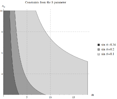
Figure 1: The $(\sin\theta,fR,N_{tc})$ parameter region allowed by the $S$ parameter restraints.

The $S$ parameter gives some restraint on a $(\sin\theta,fR,N_{tc})$ plane, see Fig. 1. The larger the value of $\sin\theta$ the smaller the allowed region for $fR$ and $N_{tc}$, though we only consider $\sin\theta\leq 0.34$ following the present bounds on the misalignment in the Minimal Composite Higgs Model Aad et al. (2015) (assuming the coupling of the Higgs to gauge bosons being $\kappa_{V}=\sqrt{1-\sin^{2}\theta}$).

We get no information about $\kappa^{2}$, the parameter that sets the overall scale of the masses, from the electroweak oblique parameters. However, through the $W$ mass of Eqn. (82) we can relate it to the EWSB scale $v=246$ GeV. Eqn. (82) as well contains the UV regulator

$$\varepsilon=\frac{1}{\Lambda_{\text{cut-off}}}\simeq\frac{1}{4\pi F}=\frac{\sin\theta}{4\pi v}.$$ (104)

The cut-off is assumed to be $4\pi F$ as this is the range of validity of the effective theory of vector and scalar composite resonances that has been assumed in the bottom-up holographic approach. Thus, we get an implicit equation defining the $\kappa^{2}$ parameter:

$$\frac{v^{2}}{\sin^{2}\theta}+\frac{5}{256\pi^{2}}4\kappa^{2}N_{tc}(fR)^{2}\left(\ln\frac{4\kappa^{2}\sin^{2}\theta}{64\pi^{2}v^{2}}+2\gamma_{E}+\psi\left(1+\frac{(fR)^{2}}{32}\right)\right)=0.$$ (105)

Table 1: Different predictions of the minimal vector masses for $\sin\theta=0.2$ and $0.3$.

$\sin\theta$	$N_{tc}$	$fR$	$M_{\ast}=M_{V}(0)$, TeV	$M_{A}(0)$, TeV	$\sim N_{max}$
$0.2$	$2$	$9.0$	$1.02$	$1.91$	$290$
$0.2$	$3$	$5.8$	$1.27$	$1.81$	$188$
$0.2$	$4$	$4.5$	$1.39$	$1.78$	$156$
$0.2$	$10$	$2.4$	$1.61$	$1.75$	$117$
$0.3$	$2$	$4.1$	$1.61$	$1.99$	$51$
$0.3$	$3$	$3.1$	$1.73$	$1.97$	$45$
$0.3$	$4$	$2.6$	$1.78$	$1.96$	$42$
$0.3$	$10$	$1.5$	$1.88$	$1.95$	$38$

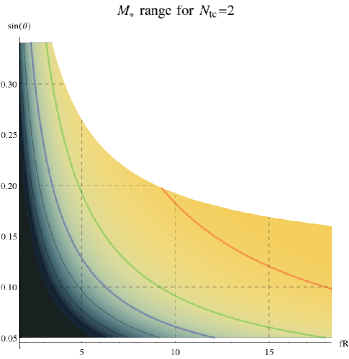
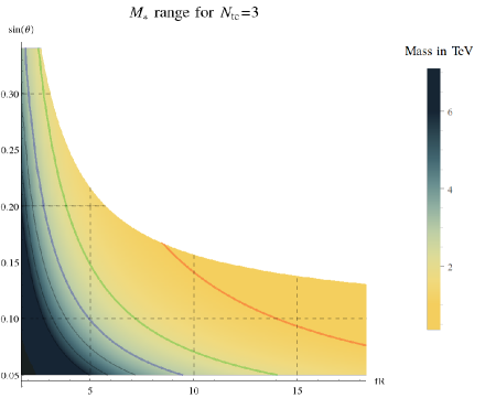
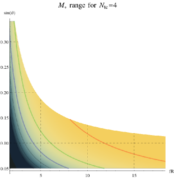
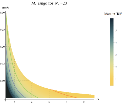
Figure 2: The density plots of $M_{*}$ for different values of $N_{tc}$. The coloured curves represent the lines of constant $M_{*}$: the red one - $M_{*}=1$ TeV, the green one - $M_{*}=2$ TeV, the blue one - $M_{*}=3$ TeV and successive black curves for higher integer values. The white area represents the sector prohibited by the $S$ bound.

In addition, we have a connection between the UV cut-off $\varepsilon$ and the maximum number of resonances $N_{max}$ from which one can express $\kappa^{2}$:

$$4\kappa^{2}=\frac{64\pi^{2}v^{2}}{\sin^{2}\theta}N_{max}^{-1}e^{-2\gamma_{E}}.$$ (106)

We consider Eqn. (105) as a problem of finding a minimal value of a characteristic mass $M_{\ast}=\sqrt{4\kappa^{2}}$ depending on values of the parameters $(\sin\theta,fR,N_{tc})$ from a region allowed by the $S$ parameter. We find that for fairly large values of $\sin\theta\simeq 0.2\div 0.34$ one can get $M_{\ast}$ of the order $\simeq 1\div 2$ TeV and higher. See Table 1 for the lowest values of $M_{V}(0)$ and $M_{A}(0)$ in the allowed region of $(fR,N_{tc})$. The lowest values of $M_{\ast}$ come from saturating the $S$ bound with a value of $fR$ for a given fixed $N_{tc}$. The results presented in Table 1 correspond to the current maximum positive value of $S$. Should it be found that $S$ is $n$ times smaller, our estimates for $M_{\ast}$ become roughly $n$ times larger.

The predictions for the characteristic mass $M_{*}$ for a wide range of parameters are depicted at Fig. 2. First, we note that a broad variety of masses is allowed even considering the constraints of oblique corrections. The region below $1$ TeV starts for rather large values of $fR$ making them experimentally disfavoured unless the misalignment angle is extremely small. In addition, a large $fR$ leads to a large splitting between vector fields aligned in different (unbroken and broken) directions. Mind also that in a tower of resonances of one type we have a square root growth with the number of a resonance, thus for a rather small value of $M_{*}$ we have a tower with several low-lying states, like $M_{V}(n)=\{1,1.4,1.7,2,...\}$ TeV.

Some general tendencies may be followed from Fig. 2 as well. Consider the parameter space $(\sin\theta,fR,N_{tc})$ and fix any two values, then the growth of the third parameter results in lower $M_{*}$. Though unlimited growth in $fR$ results in unlikely small masses, the higher values of other two parameters soon face the upper experimental limit of the $S$ parameter.

We may imagine another free parameter of the theory considering a breaking pattern $SO(N)\rightarrow SO(N-1)$ with an arbitrary $N$. A generalization from the particular case $N=5$ discussed previously is straightforward. The minimality is lost of course, and many more states appear in the model. Still it is interesting to estimate how the value of $N$ affects the masses of the vector resonances. Generally, the $S$ parameter has a linear dependence on $N$ and becomes proportionally more constraining at $N>5$, bringing the $S$ boundary to lower values of $fR$. That results in higher values for the characteristic mass $M_{*}$, but the resonances of unbroken and broken sector are closer in mass. For instance, having $SO(9)\rightarrow SO(8)$ breaking pattern Bertuzzo et al. (2013) and $N_{tc}=3$ we may get the minimal values $M_{V}(0)=1.49$ TeV and $M_{A}(0)=1.76$ TeV for $\sin\theta=0.2$ and $M_{V}(0)=1.83$ TeV and $M_{A}(0)=1.95$ TeV for $\sin\theta=0.3$. However, $M_{*}$ cannot experience an uncontrollable growth, the saturation is faced as soon as $fR$ is constrained by the $S$ to be small enough to have the masses in two channels almost equal. Remarkably, though occurring for an unrealistically high degree of the global group, these extreme values are rather moderate: $M_{V}(0)\simeq M_{A}(0)=1.7$ TeV for $\sin\theta=0.2$ and $M_{V}(0)\simeq M_{A}(0)=1.9$ TeV for $\sin\theta=0.3$, independently of the $N_{tc}$ value.

IX Conclusions

In this work we have reported on a bottom-up holographic study of the minimal composite Higgs model based on the breaking pattern $SO(5)\to SO(4)$ and a gauge group misaligned with the unbroken group. The fundamental degrees of freedom are assumed to be scalars living in some representation of $SO(5)$ and bound together by some unspecified strong dynamics which is also assumed to trigger the breaking of the global symmetry. Extending our results to larger orthogonal groups would be straightforward. A possible extension in another direction would be to consider Majorana fermions as fundamental degrees of freedom.

The main motivation for this analysis is to give plausible predictions for the spectrum of spin one and spin zero resonances taking into account all the existing experimental constraints at present. It has been argued elsewhere that the $S$ parameter bounds force the lightest vector resonances to be at least in the 2 TeV region. Not much is known about possible scalar resonances so far.

The soft wall 5D holographic model we have used is inspired by the effective models of QCD and consists in a generalized sigma model coupled both to the composite resonances and to the SM gauge bosons. The 5D model depends on three functions that parametrize our ansatz: the dilaton $z$-profile (a feature common to all soft wall holographic models), and two functions $f(z)$ and $b(z)$ that describe the generalized sigma model with an additional soft explicit breaking. There are several interesting features present in the resulting spectrum: one is that Goldstone bosons can be made exactly massless. Another one is that in the unbroken sector vectors and scalars are degenerate in mass; not so for the states living in the broken sector.

The two Weinberg sum rules hold but in a way only in a formal sense as the sum over resonances has to be cut off (it is logarithmically divergent). The holographic effective theory has a built-in cut-off that is related to the maximum number of resonances included. However, adhering to this cut-off it is possible to derive relations involving resonance decay constants and masses. Yet, the fact that the sum rules are divergent implies that they are not saturated at all by just the first resonance, as is the case in QCD.

We proceed to determining the minimal set of input parameters by including the short distance constraints resulting from comparison with perturbation theory in the vector and scalar channels and include the constraints coming from the $W$ mass, the $S$ parameter and the existing bounds on $\sin\theta$. This allows us to derive masses for the first composite resonances. It is not difficult to find areas in the parameter space where a resonance between 1 and 2 TeV is easily accommodated, even lighter in the lowest range of values for $\sin\theta$ and for large values of $fR$, even though this limit looks somewhat unnatural and fine-tuned. Large values of $fR$ also lead to a large mass splitting between the broken and unbroken sectors.

Appendix A Some properties of the confluent hypergeometric functions

The confluent hypergeometric equation has the general form:

$$xf^{\prime\prime}(x)+(c-x)f^{\prime}(x)-af(x)=0.$$ (107)

Solutions of this equation depend crucially on the value of the $a$ and $c$ parameters. Here we provide a brief overlook of the properties of the confluent hypergeometric equation, focusing on the dependence on the different integer values of the $c$ parameter Erdélyi (1953).

For the positive integer values $c=1,2,3,...$ we have

$$f(x)=C_{1}\ {}_{1}F_{1}(a,c;x)+C_{2}\Psi(a,c;x),$$ (108)

where $\ {}_{1}F_{1}(a,c;x)$ is called the Kummer’s (confluent hypergeometric) function and $\Psi(a,c;x)$ - the Tricomi’s (confluent hypergeometric) function.

However, all the cases mentioned in the paper lie in the region of the non-positive integer $c$, for which one of the expected solutions, ${}_{1}F_{1}(a,c;x)$, does not exist, because it has poles at $c=0,-1,-2,...$. In the same time the Tricomi’s function can be analytically continued to any integer $c$. Nevertheless, the fundamental system of solutions is rich enough and we are able to choose another two solutions:

$$f(x)=C_{1}x^{1-c}\ _{1}F_{1}(a-c+1,2-c;x)+C_{2}\Psi(a,c;x).$$ (109)

Mark that the Tricomi’s function exhibits a logarithmic behaviour for all integer $c$. Specifically for the case $c=1-n,\ n=0,1,2,...$ one can write:

$$\Psi(a,1-n;x) =\frac{(n-1)!}{\Gamma(a+n)}\sum\limits_{r=0}^{n-1}\frac{(a)_{r}x^{r}}{(1-n)_{r}r!}+\frac{(-1)^{n-1}}{n!\Gamma(a)}\bigg{(}\ _{1}F_{1}(a+n,n+1;x)x^{n}\ln x+$$

$$+\left.\sum\limits_{r=0}^{\infty}\frac{(a+n)_{r}}{(n+1)_{r}}[\psi(a+n+r)-\psi(1+r)-\psi(1+n+r)]\frac{x^{n+r}}{r!}\right),$$ (110)

here the Pochhammer symbol is $(a)_{n}=1\cdot a\cdot(a+1)...(a+n-1)=\Gamma(a+n)/\Gamma(a)$, $\psi(a)$ is the digamma function; and the first sum is absent for the case $n=0$. There exists also a useful equation relating the Tricomi’s functions of different arguments:

$$\Psi(a,c;x)=x^{1-c}\Psi(a-c+1,2-c;x).$$ (111)

The Kummer’s function being an infinite series solution $\ {}_{1}F_{1}(a,c;x)=\sum\limits_{n=0}^{\infty}\frac{(a)_{n}}{(c)_{n}}\frac{x^{n}}{n!}$ has a natural connection with the Laguerre polynomials (for integer $n>0,\ m>0$):

$$L_{n}^{m}(x)=\frac{(m+1)_{n}}{n!}\ _{1}F_{1}(-n,m+1,x).$$ (112)

Appendix B Large $Q^{2}$ expansion of the correlator $\Pi_{LR}$

Here we perform the large $Q^{2}$ expansion of $\Pi_{LR}$ using the infinite series representation of the digamma function $\psi(1+z)=-\gamma_{E}+\sum\limits_{n=1}^{\infty}\frac{z}{n(n+z)}$ valid for $z\neq-1,-2,...$ (derived from the series representation of the $\Gamma$-function) Erdélyi (1953), for the particular ones from Eqn. (85) we have:

$$\lim\limits_{Q^{2}\rightarrow\infty}\psi\left(\frac{Q^{2}}{4\kappa^{2}}+1\right)=-\gamma_{E}+\sum\limits_{n=0}^{\infty}\frac{1}{n+1}\sum\limits_{k=0}^{\infty}\left(\frac{-M^{2}_{V}(n)}{Q^{2}}\right)^{k},$$ (113)

$$\lim\limits_{Q^{2}\rightarrow\infty}\psi\left(\frac{Q^{2}}{4\kappa^{2}}+1+\frac{(g_{5}Rf)^{2}}{2k_{s}}\right)=-\gamma_{E}+\left(1+\frac{2\kappa^{2}(g_{5}Rf)^{2}}{k_{s}Q^{2}}\right)\sum\limits_{n=0}^{\infty}\frac{1}{n+1}\sum\limits_{k=0}^{\infty}\left(\frac{-M^{2}_{A}(n)}{Q^{2}}\right)^{k},$$

where for $k=0$ we have $\lim\limits_{N\rightarrow\infty}\sum\limits_{n=1}^{N}\frac{1}{n}=\lim\limits_{N\rightarrow\infty}H_{N}=\ln N+\gamma_{E}+\mathcal{O}(1/N)$, $H_{N}$ being the N-th harmonic number.

Substitution in Eqn. (85) yields order by order for $\Pi_{LR}(Q^{2})/Q^{2}$:

$$\left(\frac{1}{Q^{2}}\right)^{0}:\quad\sin^{2}\theta\frac{R}{2g_{5}^{2}}\left(\sum\limits_{n=0}^{\infty}\frac{1}{n+1}-\sum\limits_{n=0}^{\infty}\frac{1}{n+1}\right);$$ (114)

$$\left(\frac{1}{Q^{2}}\right)^{1}:\quad 4\kappa^{2}\sin^{2}\theta\frac{R}{2g_{5}^{2}}\sum\limits_{n=0}^{\infty}(1-1)-\sin^{2}\theta(fR)^{2}\kappa^{2}\frac{R}{k_{s}}\left(\ln\varepsilon^{2}\kappa^{2}+\gamma_{E}+\sum\limits_{n=0}^{\infty}\frac{1}{n+1}\right);$$ (115)

$$\left(\frac{1}{Q^{2}}\right)^{2}:\quad 4\kappa^{4}\sin^{2}\theta(fR)^{2}\frac{R}{k_{s}}\sum\limits_{n=0}^{\infty}(1-1).$$ (116)

Considering that $1$ and $-1$ come together for any $n$, as well as the fractions in the difference between harmonic sums, we set these terms to zeros (certainly 0 for a finite sum) and get:

$$\frac{\Pi_{LR}(Q^{2})}{Q^{2}}=-\sin^{2}\theta(fR)^{2}\kappa^{2}\frac{R}{k_{s}}\left(\ln\varepsilon^{2}\kappa^{2}+\gamma_{E}+\sum\limits_{n=0}^{\infty}\frac{1}{n+1}\right)\frac{1}{Q^{2}}+\mathcal{O}\left(\frac{1}{Q^{6}}\right).$$ (117)

In our discussion of subtraction constants in Section V the term in brackets has been taken to be zero as the infinite sum is replaced with the one up to $N_{max}$. Thus we show that the terms $1/Q^{2}$ and $1/Q^{4}$ are absent as long as $N_{max}<\infty$.

Appendix C Loop diagrams in the fundamental theory

We presume that the fundamental theory is defined by an $SO(5)$-invariant Lagrangian:

$$\mathcal{L}_{str.int.}=\frac{1}{2}\partial_{\mu}s_{\alpha\beta}\partial^{\mu}s^{\top}_{\beta\alpha}-\frac{1}{2}m^{2}s_{\alpha\beta}s^{\top}_{\beta\alpha}+\text{higher order terms},$$ (118)

where $s_{\alpha\beta}$ are in a general 25-plet of $SO(5)$. The propagator of $s_{\alpha\beta}$ is given then by:

$$i\Delta^{\alpha\beta\alpha^{\prime}\beta^{\prime}}=\frac{i\delta^{\alpha\alpha^{\prime}}\delta^{\beta\beta^{\prime}}}{p^{2}-m^{2}},$$ (119)

and the vertices are defined by the source-operator terms of Eqns. (14) and (16). Given this we can compute the leading order diagrams for the scalar and vector two-point functions.

We begin with considering the scalar two-point function in terms of the fundamental fields:

$$\int d^{4}xd^{4}ye^{-iq(x-y)}\langle iT^{a}_{\alpha\beta}s_{\beta\gamma}s_{\gamma\alpha}(x)\ \cdot\ iT^{b}_{\alpha^{\prime}\beta^{\prime}}s_{\beta^{\prime}\gamma^{\prime}}s_{\gamma^{\prime}\alpha^{\prime}}(y)\rangle=$$

$$=i^{2}\left(-5N_{tc}\operatorname{Tr}T^{a}T^{b}\right)\int\frac{d^{4}k}{(2\pi)^{4}}\frac{1}{(k+q)^{2}-m^{2}}\frac{1}{k^{2}-m^{2}}.$$ (120)

As is mentioned in Section V in the large $Q^{2}$ limit the leading logarithmic behaviour of the loop diagram corresponds to the one of $\Pi_{S}(Q^{2})$:

$$\delta^{ab}\Pi_{S}(Q^{2})\sim 5\operatorname{Tr}T^{a}T^{b}\frac{N_{tc}}{16\pi^{2}}\ln Q^{2},$$

giving the coefficient

$$\frac{k_{s}}{R}=\frac{64\pi^{2}}{5N_{tc}},$$ (121)

where “$N_{tc}$” signifies the degree of the representation of the gauge group under which the fundamental scalar fields transform (exactly $N_{tc}$ in case of the fundamental representation of $SU(N_{tc})$).

For the vector two-point function we get:

$$\int d^{4}xd^{4}ye^{-iq(x-y)}\langle i[T^{A},s]_{\alpha\beta}\partial^{\mu}s_{\alpha\beta}(x)\ \cdot\ i[T^{B},s]_{\alpha^{\prime}\beta^{\prime}}\partial^{\nu}s_{\alpha^{\prime}\beta^{\prime}}(y)\rangle=$$

$$=\left(10N_{tc}\operatorname{Tr}T^{A}T^{B}\right)\int\frac{d^{4}k}{(2\pi)^{4}}\frac{ik^{\mu}iq^{\nu}}{((k+q)^{2}-m^{2})(k^{2}-m^{2})}.$$ (122)

Taking the large $Q^{2}$ limit one may compute the leading logarithmic coefficient of the vectorial two-point functions ($\Pi_{unbr}$ and $\Pi_{br}$). However, we do not get the full transverse structure (only $q^{\mu}q^{\nu}$ term) as the interaction considered does not come from a Lorentz-invariant term in the Lagrangian. We miss here a coupling of a kind $ssA_{\mu}A^{\mu}$, which would have appeared had we considered real gauging in the fundamental theory. As this vertex could only contribute to the $\eta_{\mu\nu}$ part of $\Pi_{\mu\nu}$ and leaves $q^{\mu}q^{\nu}$ term unchanged we do not need any further computations to fix the leading $\ln Q^{2}$ coefficient:

$$\delta^{AB}\Pi^{\mu\nu}(Q^{2})\sim q^{\mu}q^{\nu}\left(-10\operatorname{Tr}T^{A}T^{B}\right)\frac{N_{tc}}{16\pi^{2}}\ln Q^{2}.$$

Thus, we get another coefficient fixed:

$$\frac{g_{5}^{2}}{R}=\frac{4\pi^{2}}{5N_{tc}}.$$ (123)