Neutrinophilic two Higgs doublet model
with $U(1)$ global symmetry

Abstract

We propose a neutrinophilic two-Higgs-doublet model, where the vacuum expectation value (VEV) of the second Higgs doublet is only induced at one-loop level via several neutral fermions. Thus, the masses of active neutrinos arising from the Higgs doublets are naturally small via such a tiny VEV. We discuss various phenomenology of the model, including the neutrino masses and oscillations, bounds on non-unitarity, lepton-flavor violations, the oblique parameters, the muon anomalous magnetic moment, the GeV-scale sterile neutrino candidate arising from the tiny VEV, and collider signatures. We finally discuss the possibility of detecting the sterile neutrino suggested in the experiment of Future Circular Collider (FCC).

I Introduction

Two-Higgs-doublet models (THDM) are regarded as the simplest extensions of the standard model (SM) by adding one more doublet Higgs field to the Higgs sector hunter . It is the most often studied model because of its rich phenomenology and accommodation of the Higgs sector of supersymmetric models. Nevertheless, THDM’s do not have enough matter contents to accommodate the small neutrino mass, at least in its simplest versions, conventionally dubbed as Types I, II, III, and IV.

Here we introduce an additional $U(1)$ global symmetry with a set of exotic fermions and a singlet Higgs field, beyond the THDM. Among the exotic fermions, there are Dirac and Majorana types. The first Higgs doublet field $\Phi_{1}$ is chosen to be the SM-like Higgs doublet while the second one $\Phi_{2}$ to be inert at tree level. Yet, a tiny vacuum expectation value (VEV) is generated at loop level for the second doublet, which is then used to explain the small neutrino mass. Such a setup can explain the small neutrino mass without invoking extremely small Yukawa couplings.

In this work, in addition to showing that the model can explain neutrino mass and oscillation pattern, and non-unitarity bound, we also show that it can be consistent with existing limits on the lepton-flavor violations and the oblique parameters. Furthermore, we can have heavier sterile neutrinos of mass ${\cal O}(0.1\sim 10)$ GeV, which are induced by the tiny VEV. Since the model also involves some exotic particles at TeV, we briefly describe the signatures that we can expect at the LHC.

This paper is organized as follows. In Sec. II, we describe the details of the model. In Sec. III, we study the phenomenology and constraints of the model, in particular, the derivations for the formulas of lepton-flavor violations, muon anomalous magnetic dipole moment ($g-2$), and the oblique parameters. In Sec. IV, we present the numerical analysis of the model. We conclude and discuss in Sec. V.

II Model setup

	Fermions						Bosons
Fermions	$L_{L}$	$e_{R}$	$L^{\prime}$	$N_{R_{0}}$	$N_{1}$	$N_{R_{2}}$	$\Phi_{1}$	$\Phi_{2}$	$\varphi$
$SU(2)_{L}$	$\bm{2}$	$\bm{1}$	$\bm{2}$	$\bm{1}$	$\bm{1}$	$\bm{1}$	$\bm{2}$	$\bm{2}$	$\bm{1}$
$U(1)_{Y}$	$-\frac{1}{2}$	$-1$	${-\frac{1}{2}}$	$0$	$0$	$0$	$\frac{1}{2}$	$\frac{1}{2}$	$0$
$U(1)$	$-1$	$-1$	$-\frac{1}{5}$	$0$	$-\frac{1}{5}$	$-\frac{2}{5}$	$0$	$\frac{3}{5}$	$\frac{1}{5}$

Table 1: Field contents of fermions and their charge assignments under $SU(2)_{L}\times U(1)_{Y}\times U(1)$, where each of the flavor index is abbreviated.

In this section, we describe the neutrinophilic model in detail, including the bosonic sector, fermion sectors, and the scalar potential. First of all, we introduce an additional $U(1)$ global symmetry. All the fermionic and bosonic contents and their assignments are summarized in Table 1. Notice here that the numbers of family for all exotic fermions, except for $N_{R_{0}}$ (two families), are three in order to reproduce the neutrino oscillation data, and $L^{\prime}$ and $N_{1}$ are Dirac-type fermions, while $N_{R_{0}}$ and $N_{R_{2}}$ are the Majorana fermions.

For the scalar sector with nonzero VEVs, we introduce two $SU(2)_{L}$ doublet scalars $\Phi_{1}$ and $\Phi_{2}$, and an $SU(2)_{L}$ singlet scalar $\varphi$. Here $\Phi_{1}$ is supposed to be the SM-like Higgs doublet, while $\Phi_{2}$ is supposed to be an inert doublet at tree level. After spontaneous breaking of $U(1)$ via $\varphi$, the VEV of $\Phi_{2}$ is induced at the one-loop level via exotic fermions. Thus, a tiny VEV can theoretically be realized, which could be natural to generate the tiny neutrino masses.

In the framework of neutrinophilic THDM’s, several scenarios have been considered in literature. For example, a tiny VEV is induced by bosonic loops at one-loop level with a global $U(1)_{B-L}$ symmetry and thus the active neutrinos are expected to be Dirac fermions  Kanemura:2013qva . The work in Ref. Nomura:2017ezy had considered a tiny VEV generated at bosonic one-loop level with a $U(1)_{R}$ gauge symmetry, and all the light SM fermion masses are induced via this tiny VEV while the neutrino masses are induced at two-loop level as Majorana fermions. Another work in Ref Wang:2016vfj had considered the scenario in neutrinophilic THDM with a $U(1)_{L}$ global symmetry, in which neutrino masses are induced at tree-level as Majorana fermions and they also discussed the possibility of explaining the anomalous X-ray line.

II.1 Yukawa interactions and scalar sector

Yukawa Lagrangian: With the current field contents and symmetries, the renormalizable Lagrangian in the leptonic sector is given by

$$-{\cal L}_{L} =(y_{\ell})_{ii}\bar{L}_{L_{i}}\Phi_{1}e_{R_{i}}+f_{ij}\bar{L}^{\prime}_{L_{i}}\tilde{\Phi}_{1}N_{R_{1j}}+f^{\prime}_{ij}\bar{N}_{L_{i}}L^{\prime}_{R_{j}}\Phi_{1}+g_{ij}\bar{L}^{\prime C}_{R_{i}}\Phi_{2}N_{R_{2j}}+(y_{L_{2}})_{ij}\bar{L}_{L_{i}}\tilde{\Phi}_{2}N_{R_{2j}}$$

$$+(y_{N})_{ij}\bar{N}_{R_{2i}}N_{L_{1j}}\varphi+(y^{\prime}_{N})_{ia}\bar{N}_{L_{1i}}N_{R_{0a}}\varphi+(y^{\prime\prime}_{N})_{ia}\bar{N}_{R_{1i}}N^{C}_{R_{0a}}\varphi+(M_{D})_{ij}\bar{N}_{L_{1i}}N_{R_{1j}}$$

$$+(M_{0})_{aa}\bar{N}^{C}_{R_{0a}}N_{R_{0a}}+(M_{L^{\prime}})_{ii}\bar{L}^{\prime}_{L_{i}}L^{\prime}_{R_{i}}+{\rm c.c.},$$ (II.1)

where $(i,j)=1-3$, $a=1,2$, $\tilde{\Phi}_{1,2}\equiv(i\sigma_{2})\Phi_{1,2}^{*}$ with $\sigma_{2}$ being the second Pauli matrix, and the mass matrices in the last line are diagonal without loss of generality as well as $y_{\ell}$. 

II.2 Fermion Sector

First of all, we define the exotic fermion as follows:

$$L^{\prime}_{L(R)}\equiv\left[\begin{array}[]{c}N^{\prime}\\ E^{\prime-}\end{array}\right]_{L(R)},$$ (II.4)

then the mass eigenvalue of charged fermion is straightforwardly given by $M_{L^{\prime}}$ in Eq.(II.1). The mass matrix for the neutral exotic fermions is a $7\times 7$ block in basis of $\Psi\equiv[\nu_{L}^{C},N_{R_{0}},N_{R_{1}},N^{C}_{L_{1}},N_{R_{2}},N^{\prime}_{R},N^{\prime C}_{L}]$, and given by

$$M_{N}(\Psi)=\left[\begin{array}[]{ccccccc}{\bf 0_{3\times 3}}&{\bf 0_{3\times 2}}&{\bf 0_{3\times 3}}&{{\bf 0_{3\times 3}}}&{m_{D}}&{\bf 0_{3\times 3}}&{\bf 0_{3\times 3}}\\ {\bf 0_{2\times 3}}&M_{0}&M_{N_{3}}^{T}&M_{N_{2}}^{T}&{\bf 0_{2\times 3}}&{\bf 0_{2\times 3}}&{\bf 0_{2\times 3}}\\ {\bf 0_{3\times 3}}&M_{N_{3}}&{\bf 0_{3\times 3}}&M_{D}^{T}&{\bf 0_{3\times 3}}&{\bf 0_{3\times 3}}&M^{T}\\ {{\bf 0_{3\times 3}}}&M_{N_{2}}&M_{D}&{\bf 0_{3\times 3}}&M_{N_{1}}^{T}&M^{\prime}&{\bf 0_{3\times 3}}\\ {m_{D}^{T}}&{\bf 0_{3\times 2}}&{\bf 0_{3\times 3}}&M_{N_{1}}&{\bf 0_{3\times 3}}&m^{T}&{\bf 0_{3\times 3}}\\ {\bf 0_{3\times 3}}&{\bf 0_{3\times 2}}&{\bf 0_{3\times 3}}&M^{\prime T}&m&{\bf 0_{3\times 3}}&M_{L^{\prime}}\\ {\bf 0_{3\times 3}}&{\bf 0_{3\times 2}}&M&{\bf 0_{3\times 3}}&{\bf 0_{3\times 3}}&M_{L^{\prime}}^{T}&{\bf 0_{3\times 3}}\\ \end{array}\right],$$ (II.12)

where we define $m\equiv g_{ij}v_{2}/\sqrt{2}$, $m_{D}\equiv(y_{L_{2}})_{ij}v_{2}/\sqrt{2}$, $M\equiv f_{ij}v_{1}/\sqrt{2}$, $M^{\prime}\equiv f^{\prime}_{ij}v_{1}/\sqrt{2}$, $M_{N_{1}}\equiv(y_{N})_{ij}v^{\prime}/\sqrt{2}$, $M_{N_{2}}\equiv(y^{\prime}_{N})_{ia}v^{\prime}/\sqrt{2}$, $M_{N_{3}}\equiv(y^{\prime\prime}_{N})_{ia}v^{\prime}/\sqrt{2}$. Then this matrix is diagonalized by a $20\times 20$ unitary matrix $V_{N}$ as $M_{\psi_{\alpha}}\equiv(V_{N}M_{N}V_{N}^{T})_{\alpha}$ $(\alpha=1\sim 20)$, where $M_{\psi_{\alpha}}$ consists of the mass eigenvalues.

II.3 Scalar potential

In our model, the scalar potential is given by

$$V= \mu_{\varphi}^{2}|\varphi|^{2}+\lambda_{\varphi}|\varphi|^{4}+\sum_{i=1,2}\lambda_{\varphi\Phi_{i}}|\varphi|^{2}|\Phi_{i}|^{2}$$

$$+\mu_{11}^{2}|\Phi_{1}|^{2}+\mu_{22}^{2}|\Phi_{2}|^{2}+\frac{\lambda_{1}}{2}|\Phi_{1}|^{4}+\frac{\lambda_{2}}{2}|\Phi_{2}|^{4}+\lambda_{3}|\Phi_{1}|^{2}|\Phi_{2}|^{2}+\lambda_{4}|\Phi_{1}^{\dagger}\Phi_{2}|^{2},$$ (II.13)

where we have chosen some parameters in the potential such that $\langle\Phi_{2}\rangle\equiv v_{2}/\sqrt{2}=0$ at tree level, while $\varphi=\frac{1}{\sqrt{2}}(v^{\prime}+\varphi_{R}+iG)$ with $v^{\prime}\neq 0$ and $\langle\Phi_{1}\rangle\equiv v_{1}/\sqrt{2}\neq 0$. Here $\varphi_{R}$ is assumed to be the mass eigenstate that suggests the mass of $\varphi_{R}$ is larger than the other mass eigenvalues. $G$ is the physical Goldstone boson (GB) that does not mix with other particles. To achieve the inert $\Phi_{2}$, we impose the inert conditions as follows:

$$0<\lambda_{2},\quad 0\leq 2\mu_{22}^{2}+(\lambda_{3}+\lambda_{4})v_{1}^{2}+\lambda_{\varphi\Phi_{2}}v^{\prime 2}.$$

Figure 1: 1 loop induced 5 dimensional operator

A five-demensional operator $\lambda_{5}\varphi^{3}\Phi_{2}^{\dagger}\Phi_{1}$ can be generated at one-loop level as shown in Fig.1. The formula is given by

$$\lambda_{5} =\sum_{a=1}^{20}\frac{4M_{L^{\prime}_{j}}}{\left(4\pi\right)^{2}}\left[f_{i,m}g_{i,j}\left(y_{N}\right)_{j,k}\left(y^{\prime}_{N}\right)_{k,l}\left(y^{\prime\prime}_{N}\right)_{m,l}\right]F\left(4,1,\{M_{0_{i}}^{2},M_{L^{\prime}_{j}}^{2},M_{D_{k}}^{2},M_{D_{l}}^{2}\}\right),$$ (II.14)

where the explicit expression for $F\left(4,1,\{M_{0_{i}},M_{L^{\prime}_{j}},M_{D_{k}},M_{D_{l}}\}\right)$ is given in Appendix A. After the spontaneous symmetry breaking, an effective mass term $\mu_{12}^{2}\Phi^{\dagger}_{2}\Phi_{1}=\frac{\lambda_{5}v^{\prime 3}}{2\sqrt{2}}\Phi_{2}^{\dagger}\Phi_{1}$ is obtained. The resultant scalar potential in the THDM Higgs sector is given by

$$V_{THDM}= \mu_{12}^{2}(\Phi_{1}^{\dagger}\Phi_{2}+{\rm c.c.})+\mu_{11}^{\prime 2}|\Phi_{1}|^{2}+\mu_{22}^{\prime 2}|\Phi_{2}|^{2}$$

$$+\frac{\lambda_{1}}{2}|\Phi_{1}|^{4}+\frac{\lambda_{2}}{2}|\Phi_{2}|^{4}+\lambda_{3}|\Phi_{1}|^{2}|\Phi_{2}|^{2}+\lambda_{4}|\Phi_{1}^{\dagger}\Phi_{2}|^{2},$$ (II.15)

where $\mu_{11(22)}^{\prime 2}\equiv\mu_{11(22)}^{2}+\lambda_{\varphi\Phi_{1(2)}}v^{\prime 2}/2$, $\langle\Phi_{i}\rangle\equiv v_{i}/\sqrt{2}$ ($i=1-2$) and we choose $\mu_{12}^{2}$ to be negative, while $\mu_{11}^{2}$ to be positive, and assume that $v_{2}/v^{\prime}\ll 1$. Taking $v_{2}/v_{1}\ll 1$, we finally obtain the formula for the VEV of $\Phi_{2}$ as

$$v_{2}\approx\frac{2v_{1}\mu_{12}^{2}}{2\mu_{22}^{\prime 2}+v_{1}^{2}(\lambda_{3}+\lambda_{4})}.$$ (II.16)

Including their VEVs, the scalar fields are parameterized as

$$\Phi_{1}=\left[\begin{array}[]{c}h_{1}^{+}\\ \frac{v_{1}+h_{1}+ia_{1}}{\sqrt{2}}\end{array}\right],\quad\Phi_{2}=\left[\begin{array}[]{c}h_{2}^{+}\\ \frac{v_{2}+h_{2}+ia_{2}}{\sqrt{2}}\end{array}\right].$$ (II.21)

After the spontaneous symmetry breaking, the neutral scalar bosons $\varphi_{R}$ and $h_{1}$ mix each other to form mass eigenstates. Note that the VEV of the second Higgs doublet is too small for a sizeable mixing with $h_{2}$. The pseudoscalar components and the charged components are rotated to give the zero-mass Goldstone bosons and the physical pseudoscalar Higgs boson and charged Higgs boson, respectively. They are given in the following expressions:

$$\text{Diag.}(m_{H_{1}^{0}}^{2},m_{H_{2}^{0}}^{2})=O_{H}m^{2}(\varphi_{R},h_{1})O_{H}^{T},$$

$$\text{Diag.}(m_{Z^{0}}^{2},m_{A^{0}}^{2})=O_{I}m^{2}(a_{1},a_{2})O_{I}^{T},$$

$$\text{Diag.}(m_{\omega^{\pm}}^{2},m_{H^{\pm}}^{2})=O_{C}m^{2}(h_{1}^{\pm},h_{2}^{\pm})O_{C}^{T},$$ (II.22)

where $O_{H,C,I}$ denotes the mixing matrices which diagonalize the mass matrices accordingly. Here $Z^{0}$ and $\omega^{\pm}$ are zero-mass Goldstone bosons to be absorbed as the longitudinal component of the neutral SM gauge boson $Z$ and charged gauge boson $W^{\pm}$ respectively. The mass matrices in the right-hand side of Eq. (II.3) are given by the parameters in the scalar potential. For neutral CP-even components we obtain

$$m^{2}(\varphi_{R},h_{1})\sim\left[\begin{array}[]{cc}2\lambda_{\varphi}v^{\prime 2}&v_{1}v^{\prime}\lambda_{\varphi\Phi_{1}}\\ v_{1}v^{\prime}\lambda_{\varphi\Phi_{1}}&2\lambda_{1}v_{1}^{2}-\frac{v_{2}\mu^{2}_{12}}{v_{1}}\\ \end{array}\right],$$ (II.25)

where $H_{1}^{0}(\equiv h_{SM})$ is the SM-like Higgs in our notation, and $h_{2}$ does not mix in the limit of $\mu_{12},v_{2}\ll v_{1},v_{\varphi}$; $m_{h_{2}}^{2}\sim 2\lambda_{2}v_{2}^{2}-\frac{v_{2}\mu^{2}_{12}}{v_{2}}$. We also obtain the mass matrices for CP-odd and charged components as

$$m^{2}(a_{1},a_{2})=\left[\begin{array}[]{cc}-\frac{v_{2}\mu_{12}^{2}}{v_{1}}&\mu_{12}^{2}\\ \mu_{12}^{2}&-\frac{v_{1}\mu_{12}^{2}}{v_{2}}\\ \end{array}\right],\ m_{A^{0}}^{2}=-\frac{(v_{1}^{2}+v_{2}^{2})\mu_{12}^{2}}{v_{1}v_{2}},$$ (II.28)

$$m^{2}(h_{1}^{\pm},h_{2}^{\pm})=\left[\begin{array}[]{cc}-\frac{v_{2}(\lambda_{4}v_{1}v_{2}+2\mu_{12}^{2})}{2v_{1}}&\frac{\lambda_{4}v_{1}v_{2}}{2}+\mu_{12}^{2}\\ \frac{\lambda_{4}v_{1}v_{2}}{2}+\mu_{12}^{2}&-\frac{v_{1}(\lambda_{4}v_{1}v_{2}+2\mu_{12}^{2})}{2v_{2}}\\ \end{array}\right],\ m_{H^{\pm}}^{2}=-\frac{(v_{1}^{2}+v_{2}^{2})(\lambda_{4}v_{1}v_{2}+2\mu_{12}^{2})}{2v_{1}v_{2}}.$$ (II.31)

Here we explicitly show the $2\times 2$ matrices; $O_{R},O_{C},O_{I}$, as

$$O_{R} \equiv\left[\begin{array}[]{cc}c_{\alpha}&s_{\alpha}\\ -s_{\alpha}&c_{\alpha}\\ \end{array}\right],\quad\quad O_{I}\equiv O_{C}=\left[\begin{array}[]{cc}c_{\beta}&s_{\beta}\\ -s_{\beta}&c_{\beta}\\ \end{array}\right],\quad s_{\beta}=\frac{v_{2}}{\sqrt{v_{1}^{2}+v_{2}^{2}}},$$ (II.36)

where $c_{\alpha(\beta)}\equiv\cos\alpha(\beta)$ and $s_{\alpha}(\beta)\equiv\sin\alpha(\beta)$, and we define $v\equiv\sqrt{v_{1}^{2}+v_{2}^{2}}$, $\tan\beta\equiv\frac{v_{2}}{v_{1}}$ which lead $v_{1}=v\cos\beta$ and $v_{2}=v\sin\beta$ as in the other THDMs. Since $v_{2}\ll v_{1}$ is achieved theoretically, $s_{\beta}\ll 1$ is realized. Also $s_{\alpha}$ is written in terms of the elements of $m^{2}(\varphi_{R},h_{1})$, which is restricted by the current experimental data at LHC $s_{\alpha}\lesssim 0.3$. Note that there is an advantage of introducing fermions inside the loop instead of bosons Kanemura:2013qva ; Nomura:2017ezy , because of the positivity of the fermion-loop contributions to the pure quartic couplings. Hence the vacuum stability can easily be realized Cheung:2016ypw .

III Phenomenology and Constraints

III.1 Neutrino masses and Oscillations

The charged-lepton mass is given by $m_{\ell}=y_{\ell}v/\sqrt{2}$ after the electroweak symmetry breaking, where $m_{\ell}$ is assumed to be the mass eigenstate. Let us redefine the neutral mass matrix $M_{N}$, its mixing matrix $V_{N}$ and mass eigenvalues $M_{\psi}$ as two by two block-mass matrices for the convenience of discussing the non-unitarity of leptonic mixing matrix Agostinho:2017wfs :

$$M_{N} =\left[\begin{array}[]{cc}0_{3\times 3}&m_{3\times 17}\\ m^{T}_{17\times 3}&M_{17\times 17}\\ \end{array}\right],\quad M_{\psi}=\left[\begin{array}[]{cc}d_{3\times 3}&0_{3\times 17}\\ 0^{T}_{17\times 3}&D_{17\times 17}\\ \end{array}\right],$$ (III.5)

$$V_{N} =\left[\begin{array}[]{cc}(V_{N})_{3\times 3}&0_{3\times 17}\\ 0^{T}_{17\times 3}&(V_{N})_{17\times 17}\\ \end{array}\right]\left[\begin{array}[]{cc}1_{3\times 3}&X^{\dagger}_{3\times 17}\\ X_{17\times 3}&1_{17\times 17}\\ \end{array}\right],\quad$$ (III.10)

where $(V_{N})_{3\times 3}$ and $d_{3\times 3}$ correspond, respectively, to the lepton-mixing matrix with non-unitarity, and mass eigenvalues of active neutrinos. With several steps, $X$ can be parametrized by

$$X=\pm i\sqrt{D^{-1}}{\cal O}\sqrt{d},$$ (III.11)

where ${\cal O}$ is an arbitrary $17\times 3$ matrix with 45 degrees of freedom, satisfying ${\cal O}^{T}{\cal O}=1_{3\times 3}$ but ${\cal O}{\cal O}^{T}\neq 1_{17\times 17}$. Next, consider the Hermitian matrix $X^{\dagger}X$ being diagonalized by a unitary $3\times 3$ mixing matrix $U$, i.e., $d_{X}^{2}\equiv U^{\dagger}X^{\dagger}XU$. Then the non-unitarity parameter $\eta$, which is defined by $(V_{N})_{3\times 3}\equiv(1-\eta)V_{MNS}$, should be smaller than the following bounds that arise from global constraints in Ref. Fernandez-Martinez:2016lgt

$$|2\eta|\simeq|V_{k}d_{X}^{2}V^{\dagger}_{k}|\lesssim\left[\begin{array}[]{ccc}2.5\times 10^{-3}&2.4\times 10^{-5}&2.7\times 10^{-3}\\ 2.4\times 10^{-5}&4.0\times 10^{-4}&1.2\times 10^{-3}\\ 2.7\times 10^{-3}&1.2\times 10^{-3}&5.6\times 10^{-3}\\ \end{array}\right],$$ (III.15)

$$V_{MNS}=\left[\begin{array}[]{ccc}{c_{13}}c_{12}&c_{13}s_{12}&s_{13}e^{-i\delta}\\ -c_{23}s_{12}-s_{23}s_{13}c_{12}e^{i\delta}&c_{23}c_{12}-s_{23}s_{13}s_{12}e^{i\delta}&s_{23}c_{13}\\ s_{23}s_{12}-c_{23}s_{13}c_{12}e^{i\delta}&-s_{23}c_{12}-c_{23}s_{13}s_{12}e^{i\delta}&c_{23}c_{13}\\ \end{array}\right]\left[\begin{array}[]{ccc}e^{i\alpha_{1}/2}&0&0\\ 0&e^{i\alpha_{2}/2}&0\\ 0&0&1\\ \end{array}\right],$$ (III.22)

where $V_{MNS}$ is the unitary $3\times 3$ lepton-mixing matrix that is observed, and $V_{k}\equiv(V_{N})_{3\times 3}U_{3\times 3}(\sqrt{1+d_{X}^{2}})_{3\times 3}$. In our numerical analysis, we implicitly satisfy this condition.  

In addition to the bounds on non-unitarity, we further impose the following ranges on

$$V^{\dagger}_{MNS}dV_{MNS}^{*}=\left[\begin{array}[]{ccc}0.0845-0.475&0.0629-0.971&0.0411-0.964\\ &1.44-3.49&1.94-2.85\\ &*&1.22-3.33\\ \end{array}\right]\times 10^{-11}\ {\rm GeV},$$ (III.26)

where we have used the following neutrino oscillation data at $3\sigma$ Forero:2014bxa in case of normal hierarchy (NH) given by 

$$0.278\leq s_{12}^{2}\leq 0.375,\ 0.392\leq s_{23}^{2}\leq 0.643,\ 0.0177\leq s_{13}^{2}\leq 0.0294,\ \delta\in[-\pi,\pi],$$

$$\sqrt{m_{\nu_{3}}^{2}-\frac{m_{\nu_{1}}^{2}+m_{\nu_{2}}^{2}}{2}}=(\sqrt{23.0}-\sqrt{26.5})\times 10^{-11}\ {\rm GeV},$$ (III.27)

$$\sqrt{m_{\nu_{2}}^{2}-m_{\nu_{1}}^{2}}=(\sqrt{0.711}-\sqrt{0.818})\times 10^{-11}\ {\rm GeV},$$ (III.28)

and the Majorana phases $\alpha_{1,2}$ taken to be $\alpha_{1,2}\in[-\pi,\pi]$.

In case of inverted hierarchy (IH) we also impose the following ranges at 3$\sigma$ confidential level Forero:2014bxa :

$$V^{\dagger}_{MNS}dV_{MNS}^{*} =\left[\begin{array}[]{ccc}1.00-5.00&0.00237-3.83&0.00256-3.94\\ &0.00279-3.08&0.365-2.60\\ &*&0.00500-3.30\\ \end{array}\right]\times 10^{-11}\ {\rm GeV},$$ (III.32)

$$0.403\leq s_{23}^{2}\leq 0.640,\ 0.0183\leq s_{13}^{2}\leq 0.0297,$$

$$\sqrt{\frac{m_{\nu_{1}}^{2}+m_{\nu_{2}}^{2}}{2}-m_{\nu_{3}}^{2}}=(\sqrt{22.0}-\sqrt{25.4})\times 10^{-11}\ {\rm GeV},$$ (III.33)

where the other values are same as the case of NH.

Process	$(i,j)$	Experimental bounds ($90\%$ CL)	References
$\mu^{-}\to e^{-}\gamma$	$(2,1)$	${BR}(\mu\to e\gamma)<4.2\times 10^{-13}$	TheMEG:2016wtm
$\tau^{-}\to e^{-}\gamma$	$(3,1)$	${Br}(\tau\to e\gamma)<3.3\times 10^{-8}$	Adam:2013mnn
$\tau^{-}\to\mu^{-}\gamma$	$(3,2)$	${BR}(\tau\to\mu\gamma)<4.4\times 10^{-8}$	Adam:2013mnn

Table 2: Summary of $\ell_{i}\to\ell_{j}\gamma$ process and the lower bound of experimental data.

III.2 Sterile neutrino

Due to two of the blocks in the mass matrix for neutral fermions, $m$ and $m_{D}$, in Eq. (II.12), we can have another three lighter neutral fermions in addition to the three active neutrinos. Hence the model can provide GeV-scale sterile neutrino(s) that have been studied in the Future Circular Collider (FCC) proposal Blondel:2014bra ; Alekhin:2015byh . Here let us focus on the lightest sterile fermion $\psi_{4}\equiv\nu_{s}$, and its mass is defined by $m_{\nu_{s}}$. Since the testability of FCC is provided in terms of $m_{\nu_{s}}$ and its mixing between $\nu_{s}$ and three active neutrinos Rasmussen:2016njh , we define its mixing as follows:

$$\theta_{s}\equiv\sqrt{|V_{4,1}|^{2}+|V_{4,2}|^{2}+|V_{4,3}|^{2}},$$ (III.34)

where $\theta_{s}$ depends on each of mass values in Eq. (II.12). The concrete analysis will be give in the next section.

III.3 Lepton Flavor Violations (LFVs)

First of all, we rewrite the leptonic interacting Lagrangian in terms of the mass eigenstates as follows:

$$-{\cal L}_{\text{i}nt}^{L} =-c_{\beta}\sum_{i,j=1}^{3}\sum_{a=1}^{20}(y_{L_{2}})_{i,j}V^{T}_{N_{j+11,a}}\bar{\ell}_{L_{i}}\psi_{R_{a}}H^{-}+{\text{h}.c.}.$$ (III.35)

Then lepton-flavor violating processes $\ell_{i}\to\ell_{j}\gamma$ will give constraints on our parameters, where the experimental bounds are listed in Table. 2. The branching ratio for $\ell_{i}\to\ell_{j}\gamma$ is given by

$$BR(\ell_{i}\to\ell_{j}\gamma)\approx\frac{48\pi^{3}\alpha_{em}C_{ij}c_{\beta}^{2}}{G_{F}^{2}}\left|\sum_{k,k^{\prime}=1}^{3}\sum_{\alpha=1}^{20}\frac{(y_{L_{2}})_{j,k}V^{T}_{N_{k+11,\alpha}}(y_{L_{2}}^{\dagger})_{k^{\prime},i}V^{*}_{N_{\alpha,k^{\prime}+11}}}{(4\pi)^{2}}F_{lfv}(M_{\psi_{\alpha}},m_{H^{\pm}})\right|^{2}$$

$$\approx\frac{192\pi^{3}\alpha_{em}C_{ij}}{(4\pi)^{2}v_{2}^{4}G_{F}^{2}}\left|\sum_{k,k^{\prime}=1}^{3}\sum_{\alpha=1}^{20}{m_{D_{j,k}}V^{T}_{N_{k+11,\alpha}}m_{D_{k^{\prime},i}}^{\dagger}V^{*}_{N_{\alpha,k^{\prime}+11}}}F_{lfv}(M_{\psi_{\alpha}},m_{H^{\pm}})\right|^{2},$$ (III.36)

$$F_{lfv}(m_{a},m_{b})=\frac{2m_{a}^{6}+3m_{a}^{4}m_{b}^{2}-6m_{a}^{2}m_{b}^{4}+m_{b}^{6}+12m_{a}^{4}m_{b}^{2}\ln(m_{b}/m_{a})}{12(m_{a}^{2}-m_{b}^{2})^{4}},$$ (III.37)

where $\alpha_{em}\approx 1/137$ is the fine-structure constant, $C_{ij}=(1,0.178,0.174)$ for ($(i,j)=((2,1),(3,2),(3,1)$), ${G_{F}}\approx 1.17\times 10^{-5}$ GeV^-2 is the Fermi constant.

Muon anomalous magnetic dipole moment $(g-2)_{\mu}$: Through the same process as the above LFVs, there exists the contribution to $(g-2)_{\mu}$, and its form $\Delta a_{\mu}$ is simply given by

$$\Delta a_{\mu}\approx-\frac{m_{\mu}^{2}c_{\beta}^{2}}{(4\pi)^{2}}\left[\sum_{k,k^{\prime}=1}^{3}\sum_{\alpha=1}^{20}{(y_{L_{2}})_{2,k}V^{T}_{N_{k+11,\alpha}}(y_{L_{2}}^{\dagger})_{k^{\prime},2}V^{*}_{N_{\alpha,k^{\prime}+11}}}\right]F_{lfv}(M_{\psi_{\alpha}},m_{H^{\pm}})$$

$$\approx-\frac{2m_{\mu}^{2}}{(4\pi)^{2}v_{2}^{2}}\left[\sum_{k,k^{\prime}=1}^{3}\sum_{\alpha=1}^{20}{m_{D_{2,k}}V^{T}_{N_{k+11,\alpha}}m_{D_{k^{\prime},2}}^{\dagger}V^{*}_{N_{\alpha,k^{\prime}+11}}}\right]F_{lfv}(M_{\psi_{\alpha}},m_{H^{\pm}}).$$ (III.38)

Although this value can be tested by current experiments $\Delta a_{\mu}=(28.8\pm 8.0)\times 10^{-10}$ Agashe:2014kda , one cannot obtain a positive muon $g-2$ in the current model.

III.4 Oblique parameters

Since we have exotic fermions $L^{\prime}$ with $SU(2)_{L}$ doublet, we have to consider the oblique parameters that restrict the mass hierarchy between each of the components of multiple fermions. In our case, the masses between $E^{\prime}$ and $\psi_{a}$ are restricted. The first task is to write down their kinetically interacting Lagrangians in terms of mass eigenstate, and they are give by

$${\cal L} \sim\frac{g_{2}}{\sqrt{2}}\sum_{a=1}^{20}\left(V_{N_{a,\alpha+17}}\bar{\psi}_{a}\gamma^{\mu}P_{L}E^{\prime}_{\alpha}W^{+}_{\mu}+V^{*}_{N_{a,\alpha+14}}\bar{\psi}_{a}\gamma^{\mu}P_{R}E^{\prime}_{\alpha}W^{+}_{\mu}+{\rm h.c.}\right)$$ (III.39)

$$+\frac{g_{2}}{2c_{w}}\sum_{a,b=1}^{20}\left[V_{N_{a,\alpha+17}}V^{\dagger}_{N_{\alpha+17,b}}\bar{\psi}_{a}\gamma^{\mu}P_{L}\psi_{b}+V^{*}_{N_{a,\alpha+14}}V^{T}_{N_{\alpha+14,b}}\bar{\psi}_{a}\gamma^{\mu}P_{R}\psi_{b}+\left(-1+2s_{w}^{2}\right)\bar{E}^{\prime}_{\alpha}\gamma^{\mu}E^{\prime}_{\alpha}\right]Z_{\mu},$$ (III.40)

Here we focus on the new physics contributions to $\Delta S$ and $\Delta T$ parameters in the case $\Delta U=0$. Then $\Delta S$ and $\Delta T$ are defined as

$$\Delta S ={16\pi}\frac{d}{dq^{2}}[\Pi_{33}(q^{2})-\Pi_{3Q}(q^{2})]|_{q^{2}\to 0},\quad\Delta T=\frac{16\pi}{s_{W}^{2}m_{Z}^{2}}[\Pi_{\pm}(0)-\Pi_{33}(0)],$$ (III.41)

where $s_{W}^{2}\approx 0.23$ is the Weinberg angle and $m_{Z}$ is the $Z$ boson mass, and $\Pi_{33(3Q)(\pm)}$ consists of the fermion-loop $L^{\prime}$ and boson loop $\Phi_{2}$. The fermion loop factors $\Pi_{33,3Q,\pm}^{f}(q^{2})$ are calculated from the one-loop vacuum-polarization diagrams for $Z$ and $W^{\pm}$ bosons, which are respectively given by

$$\Pi_{\pm}^{f}(q^{2}) =\frac{V^{T}_{\alpha+14,a}V^{*}_{a,\alpha+14}+V^{\dagger}_{N_{\alpha+17,a}}V_{N_{a,\alpha+17}}}{(4\pi)^{2}}\int_{0}^{1}dx\ln\left[-x(1-x)\frac{q^{2}}{M^{2}_{E^{\prime}_{\alpha}}}+x+(1-x)\frac{M^{2}_{\psi_{a}}}{M^{2}_{E^{\prime}_{\alpha}}}\right]$$

$$\times\left[2x(1-x)q^{2}-xM^{2}_{E^{\prime}_{\alpha}}-(1-x)M^{2}_{\psi_{a}}\right],$$ (III.42)

$$\Pi_{33}^{f}(q^{2}) =\frac{1}{2(4\pi)^{2}}\int_{0}^{1}dx\left(\ln\left[-x(1-x)\frac{q^{2}}{M^{2}_{E^{\prime}_{\alpha}}}+1\right]\left[2x(1-x)q^{2}-M^{2}_{E^{\prime}_{\alpha}}\right]\right.$$ (III.43)

$$\left.+\left[(V^{T}_{N_{\alpha+14,a}}V^{*}_{N_{a,\beta+14}})(V^{T}_{N_{\beta+14,b}}V^{*}_{N_{b,\alpha+14}})+(V^{\dagger}_{N_{\alpha+17,a}}V_{N_{a,\beta+17}})(V^{\dagger}_{N_{\beta+17,b}}V_{N_{b,\alpha+17}})\right]\right.$$

$$\left.\times\ln\left[-x(1-x)\frac{q^{2}}{M^{2}_{\psi_{a}}}+x+(1-x)\frac{M^{2}_{\psi_{b}}}{M^{2}_{\psi_{a}}}\right][2x(1-x)q^{2}-xM^{2}_{\psi_{a}}-(1-x)M^{2}_{\psi_{b}}]\right),$$

$$\Pi_{3Q}^{f}(q^{2}) =\frac{2}{(4\pi)^{2}}\int_{0}^{1}dx\ln\left[-x(1-x)\frac{q^{2}}{M^{2}_{E^{\prime}_{\alpha}}}+1\right]\left[2x(1-x)q^{2}-M^{2}_{E^{\prime}_{\alpha}}\right],$$ (III.44)

where $a(b)$ runs $1-20$, while $\alpha(\beta)$ runs $1-3$. While the boson case are directly given as $\Delta S^{b}$ and $\Delta T^{b}$ Barbieri:2006dq ;

$$\Delta S^{b}\approx\frac{1}{2\pi}\int_{0}^{1}dxx(1-x)\ln\left[\frac{xm^{2}_{h_{2}}+(1-x)m^{2}_{A^{0}}}{m^{2}_{H^{\pm}}}\right],$$ (III.45)

$$\Delta T^{b}\approx\frac{1}{32\pi^{2}v^{2}\alpha_{em}}[F(m_{H^{\pm}},m_{A^{0}})+F(m_{H^{\pm}},m_{h_{2}})-F(m_{A^{0}},m_{h_{2}})],$$ (III.46)

$$F(m_{1},m_{2})\equiv\frac{m_{1}^{2}+m_{2}^{2}}{2}-\frac{m_{1}^{2}m_{2}^{2}}{m_{1}^{2}-m_{2}^{2}}\ln\frac{m^{2}_{1}}{m^{2}_{2}},$$ (III.47)

where we assume to be the no mixing among each of component $\Phi_{2}$. The experimental bounds are given by Patrignani:2016xqp

$$(0.07-0.08)\leq\Delta S\leq(0.07+0.08),\quad(0.10-0.07)\leq\Delta T\leq(0.10+0.07).$$ (III.48)

In theoretical point of view, $\Delta T$ mainly corresponds to the mass differences between each of component inside the loop field, and $\Delta T=0$ is obtained in the limit of $M_{E^{\prime}}=M_{\Psi}$ as well as $m_{h_{2}}=m_{H^{\pm}}$ without loss of generality. While $\Delta S$ corresponds to the number of new fields, and more new fields give more deviations from $\Delta S=0$. As another point of view, one can obtain opposite sign of contributions depending on the fermion loop or boson loop. For example, we always find positive value of $\Delta S^{f}$. If the value of $\Delta S^{f}$ exceeds the experimental bound $0.15$, we can decrease the value by controlling $m_{h_{2}}<m_{H^{\pm}}$ whose condition leads to negative value of $\Delta S^{b}$. As a quantitative aspect, the absolute value of $\Delta S$ is always less than 1 in our framework, while the one of $\Delta T$ can fluctuate any value depending on the mass differences. Hence fitting the $\Delta T$ could be non-trivial and tends to be difficult. In addition, considering that $m_{h_{2}}$ can actually be considered as a free parameter and one can always be $\Delta S=0$, we focus on $\Delta T$.

III.5 Collider Signatures

III.5.1 Issue of the Goldstone Boson

Here we show the mechanism that can generate a nonzero mass for the Goldstone boson $G$. The mass is induced at higher order terms via gravitational effects that violate the global $U(1)$ symmetry, and its relevant Lagrangian is given by Akhmedov:1992hi

$$-\delta{\cal L}_{G}\sim\lambda_{5}\frac{\varphi^{5}}{M_{pl}}+\lambda_{6}\frac{\varphi^{4}\varphi^{*}}{M_{pl}}+\lambda_{7}\frac{\varphi^{3}\varphi^{*2}}{M_{pl}}+{\rm c.c.},$$ (III.49)

where $M_{pl}\approx 1.22\times 10^{19}$ GeV is the Planck mass. From this dimension-5 operator, one straightforwardly finds the following mass for $G$:

$$m_{G}\approx\frac{1}{5}\sqrt{\frac{25}{2}\lambda_{5}+\frac{9}{2}\lambda_{6}+\frac{1}{2}\lambda_{7}}\left[\frac{v^{\prime}}{v_{1}}\right]^{3/2}\ {\rm keV},$$ (III.50)

where $v_{1}\ll v^{\prime}$ is assumed. Here we suppose that the upper bound on $m_{G}$ is ${\cal O}$(1) MeV.

The Goldstone boson $G$ has the following interactions after the $U(1)_{L}$ symmetry breakingWeinberg:2013kea ; Latosinski:2012ha :

$${\cal L}_{eff}\supset\frac{1}{v^{\prime}}(\partial_{\mu}G)(\bar{\ell}\gamma^{\mu}\ell+\bar{\nu}\gamma^{\mu}P_{L}\nu).$$ (III.51)

Thus, we have annihilation modes of active neutrino pairs via $\varphi_{R}$ in the s-channel. This can be induced through the mixing among neutral fermions, and their interactions are found to be

$$-{\cal L}_{\varphi\psi\bar{\psi}} \sim\frac{\varphi_{R}+iG}{\sqrt{2}}\left[(y_{N})_{ij}\bar{N}_{R_{2i}}N_{L_{1j}}+(y_{N}^{\prime})_{kl}\bar{N}_{L_{1k}}N_{R_{0l}}+(y_{N}^{\prime\prime})_{mn}\bar{N}_{R_{1m}}N^{C}_{R_{0n}}\right]+{\rm h.c.}$$

$$=(\varphi_{R}+iG)\sum_{a,b=1}^{20}\left[(Y_{L})^{ab}\bar{\psi}_{a}{P_{L}}\psi_{b}^{C}+(Y_{R})^{ab}\bar{\psi}_{a}^{C}{P_{R}}\psi_{b}\right],$$ (III.52)

where

$$(Y_{L})^{ab} =\frac{1}{\sqrt{2}}\sum_{i,j=1}^{3}\left[V^{\ast}_{N_{a,i+11}}(y_{N})_{i,j}V^{T}_{N_{j+8,b}}-V^{\ast}_{N_{a,i+8}}(y_{N}^{\prime{\dagger}})_{i,j}V^{T}_{N_{j+3,b}}+V^{\ast}_{N_{a,i+5}}(y_{N}^{\prime\prime})_{i,j}V^{T}_{N_{j+3,b}}\right]$$

$$=\sum_{i,j=1}^{3}\frac{V^{\ast}_{N_{a,i+11}}(M_{N_{1}})_{i,j}V^{T}_{N_{j+8,b}}-V^{\ast}_{N_{a,i+8}}(M_{N_{2}}^{\dagger})_{i,j}V^{T}_{N_{j+3,b}}+V^{\ast}_{N_{a,i+5}}(M_{N_{3}})_{i,j}V^{T}_{N_{j+3,b}}}{v^{\prime}},$$

$$(Y_{R})^{ab} =-(Y_{L}^{\dagger})^{ab},$$ (III.53)

where we have used the following relations: $VV^{\dagger}=1$ and $(\bar{\psi}_{i}\psi_{j})^{\dagger}=-(\bar{\psi}_{j}\psi_{i})$. Note that the GB interaction shown in Eq. (III.51) involves only the derivative couplings, which imply negligible contributions when coupled to vector currents.

III.5.2 The scalar boson $\varphi_{R}$

There are two relevant particles which may be of interests at colliders. The first one is the $\varphi_{R}$, which mixes with $h_{1}$ through the mixing angle $\alpha$. We have mentioned the current limit on $\alpha$ is $\sin\alpha\lesssim 0.3$. Therefore, $\varphi_{R}$ could be produced in exactly the same ways as the SM Higgs boson, namely, dominated by the gluon fusion (ggF) followed by vector-boson fusion, but suppressed by a factor $\sin^{2}\alpha\lesssim 0.09$. For example, the ggF production rate for a $\varphi_{R}$ of mass 500 GeV is approximately $5\times 0.09=0.45$ pb. The decay modes for $\varphi_{R}$ are similar to those of the SM Higgs boson, except that $\varphi_{R}\to H^{0}_{1}H^{0}_{1}$ may now be possible and can be dominant. The size of this new channel depends on the $\lambda_{\varphi\Phi_{1}}$.

III.5.3 Drell-Yan production of $E^{\prime+}E^{\prime-}$

The second relevant signature is through the Drell-Yan production of the heavy charged fermion $E^{\prime-}_{L/R}$ of the doublet field $L^{\prime}_{L/R}$. The $E^{\prime-}$ so produced will decay into the neutral component of the doublet and the $W$ boson (either real or virtual). The $W$ boson can decay into a charged lepton and a neutrino for leptonic detection. The neutral component $N^{\prime}$ will decay into the SM neutrino(s) via mixing and the SM Higgs boson(s). One can detect the $b\bar{b}$ mode of the Higgs decay. Therefore, the final state of $E^{\prime-}E^{\prime+}$ production consists of two charged leptons and two $b\bar{b}$ pairs at Higgs boson mass plus missing energies.

IV Numerical analysis

Here we randomly select points for the input parameters within the following ranges for both the cases of NH and IH:

$$v_{2}\in[0.1\,\text{},10]\ \text{GeV},m_{D}\in[10^{-10}\,\text{},10^{-4}],\ m\in[10^{-4}\,\text{},50]\ \text{GeV},$$

$$m_{H^{\pm}}\in[500\,\text{},1000]\ \text{GeV},\quad m_{h_{2}}\in[0.01,10]\ \text{GeV},\quad m_{A^{0}}\in[0.01,100]\ \text{GeV},$$

$$[M_{0},M_{N_{1}},M_{N_{2}},M_{N_{3}},M_{D},M,M^{\prime},M_{L^{\prime}}]\in[100\,\text{},1000]\ \text{GeV},$$ (IV.1)

where such a range of $m_{h_{2}}$ is taken in order to compensate for the fermion-loop contribution of $\Delta S^{f}$, whose typical value is $0.5$. In the last line, the range stands for all the elements for each matrix. Note that $[M_{N_{2}},M_{N_{3}}]$ are $3\times 2$ matrices, $M_{0}$ is a $2\times 2$ matrix, and $[M,M^{\prime},M_{L^{\prime}}]$ are $3\times 3$ diagonal matrices, while we assume that $[m,m_{D},M_{D},M_{N_{1}}]$ are $3\times 3$ symmetric matrices for simplicity.

We show scattered plots of $\theta^{2}_{s}$ versus $m_{\nu_{s}}$ in Fig. 2 for NH and Fig. 3 for IH. The red points satisfy the constraint of $\Delta T$. The allowed region ranges from $m_{\nu_{s}}\approx 0.5-50$ GeV with $\theta_{s}^{2}\approx 10^{-12}-5\times 10^{-10}$. The lifetime of $\nu_{s}$ should be shorter than 0.1 second that is equivalent to ${\cal O}(10^{23})$ GeV^-1. Notice here that, in addition to the usual modes such as $\nu_{s}\to\ell W/\nu_{L}Z$ that appear in the canonical seesaw scenario Rasmussen:2016njh , we also have the mode ${\nu_{s}}\to\nu_{L}G$ via $Y_{L}/Y_{R}$, whose decay rate is given by $\frac{m_{\nu_{s}}}{4\pi}\sum_{i=}^{3}|{\rm Im}(Y_{L})^{4i}|^{2}$. Nevertheless, its lifetime is typically of the order $10^{-12}$ second which is shorter than the standard decay modes. Thus, the BBN bound can be negligible.

The upper region bounded by the orange line is covered in the FCC proposal, which gives the favored region of detecting the sterile neutrino in FCC. We notice that in the region around $m_{\nu_{s}}\approx 20-50$ GeV and $\theta_{s}^{2}\approx 10^{-12}\sim 10^{-11}$, the parameter space of our model is indeed covered by the FCC proposal for both cases of NH and IH. It implies that our testability with the FCC experiment is more verifiable than the case of typical canonical seesaw model, although the detector’s luminosity should be improved to some extent. This is the direct consequence of our huge matrix of the neutral fermions: $20\times 20$. Although the distribution of allowed region is similar between the NH and IH cases, the number of IH solutions are larger than NH. This is a natural consequence of the allowed range of neutrino oscillation data in Eq. (III.26) and Eq. (III.32).

One might worry about the fact that we have no solution points that can simultaneously satisfy the $\Delta T$ constraint and be covered by the FCC experiment. Also, $m_{h_{2}}$ may be too small to cause dangerous decays that violate our scenario. One of the simplest solutions is to introduce another boson in isospin doublet. For example, if we assign $(2,1/2,1/2)$ under $(SU(2)_{L},U(1)_{Y},U(1)_{L})$ for a new boson, we can obtain the measured $\Delta T$ without violating our discussion above and its neutral component can be a good dark matter candidate as an inert doublet boson. Its mass is at around 500 GeV to satisfy the relic density, which has already be discussed in Ref. Hambye:2009pw .

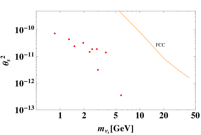
Figure 2: Plots in terms of $m_{\nu_{s}}$ and $\theta_{s}$ in case of NH, where all the constraints discussed above are satisfied. The upper region bounded by the orange line is the favored region of detecting the sterile neutrino by FCC.

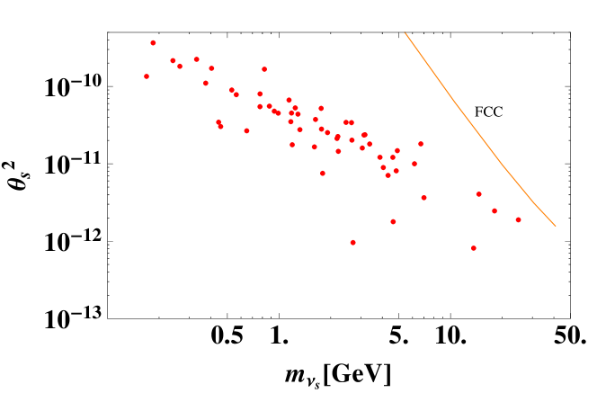
Figure 3: Plots in terms of $m_{\nu_{s}}$ and $\theta_{s}$ in case of IH, where all the constraints discussed above are satisfied. The upper region bounded by the orange line is the favored region of detecting the sterile neutrino by FCC.

V Conclusions and discussions

We have proposed a model with two neutrinophilic Higgs doublet fields $\Phi_{1,2}$, and the vacuum expectation value of the second Higgs doublet is only induced at one-loop level. As a result, the active neutrino masses can be naturally generated to be very small via the tiny VEV $v_{2}$. We have also discussed various phenomenology or constraints from neutrino oscillation data, lepton-flavor violations, the oblique parameters and the muon $g-2$, and the possibilities of collider signatures. In addition, we have pointed out a possibility of sterile neutrino of mass $O(0.1-10)$ GeV from the tiny VEV $v_{2}$. Finally, we have shown a plot of $m_{\nu_{s}}$ and $\theta^{2}_{s}$ that satisfy all the experimental bounds such as neutrino oscillation data, LFVs, and the oblique parameters. We have found an allowed region with $m_{\nu_{s}}\approx 20-50$ GeV and $\theta_{s}^{2}\approx 10^{-12}\sim 10^{-11}$ that is covered by the proposal of the future FCC in pursuing the sterile neutrinos. It is one of the main results that our testability with the FCC experiment is more verifiable than the case of typical canonical seesaw model. This is the direct consequence of our huge matrix of the neutral fermions: $20\times 20$. For the muon $g-2$ we have obtained negative contributions that seem to be against the experimental fact. We may be able to detect a signature by looking at the decay of $\varphi_{R}$ or by the Drell-Yan process of $E^{\prime+}E^{\prime-}$ at the LHC.

At the end of the discussion, it is worthwhile to mention a new possibility of detecting the Goldstone boson $G$. According to a recent work Addazi:2017oge , $G$ can be directly tested by the first order phase transitions in the early Universe triggered by discovery of gravitational waves at the experiment of LIGO Caprini:2015zlo . All of the valid terms to explain it are involved in our theory, our $G$ can also be tested near future.

Appendix A Feynman Integrals

Definitions of $F\left(n,\alpha,\{A_{i};n\}\right)$ is the followings:

$$F(n,\alpha,\{A_{i};n\})\equiv\begin{cases}\int_{0}^{1}\prod_{i=1}^{n}dx_{i}\delta(1-\sum_{i=1}^{n}x_{i})\frac{1}{\left(\sum_{i=1}^{n}x_{i}A_{i}\right)^{\alpha}}.&(\alpha>0)\\ \int_{0}^{1}\prod_{i=1}^{n}dx_{i}\delta(1-\sum_{i=1}^{n}x_{i})\log\left(\sum_{i=1}^{n}x_{i}A_{i}\right).&(\alpha=0)\\ \int_{0}^{1}\prod_{i=1}^{n}dx_{i}\delta(1-\sum_{i=1}^{n}x_{i})\left(\sum_{i=1}^{n}x_{i}A_{i}\right)^{-\alpha}\left(\log\left(\sum_{i=1}^{n}x_{i}A_{i}\right)-\sum_{i=1}^{-\alpha}\frac{1}{i}\right).&(\alpha<0)\end{cases}$$

Where $\{A_{i};n\}=\{A_{1},A_{2},\cdots,A_{n}\}$. The functions have following recurrence relations:

$$F(n,\alpha,\{A_{i};n\}) = \frac{C_{\alpha}}{(A_{n-1}-A_{n})}$$

$$\times\left(F(n-1,\alpha-1,\{A_{i};n-2,A_{n-1}\})-F(n-1,\alpha-1,\{A_{i};n-2,A_{n}\})\right),$$

where $\{A_{i};n-2,B\}=\{A_{1},A_{2},\cdots,A_{n-2},B\}$ and

$$C_{\alpha}=\begin{cases}\frac{1}{1-\alpha}.&(\alpha\neq 1)\\ 1.&(\alpha=1)\end{cases}$$

We can obtain the formula of $F\left(n,\alpha,\{A_{i};n\}\right)$ using the recurrence relations and following relations:

$$F(1,\alpha,\{A;1\})=\begin{cases}\frac{1}{A^{\alpha}}.&(\alpha>0)\\ \log\left(A\right).&(\alpha=0)\\ A^{-\alpha}\left(\log A-\sum_{i=1}^{-\alpha}\frac{1}{i}\right).&(\alpha<0)\end{cases}$$

References

- (1) J. F. Gunion, H. E. Haber, G. L. Kane and S. Dawson, “The Higgs Hunter’s Guide,” Front. Phys. 80, 1 (2000).
- (2) S. Kanemura, T. Matsui and H. Sugiyama, Phys. Lett. B 727, 151 (2013) [arXiv:1305.4521 [hep-ph]].
- (3) T. Nomura and H. Okada, arXiv:1704.03382 [hep-ph].
- (4) W. Wang and Z. L. Han, Phys. Rev. D 94, no. 5, 053015 (2016) doi:10.1103/PhysRevD.94.053015 [arXiv:1605.00239 [hep-ph]].
- (5) S. Kanemura and H. Sugiyama, Phys. Rev. D 86, 073006 (2012) doi:10.1103/PhysRevD.86.073006 [arXiv:1202.5231 [hep-ph]].
- (6) H. Okada and Y. Orikasa, Phys. Rev. D 93, no. 1, 013008 (2016) doi:10.1103/PhysRevD.93.013008 [arXiv:1509.04068 [hep-ph]].
- (7) K. Cheung, H. Ishida and H. Okada, arXiv:1609.06231 [hep-ph].
- (8) N. R. Agostinho, G. C. Branco, P. M. F. Pereira, M. N. Rebelo and J. I. Silva-Marcos, arXiv:1711.06229 [hep-ph].
- (9) E. Fernandez-Martinez, J. Hernandez-Garcia and J. Lopez-Pavon, JHEP 1608, 033 (2016) doi:10.1007/JHEP08(2016)033 [arXiv:1605.08774 [hep-ph]].
- (10) D. V. Forero, M. Tortola and J. W. F. Valle, Phys. Rev. D 90, no. 9, 093006 (2014) doi:10.1103/PhysRevD.90.093006 [arXiv:1405.7540 [hep-ph]].
- (11) A. M. Baldini et al. [MEG Collaboration], Eur. Phys. J. C 76, no. 8, 434 (2016) [arXiv:1605.05081 [hep-ex]].
- (12) J. Adam et al. [MEG Collaboration], Phys. Rev. Lett. 110, 201801 (2013) [arXiv:1303.0754 [hep-ex]].
- (13) K. A. Olive et al. [Particle Data Group], Chin. Phys. C 38, 090001 (2014).
- (14) R. Barbieri, L. J. Hall and V. S. Rychkov, Phys. Rev. D 74, 015007 (2006) doi:10.1103/PhysRevD.74.015007 [hep-ph/0603188].
- (15) C. Patrignani et al. [Particle Data Group], Chin. Phys. C 40, no. 10, 100001 (2016). doi:10.1088/1674-1137/40/10/100001
- (16) K. Nishiwaki, H. Okada and Y. Orikasa, Phys. Rev. D 92, no. 9, 093013 (2015) doi:10.1103/PhysRevD.92.093013 [arXiv:1507.02412 [hep-ph]].
- (17) H. Hatanaka, K. Nishiwaki, H. Okada and Y. Orikasa, Nucl. Phys. B 894, 268 (2015) doi:10.1016/j.nuclphysb.2015.03.006 [arXiv:1412.8664 [hep-ph]].
- (18) K. Cheung, W. Y. Keung and T. C. Yuan, Phys. Rev. D 89, no. 1, 015007 (2014) doi:10.1103/PhysRevD.89.015007 [arXiv:1308.4235 [hep-ph]].
- (19) E. K. Akhmedov, Z. G. Berezhiani, R. N. Mohapatra and G. Senjanovic, Phys. Lett. B 299, 90 (1993) doi:10.1016/0370-2693(93)90887-N [hep-ph/9209285].
- (20) S. Weinberg, Phys. Rev. Lett. 110, no. 24, 241301 (2013) doi:10.1103/PhysRevLett.110.241301 [arXiv:1305.1971 [astro-ph.CO]].
- (21) A. Latosinski, K. A. Meissner and H. Nicolai, arXiv:1205.5887 [hep-ph].
- (22) A. Blondel et al. [FCC-ee study Team], Nucl. Part. Phys. Proc. 273-275, 1883 (2016) doi:10.1016/j.nuclphysbps.2015.09.304 [arXiv:1411.5230 [hep-ex]].
- (23) S. Alekhin et al., Rept. Prog. Phys. 79, no. 12, 124201 (2016) doi:10.1088/0034-4885/79/12/124201 [arXiv:1504.04855 [hep-ph]].
- (24) R. W. Rasmussen and W. Winter, Phys. Rev. D 94, no. 7, 073004 (2016) doi:10.1103/PhysRevD.94.073004 [arXiv:1607.07880 [hep-ph]].
- (25) T. Hambye, F.-S. Ling, L. Lopez Honorez and J. Rocher, JHEP 0907, 090 (2009) Erratum: [JHEP 1005, 066 (2010)] doi:10.1007/JHEP05(2010)066, 10.1088/1126-6708/2009/07/090 [arXiv:0903.4010 [hep-ph]].
- (26) A. Addazi and A. Marciano, arXiv:1705.08346 [hep-ph].
- (27) C. Caprini et al., JCAP 1604, no. 04, 001 (2016) doi:10.1088/1475-7516/2016/04/001 [arXiv:1512.06239 [astro-ph.CO]].