Multiple Object Tracking in Unknown Backgrounds
with Labeled Random Finite Sets

Abstract

This paper proposes an on-line multiple object tracking algorithm that can operate in unknown background. In a majority of multiple object tracking applications, model parameters for background processes such as clutter and detection are unknown and vary with time, hence the ability of the algorithm to adaptively learn the these parameters is essential in practice. In this work, we detail how the Generalized Labeled Multi-Bernouli (GLMB) filter, a tractable and provably Bayes optimal multi-object tracker, can be tailored to learn clutter and detection parameters on-the-fly while tracking. Provided that these background model parameters do not fluctuate rapidly compared to the data rate, the proposed algorithm can adapt to the unknown background yielding better tracking performance.

I Introduction

In a multi-object scenario the number of objects and their individual states evolve in time, compounded by false detections, misdetections and measurement origin uncertainty [1, 2, 3, 4]. For example, in the video dataset KITTI-17 from KITTI datasets [5], see Fig. 1, the number of objects varies with time due to objects coming in and out of the scene, and the detector (e.g. background subtraction, foreground modelling [6]) used to convert each image into point measurements, invariably misses objects in the scene as well as generating false measurements or clutter.

Knowledge of parameters for uncertainty sources such as clutter and detection profile are of critical importance in Bayesian multi-object filtering, arguably, more so than the measurement noise model. Most multi-object tracking techniques are built on the assumption that multi-object system model parameters are known a priori, which is generally not the case in practice [1, 2, 3, 4]. Significant mismatches in clutter and detection model parameters inevitably result in erroneous estimates. For the video tracking example in Fig. 1 the clutter rate and detection profile are not known and have to be guessed before a multi-object tracker can be applied. The tracking performance of the Bayes optimal multi-object tracking filter [7, 8], for the guessed clutter rate and ’true’ clutter rate (that varies with time as shown in Fig. 2), demonstrates significant performance degradation.

Figure 1: Frames 16, 48 of the image sequence from [5] and object detections obtained using the detector in [35]. The number of objects varies with time due to objects coming in and out of the scene. Object estimates (marked by blue boxes) using the standard GLMB filter for guessed clutter rate of 60 (left column) and ’true’ clutter rate (right column). Tracking using ’true’ clutter rate accurately estimated several objects that were missed in the frames on the left.

Except for a few applications, the clutter rate and detection profile of the sensor are not available. Usually these parameters are either estimated from training data or manually tuned. However, a major problem in many applications is the time-varying nature of the misdetection and clutter processes, see Fig. 2 for example. Consequently, there is no guarantee that the model parameters chosen from training data will be sufficient for the multi-object filter at subsequent frames. Thus, current multi-object tracking algorithms are far from being a ’plug-and-play’ technology, since their application still requires cumbersome and error-prone user configuration.

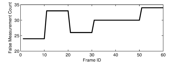
Figure 2: ’True’ clutter rate for the first 60 frames of the dataset[5]. Note that it is not possible to know the true clutter rate for real video data. For illustration we assume that the clutter rate varies slowly and use the average clutter count over a moving 10-frame window as the ’true’ clutter rate.

This paper proposes an online multi-object tracker that learns the clutter and detection model parameters while tracking. Such capability is essential for applications where the clutter rate and detection profile vary with time. Specifically, we detail a GLMB filter for Jump Markov system (JMS), which is applicable to tracking multiple manuevering objects as well as joint tracking and classification of multiple objects. Using the JMS-GLMB filter, we develop a multi-object tracker that can adaptively learn clutter rate and detection profile while tracking, provided that the detection profile and clutter background do not change too rapidly compared to the measurement-update rate. An efficient implementation of the proposed filter and experiments confirm markedly improved performance over existing multi-object filters for unknown background such as the $\lambda$-CPHD filter [9]. Preliminary results have been reported in [10], which outlines a GLMB filter for jump-Markov system model.

We remark that robust Bayesian approaches to problems with model mismatch in the literature such as [11, 12, 13, 14, 15, 16] are too computationally intensive for an on-line multi-object tracker. A Sequential Monte Carlo technique for calibration of time-invariant multi-object model parameters was proposed in [17]. While this approach is quite general it is not directly applicable to time-varying clutter rate and detection profile, and is also too computationally intensive for an on-line tracker. Previous work on CPHD/PHD, multi-Bernoulli and multi-target Bayes filters for unknown clutter rate and detection profile [9], [18, 19, 20, 21, 22, 23] do not output object tracks. Further, the CPHD/PHD, multi-Bernoulli filters require more drastic approximations than the GLMB filter.

The remainder of paper is organized as follows. Section II provides background material on multi-object tracking and the GLMB filter. Section III details two versions of the GLMB filter for a general multi-object JMS model and a non-interacting multi-object JMS model. Section IV presents an efficient implementation of the non-interacting JMS-GLMB filter for tracking in unknown clutter rate and detection profile. Numerical studies are presented in Section V and concluding remarks are given in Section VI.

II Background

This section reviews relevant background on the random finite set (RFS) formulation of multi-object tracking and the GLMB filter. Throughout the article, we adopt the following notations. For a given set $S$, $|S|$ denotes its cardinality (number of elements), $1_{S}(\cdot)$ denotes the indicator function of $S$, and $\mathcal{F}(S)$ denotes the class of finite subsets of $S$. We denote the inner product $\int f(x)g(x)dx$ by $\left\langle f,g\right\rangle$, the list of variables $X_{m},X_{m+1},...,X_{n}$ by $X_{m:n}$, the product $\mathop{\textstyle\prod}_{x\in X}f(x)$ (with $f^{\emptyset}=1$) by $f^{X}$, and a generalization of the Kroneker delta that takes arbitrary arguments such as sets, vectors, integers etc., by

$$\delta_{Y}[X]\triangleq\left\{\begin{array}[]{l}1,\text{ if }X=Y\\ 0,\text{ otherwise}\end{array}\right..$$

II-A Multi-object State

At time $k$, an existing object is described by a vector $x_{k}\in\mathbb{X}$. To distinguish different object trajectories, each object is identified by a unique label $\ell_{k}$ that consists of an ordered pair $(t,i)$, where $t$ is the time of birth and $i$ is the index of individual objects born at time $t$ [7]. The trajectory of an object is given by the sequence of states with the same label.

Formally, the state of an object at time $k$ is a vector $\mathbf{x}_{k}=(x_{k},\ell_{k})\in\mathbb{X\times L}_{k}$, where $\mathbb{L}_{k}$ denotes the label space for objects at time $k$ (including those born prior to $k$). Note that $\mathbb{L}_{k}$ is given by $\mathbb{B}_{k}\cup\mathbb{L}_{k-1}$, where $\mathbb{B}_{k}$ denotes the label space for objects born at time $k$ (and is disjoint from $\mathbb{L}_{k-1}$).

In the RFS approach to multi-object tracking [3, 4]. the collection of object states, referred to as the multi-object state, is naturally represented as a finite set [24]. Suppose that there are $N_{k}$ objects at time $k$, with states $\mathbf{x}_{k,1},...,\mathbf{x}_{k,N_{k}}$, then the multi-object state is defined by the finite set

$$\mathbf{X}_{k}=\{\mathbf{x}_{k,1},...,\mathbf{x}_{k,N_{k}}\}\in\mathcal{F}(\mathbb{X\times L}_{k}),$$

We denote the set $\{\ell:(x,\ell)\in\mathbf{X}\}$ of labels of $\mathbf{X}$ by $\mathcal{L}(\mathbf{X})$. Note that since the label is unique, no two objects have the same label, i.e. $\delta_{|\mathbf{X}|}[|\mathcal{L}(\mathbf{X})|]=1$. Hence $\Delta(\mathbf{X})\triangleq$ $\delta_{|\mathbf{X}|}[|\mathcal{L}_{\mathbf{X}}|]$ is called the distinct label indicator.

A labeled RFS is a random variable on $\mathcal{F}(\mathbb{X}\mathcal{\times}\mathbb{L})$ such that each realization has distinct labels. The distinct label property ensures that at any time no two tracks can share any common points. For the rest of the paper, we follow the convention that single-object states are represented by lower-case letters (e.g. $x$, $\mathbf{x}$), while multi-object states are represented by upper-case letters (e.g. $X$, $\mathbf{X}$), symbols for labeled states and their distributions are bold-faced (e.g. $\mathbf{x}$, $\mathbf{X}$, $\mathbf{\pi}$, etc.), and spaces are represented by blackboard bold (e.g. $\mathbb{X}$, $\mathbb{Z}$, $\mathbb{L}$, etc.). For notational compactness, we drop the time subscript $k$, and use the subscript ‘$+$’ for time $k+1$.

II-B Standard multi-object system model

Given the multi-object state $\mathbf{X}$ at time $k$, each state $(x,\ell)\in\mathbf{X}$ either survives with probability $P_{S}(x,\ell)$ and evolves to a new state $(x_{+},\ell_{+})$ at time $k+1$ with probability density $f_{+}(x_{+}|x,\ell)\delta_{\ell}[\ell_{+}]$ or dies with probability $1-P_{S}(x,\ell)$. The set $\mathbf{B}_{+}$ of new objects born at time $k+1$ is distributed according to the labeled multi-Bernoulli (LMB) density

$$\Delta(\mathbf{B}_{+})\left[1_{\mathbb{B}_{\,+}}\,r_{B,+}\right]^{\mathcal{L(}\mathbf{B}_{+})}\left[1-r_{B,+}\right]^{\mathbb{B}_{+}-\mathcal{L(}\mathbf{B}_{+})}p_{B,+}^{\mathbf{B}_{+}},$$ (1)

where $r_{B,+}(\ell)$ is the probability that a new object with label $\ell$ is born, $p_{B,+}(\cdot,\ell)$ is the distribution of its kinematic state, and $\mathbb{B}_{\,+}$ is the label space of new born objects [7]. The multi-object state $\mathbf{X}_{+}$ (at time $k+1$) is the superposition of surviving objects and new born objects. Note that the label space of all objects at time $k+1$ is the disjoint union $\mathbb{L}_{+}=\mathbb{L}\uplus\mathbb{B}_{+}$. It is assumed that, conditional on $\mathbf{X}$, objects move, appear and die independently of each other.

For a given multi-object state $\mathbf{X}$, each $(x,\ell)\in\mathbf{X}$ is either detected with probability $P_{D}(x,\ell)$ and generates a detection $z\in Z$ with likelihood $g(z|x,\ell)$ or missed with probability $1-P_{D}(x,\ell)$. The multi-object observation is the superposition of the observations from detected objects and Poisson clutter with (positive) intensity $\kappa$. Assuming that, conditional on $\mathbf{X}$, detections are independent of each other and clutter, the multi-object likelihood function is given by [7], [8]

$$g(Z|\mathbf{X})\propto\sum_{\theta\in\Theta}1_{\Theta(\mathcal{L(}\mathbf{X}))}(\theta)\prod\limits_{(x,\ell)\in\mathbf{X}}\psi_{Z_{{}_{\!}}}^{(\theta(\ell))}(x,\ell)$$ (2)

where: $\Theta$ is the set of positive 1-1 maps $\theta:\mathbb{L}\rightarrow\{0$:$|Z|\}$, i.e. maps such that no two distinct arguments are mapped to the same positive value, $\Theta(I)$ is the set of positive 1-1 maps with domain $I$; and

$$\psi_{\!\{z_{1:M}\}\!}^{(j)}(x,\ell)=\left\{\!\!\begin{array}[]{ll}\frac{P_{\!D}(x,\ell)g(z_{j}|x,\ell)}{\kappa(z)},&\!\!\text{if }j=1\text{:}M\\ 1-P_{\!D}(x,\ell),&\!\!\text{if }j=0\end{array}\right.\!\!.$$ (3)

The map $\theta$ specifies which objects generated which detections, i.e. object $\ell$ generates detection $z_{\theta(\ell)}\in Z$, with undetected objects assigned to $0$. The positive 1-1 property means that $\theta$ is 1-1 on $\{\ell:\theta(\ell)>0\}$, the set of labels that are assigned positive values, and ensures that any detection in $Z$ is assigned to at most one object.

For the special case with zero-clutter, i.e. $\kappa$ is identically zero, the multi-object likelihood function still takes the same form, but with $P_{\!D}(x,\ell)g(z_{j}|x,\ell)/\kappa(z)$ replaced by $P_{\!D}(x,\ell)g(z_{j}|x,\ell)$, see [3, 4]. To cover both positive and identically-zero clutter intensities we write

$$\psi_{\!\{z_{1:M}\}\!}^{(j)}(x,\ell)=\left\{\!\!\begin{array}[]{ll}\frac{P_{\!D}(x,\ell)g(z_{j}|x,\ell)}{\kappa(z)+\delta_{0}[\kappa(z)]},&\!\!\text{if }j=1\text{:}M\\ 1-P_{\!D}(x,\ell),&\!\!\text{if }j=0\end{array}\right.\!\!.$$ (4)

II-C Generalized Labeled Multi-Bernoulli

A Generalized Labeled Multi-Bernoulli (GLMB) filtering density, at time $k$, is a multi-object density that can be written in the form

$$\mathbf{\pi}(\mathbf{X})=\Delta(\mathbf{X})\sum_{\xi\in\Xi,I\subseteq\mathbb{L}}\omega^{(I,\xi)}\delta_{I}[\mathcal{L(}\mathbf{X})]\left[p^{(\xi)}\right]^{\mathbf{X}}.$$ (5)

where each $\xi\in\Xi\triangleq\Theta_{0}\times...\times\Theta_{k}$ represents a history of association maps $\xi=(\theta_{1:k})$, each $p^{(\xi)}(\cdot,\ell)$ is a probability density on $\mathbb{X}$, and each $\omega^{(I,\xi)}$ is non-negative with $\sum_{\xi\in\Xi}\sum_{I\subseteq\mathbb{L}}\omega^{(I,\xi)}=1$. The cardinality distribution of a GLMB is given by

$$\Pr(\left|\mathbf{X}\right|\text{=}n)=\sum_{\xi\in\Xi,I\subseteq\mathbb{L}}\delta_{n}\left[\left|I\right|\right]\omega^{(I,\xi)},$$ (6)

while, the existence probability and probability density of track $\ell\in\mathbb{L}$ are respectively

$$r(\ell) =\sum_{\xi\in\Xi,I\subseteq\mathbb{L}}1_{I}(\ell)\omega^{(I,\xi)},$$ (7)

$$p(x,\ell) =\frac{1}{r(\ell)}\sum_{\xi\in\Xi,I\subseteq\mathbb{L}}1_{I}(\ell)\omega^{(I,\xi)}p^{(\xi)}(x,\ell).$$ (8)

Given the GLMB density (5), an intuitive multi-object estimator is the multi-Bernoulli estimator, which first determines the set of labels $L\subseteq$ $\mathbb{L}$ with existence probabilities above a prescribed threshold, and second the mode/mean estimates from the densities $p(\cdot,\ell),\ell\in L$, for the states of the objects. A popular estimator is a suboptimal version of the Marginal Multi-object Estimator [3], which first determines the pair $(L,\xi)$ with the highest weight $\omega^{(L,\xi)}$ such that $\left|L\right|$ coincides with the mode cardinality estimate, and second the mode/mean estimates from $p^{(\xi)}(\cdot,\ell),\ell\in L$, for the states of the objects.

For the standard multi-object system model the GLMB density is a conjugate prior, and is also closed under the Chapman-Kolmogorov equation [7]. Moreover, the GLMB posterior can be tractably computed to any desired accuracy in the sense that, given any $\epsilon>0$, an approximate GLMB within $\epsilon$ from the actual GLMB in $L_{1}$ distance, can be computed (in polynomial time) [8]. The GLMB filtering density can be propagated forward in time via a prediction step and an update step as in[8] or in one single step as in [25]. Since the number of components grow exponentially in the predicted/filtered densities during prediction/update stages, truncation of hypotheses with low weights is essential during implementation. Polynomial complexity schemes for truncation of insignificant weights were given in [8] and [25], via Murty’s algorithm with a quartic (or at best cubic) complexity, or via Gibbs sampling with a linear complexity, where the complexity is given in the number of measurements.

III Jump Markov System GLMB Filtering

We first derive from the GLMB recursion a multi-object filter for Jump Markov system (JMS) in subsection III-A, which is applicable to tracking multiple manuevering objects as well as joint tracking and classification of multiple objects. When the modes of the multi-object JMS do not interact, the JMS-GLMB recursion reduces to a more tractable form, which is presented in subsection III-B. This special case is then used to develop a multi-object tracker that can operate in unknown background in section IV.

III-A GLMB filter for Jump Markov Systems

A Jump Markov System (JMS) consists of a set of parameterised state space models, whose parameters evolve with time according to a finite state Markov chain. A JMS can be specified in terms of the standard system parameters for each mode or class as follows.

Let $\mathbb{M}$ be the (discrete) index set of modes in the system. Suppose that mode $m$ is in effect at time $k$, then the state transition density from $\zeta$, at time $k$, to $\zeta_{+}$, at time $k+1$, is denoted by $f_{+}^{(m)}(\zeta_{+}|\zeta)$, and the likelihood of $\zeta$ generating the measurement $z$ is denoted by $g^{(m)}(z|\zeta)$ [26], [27], [28]. Moreover, the joint transition of the state and mode assumes the form:

$$f_{+}(\zeta_{+},m_{+}|\zeta,m)=f_{+}^{(m_{+})}(\zeta_{+}|\zeta)\vartheta_{+}(m_{+}|m),$$ (9)

where $\vartheta_{+}(m_{+}|m)$ denotes the probability of switching from mode $m$ to $m_{+}$ (and satisfies $\sum_{m_{+}\in\mathbb{M}}\vartheta_{+}(m_{+}|m)=1$). Note that by defining the augmented state as $x=(\zeta,m\mathbf{)}\in\mathbb{X}\times\mathbb{M}$, a JMS model can be expressed as a standard state space model with transition density (9) and measurement likelihood function $g(z|\zeta,m)=g^{(m)}(z|\zeta)$.

In a multi-object system, each object is identified by a label $\ell$ that remains unchanged throughout its life, hence the JMS state equation for such an object is written as

$$\!\!\!\!f_{+}(\zeta_{+},m_{+}|\zeta,m,\ell)\!\!\! = \!\!\!f_{+}^{(m_{+})}(\zeta_{+}|\zeta,\ell)\vartheta_{+}(m_{+}|m)$$ (10)

$$\!\!\!\!g(z|\zeta,m,\ell)\!\!\! = \!\!\!g^{(m)}(z|\zeta,\ell)$$ (11)

Additionally, to emphasize the dependence on the mode, the survival, birth and detection parameters are, respectively, denoted as

$$p_{B,+}^{(m_{+})}(\zeta_{+},\ell_{+}) \triangleq p_{B,+}(\zeta_{+},m_{+},\ell_{+}),$$

$$P_{S}^{(m)}(\zeta,\ell) \triangleq P_{S}(\zeta,m,\ell),$$

$$P_{D}^{(m)}(\zeta,\ell) \triangleq P_{D}(\zeta,m,\ell).$$

Substituting these parameters and the JMS state equations (10)-(11) into the GLMB recursion in [25] yields the so-called JMS-GLMB recursion.

Proposition 1.

If the filtering density at time $k$ is the GLMB (5), then the filtering density at time $k+1$ is the GLMB

$$\mathbf{\pi}_{\!}(\mathbf{X_{+\!}}|Z_{+\!})\!\propto\!\Delta_{\!}(_{\!}\mathbf{X_{\!+}}_{\!})\!\!\!\!\sum\limits_{I\!,\xi,I_{\!+},\theta_{\!+\!}}\!\!\!\!\omega^{(I,\xi)}\omega_{Z_{{}_{\!}+}}^{(_{\!}I_{\!},\xi,I_{\!+\!},\theta_{\!+\!})}\delta_{{}_{\!}I_{+\!}}[\mathcal{L}(_{\!}\mathbf{X_{\!+}}_{\!})]\!\left[p_{Z_{{}_{\!}+_{\!}}}^{(_{\!}\xi,\theta_{\!+\!})}{}_{\!}\right]^{\!\mathbf{X_{\!+}}}\!$$ (12)

where $I\in\mathcal{F}(\mathbb{L})$,$\;\xi\in\Xi$,$\;I_{+}\in\mathcal{F}(\mathbb{L}_{+})$,$\;\theta_{+}\in\Theta_{+}$,

$$\omega_{Z_{{}_{\!}+}}^{(_{\!}I_{\!},\xi,I_{\!+\!},\theta_{\!+\!})}= 1_{{\Theta}_{\!+\!}(I_{+})}(\theta_{\!+\!})\left[1-\bar{P}_{S}^{(\xi)}\right]^{\!I\!-I_{\!+}}\!\left[\bar{P}_{S\!}^{(\xi)}\right]^{\!I\cap I_{+\!}}\times$$

$$\left[1-r_{B\!,+}\right]^{\mathbb{B}_{\!+\!}-I_{\!+}\!}\;r_{B\!,+}^{\mathbb{B}_{\!{+}}\cap I_{+\!}}\!\left[\bar{\psi}_{{}_{\!}Z_{{}_{\!}+}}^{(_{\!}\xi,\theta_{{}_{\!}+\!})}\right]^{I_{+}}$$ (13)

$$\bar{P}_{S\!}^{(\xi)}(\ell)= \sum_{m\in\mathbb{M}}\bar{P}_{S\!}^{(\xi)}(m,\ell),$$ (14)

$$\bar{P}_{S\!}^{(\xi)}(m,\ell)= \left\langle p^{(\xi)\!}(\cdot,m,\ell),P_{S}^{(m)}(\cdot,\ell)\right\rangle,$$ (15)

$$\bar{\psi}_{{}_{\!}Z_{{}_{\!}+}}^{(\xi,\theta_{+\!})}(\ell)= \sum_{m_{+}\in\mathbb{M}}\bar{\psi}_{{}_{\!}Z_{{}_{\!}+}}^{(\xi,\theta_{+\!})}(m_{+},\ell),$$ (16)

$$\bar{\psi}_{{}_{\!}Z_{{}_{\!}+}}^{(\xi,\theta_{+\!})}(m_{+},\ell)= \left\langle\bar{p}_{+}^{(\xi)}(\cdot,m_{+},\ell_{{}_{\!}}),\psi_{{}_{\!}Z_{{}_{\!}+}\!}^{(\theta_{{}_{\!}+}(\ell))}(\cdot,m_{+},\ell_{{}_{\!}})\right\rangle$$ (17)

$$\!\bar{p}_{+}^{(\xi)\!}(\zeta_{+},m_{+},\ell)=1_{\mathbb{B}_{+}}\!(\ell)p_{B}^{(m_{+})}(\zeta_{+},\ell)\;+\text{ \ \ \ \ \ \ \ \ \ \ \ \ \ \ \ \ \ \ \ \ \ \ }$$

$$1_{\mathbb{L}}(\ell)\frac{\sum\limits_{m\in\mathbb{M}}{\tiny\!}\!\left\langle\!{\small P}_{S}^{(m)}{\small(\cdot,\ell)f}_{+}^{(m_{+})}{\small(\zeta}_{+}{\small|\cdot,\ell),p}^{(\xi)}{\small(\cdot,m,\ell)}\!\right\rangle\!{\small\vartheta(m}_{+}{\small|m)}}{{\small\bar{P}}_{S}^{(\xi)}{\small(\ell)}}$$ (18)

$$p_{Z_{{}_{\!}+}}^{(\xi_{\!},\theta_{\!+\!})\!}(\zeta_{+},m_{+},\ell)= \frac{\bar{p}_{+}^{(\xi)\!}(\zeta_{+},m_{+},\ell)\psi_{Z_{+}}^{(\theta_{{}_{\!}+\!}(\ell))\!}(\zeta_{+},m_{+},\ell)}{\bar{\psi}_{Z_{+}}^{(\xi,\theta_{{}_{\!}+})}(m_{+},\ell_{{}_{\!}})}$$ (19)

$$\psi_{\!\{z_{1:|Z|}\}\!}^{(j)}(\zeta,m,\ell)= \left\{\!\!\begin{array}[]{ll}\!\frac{P_{D}^{(m)}(\zeta,\ell)g^{(m)}(z_{j\!}|_{{}_{\!}}\zeta,\ell)}{\kappa(z_{j})+\delta_{0}[\kappa(z_{j})]},&\!\!\!\text{if }j\in\left\{1,...,|Z|\right\}\\ \!1-P_{D}^{(m)}(\zeta,\ell),&\!\!\!\text{if }j=0\end{array}\right.\!\!$$ (22)

Notice that the above expression is in $\delta$-GLMB form since it can be written as a sum over $I_{\!+},\xi,\theta_{+}$ with weights

$$\omega_{Z_{+}}^{(I_{+},\xi,\theta_{+})}\propto\sum\limits_{I}\omega^{(I,\xi)}\omega_{Z_{+}}^{(I,\xi,I_{+},\theta_{+})}.$$

This special case of the GLMB recursion is particularly useful for tracking multiple manuevering objects and joint multi-object tracking and classification. Indeed the application of the JMS-GLMB recursion to multiple manuevering object tracking has been reported our preliminary work [10], where separate prediction and update steps was introduced. The same result was independently reported in [29].

III-B Multi-Class GLMB

The JMS-GLMB recursion can be applied to the joint multi-object tracking and classification problem by using the mode as the class label (not to be confused to object label). What distinguishes this problem from generic JMS-GLMB filtering is that the modes do not interact with each other in the following sense:

1. All possible states of a new object with the same object label share a common mode (class label);

2. An object cannot switch between different modes from one time step to the next.

Let $\mathbb{B}^{(m)}$ denote the set of labels of all elements in $\mathbb{X\times M}\times\mathbb{B}$ with mode $m$. Then condition 1 implies that the label sets $\mathbb{B}^{(m)}$ and $\mathbb{B}^{(m^{\prime})}$ for different modes $m$ and $m^{\prime}$ are disjoint (otherwise there exist a label $\ell$ in both $\mathbb{B}^{(m)}$ and $\mathbb{B}^{(m^{\prime})}$, which means there are states in $\mathbb{X\times M}\times\mathbb{B}$ with different modes $m$ and $m^{\prime}$ but share a common label $\ell$). Furthermore, the sets $\mathbb{B}^{(m)}$, $m\in\mathbb{M}$ cover $\mathbb{B}$, i.e. $\mathbb{B}=\bigcup_{m\in\mathbb{M}}\mathbb{B}^{(m)}$, and thus form a partition of the space $\mathbb{B}$. A new object is classified as class $m$ (and has mode $m$) if and only if its label falls into $\mathbb{B}^{(m)}$. Thus for an LMB birth model, condition 1 means

$$r_{B,+}(\ell_{+}) = \sum_{m_{+}\in\mathbb{M}}r_{B,+}^{(m_{+})}1_{\mathbf{\mathbb{B}}_{+}^{(m_{+})}}(\ell_{+}),$$ (23)

$$p_{B,+}^{(m_{+})}(\zeta_{+},\ell_{+}) = p_{B,+}^{(m_{+})}(\zeta_{+})1_{\mathbf{\mathbb{B}}_{+}^{(m_{+})}}(\ell_{+}).$$ (24)

Note that $r_{B,+}^{(m_{+})}$ and $p_{B,+}^{(m_{+})}(\zeta_{+})$ are respectively the existence probability and probability density of the kinematics $\zeta_{+}$ of a new object given mode $m_{+}$, while $1_{\mathbf{\mathbb{B}}_{+}^{(m_{+})}}(\ell_{+})$ is the probability of mode $m_{+}$ given label $\ell_{+}$.

Condition 2 means that the mode transition probability

$$\vartheta(m_{+}|m)=\delta_{m}[m_{+}],$$ (25)

which implies that each object belongs to exactly one of the classes in $\mathbb{M}$ for its entire life. Consequently, the non-interacting mode condition means that at time $k$, the label space for all class $m$ objects is $\mathbb{L}^{(m)}=\biguplus\nolimits_{t=0}^{k}\mathbb{B}_{t}^{(m)}$, and the set of all possible labels is given by the disjoint union $\mathbb{L}=\biguplus\nolimits_{m\in\mathbb{M}}\mathbb{L}^{(m)}$.

For a multi-object JMS system with non-interacting modes, the JMS-GLMB recursion reduces to a form where the weights and multi-object exponentials can be separated according to classes. We call this form the multi-class GLMB.

Proposition 2.

Let $\mathbf{X}_{\!\!}^{(m)}$ denote the subset of $\mathbf{X}$ with mode $m$, and hence $\mathbf{X}=\biguplus\nolimits_{m\in\mathbb{M}}\mathbf{X}^{(m)}$. Suppose that the hybrid multi-object density at time $k$ is a GLMB of the form

$$\mathbf{\pi}(\mathbf{X})=\sum_{\xi,I}1_{{\Theta}(I)}(\xi\perp{\Theta})\prod\limits_{m\in\mathbb{M}}\mathbf{\pi}^{(I^{(m)},\xi^{(m)})}(\mathbf{X}_{\!\!}^{(m)})$$ (26)

where $\xi\in\Xi$, $I\subseteq\mathbb{L}$, $\xi\perp{\Theta}$ denotes the projection $\xi$ into the space ${\Theta}$, $I^{(m)}\triangleq I\cap\mathbb{L}^{(m)}$, $\xi^{(m)}=\xi|_{\mathbb{L}_{0}^{(m)}\times...\times\mathbb{L}_{k}^{(m)}}$ (i.e. the map $\xi$ restricted to $\mathbb{L}_{0}^{(m)}\times...\times\mathbb{L}_{k}^{(m)}$), and

$$\mathbf{\pi}^{(I,\xi)}(\mathbf{X})\triangleq\Delta(\mathbf{X})w^{(I,\xi)}\delta_{{}_{\!}I}[\mathcal{L}(\mathbf{X}_{\!})]\left[p^{(\xi)}\right]^{\mathbf{X}}$$ (27)

Then the hybrid multi-object filtering density at time $k+1$ is the GLMB

$$\mathbf{\pi}_{\!Z_{+}\!}(\mathbf{X_{+}})\!\propto\!\!\!\!\sum_{\xi,I,_{\!}\theta_{\!+\!},I_{+\!}}\!\!\!\!1_{{\Theta}_{\!+\!}(I_{+\!})}(\theta_{\!+\!})\!\!\!\prod\limits_{m\in\mathbb{M}}\!\!\mathbf{\pi}_{Z_{+}\!}^{\!(m,I_{\!}^{(m)},\xi^{(m)},I_{\!+\!}^{(m)},\theta_{\!+\!}^{\!(m)})\!}(\mathbf{X}_{+\!}^{(m)\!})$$ (28)

where $I_{\!+\!}\in\!\mathcal{F}(\mathbb{L}_{\!+})$,$\;\theta_{\!+\!}\in\!\Theta_{+}$, $I_{\!+}^{(m)}=I_{\!+}\!\cap\!\mathbb{L}_{+}^{(m)}$, $\theta_{+}^{(m)}=\theta_{+}|_{\mathbb{L}_{+}^{(m)}}$

$$\!\!\!\!\!\!\!\!\!\!\!\!\!\!\!\!\!\!\!\!\!\!\!\mathbf{\pi}_{Z_{+}\!}^{(m,I_{\!},\xi,I_{\!+\!},\theta_{\!+\!})}(\mathbf{X}_{+\!})=$$

$$\!\!\!\!\Delta_{\!}(\mathbf{X}_{+})w_{Z_{{}_{\!}+}}^{(m,I_{\!},\xi,I_{\!+\!},\theta_{\!+\!})}w^{(I,\xi)}\delta_{{}_{\!}I_{+}}[\mathcal{L}(\mathbf{X}_{+\!})]\left[p_{Z_{{}_{\!}+_{\!}}}^{(_{\!}\xi,\theta_{\!+\!})}{}_{\!}\right]^{\mathbf{X}_{+}}$$ (29)

$$w_{Z_{{}_{\!}+}}^{(_{\!}m,I_{\!},\xi,I_{\!+\!},\theta_{\!+\!})} =\left[\bar{\psi}_{{}_{\!}Z_{{}_{\!}+}}^{(_{\!}\xi,\theta_{{}_{\!}+\!})}(m,\cdot)\right]^{I_{+}}\left[1-r_{B\!,+}\right]^{\mathbb{B}_{\!+\!}^{(m)}-I_{\!+}\!}r_{B\!,+}^{\mathbb{B}_{\!{+}}^{(m)}\cap I_{+\!}}$$

$$\times\left[1-\bar{P}_{S}^{(\xi)}(m,\cdot)\right]^{\!I\!-I_{\!+}}\!\left[\bar{P}_{S\!}^{(\xi)}(m,\cdot)\right]^{\!I\cap I_{+\!}}$$ (30)

$$\bar{P}_{S}^{(\xi)}(m,\ell) =\left\langle p^{(\xi)\!}(\cdot,m,\ell),P_{S}^{(m)}(\cdot,\ell)\right\rangle,$$ (31)

$$\bar{\psi}_{{}_{\!}Z_{{}_{\!}+}}^{(\xi,\theta_{+\!})}(m,\ell) =\left\langle\bar{p}_{+}^{(\xi)}(\cdot,m,\ell_{{}_{\!}}),\psi_{{}_{\!}Z_{{}_{\!}+}\!}^{(\theta_{{}_{\!}+}(\ell))}(\cdot,m,\ell_{{}_{\!}})\right\rangle,$$ (32)

$$\bar{p}_{+}^{(\xi)_{\!}}(\zeta,m,\ell)= 1_{\mathbb{L}_{\!}^{(m)}}(\ell)\frac{\!\left\langle P_{S}^{(m)}(\cdot,\ell)f_{+}^{(m)}(\zeta|\cdot,\ell)),p^{(\xi)}(\cdot,m,\ell)\right\rangle}{\bar{P}_{S}^{(\xi)}(m,\ell)}$$

$$+ 1_{\mathbb{B}_{+}^{(m)}}\!(\ell)p_{B}^{(m)}(\zeta,\ell)$$ (33)

$$p_{Z_{{}_{\!}+}}^{(\xi_{\!},\theta_{\!+\!})\!}(\zeta,m,\ell) =\frac{\bar{p}_{+}^{(\xi)}(\zeta,m,\ell)\psi_{Z_{+}}^{(\theta_{{}_{\!}+}(\ell))}(\zeta,m,\ell)}{\bar{\psi}_{Z_{+}}^{(\xi,\theta_{{}_{\!}+})}(m,\ell)}$$ (34)

$$\psi_{\!\{z_{1:|Z|}\}\!}^{(j)}(\zeta,m,\ell)=\Big{\{}\begin{array}[]{ll}\!\frac{P_{D}^{(m)}(\zeta,\ell)g^{(m)}(z_{j\!}|_{{}_{\!}}\zeta,\ell)}{\kappa(z_{j})+\delta_{0}[\kappa(z_{j})]},\!\text{if }j\in\left\{1,...,|Z|\right\}&\\ \!1-P_{D}^{(m)}(\zeta,\ell),\;\;\;\;\;\;\text{if }j=0&\end{array}$$ (35)

Proof.

Note that the $\mathbb{L}_{0}^{(m)}\times...\times\mathbb{L}_{k}^{(m)},m\in\mathbb{M}$ form a partition of $\mathbb{L}_{0}\times...\times\mathbb{L}_{k}$ , and since each $\xi^{(m)}$ was defined as a restrictions of $\xi$ over $\mathbb{L}_{0}^{(m)}\times...\times\mathbb{L}_{k}^{(m)}$, $\xi$ is completely characterized by the $\xi^{(m)},m\in\mathbb{M}$. By defining

$$\omega^{(I,\xi)} = 1_{{\Theta}(I)}(\xi\perp{\Theta})\prod\limits_{m\in\mathbb{M}}w^{(I^{(m)},\xi^{(m)})}$$ (36)

$$p^{(\xi)}(\zeta,m,\ell) = \left[p^{(\xi^{(m)})}(\zeta,m,\ell)\right]^{1_{\mathbb{L}^{(m)}}(\ell)}$$ (37)

it can be seen that (26) is a GLMB of the form (5) since

$$\delta_{{}_{\!}I}[\mathcal{L}(\mathbf{X}_{\!})] = \prod\limits_{m\in\mathbb{M}}\delta_{{}_{\!}I^{(m)}}[\mathcal{L}(\mathbf{X}_{\!}^{(m)})]$$

$$\left[p^{(\xi)}\right]^{\mathbf{X}} = \left[p^{(\xi)}\right]^{\biguplus\nolimits_{m\in\mathbb{M}}\mathbf{X}^{(m)}}=\prod\limits_{m\in\mathbb{M}}\left[p^{(\xi^{(m)})}{}_{\!}\right]^{\mathbf{X}^{(m)}}.$$

Thus by applying Proposition 1, the hybrid multi-object filtering density at time $k+1$ is given by (12-22). Substituting (36), (37), (23-25) into (12-22), decomposing

$$\mathbf{X}_{+} = \biguplus\nolimits_{m\in\mathbb{M}}\mathbf{X}_{+}^{(m)}$$ (38)

$$\omega_{Z_{{}_{\!}+}}^{(_{\!}I_{\!},\xi,I_{\!+\!},\theta_{\!+\!})} = 1_{{\Theta}_{\!+\!}(I_{+})}(\theta_{\!+\!})\prod\limits_{m\in\mathbb{M}}w_{Z_{{}_{\!}+}}^{(m,I_{\!}^{(m)},\xi^{(m)},I_{\!+\!}^{(m)},\theta_{\!+\!}^{(m)})}$$ (39)

$$p_{Z_{{}_{\!}+_{\!}}}^{(_{\!}\xi,\theta_{\!+\!})}{} = \left(p_{Z_{{}_{\!}+_{\!}}}^{(_{\!}\xi^{(m)},\theta_{\!+\!}^{(m)})}{}_{\!}\right)^{1_{\mathbb{L}_{+}^{(m)}}(\ell)}$$ (40)

and rearranging yields (28). Note that (25) ensures that $m_{+}=m$.    

Given a GLMB filtering density of the multi-class form (26), the GLMB filtering density for class $c\in\mathbb{M}$, can be obtained by marginalizing the other classes according to the following proposition.

Proposition 3.

For the multi-class GLMB (26), the marginal GLMB for class $c$ is given by

$$\mathbf{\pi}\left(\mathbf{X}^{(c)}\right)=\Delta(\mathbf{X}^{(c)})\sum_{\xi,I}\omega^{(I,\xi)}\delta_{{}_{\!}I^{(c)}}[\mathcal{L}(\mathbf{X}_{\!}^{(c)})]\left[p^{(\xi^{(c)})}\right]^{\mathbf{X}^{(c)}}$$

Proof.

Note that

$$\!\!\!\!\!\!\!\!\!\!\!\!\!\!\int\mathbf{\pi}^{(I^{(m)},\xi^{(m)})}(\mathbf{X}_{\!\!}^{(m)})\delta\mathbf{X}^{(m)}$$

$$= \!\int\!\Delta(\mathbf{X}^{(m)\!})w^{(I^{(m)\!},\xi^{(m)})}\delta_{{}_{\!}I^{(m)\!}}[\mathcal{L}(\mathbf{X}_{\!}^{(m)})]\!\left[p^{(\xi)}\right]^{\!\mathbf{X}^{\!(m)}}\!\delta\mathbf{X}^{(m)}$$

$$= \!w^{(I^{(m)},\xi^{(m)})}.$$

Since, the $\mathbf{X}^{(m)}$, $m\in\mathbb{M}$ are disjoint,

$$\mathbf{\pi}(\mathbf{X}^{(c)})\!\! = \!\!\int\mathbf{\pi}\left(\mathop{\textstyle\biguplus}\limits_{m\in\mathbb{M}}\mathbf{X}^{(m)}\right)\delta\left(\mathop{\textstyle\biguplus}\limits_{m\in\mathbb{M}-\{c\}}\mathbf{X}^{(m)}\right)$$

$$= \!\!\int\sum_{\xi,I}\!1_{{\Theta}(I)}(\xi\!\perp\!{\Theta})\times$$

$$\!\!\prod\limits_{m\in\mathbb{M}}\mathbf{\pi}^{(I^{(m)},\xi^{(m)})}(\mathbf{X}_{\!\!}^{(m)})\delta\left(\mathop{\textstyle\biguplus}\limits_{m\in\mathbb{M}-\{c\}}\mathbf{X}^{(m)}\right)$$

$$= \!\!\sum_{\xi,I}\!1_{{\Theta}(I)}(\xi\!\perp\!{\Theta})\mathbf{\pi}^{(I^{(c)},\xi^{(c)})}(\mathbf{X}_{\!\!}^{(c)})\times$$

$$\!\!\prod\limits_{m\in\mathbb{M}-\{c\}}\int\mathbf{\pi}^{(I^{(m)},\xi^{(m)})}(\mathbf{X}_{\!\!}^{(m)})\delta\mathbf{X}^{(m)}$$

$$= \!\!\sum_{\xi,I}\!1_{{\Theta}(I)}(\xi\!\perp\!{\Theta})\mathbf{\pi}^{(I^{(c)},\xi^{(c)})}(\mathbf{X}_{\!\!}^{(c)})\times$$

$$\!\!\prod\limits_{m\in\mathbb{M}-\{c\}}\!\!\!\!w^{(I^{(m)},\xi^{(m)})}.$$

$$= \!\!\Delta(\mathbf{X}^{(c)})\sum_{\xi,I}\omega^{(I,\xi)}\delta_{{}_{\!}I^{(c)}}[\mathcal{L}(\mathbf{X}_{\!}^{(c)})]\left[p^{(\xi^{(c)})}\right]^{\mathbf{X}^{(c)}}.$$

   

IV GLMB Filtering with Unknown Background

Clutter or false detections are generally understood as detections that do not correspond to any object [1, 2, 3, 4]. Since the number false detections and their values are random, clutter is usually modelled by RFSs in the literature [30, 3, 4]. The simplest and the most commonly used clutter model is the Poisson RFS [30], in most cases, with a uniform intensity over the surveillance region. Alternatively clutter can be treated as detections originating from clutter generators–objects that are not of interest to the tracker [9], [18, 19, 20].

In [9] a CPHD recursion was derived to propagate separate intensity functions for clutter generators and objects of interest, and their collective cardinality distribution of the hybrid multi-object state. Similarly, in [20] analogous multi-Bernoulli recursions were derived to propagate the disjoint union of objects of interest and clutter generators. In this work we show that the multi-class GLMB filter is an effective multi-object object tracker that can operate under unknown background by learning the clutter and detection model on-the-fly.

This section details an on-line multi-object tracker that operates in unknown clutter rate and detection profile. In particular we propose a GLMB clutter model in subsection IV-A by treating clutter as a special class of objects with completely uncertain dynamics, and describe a dedicated GLMB recursion for propagating the joint filtering density of clutter generators and objects of interest. Implementation details are given in subsection IV-B. Extension of the proposed algorithm to accommodate unknown detection profile is described in subsection IV-F.

IV-A GLMB Joint Object-Clutter Model

We propose to model the finite set of clutter generators and objects of interest as two non-interacting classes of objects, and propagate this so-called hybrid multi-object filtering density forward in time via the multi-class GLMB recursion. The GLMB filtering density of the hybrid multi-object state captures all relevant statistical information on the objects of interest as well as the clutter generators. What distinguishes the objects of interest from clutter generators is that the former have relatively predictable dynamics whereas the latter have completely random dynamics.

In the hybrid multi-object model, the Poisson clutter intensity $\kappa$ is identically 0 and each detection is generated from either a clutter generator or an object of interest, which constitute, respectively, the two modes (or classes) 0 and 1 of the mode space $\mathbb{M}=\{0,1\}$. Since the classes are non-interacting, there are no switchings between objects of interest and clutter generators. Moreover, the label space for new born clutter generators $\mathbf{\mathbb{B}}^{(0)}$ and the label space for new born objects of interest $\mathbf{\mathbb{B}}^{(1)}$ are disjoint and the LMB birth parameters are given by

$$r_{B,+}(\ell_{+}) = r_{B,+}^{(0)}1_{\mathbf{\mathbb{B}}_{+}^{(0)}}(\ell_{+})+r_{B,+}^{(1)}1_{\mathbf{\mathbb{B}}_{+}^{(1)}}(\ell_{+}),$$

$$p_{B,+}^{(m_{+})}(\zeta_{+},\ell_{+}) = p_{B,+}^{(m_{+})}(\zeta_{+})1_{\mathbf{\mathbb{B}}_{+}^{(m_{+})}}(\ell_{+})$$

Since clutter are distinguishable from targets by their completely random dynamics, each clutter generator has a transition density independent of the previous state and a uniform measurememt likelihood in the observation region with volume $V$

$$f_{+}^{(0)}(\zeta_{+}|\zeta,\ell) = s(\zeta_{+})$$

$$g^{(0)}(z|\zeta,\ell) = u(z)V^{-1}$$

Note that the labels of clutter generators can effectively be ignored since it is implicit that their labels are distinct but are otherwise uninformative. Further, for Gaussian implementations it is assumed that the survival and detection probabilities for clutter generators are state independent

$$P_{S}^{(0)}(\zeta,\ell) = P_{S}^{(0)}$$

$$P_{D}^{(0)}(\zeta,\ell) = P_{D}^{(0)}$$

Applying the multi-class GLMB recursion to this model, it can be easily seen that all clutter generators are functionally identical (from birth through prediction and update)

$$p_{B}^{(0)}(\zeta,\ell)=\bar{p}_{+}^{(\xi^{(0)})}(\zeta,0,\ell)=p_{Z_{+}}^{(\xi^{(0)},\theta_{+}^{(0)})}(\zeta,0,\ell)=s(\zeta)$$

and that the weight update for clutter generators reduces to

$$\!\!\!\!\!\!w_{Z_{{}_{\!}+}}^{(0,_{\!}I_{\!}^{(0)},\xi^{(0)},I_{\!+\!}^{(0)},\theta_{\!+\!}^{(0)})}$$

$$= \left[1-P_{S}^{(0)}\right]^{|I^{(0)}-I_{+}^{(0)}|}\left[P_{S}^{(0)}\right]^{|I^{(0)}\cap I_{+}^{(0)}|}\times$$

$$\left[1-r_{B,+}^{(0)}\right]^{|\mathbb{B}_{+}^{(0)}-I_{+}^{(0)}|}\left[r_{B,+}^{(0)}\right]^{|\mathbb{B}_{{+}}^{(0)}\cap I_{+}^{(0)}|}\times$$

$$\left[1-P_{D,+}^{(0)}\right]^{|\{\ell\in I_{+}^{(0)}:\theta_{+}^{(0)}(\ell)=0\}|}\left[P_{D,+}^{(0)}V^{-1}\right]^{|\{\ell\in I_{+}^{(0)}:\theta_{+}^{(0)}(\ell)>0\}|}$$ (41)

Thus propagation of clutter generators within each GLMB component reduces to propagation of their weights

$$w_{Z_{+}}^{(0,I_{+}^{(0)},\xi^{(0)},\theta_{+}^{(0)})}=\mathop{\textstyle\sum}\nolimits_{I^{(0)}}w^{(I^{(0)},\xi^{(0)})}w_{Z_{+}}^{(0,I^{(0)},\xi^{(0)},I_{+}^{(0)},\theta_{+}^{(0)})}.$$

IV-B Implementation

The key challenge in the implemention of the multi-class GLMB filter is the propagation of the GLMB components, which involves, for each parent GLMB component $(I,\xi)$, searching the space $\mathcal{F}(\mathbb{L}_{\!+})\times\Theta_{+}$ to find a set of $(I_{\!+},\theta_{\!+\!})$ such that the children components $(I_{\!},\xi,I_{\!+\!},\theta_{\!+\!})$ have significant weights $\omega_{Z_{{}_{\!}+}}^{(_{\!}I_{\!},\xi,I_{\!+\!},\theta_{\!+\!})}$. In [25], the set of $(I_{\!+},\theta_{\!+\!})$ is generated from a Gibbs sampler with stationary distribution is constructed so that only valid children components have positive probabilities, and those with high weights are more likely to be sampled than those with low weights. A direct application of this approach to generate new children would, however, be expensive, for the following reasons.

Let $P=|I|$, $P^{(0)}=|I^{(0)}|$, $P^{(1)}=|I^{(1)}|$ and $M=|Z_{+}|$. According to [25] the complexity of the joint prediction and update via Gibbs sampling with $T$ iterations is $\mathcal{O}(TP^{2}M)$. Since the present formulation treat clutter as objects, the total number of hypothesized objects $P\geq P^{(0)}\geq M$, and hence the complexity is at least $\mathcal{O}(TM^{3})$, which is cubic in the number of measurements and results in a relatively inefficient implementation. This occurs because the majority of the computational effort is spent on clutter generators even though they are not of interest. This problem is exacerbated as the clutter rate increases.

In the following we propose a more efficient implementation by focusing on the filtering density of the objects of interest instead of the hybrid multi-object filtering density. Observe that given any $(I_{+}^{(1)},\theta_{\!+\!}^{(1)})\in\mathcal{F}(\mathbb{L}_{\!+}^{(1)})\times\Theta_{+}^{(1)}$, and $(I_{+}^{(0)},\theta_{\!+\!}^{(0)})\in\mathcal{F}(\mathbb{L}_{\!+}^{(0)})\times\Theta_{+}^{(0)}$, where $\Theta_{+}^{(m)}$ denotes the space of positive 1-1 maps from $\mathbb{L}_{+}^{(m)}$ to $\{0,1,...,M\}$, we can uniquely define

$$(I_{\!+},\theta_{\!+\!})\triangleq(I_{+}^{(1)}\uplus I_{+}^{(0)},1_{\mathbb{L}_{\!+}^{(1)}}\theta_{\!+\!}^{(1)}+1_{\mathbb{L}_{\!+}^{(0)}}\theta_{\!+\!}^{(0)}).$$ (42)

Further, the weight of the resulting component $(I_{\!},\xi,I_{\!+\!},\theta_{\!+\!})$ is

$$\omega_{Z_{{}_{\!}+}}^{(_{\!}I_{\!},\xi,I_{\!+\!},\theta_{\!+\!})}=1_{{\Theta}(I_{\!+\!})}(\theta_{\!+\!})w_{Z_{+}\!}^{\!(0,I_{\!}^{(0)},\xi^{(0)},I_{\!+\!}^{(0)},\theta_{\!+\!}^{\!(0)})\!}w_{Z_{+}\!}^{\!(1,I_{\!}^{(1)},\xi^{(1)},I_{\!+\!}^{(1)},\theta_{\!+\!}^{\!(1)})\!}$$ (43)

see Proposition 2 (39). Note that if $\theta_{\!+\!}$ is not a valid association map then $1_{{\Theta}(I_{\!+\!})}(\theta_{\!+\!})=0$, and hence the weight is zero.

For each parent GLMB component $(I,\xi)$, rather than searching for $(I_{\!+},\theta_{\!+\!})$ with significant $\omega_{Z_{{}_{\!}+}}^{(_{\!}I_{\!},\xi,I_{\!+\!},\theta_{\!+\!})}$ in the space $\mathcal{F}(\mathbb{L}_{\!+})\times\Theta_{+}$, we:

1. seek $(I_{+}^{(1)},\theta_{\!+\!}^{(1)})$ with significant $w_{Z_{{}_{\!}+}}^{(_{\!}1,I_{\!}^{(1)},\xi^{(1)},I_{\!+\!}^{(1)},\theta_{\!+\!}^{(1)})}$ from the smaller space $\mathcal{F}(\mathbb{L}_{\!+}^{(1)})\times\Theta_{+}^{(1)}$;

2. for each such $(I_{+}^{(1)},\theta_{\!+\!}^{(1)})$ find the $(I_{+}^{(0)},\theta_{\!+\!}^{(0)})$ with the best $w_{Z_{{}_{\!}+}}^{(_{\!}0,I_{\!}^{(0)},\xi^{(0)},I_{\!+\!}^{(0)},\theta_{\!+\!}^{(0)})}$, subject to the constraint

   $$1_{\mathbb{L}_{\!+}^{(1)}}\theta_{\!+\!}^{(1)}+1_{\mathbb{L}_{\!+}^{(0)}}\theta_{\!+\!}^{(0)}\in{\Theta}(I_{+}^{(1)}\uplus I_{+}^{(0)});$$ (44)

3. construct $(I_{\!+},\theta_{\!+\!})$ from $(I_{+}^{(1)},\theta_{\!+\!}^{(1)})$ and $(I_{+}^{(0)},\theta_{\!+\!}^{(0)})$ via (42) and compute the corresponding weight via (43).

Due to the constraint 44, $1_{{\Theta}(I_{\!+\!})}(\theta_{\!+\!})=1$, and hence, it follows from (43) that the resulting GLMB component $(I_{\!},\xi,I_{\!+\!},\theta_{\!+\!})$ also has significant weight.

The advantage of this strategy is two fold:

• searching over a much smaller space $\mathcal{F}(\mathbb{L}_{\!+}^{(1)})\times\Theta_{+}^{(1)}$ results in a linear complexity in the measurements $\mathcal{O}(T(P^{(1)})^{2}M)$ since typically $P^{(1)}<<M$;

• finding $(I_{+}^{(0)},\theta_{\!+\!}^{(0)})$ with the best weight subject to the constraint $\theta_{\!+\!}\in{\Theta}(I_{\!+\!})$ is straight forward and requires miminal computation.

IV-C Propagating Objects of Interest

One way to generate significant $(I_{+}^{(1)},\theta_{\!+\!}^{(1)})$ is to design a Gibbs sampler with stationary distribution $w_{Z_{{}_{\!}+}}^{(_{\!}1,I_{\!}^{(1)},\xi^{(1)},I_{\!+\!}^{(1)},\theta_{\!+\!}^{(1)})}$. However, this approach requires computing the hybrid multi-object density, which we try to avoid in the first place.

A much more efficient alternative is to treat the multi-Bernoulli clutter as Poisson with matching intensity, and apply the standard GLMB filter (the JMS-GLMB filter (12) with a single-mode), where the Gibbs sampler [31] (or Murty’s algorithm [32]) can be used to obtain significant $(I_{+}^{(1)},\theta_{\!+\!}^{(1)})$ [25]. Since there are $|I^{(0)}|$ clutter generators from the previous time with survival probability $P_{S}^{(0)}$, and $|\mathbf{\mathbb{B}}_{+}^{(0)}|$ clutter birth with probability $r_{B,+}^{(0)}$, the predicted clutter intensity is given by $\hat{\kappa}_{+}=(P_{S}^{(0)}|I^{(0)}|+r_{B,+}^{(0)}|\mathbf{\mathbb{B}}_{+}^{(0)}|)P_{D,+}^{(0)}V^{-1}$. Note that a Poisson RFS has larger variance on the number of clutter points than a multi-Bernoulli with matching intensity. Hence, in treating clutter as a Poisson RFS, we are effectively tempering with the clutter model to induce the Gibbs sampler (or Murty’s algorithm) to generate more diverse components [25].

Following [25], let us enumerate $Z_{+}=\{z_{1:M}\}$, $I^{(1)}=\{\ell_{1:R}\}$, and $\mathbb{B}_{+}^{(1)}=\{\ell_{R+1:P}\}$. The $(I_{\!+}^{(1)},\theta_{\!+\!}^{(1)})\in$ $\mathcal{F}(\mathbb{L}_{+}^{(1)})\times\Theta(I_{+}^{(1)})$ at time $k+1$ with significant weights are determined by solving a ranked assignment problem with cost matrix $[\eta_{i}^{(\xi^{(1)})}(j)]$, $i=1:P$,$~{}j=-1:M$, where

$$\eta_{i}^{(\xi^{(1)})\!}(j)\!=\!\left\{\!\!\begin{array}[]{ll}1-\bar{P}_{S\!}^{(\xi^{(1)})}(1,\ell_{i})&\!\!\ell_{i}\in I^{(1)},~{}j<0\\ \bar{P}_{S}^{(\xi^{(1)})}(1,\ell_{i})\bar{\psi}_{Z_{+}}^{(\xi^{(1)},\theta_{+}^{(1)})\!}(1,\ell_{i})&\!\!\ell_{i}\in I^{(1)},~{}j\geq 0\\ 1-r_{B,+}(\ell_{i})&\!\!\ell_{i}\in\mathbb{B}_{+}^{(1)},~{}j<0\\ r_{B,+}(\ell_{i})\bar{\psi}_{Z_{+}}^{(\xi^{(1)},\theta_{+}^{(1)})\!}(1,\ell_{i})&\!\!\ell_{i}\in\mathbb{B}_{+}^{(1)},~{}j\geq 0\end{array}\right.$$

$$\bar{\psi}_{Z_{+}}^{(\xi^{(1)},\theta_{+}^{(1)})}(1,\ell)\!\! = \!\!\left\langle\bar{p}_{+}^{(\xi^{(1)})}(\cdot,1,\ell),\psi_{Z_{+}}^{(\theta_{+}^{(1)}(\ell))}(\cdot,1,\ell)\right\rangle$$

$$\psi_{Z_{+}}^{(j)}(\zeta,1,\ell)\!\! = \!\!\left\{\!\begin{array}[]{ll}\frac{P_{D,+}^{(1)}(\zeta,\ell)g_{+}^{(1)}(z_{j}|\zeta,\ell)\!}{\hat{\kappa}_{+}},&\!\!\text{if }j\in\left\{1,...,M\right\}\\ 1-P_{D,+}^{(1)}(\zeta,\ell),&\!\!\text{if }j=0\end{array}\right.$$

Such a ranked assignment problem can be solved by Murty’s algorithm or the Gibbs sampler given in Section III-D [25].

IV-D Propagating Clutter Generators

Given $(I_{\!+}^{(1)},\theta_{\!+\!}^{(1)})$ pertaining to the objects of interest, we proceed to determine $(I_{\!+}^{(0)},\theta_{\!+\!}^{(0)})$ pertaining to clutter generators, which maximizes $\omega_{Z_{{}_{\!}+}}^{(_{\!}0,I_{\!}^{(0)},\xi^{(0)},I_{\!+\!}^{(0)},\theta_{\!+\!}^{(0)})}$ where $I_{\!+\!}^{(0)}\subseteq$ ${}_{\!}I_{\!}^{(0)}\cup\mathbb{B}_{+}^{(0)}$ and $\theta_{\!+\!}^{(0)}:I_{\!+\!}^{(0)}\rightarrow\{0:M\}$ subject to constraint (44).

Denote by $Z_{+}^{(1)}\subseteq Z_{+}$ the set of measurements assigned to $I_{\!+}^{(1)}$ by $\theta_{\!+\!}^{(1)}$ and the remaining set of measurements $Z_{+}-$ $Z_{+}^{(1)}$, due to clutter generators, by $Z_{+}^{(0)}$. Recall that clutter generators are functionally identical except in label and that their propagation reduces to calculating their corresponding weights (41). Let $N_{S}^{(0)}=|I^{(0)}\cap I_{+}^{(0)}|$ and $N_{B,+}^{(0)}=|\mathbb{B}_{{+}}^{(0)}\cap I_{+}^{(0)}|$ denote the counts of surviving and new born clutter generators respectively. Then $|I^{(0)}-I_{+}^{(0)}|=|I^{(0)}|-N_{S}^{(0)}$ and $|\mathbb{B}_{+}^{(0)}-I_{+}^{(0)}|=|\mathbb{B}_{+}^{(0)}|-N_{B,+}^{(0)}$. Observe that the count $|Z_{+}^{(0)}|$ of clutter must equal the number of detections of clutter generators according to $(I_{\!+}^{(0)},\theta_{\!+\!}^{(0)})$, i.e. $|Z_{+}^{(0)}|=|\{\ell\in I_{+}^{(0)}:\theta_{+}^{(0)}(\ell)>0\}|$ and hence the count of misdetections of clutter generators according to $(I_{\!+}^{(0)},\theta_{\!+\!}^{(0)})$ is $N_{S}^{(0)}+N_{B,+}^{(0)}-|Z_{+}^{(0)}|=|\{\ell\in I_{+}^{(0)}:\theta_{+}^{(0)}(\ell)=0\}|$. Consequently the weight (41) can be rewritten as

$$\!\!\!\!\!\!\!\!\omega_{Z_{{}_{\!}+}}^{(0,I_{\!}^{(0)},\xi^{(0)},I_{\!+\!}^{(0)},\theta_{\!+\!}^{(0)})}\!$$

$$= \left[1-P_{S}^{(0)\!}\right]^{\!|I^{(0)\!}|-N_{S}^{(0)}}\!\!\!\left[P_{S}^{(0)\!}\right]^{\!N_{S}^{(0)}}\!\!\!\left[1-r_{B,+\!}^{(0)}\right]^{\!|\mathbb{B}_{+}^{(0)}|-N_{B,+}^{(0)}}\times$$

$$\left[r_{B,+\!}^{(0)}\right]^{\!N_{B,+}^{(0)}}\left[1-P_{D,+}^{(0)\!}\right]^{\!N_{S}^{(0)}+N_{B,+}^{(0)}-|Z_{+}^{(0)\!}|}\!\left[P_{D,+}^{(0)\!}V^{-1}\right]^{\!|Z_{+}^{(0)}|}$$

$$\propto \left[\!\frac{P_{S}^{(0)}(1-P_{D,+}^{(0)})}{1-P_{S}^{(0)}}\!\right]^{\!N_{S}^{(0)}}\!\left[\!\frac{r_{B,+}^{(0)}(1-P_{D,+}^{(0)})}{1-r_{B,+}^{(0)}}\!\right]^{\!N_{B,+}^{(0)}}$$

Thus seeking the best $(I_{\!+}^{(0)},\theta_{\!+\!}^{(0)})$ subject to constraint (44) reduces to seeking the best $(N_{S}^{(0)},N_{B,+}^{(0)})$ subject to the constraints $0\leq N_{S}^{(0)}\leq$ $|I^{(0)}|$, $0\leq N_{B,+}^{(0)}\leq$ $|\mathbb{B}_{+}^{(0)}|$ and $N_{S}^{(0)}+N_{B,+}^{(0)}\leq|Z_{+}^{(0)}|$.

IV-E Linear Gaussian Update Parameters

Let $\mathcal{N}(\cdot;\bar{\zeta},P)$ denotes a Gaussian density with mean $\bar{\zeta}$ and covariance $P$. Then for a linear Gaussian multi-object model of the objects of interest $P_{S}^{(1)}(\zeta,\ell)=P_{S}^{(1)}$, $P_{D}^{(1)}(\zeta,\ell)=P_{D}^{(1)}$, $f_{+}^{(1)}(\zeta_{+}|\zeta,\ell)=\mathcal{N}(\zeta_{+};F\zeta,Q)$, $g^{(1)}(z|\zeta,\ell)=\mathcal{N}(z;H\zeta,R)$, and $p_{B,+}^{(1)}(\zeta_{+})=\mathcal{N}(\zeta_{+};\bar{\zeta}_{+}^{(1)},P_{+}^{(1)})$, where $F$ is the transition matrix, $Q$ is the process noise covariance, $H$ is the observation matrix, $R$ is the observation noise covariance, $\bar{\zeta}_{+}^{(1)}$ and $P_{+}^{(1)}$ are the mean and covariance of the kinematic state of a new object of interest. If each current density of an object of interest is a Gaussian of the form

$$p^{(\xi^{(1)})_{\!}}(\zeta,1,\ell)=\mathcal{N}(\zeta;\bar{\zeta}^{(\xi^{(1)})}(\ell),P^{(\xi^{(1)})}(\ell))$$ (46)

then the terms (32), (33), (34) can be computed analytically using the following identities:

$$\int\mathcal{N}(\zeta;\bar{\zeta},P)\mathcal{N}(\zeta_{+};F\zeta,Q)d\zeta=\mathcal{N}(\zeta_{+};F\bar{\zeta},FPF^{T}+Q),$$

$$\!\!\!\!\!\!\!\!\!\!\!\!\!\!\!\!\!\!\!\!\!\!\!\!\!\!\!\!\!\!\mathcal{N}(\zeta;\bar{\zeta},P)\mathcal{N}(z;H\zeta,R)$$

$$= q(z)\mathcal{N}(\zeta;\bar{\zeta}+K(z-H\bar{\zeta}),[I-KH]P),$$

$$q(z) = \mathcal{N}(z;H\bar{\zeta},HPH^{T}+R),$$

$$K = PH^{T}\left[HPH^{T}+R\right]^{-1}.$$

IV-F Extension to Unknown Detection Probability

Following the approach in [9], to jointly estimate an unknown detection probability, we augment a variable $a\in[0,1]$ to the state, i.e. $\mathbf{x}=(\zeta,m,a,\ell)$, so that

$$P_{D}^{(m)}(\zeta,a,\ell)=a.$$ (47)

Additionally, in this model $g^{(m)}(z|\zeta,a,\ell)=g^{(m)}(z|\zeta,\ell)$, $P_{S}^{(m)}(\zeta,a,\ell)=P_{S}^{(m)}$, $p_{B,+}^{(1)}(\zeta_{+},a_{+})=p_{B,+}^{(1)}(\zeta_{+})p_{B,+}^{(1)}(a_{+})$, and the transition density is given by

$$f_{+}^{(m)}(\zeta_{+},a_{+}|\zeta,a,\ell)=f_{+}^{(m)}(\zeta_{+},|\zeta,\ell)f_{+}^{(\Delta)}(a_{+}|a).$$ (48)

The unknown detection probability is then modelled on a Beta distribution $\beta(\cdot,s,t)$ where $s$ and $t$ are positive shape parameters and the single-object state density is modelled by a Beta-Gaussian density:

$$\!\!\!\!\!\!\!p^{(\xi^{(1)})_{\!}}(\zeta,1,a,\ell)$$

$$= \beta(a;s^{(\xi^{(1)})}(\ell),t^{(\xi^{(1)})}(\ell))\mathcal{N}(\zeta;m^{(\xi^{(1)})}(\ell),P^{(\xi^{(1)})}(\ell)$$

Note that in practice, we only use the Beta model for the unknown detection probability of the objects of interest. For clutter generators, we use a fixed detection probability between 0.5 and 1. Values close to 0.5 result in a large variance on the clutter cardinality and faster reponse to changes in clutter parameter, while the converse is true for values close to 1.

Analytic computation of the terms (32), (33), (34) can be performed separately for the Gaussian part (which has been given in the previous subsection) and the Beta part using [9]:

$$\beta(a_{+};s_{+},t_{+})=\int\beta(a;s,t)f_{+}^{(\Delta)}(a_{+}|a)da$$

where

$$s_{+} = \left(\frac{\mu_{\beta}(1-\mu_{\beta})}{\sigma_{\beta}^{2}}-1\right)\mu_{\beta},$$

$$t_{+} = \left(\frac{\mu_{\beta}(1-\mu_{\beta})}{\sigma_{\beta}^{2}}-1\right)\left(1-\mu_{\beta}\right).$$

$$\mu_{\beta} = \frac{s}{s+t}\;,\;\;\;\;\;\sigma_{\beta}^{2}=\frac{st}{(s+t)^{2}(s+t+1)}$$

(note that $\beta(\cdot;s_{+},t_{+})$ has the same mean $\mu_{\beta}$ as $\beta(\cdot;s,t)$ but a larger variance than $\sigma_{\beta}$) and

$$(1-a)\beta(a;s,t) = \frac{B(s,t+1)}{B(s,t)}\beta(a;s,t+1),$$

$$a\beta(a;s,t) = \frac{B(s+1,t)}{B(s,t)}\beta(a;s+1,t),$$

where $B(s,t)=\mathop{\textstyle\int}\nolimits_{0}^{1}a^{s-1}(1-a)^{t-1}da$.

V Numerical Studies

V-A Simulations

The following simulation scenario is used to test the proposed robust multi-object filter. The target state vector $[x,y,\dot{x},\dot{y}]^{T}$ consists of cartesian coordinates and the velocities. Objects of interest move according to a constant velocity model, with zero-mean Gaussian process noise of covariance

$$Q_{f}={v_{f}}^{2}\begin{bmatrix}T^{4}/4&T^{3}/2&0&0\\ T^{3}/2&T^{2}&0&0\\ 0&0&T^{4}/4&T^{3}/2\\ 0&0&T^{3}/2&T^{2}\end{bmatrix}$$

where $v_{f}=5ms^{-1}$ and $T=1s$. Objects of interest are born from a labeled multi Bernoulli distribution with four components of 0.03 birth probability, and birth densities

$$\mathcal{N}(\cdotp,[0,0,0,0]^{T},P_{\gamma}),$$

$$\mathcal{N}(\cdotp,[400,-600,0,0]^{T},P_{\gamma}),$$

$$\mathcal{N}(\cdotp,[-800,-200,0,0]^{T},P_{\gamma}),$$

$$\mathcal{N}(\cdotp,[-200,800,0,0]^{T},P_{\gamma}),$$

where $P_{\gamma}=\operatorname{diag}([50,50,50,50]).$ The probability of survival is set at 0.99.

Objects of interest enter and leave the observation region $[-1000,1000]m\times[-1000,1000]m$ at different times reaching a maximum of ten targets. The measurements are the object positions obtained through a sensor located at coordinate $(0,0)$. Measurement noise is assumed to be distributed Gaussian with zero-mean and covariance $Q_{r}$ where $v_{r}=3ms^{-1}$.

$$Q_{r}={v_{r}}^{2}\begin{bmatrix}1&0\\ 0&1\end{bmatrix}$$

The detection model parameters for all new born objects of interest are set at $s=9$ and $t=1$ resulting in a mean of 0.9 for the detection probability. At the initial timestep, clutter generators are born from a (labeled) multi-Bernoulli distribution with 120 components, each with 0.5 birth probability and uniform birth density. At subsequent timesteps clutter generators are born from a (labeled) multi-Bernoulli distribution with 30 components, each with 0.5 birth probability and uniform birth density. Probability of survival and probability of detection of the clutter generators are both set at 0.9.

Four scenarios corresponding to four different pairings of average (unknown) clutter rate and detection probability (see Table 1) are studied.

Scenario ID	Clutter Rate	Detection Probability
1	10	0.97
2	10	0.85
3	70	0.97
4	varying between 25-35	0.95

TABLE I: Simulation Parameters unknown to the filter

The Fig. 3(a) shows the OSPA[33] errors obtained from 100 Monte Carlo runs (OSPA c = 300, p = 1) for the proposed GLMB filter in comparison with $\lambda$-CPHD[9] filter for scenario 1. Estimated clutter rates and detection probabilites by the two filters are shown in Fig. 3(b), while estimated tracks for objects of interest taken from a single run is shown in Fig. 3(c). It can be seen that for the given parameters, the GLMB filter performs far better than the $\lambda$-CPHD in terms of clutter rate, detection probability and track estimation for objects of interest.

We further investigate the performance of the proposed algorithm by varying the background parameters in scenarios 2 and 3. The average detection probability in scenario 2 is lower than that of scenario 1, while the average clutter rate in scenario 3 is higher than that of scenario 1. Note from Figure 3 that $\lambda$-CPHD filter begins to fail in scenario 1. The OSPA errors for 100 Monte Carlo runs, estimates of the clutter rate and detection probabilities for the more challenging scenarios 2 and 3 are given in Fig. 4, Fig. 5 at which $\lambda$-CPHD competely breaks down. On the other hand the proposed GLMB filter is capable of accurately tracking the objects of interest as well as estimating the unknown clutter and detection parameters. The fourth scenario comprises of a wavering clutter rate with comparison to the $\lambda$-CPHD filter. Perceiving Fig. 6 it is clear that that the proposed filter outperforms $\lambda$-CPHD and is quite adept at converging swiftly to the shifted clutter rate.

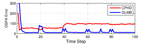
(a) OSPA Error

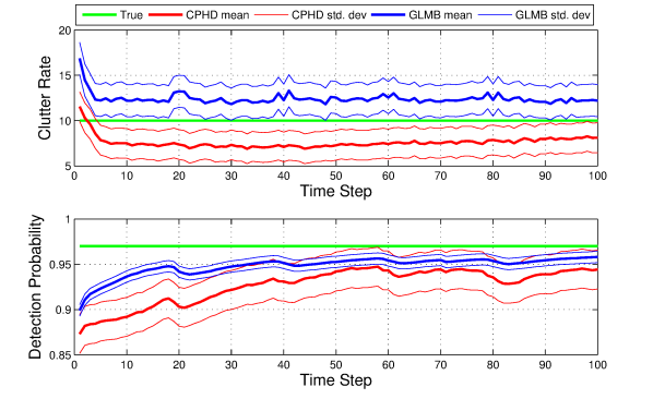
(b) estimated clutter and detection parameters

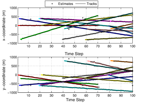
(c) Track Estimations

Figure 3: Scenario 1. The bumps in the OSPA error for GLMB in 3(a) appear close to time steps where a new birth or a death of an object of interest occurs.

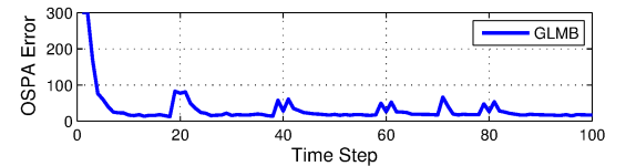
(a) OSPA Error

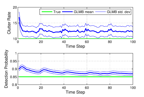
(b) estimated clutter and detection parameters

Figure 4: Scenario 2. Comparison with $\lambda$-CPHD not included as it completely fails at this juncture.

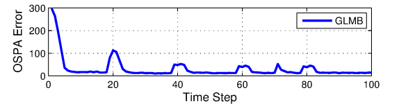
(a) OSPA Error

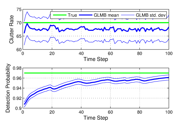
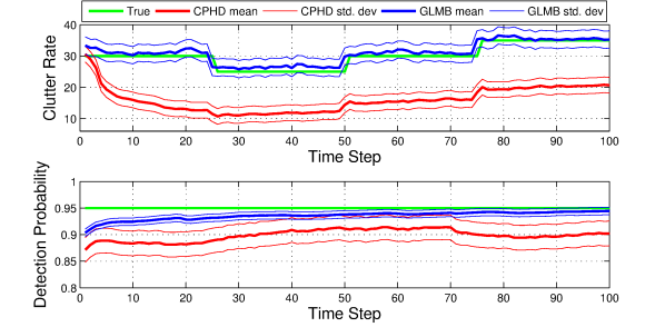
(b) estimated clutter and detection parameters

Figure 5: Scenario 3. Comparison with $\lambda$-CPHD not included as it completely fails at this juncture.

(a) OSPA Error

(b) estimated clutter and detection parameters

Figure 6: Scenario 4.

V-B Video Data

The proposed filter for jointly unknown clutter rate and detection probability is tested on two image sequences: S2.L1 from PETS2009 datasets [34] and KITTI-17 from KITTI datasets [5]. The detections are obtained using the detection algorithm in [35].

Dataset 1: The state vector consists of the target $x,y$ positions and the velocities in each direction. The process noise is assumed to be distributed from a zero-mean Gaussian with covariance $Q_{f}$ where $v_{f}=2$ pixels. Actual targets are assumed to be born from a labeled multi Bernoulli distribution with seven components of 0.03 birth probability, and Gaussian birth densities,

$$\!\!\!\!\!\!\mathcal{N}(\cdotp,[260;260;0;0]^{T},P_{\gamma}),\mathcal{N}(\cdotp,[740;370;0;0]^{T},P_{\gamma}),$$

$$\!\!\!\!\!\!\mathcal{N}(\cdotp,[10;200;0;0]^{T},P_{\gamma}),\mathcal{N}(\cdotp,[280;80;0;0]^{T},P_{\gamma}),$$

$$\!\!\!\!\!\!\mathcal{N}(\cdotp,[750;130;0;0]^{T},P_{\gamma}),\mathcal{N}(\cdotp,[650;270;0;0]^{T},P_{\gamma}),$$

$$\!\!\!\!\!\!\mathcal{N}(\cdotp,[500;200;0;0]^{T},P_{\gamma}),\text{ where }P_{\gamma}=\operatorname{diag}([10;10;3;3]).$$

The observation space is a $756\times 560$ pixel image frame. Actual target measurements contain the $x,y$ positions with measurement noise assumed to be distributed zero-mean Gaussian with covariance $Q_{r}$ with $v_{r}=3$ pixels. Clutter targets are born from a multi Bernoulli distribution with 30 birth components in the firstmost time step and 12 components in subsequent time steps each with 0.5 birth probability and uniform birth density. Probability of survival and detection for clutter targets are both set at 0.9.

The Fig. 7 shows tracking results at frames 20, 40 and 100 respectively. True and estimated clutter cardinality statistics are given in Fig. 8. From these figures it can be observed that the filter successfully outputs object tracks and that the estimated clutter rate nearly overlays the true clutter rate.

Dataset 2: The detection results from this dataset (KITTI17) comprises of a higher number of false measurements than the PETS2009 S2.L1 dataset. The state vector consists of the target $x,y$ positions and the velocities in each direction. The process noise is assumed to be distributed from a zero-mean Gaussian with covariance $Q_{f}$ where $v_{f}=2$ pixels. Actual targets are assumed to be born from a labeled multi Bernoulli distribution with three components of 0.05 birth probability, and birth densities

$$\!\!\!\!\!\!\mathcal{N}(\cdotp,[550;200;0;0]^{T},P_{\gamma}),\mathcal{N}(\cdotp,[1200;250;0;0]^{T},P_{\gamma}),$$

$$\!\!\!\!\!\!\mathcal{N}(\cdotp,[500;250;0;0]^{T},P_{\gamma})\text{where }P_{\gamma}=\operatorname{diag}([10;10;1;1]).$$

State transition function for actual targets are based on constant velocity model with a 0.99 probability of survival. Process noise is assumed to be distributed from a zero-mean Gaussian with covariance $Q_{f}$ with $v_{f}=2$ pixels per frame. The observation space is a 1220$\times$350 pixel image frame. Actual target measurements contain the $x,y$ positions with measurement noise assumed to be distributed zero-mean Gaussian with covariance $Q_{r}$ with $v_{r}=3$ pixels. Clutter target are born from 60 identical and uniformly distributed birth regions in the firstmost time step and 20 birth regions in the subsequent time steps each with a birth probability of 0.5. Probability of survival and detection for clutter targets are both set at 0.9.

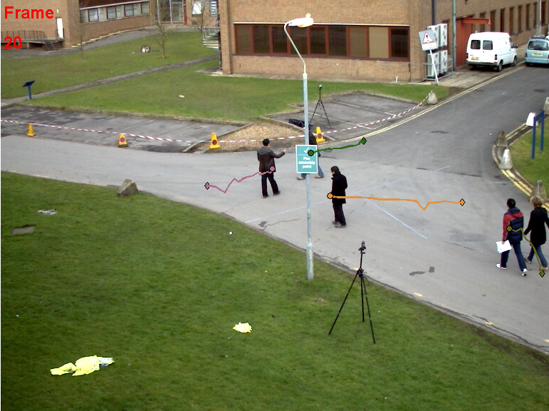
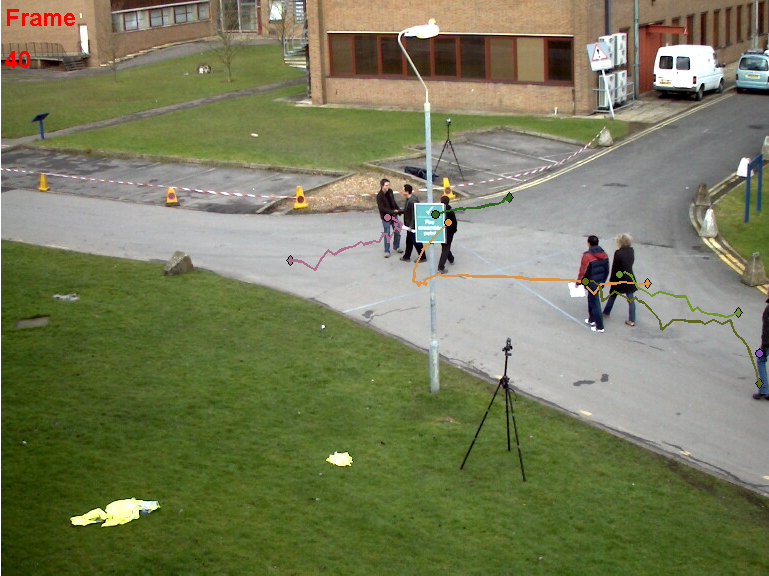
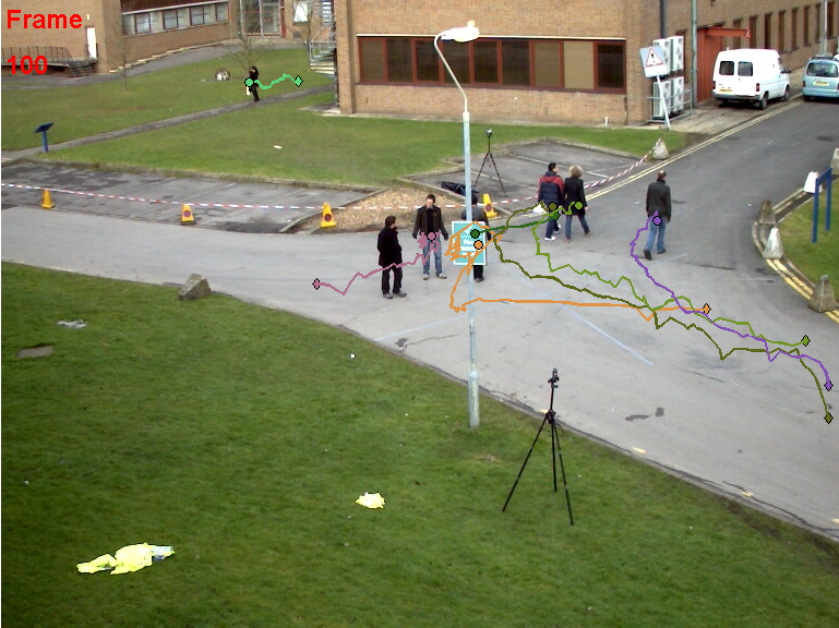
Figure 7: Tracking results for frames 20, 40, 100 in dataset 1.

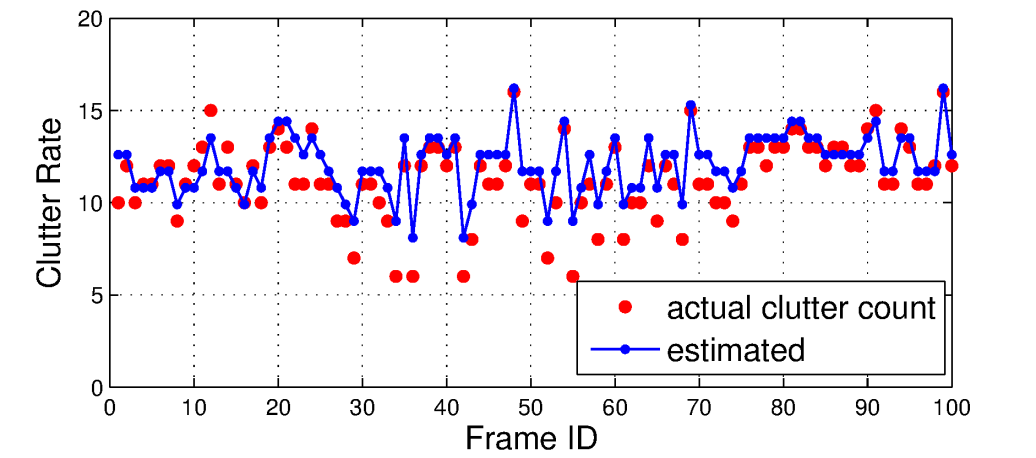
Figure 8: Estimated clutter rate for dataset 1.

The frames on the left of Fig. 9 shows tracking results for frames 15, 35 and 50 obtained from the standard GLMB filter for the guessed clutter rate of 60. The frames on the right of Fig. 9 shows tracking results for the same frames using the proposed filter. When comparing each frame pair it can be noted that some objects that were missed by the standard algorithm with the guessed clutter rate has been picked up by the proposed algorithm. Comparison between true and estimated clutter cardinality statistics given in Fig. 10 demonstrates that the estimated clutter rate is close enough to the true clutter rate to achieve a similar performance if fed back to the standard algorithm[8].

Figure 9: Tracking results for frames 15,35,50 with guessed clutter rate 60 (left) and the proposed filter (right) for dataset 2.

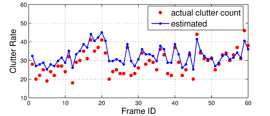
Figure 10: Estimated clutter rate for dataset 2.

VI Conclusion

In this paper we have proposed a tractable algorithm for tracking multiple objects in environments with unknown model parameters, such as clutter rate and detection probability, based on the GLMB filter. Specifically, objects of interest and clutter objects are treated as non-interacting classes of objects, and a GLMB recursion for propagating the joint filtering density of these classes are derived, along with an efficient implementation. Simulations and applications to video data demonstrate that the proposed filter has good tracking performance in the presence of unknown background and outperforms the $\lambda$-CPHD filter. Moreover, it can also estimate the clutter rate and detection probability parameters while tracking.

References

• [1] Y. Bar-Shalom and T. E. Fortmann, Tracking and Data Association.   San Diego: Academic Press, 1988.
• [2] S. S. Blackman and R. Popoli, Design and Analysis of Modern Tracking Systems, ser. Artech House radar library.   Artech House, 1999.
• [3] R. Mahler, Statistical Multisource-Multitarget Information Fusion.   Artech House, 2007.
• [4] R. Mahler, Advances in Statistical Multisource-Multitarget Information Fusion,    Artech House, 2014.
• [5] A. Geiger, P. Lenz, and R. Urtasun, “Are we ready for Autonomous Driving? The KITTI Vision Benchmark Suite,” Proc. 19th  Conference on Computer Vision and Pattern Recognition, 2012.
• [6] A. Elgammal, R. Duraiswami, D. Harwood, and L.S. Davis, “Background and foreground modeling using nonparametric kernel density estimation for visual surveillance,” Proceedings of the IEEE, vol. 90, no. 7, pp. 1151-1163, 2002.
• [7] B.-T. Vo and B.-N. Vo, “Labeled random finite sets and multi-object conjugate priors,” IEEE Trans. Signal Process., vol. 61, no. 13, pp. 3460–3475, 2013.
• [8] B.-N. Vo, B.-T. Vo, and D. Phung, “Labeled random finite sets and the Bayes multi-target tracking filter,” IEEE Trans. Signal Process., vol. 62, no. 24, pp. 6554–6567, 2014.
• [9] R. Mahler, B.-T. Vo, and B.-N. Vo “CPHD filtering with unknown clutter rate and detection profile,” IEEE Trans. Signal Processing, vol. 59, no. 8, pp. 3497-3513, 2011.
• [10] Y. Punchihewa, B.-N. Vo, and B.-T. Vo, “A Generalized Labeled Multi-Bernoulli Filter for Maneuvering Targets,” Proc. 19th  Int. Conf. Inf. Fusion, pp. 980-986. July 2016. Available: https://arxiv.org/pdf/1603.04565.pdf
• [11] F. G. Cozman, ”A brief introduction to the theory of sets of probability measures”, Tech Rep. is CMU-RI-TR 97-24, Robotics Insititute, Carnegie Mellon Universities, 1999.
• [12] B. Noack, V. Klumpp, D. Brunn and U. Hanebeck, ”Nonlinear Bayesian estimation with convex sets of probability densities”, FUSION 2008, Cologne.
• [13] P. Walley, Statistical Reasonning with Imprecise Probabilities, Monographs on Statistics and Applied Probability, Vol. 42, London Chapman and Hall, 1991.
• [14] S. Basu, ”Ranges of posterior probabilities over a distribution band”, Journal of Statistical Planning and Inference, Vol. 44, pp. 149-166, 1995.
• [15] J. Berger, D. Insua, F. Ruggeri, ”Robust Bayesian Analysis”, Lecture notes in Statistics, Vol. 152, pp. 1-32, Springer, 2000.
• [16] M. Berliner, ”Hierachical Bayesian time series models”, in Maximum Entropy and Bayesian Methods, K. Hauson and R. Silver Eds, Kluwer, 1996, pp. 15-22.
• [17] S. Singh, N. Whiteley, and S. Godsil, ”An approximate likelihood method for estimating the static parameters in multi-target tracking models,” Tech. Rep, Dept. of Eng. University of Cambridge, CUED/F-INFENG/TR.606.
• [18] R. Mahler, and A. El-Fallah, “CPHD filtering with unknown probability of detection,” in I. Kadar (ed.), Sign. Proc., Sensor Fusion, and Targ. Recogn. XIX, SPIE Proc. Vol. 7697, 2010.
• [19] R. Mahler, and A. El-Fallah, “CPHD and PHD filters for unknown backgrounds, III: Tractable multitarget filtering in dynamic clutter,” in O. Drummond (ed.), Sign. and Data Proc. of Small Targets 2010, SPIE Proc. Vol. 7698, 2010.
• [20] B.-T. Vo, B.-N. Vo, R. Hoseinnezhad, and R. Mahler, “Robust Multi-Bernoulli filtering,” IEEE Journal on Selected Topics in Signal Processing, vol. 7, no. 3, pp. 399-409, 2013.
• [21] R. Mahler,and B.-T. Vo, ”An improved CPHD filter for unknown clutter backgrounds,” In Proc. Int. Soc. Optics and Photonics, SPIE Defense+Security, pp. 90910B-90910B, June 2014.
• [22] J. Correa, and M. Adams, ”Estimating detection statistics within a Bayes-closed multi-object filter,” Proc. 19th Ann. Conf. Inf. Fusion, pp. 811-819, Heidleberg, Germany, 2016.
• [23] S. Rezatofighi, S. Gould, B. -T. Vo, B.-N. Vo, K. Mele, and R. Hartley, “Multi-target tracking with time-varying clutter rate and detection profile: Application to time-lapse cell microscopy sequences,” IEEE Trans. Med. Imag., vol. 34, no. 6, pp. 1336–1348, 2015.
• [24] B.-N. Vo, B. T. Vo, N.-T. Pham, and D. Suter, “Joint detection and estimation of multiple objects from image observations,” IEEE Trans. Signal Process., vol. 58, no. 10, pp. 5129–5141, 2010.
• [25] B.-N. Vo, B.-T. Vo, and H. Hoang, “An Efficient Implementation of the Generalized Labeled Multi-Bernoulli Filter,” IEEE Trans. Signal Process., vol. 65, no. 8, pp. 1975–1987, 2017
• [26] X. R. Li, “Engineer’s guide to variable-structure multiple-model estimation for tracking,” Chapter 10, in Multitarget-Multisensor Tracking: Applications and Advances, Volume III, Ed. Y. Bar-Shalom and W. D. Blair, pp. 449–567, Aetech House, 2000.
• [27] X. R. Li and V. P. Jilkov, “A survey of maneuvering target tracking, Part V: Multiple-Model methods,” IEEE Trans. Aerospace & Electronic Systems, vol. 41, no. 4, pp. 1255–1321, 2005.
• [28] B. Ristic, S. Arulampalam, and N. J. Gordon, Beyond the Kalman Filter: Particle Filters for Tracking Applications. Artech House, 2004.
• [29] M Jiang, W Yi, R Hoseinnezhad, L Kong, “Adaptive Vo-Vo filter for maneuvering targets with time-varying dynamics,” Proc. 19th  Int. Conf. Inf. Fusion, pp. 666-672. July 2016.
• [30] R. Mahler, “Multitarget Bayes filtering via first-order multitarget moments,” IEEE Trans. Aerosp. Electron. Syst., vol. 39, no. 4, pp. 1152–1178, 2003.
• [31] K. G. Murty, “An algorithm for ranking all the assignments in order of increasing cost,” Operations Research, vol. 16, no. 3, pp. 682–687, 1968.
• [32] G. Casella and E. I. George, “Explaining the Gibbs sampler,” The American Statistician, vol. 46, no. 3, pp. 167–174, 1992.
• [33] D. Schumacher, B.-T. Vo, and B.-N. Vo, “A consistent metric for performance evaluation of multi-object filters,” IEEE Trans. Signal Process., vol. 56, no. 8, pp. 3447–3457, 2008.
• [34] J. Ferryman and A. Shahrokni, “Pets2009: Dataset and challenge, ” in Proc. IEEE 12th Int. Performance Eval. Tracking Surveillance, Dec. 2009.
• [35] P. Dollar, R. Appel, S. Belongie, and P. Perona, “Fast feature pyramids for object detection, ” IEEE Trans. on Pattern Analysis and Machine Learning, vol.  36, no. (8), pp. 1532-1545, 2014.