Classifying Documents within Multiple Hierarchical Datasets using Multi-Task Learning

Abstract

Multi-task learning (MTL) is a supervised learning paradigm in which the prediction models for several related tasks are learned jointly to achieve better generalization performance. When there are only a few training examples per task, MTL considerably outperforms the traditional Single task learning (STL) in terms of prediction accuracy. In this work we develop an MTL based approach for classifying documents that are archived within dual concept hierarchies, namely, DMOZ and Wikipedia. We solve the multi-class classification problem by defining one-versus-rest binary classification tasks for each of the different classes across the two hierarchical datasets. Instead of learning a linear discriminant for each of the different tasks independently, we use a MTL approach with relationships between the different tasks across the datasets established using the non-parametric, lazy, nearest neighbor approach. We also develop and evaluate a transfer learning (TL) approach and compare the MTL (and TL) methods against the standard single task learning and semi-supervised learning approaches. Our empirical results demonstrate the strength of our developed methods that show an improvement especially when there are fewer number of training examples per classification task.

I Introduction

Several websites like Wikipedia, DMOZ and Yahoo archive documents (text data) into hierarchies with large number of classes. Several classification methods have been developed to automatically classify text documents into different classes. In this work we seek to leverage the often implicit relationships that exists between multiple archival datasets to classify documents within them in a combined manner. Further, datasets have several classes with very few samples which make it harder to learn good classification models.

Specifically, we develop a Multi-Task Learning (MTL) based approach to learn the model vectors associated with several linear classifiers (one per class) in a joint fashion. Using the nearest-neighbor algorithm we identify the hidden relationships between the different document datasets and use that within the MTL framework. MTL approaches are known to achieve superior performance on unseen test examples, especially when the number of training examples is small. MTL has been successfully applied in varied applications such as medical informatics [1], structural classification [2], sequence analysis [3], web image and video search [4].

In this paper our key contributions include development of a document classification method using MTL that leverages information present across dual hierarchical datasets. We focused on classifying documents within classes as categorized by Wikipedia and DMOZ dataset. In text classification, for each of the class labels we define a binary one-versus-rest classification task. We then find the related tasks corresponding to each task using $k$-nearest neighbor, which is then learned together to find the best suited model vector (or parameters) corresponding to each task. Based on how information from related tasks was integrated with the original classification task we developed two class of approaches: (i) Neighborhood Pooling Approach and (ii) Individual Neighborhood Approach. We evaluated the performance of our MTL approach for document classification with dual hierarchical datasets against a transfer learning approach, semi-supervised learning approach and a single task learning approach. Our empirical evaluation demonstrated merits of the MTL approach in terms of the classification performance.

The rest of the paper is organized as follows. Section II provides background related to MTL and TL. Section III discusses our developed methods. Section IV provides the experimental protocols. Section V discusses the experimental results. Finally, Section VI draws conclusion and provides several future directions.

II Background

II-A Multi-Task Learning

Multi-Task Learning (MTL) [5] is a rapidly growing machine learning paradigm that involves the simultaneous training of multiple, related prediction tasks. This differs from the traditional single-task learning (STL), where for each task the model is learned independently. MTL-based models have the following advantages: (i) they leverage the training signal across related tasks, which leads to better generalization ability for the different tasks and (ii) empirically they have been shown to outperform STL models, especially when there are few examples per task and the tasks are related [5][6][7][8]. The past few years has seen an tremendous growth in the development and application of MTL-based approaches. A concise review of all these approaches can be found in the survey by Zhou et. al. [9].

For STL, we are given a training set with $n$ examples. Given an input domain ($\mathcal{X}$) and output domain ($\mathcal{Y}$), the $i$-th training example is represented by a pair $(x_{i},y_{i})$ where $x_{i}\in\mathcal{X}$ and $y_{i}\in\mathcal{Y}$. Within classical machine learning, we seek to learn a mapping function $f:\mathcal{X}\in\mathbb{R}^{d}\rightarrow\mathcal{Y}$, where $d$ denotes the dimensionality of the input space. Assuming that $f(x)$ is a linear discriminant function, it is defined as $f(x)=sign(\langle\theta,x\rangle+c)$, where $\theta\in\mathbb{R}^{d}$ denotes the weight vector or model parameters. $f(x)$ allows us to make predictions for new and unseen examples within the $\mathcal{X}$ domain. This model parameter $\theta$ are learned by minimizing a loss function across all the training examples, while restricting the model to have low complexity using a regularization penalty. As such, the STL objective can be shown as:

$$\min_{\theta}\sum_{i=1}^{n}\underbrace{L(\theta,x_{i},y_{i})}_{Loss}+\lambda\underbrace{R(\theta)}_{Regularization}$$ (1)

where $L(\cdot)$ represents the loss function being minimized, $R(\cdot)$ represents the regularizer (e.g., $l_{1}$-norm) and $\lambda$ is a parameter that balances the trade-off between the loss function and regularization penalty. The regularization term safeguards against model over-fitting and allows the model to generalize to the examples not encountered in the training set.

Within MTL, we are given $T$ tasks with training examples per task. For the $t$-th task, there are $n_{t}$ number of training examples that are represented by $\{(x_{it},y_{it});\forall i=1\ldots n_{t}\}$. We seek to learn $T$ linear discriminant functions, each represented by weight vector $\theta_{t}$. We denote the combination of all task-related weight vectors as a matrix that stacks all the weight vectors as columns, $\Theta=[\theta_{1},\ldots,\theta_{T}]$ of dimensions $d\times T$, where $d$ is the number of input dimensions. The MTL objective is given by

$$\min_{\Theta}\sum_{t=1}^{T}\sum_{i=1}^{n_{t}}\underbrace{L(\theta_{t},x_{it},y_{it})}_{loss}+\lambda\underbrace{R(\Theta)}_{Regularization}$$ (2)

The regularization term $R(\Theta)$ captures the relationships between the different tasks. Different MTL approaches vary in the way the combined regularization is performed but most methods seek to leverage the “task relationships” and enforce the constraint that the model parameters (weight vectors) for related tasks are similar.

In the work of Evgeniou et. al [10] the model for each task is constrained to be close to the average of all the tasks. In multi-task feature learning and feature selection methods [11][12][13][14], sparse learning based on lasso [15], is performed to select or learn a common set of features across many related tasks. However, a common assumption made by these approaches [10][16][17] is that all tasks are equally related. This assumption does not hold in all cases, especially when there is no knowledge of task relationships.

Kato et. al [18] and Evgeniou et. al [19] propose formulations which use an externally provided task network or graph structure. However, these relationships might not be available and may need to be determined from the data. Clustered multi-task learning approaches assume that tasks exhibit a group-wise structure, which is not known a-priori and seeks to learn the clustering of tasks that are then learned together [20][21][22]. Another set of approaches, mostly based on Gaussian Process models, learn the task co-variance structure [23][24] and are able to take advantage of both positive and negative correlations between the tasks.

In this paper we have focused on the use of MTL based models for the purpose of multi-class text classification, when the documents are categorized by multiple hierarchical datasets. We use a non-parametric, lazy approach to find the related tasks within different domain datasets and use these relationships within the regularized MTL approach.

II-B Transfer Learning

Related to MTL are approaches developed for Transfer Learning (TL). Within the TL paradigm, it is assumed that there exists one/more target (or parent) tasks along with previously learned models for related tasks (referred to as children/source tasks). While learning the model parameters for the target task, TL approaches seek to transfer information from the parameters of the source tasks. The key intuition behind using TL is that the information contained in the source tasks can help in learning predictive models for the target task of interest. When transferred parameters from the source task assist in better learning the predictive models of the target task then it is referred to as positive transfer. However, in some cases if source task(s) are not related to the target task, then the TL approach leads to worse prediction performance. This type of transfer is known as negative transfer. It has been shown in the work of Pan et. al [25] that TL improves the generalization performance of the predictive models, provided the source tasks are related to the target tasks. One of the key differences between TL and MTL approaches is that within the MTL approaches, all the task parameters are learned simultaneously, whereas in TL approaches, first the parameters of the source tasks are learned and then they are transferred during the learning of parameters for the target task. In the literature, TL has also been referred to as Asymmetric Multi-Task Learning because of the focus on one/more of the target tasks.

Given a target task with $n_{t}$ training examples, represented as $\{(x_{1t},y_{1t}),\ldots,(x_{nt},y_{nt})$ we seek to learn the parameters for the target task ($\theta_{t}$) using the parameters from the source tasks given by ($\Theta_{s}$). Using a similar notation as used before the matrix $\Theta_{s}$ represents all the parameters from the different source tasks that are learned separately beforehand. We can write the minimization function for the target task within the TL framework as:

$$\min_{\theta_{t}}\sum_{i=1}^{n_{t}}\underbrace{L(\theta_{t},x_{it},y_{it})}_{loss}+\underbrace{\lambda_{1}R(\theta_{t})+\lambda_{2}R(\theta_{t},\Theta_{s})}_{Regularization}$$ (3)

where the regularization term $R(\theta_{t})$ controls model complexity of the target task $t$ and the term $R(\theta_{t},\Theta_{s})$ captures how the parameters from the source tasks will be transferred to the target task. The exact implementation of the regularization term is discussed in Section III.

III Methods

Given two different datasets that categorize/archive text documents (e.g., Wikipedia and DMOZ), our primary objective is to classify new documents into classes within these datasets. We specifically, use regularized MTL approaches to improve the document classification performance. First, we assume that each of the classes within the different datasets is associated with a binary classification task. For each of the tasks within one of the datasets we want to determine related tasks within the other database, and by performing the joint learning using MTL, we gain improvement in the classification performance. We compare the MTL approach against the standard STL approach, the TL approach that assumes the tasks in one of the datasets to be the target task and tasks from the second dataset as the source tasks. We also compare our approach to a semi-supervised learning approach (SSL).

III-A Finding Related Tasks

We first discuss our approach to determine task relationships across the two datasets using the non-parametric, lazy nearest neighbor approach (kNN) [26]. We use kNN to find similar classes between the two datasets i.e., Wikipedia and DMOZ. For determining the nearest neighbor(s), we represent each of the classes within the DMOZ and Wikipedia datasets by their centroidal vectors. The centroidal vector per class is computed by taking the average across all the examples within a given class. We then use Tanimoto Similarity (Jaccard index) to compute similarities between the different classes across the two datasets. Tanimoto similarity is the ratio of the size of intersection divided by the union. The similarity is known to work well for large dimensions with a lot of zeros (sparsity). Using kNN, we find for each class of interest a set of neighboring classes within the second dataset. Within the MTL approach we constrain the related classes to learn similar weight vectors when jointly learning the model parameters. In TL approach we learn the weight vectors for related classes and transfer the information over to the target task. We also use the related classes to supplement the number of positive examples for each of the classes within a baseline semi-supervised learning approach (SSL).

III-B MTL method

Given the two dataset sources $S_{1}$ and $S_{2}$, we represent the total number of classes (and hence the number of binary classification tasks) within each of them by $T^{S_{1}}$ and $T^{S_{2}}$, respectively. The individual parameters per classification task is represented by $\theta$ with model parameters for $S_{1}$ denoted by $\theta^{S_{1}}$ and parameters for $S_{2}$ denoted by $\theta^{S_{2}}$. The combined model parameters for $S_{1}$ and $S_{2}$ are denoted by $\Theta^{S_{1}}$ and $\Theta^{S_{2}}$, respectively. The MTL minimization objective can then be given by:

$$\sum_{t=1}^{T^{S_{1}}}\sum_{i=1}^{n_{t}}L(\theta_{t}^{S_{1}},x_{it},y_{it})+\sum_{t=1}^{T^{S_{2}}}\sum_{i=1}^{n_{t}}L(\theta_{t}^{S_{2}},x_{it},y_{it})+\\ \lambda_{1}\sum_{t=1}^{T^{S_{1}}}||\theta_{t}^{S_{1}}||_{2}^{2}+\lambda_{2}\sum_{t=1}^{T^{S_{2}}}||\theta_{t}^{S_{2}}||_{2}^{2}+\lambda_{3}R(\Theta^{S_{1}},\Theta^{S_{2}})$$ (4)

where the first two terms are loss computed for each of the two dataset-specific models. To control the model complexity we then include a $l_{2}$-norm (denoted by $||\cdot||_{2}$), for each of the different classification tasks within $S_{1}$ and $S_{2}$. Finally, $R(\Theta^{S_{1}},\Theta^{S_{2}})$ controls the relationships between the tasks found to be related using the kNN approach across the two databases. Parameters $\lambda_{1}$, $\lambda_{2}$ and $\lambda_{3}$ control the weights associated with each of the different regularization parameters. Based on how we constrain the related tasks, we discuss two approaches:

• Neighborhood Pooling Approach (NPA). In this approach, for each of the tasks within $S_{1}$ we find the $k$-related neighbors from the other dataset $S_{2}$. We repeat this by finding related neighbors in $S_{1}$ for each class in $S_{2}$. Then we pool all the training examples within the related classes and assume that there exists one pooled task for each of the original task. We then constrain the model vectors for each task to be similar to the pooled model vector. We represent this as

  $$R(\Theta^{S_{1}},\Theta^{S_{2}})=\sum_{t=1}^{T^{S_{1}}}||\theta_{t}^{S_{1}}-\theta_{NPA(t)}^{S_{2}}||_{2}^{2}+\sum_{t=1}^{T^{S_{2}}}||\theta_{t}^{S_{2}}-\theta_{NPA(t)}^{S_{1}}||_{2}^{2}$$ (5)

  where $\theta_{NPA}(t)^{S_{2}}$ represents the pooled related neighbor model within $S_{2}$. The weight vectors for the original tasks and new pooled tasks are learned simultaneously. We denote this approach as MTL-NPA.

• Individual Neighborhood Approach (INA). In this approach we consider all the $k$ related neighbors from the second source as individual tasks. As such we constrain each task model vector to be similar to each of the $k$ related task vectors. The regularization term can then be given by:

  $$R(\Theta^{S_{1}},\Theta^{S_{2}})=\sum_{t=1}^{T^{S_{1}}}\sum_{l=1}^{k}||\theta_{t}^{S_{1}}-\Theta_{I(l)}^{S_{2}}||_{2}^{2}+\sum_{t=1}^{T^{S_{2}}}\sum_{l=1}^{k}||\theta_{t}^{S_{2}}-\Theta_{I(l)}^{S_{1}}||_{2}^{2}$$ (6)

  where $I(\cdot)$ is an indicator function representing the identified nearest neighbor task vectors within the second dataset. We refer to this approach as MTL-INA.

III-C Transfer Learning Approach.

The TL method differs from the MTL method in the learning process. In MTL all the related task model parameters are learned simultaneously whereas in TL method learned parameters of the related task are transferred to the main task to improve model performance. Within our TL method, we use the parameters from the neighboring tasks within the regularization term for the main task. Similar to the MTL models, we implement both the pooling and individual neighborhood approaches for transfer learning.

III-C1 Neighborhood Pooling Approach (TL-NPA)

This method pools the $k$ neighbors for each of the tasks considered to be within the primary dataset. After pooling, at first using STL the parameters for the pooled model are learned. The pooled parameters for task $t$ from the secondary source database (S) are represented as $\theta_{NPA(t)}^{S}$. Assuming $S_{1}$ to be the main task dataset we can write the objective function for each of the $t$ task within $S_{1}$ as follows:

$$\min_{\theta_{t}^{S_{1}}}\sum_{i=1}^{n_{t}}L(\theta_{t}^{S_{1}},x_{it},y_{it})+\lambda_{1}||\theta_{t}^{S_{1}}||_{2}^{2}+\lambda_{2}||\theta_{t}-\theta_{NPA(t)}^{S_{2}}||_{2}^{2}$$ (7)

We can similarly write the objective assuming $S_{2}$ to be the main/primary dataset.

III-C2 Individual Neighborhood Approach (TL-INA)

In this approach, for each of the $k$ neighborhood tasks, we learn the parameter vectors individually (using STL). After this, a transfer of information is performed from each of the related tasks to the main/parent tasks. We can represent this within the TL objective as follows:

$$\min_{\theta_{t}^{S_{1}}}\sum_{i=1}^{n_{t}}L(\theta_{t}^{S_{1}},x_{it},y_{it})+\lambda_{1}||\theta_{t}^{S_{1}}||_{2}^{2}+\lambda_{2}\sum_{l=1}^{k}||\theta_{t}-\Theta_{I(l)}^{S_{2}}||_{2}^{2}$$ (8)

The last regularization term is similar to the MTL-INA approach discussed earlier, where $I(\cdot)$ represents an indicator function to extract the $k$-related tasks. We can also assume $S_{2}$ to be the target/parent dataset.

III-D Single Task Learning

Single Task Learning (STL) lies within the standard machine learning paradigm, where each classification task is treated independently of each other during the training phase. The learning objective of the regularized STL model is given by Equation 1. In this paper, logistic regression is used as the loss function for all the binary classification tasks. One advantage of using this loss function is that it is smooth and convex.

Specifically, the STL objective can be rewritten as,

$$\min_{\theta}\sum_{i=1}^{n}log\Big{(}{1+exp(-y_{i}\theta^{T}x_{i})}\Big{)}+\frac{\lambda}{2}{||\theta||}_{2}^{2}$$ (9)

where, $y\in{\{\pm 1\}}$ is the binary class label for $x$, $\theta$ is the model vector/parameters. For preventing the model from over-fitting we have used the $l_{2}$-norm over the $\theta$ and ${\lambda}$ is the regularization parameter.

III-E Semi-Supervised Learning Approach.

Semi-Supervised Learning (SSL) involves use of both labeled and unlabeled data for learning the parameters of the classification model. SSL approaches lie between unsupervised (no labeled training data) and supervised learning (completely labeled training data) [27]. SSL works on the principle that more the training examples leads to better generalization. However, the performance of SSL is largely dependent on how we treat the unlabeled data with the labeled data.

Our SSL approach works the same way as the STL method with only difference in the increase in number of labeled examples from the related classes found using the kNN approach. Within the SSL approach, for each classification task we treat training examples from related classes as positive examples for the class under consideration. We implemented the SSL approach along with STL approach as baseline to compare against the developed MTL and TL approaches.

IV Experimental Evaluations

IV-A Dataset

To evaluate our methods, we used DMOZ and Wikipedia datasets from ECML/PKDD 2012 Large Scale Hierarchical Text Classification Challenge (LSHTC) (Track 2) . The challenge is closed for new submission and the labels of the test set are not publicly available. We used the original training set for training, validation and testing by splitting it into 3:1:1 ratios, respectively and reporting the average of five runs. To assess the performance of our method with respect to the class size, in terms of the number of training examples, we categorized the classes into Low Distribution (LD), with 25 examples per class and High Distribution (HD), with 250 examples per class. This resulted in DMOZ dataset having 75 classes within LD and 53 classes within HD. For the Wikipedia dataset we had 84 classes within LD and 62 classes within HD. More details about the dataset can be found in the Naik et. al. thesis [28].

IV-B Implementation

For learning the weight vectors across all the models, we implemented gradient descent algorithm. Implementation was done in MATLAB and all runs were performed on a server workstation with a dual-core Intel Xeon CPU 2.40GHz processor and 4GB RAM.

IV-C Metrics

We used three metrics for evaluating the classification performance that take into account True Positives ($TP$), False Positives ($FP$), True Negatives ($TN$) and False Negatives ($FN$) for each of the classes.

IV-C1 Micro-Averaged $F_{1}$

Micro-Averaged $F_{1}$ ($\mu$A$F_{1}$) is a conventional metric for evaluating classifiers in category assignment[29][30]. To compute this metric we sum up the category specific True Positives $(TP_{c})$, False Positives $(FP_{c})$, True Negatives $(TN_{c})$ and False Negatives $(FN_{c})$ across all the categories, $c\in C\equiv\{c_{1},c_{2},\ldots,c_{N_{c}}\}$ and compute the averaged $F_{1}$ score. It is defined as follows,

$$GlobalPrecision\;P=\frac{\sum_{c=1}^{N_{c}}TP_{c}}{\sum_{c=1}^{N_{c}}(TP_{c}+FP_{c})}$$ (10)

$$GlobalRecall\;R=\frac{\sum_{c=1}^{N_{c}}TP_{c}}{\sum_{c=1}^{N_{c}}(TP_{c}+FN_{c})}$$ (11)

$$\mu AF_{1}=\frac{2PR}{P+R}$$ (12)

where, $N_{c}$ is the number of categories/classes.

IV-C2 Macro-Averaged Precision, Recall and $F_{1}$

The Macro-Averaged Precision (MAP), Recall (MAR) and $F_{1}$ (MA$F_{1}$) are computed by calculating the respective Precision, Recall and $F_{1}$ scores for each individual category and then averaging them across all the categories[31]. In computing these metrics all the categories are given equal weight so that the score is not skewed in favor of the larger categories,

$$Category-specific\;Precision\;P_{c}=\frac{TP_{c}}{TP_{c}+FP_{c}}$$ (13)

$$Category-specific\;Recall\;R_{c}=\frac{TP_{c}}{TP_{c}+FN_{c}}$$ (14)

$$MAP=\frac{1}{N_{c}}\sum_{c=1}^{N_{c}}\frac{TP_{c}}{TP_{c}+FP_{c}}$$ (15)

$$MAR=\frac{1}{N_{c}}\sum_{c=1}^{N_{c}}\frac{TP_{c}}{TP_{c}+FN_{c}}$$ (16)

$$MAF_{1}=\frac{1}{N_{c}}\sum_{c=1}^{N_{c}}\frac{2P_{c}R_{c}}{P_{c}+R_{c}}$$ (17)

IV-C3 Averaged Matthews Correlation Coefficient score

Matthews Correlation Coefficient (MCC) score [32] is a balanced measure for binary classification which quantifies the correlation between the actual and predicted values. It returns a value between -1 and +1, where +1 indicates a perfect prediction, a score of 0 signifies no correlation and -1 indicate a perfect negative correlation between the actual and predicted values. The category specific MCC and averaged MCC are defined as,

$$MCC_{c}=\\ \frac{(TP_{c}*TN_{c})-(FP_{c}*FN_{c})}{\sqrt{(TP_{c}+FP_{c})(TP_{c}+FN_{c})(TN_{c}+FP_{c})(TN_{c}+FN_{c})}}$$ (18)

$$Avg.\;MCC\;(AMCC)=\frac{1}{N_{c}}\sum_{c=1}^{N_{c}}MCC_{c}$$ (19)

V Results

We have implemented different models described in Section III using DMOZ and Wikipedia as the two source datasets. Figure 1 outlines the different models that were evaluated. We varied $k$ (number of nearest neighbor) from 2 to 6.

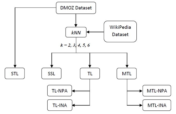
Figure 1: Summary of Evaluated Models. Wikipedia/DMOZ are inter-changeable in the protocol.

Model		$\mu$A$F_{1}$		MAP		MAR		MA$F_{1}$		AMCC
STL		0.5758	(0.0121)	0.7914	(0.0267)	0.6167	(0.0115)	0.6486	(0.0060)	0.6732	(0.0074)
SSL	($k=2$)	0.6178	(0.0160)	0.8064	(0.0413)	0.6649	(0.0125)	0.6789	(0.0231)	0.7048	(0.0263)
	($k=3$)	0.6316	(0.0216)	0.8059	(0.0218)	0.6782	(0.0230)	0.6808	(0.0195)	0.7092	(0.0185)
	($k=4$)	0.6581	(0.0392)	0.8090	(0.0292)	0.6888	(0.0329)	0.6974	(0.0284)	0.7208	(0.0492)
	($k=5$)	0.6719	(0.0540)	0.8091	(0.0406)	0.7093	(0.0314)	0.7045	(0.0152)	0.7359	(0.0064)
	($k=6$)	0.6624	(0.0356)	0.8011	(0.0216)	0.7089	(0.0387)	0.6919	(0.0284)	0.7175	(0.0182)
TL-NPA	($k=2$)	0.5739	(0.0044)	0.7987	(0.0278)	0.6247	(0.0091)	0.6481	(0.0062)	0.6732	(0.0074)
	($k=3$)	0.5728	(0.0103)	0.7893	(0.0128)	0.6250	(0.0126)	0.6480	(0.0081)	0.6737	(0.0171)
	($k=4$)	0.5732	(0.0124)	0.7981	(0.0221)	0.6232	(0.0753)	0.6483	(0.0375)	0.6738	(0.0128)
	($k=5$)	0.5755	(0.0030)	0.8027	(0.0314)	0.6262	(0.0077)	0.6504	(0.0083)	0.6757	(0.0097)
	($k=6$)	0.5738	(0.0462)	0.7413	(0.0593)	0.6096	(0.0522)	0.6248	(0.0563)	0.6631	(0.0387)
TL-INA	($k=2$)	0.5736	(0.0038)	0.7967	(0.0262)	0.6246	(0.0184)	0.6478	(0.0040)	0.6728	(0.0054)
	($k=3$)	0.5810	(0.0731)	0.7918	(0.0137)	0.6182	(0.0126)	0.6488	(0.0031)	0.6794	(0.0138)
	($k=4$)	0.5771	(0.0192)	0.7939	(0.0191)	0.6173	(0.0188)	0.6394	(0.0113)	0.6748	(0.0312)
	($k=5$)	0.5712	(0.0034)	0.8024	(0.0226)	0.6212	(0.0091)	0.6467	(0.0034)	0.6724	(0.0047)
	($k=6$)	0.5700	(0.0144)	0.7853	(0.0268)	0.6132	(0.0164)	0.6298	(0.0372)	0.6489	(0.0189)
MTL-NPA	($k=2$)	0.7442	(0.0201)	0.7819	(0.0356)	0.7840	(0.0169)	0.7373	(0.0349)	0.7527	(0.0335)
	($k=3$)	0.7438	(0.0192)	0.7901	(0.0461)	0.7782	(0.0329)	0.7350	(0.0247)	0.7515	(0.0282)
	($k=4$)	0.7403	(0.0431)	0.7884	(0.0453)	0.7891	(0.0212)	0.7346	(0.0221)	0.7501	(0.0101)
	($k=5$)	0.7394	(0.0219)	0.7720	(0.0421)	0.7814	(0.0140)	0.7293	(0.0318)	0.7488	(0.0298)
	($k=6$)	0.7120	(0.0128)	0.7104	(0.0144)	0.7581	(0.0213)	0.6866	(0.0422)	0.7061	(0.0431)
MTL-INA	($k=2$)	0.7208	(0.0180)	0.7583	(0.0503)	0.7664	(0.0211)	0.7052	(0.0520)	0.7326	(0.0367)
	($k=3$)	0.7294	(0.0213)	0.7592	(0.0101)	0.7616	(0.0473)	0.7070	(0.0211)	0.7313	(0.0312)
	($k=4$)	0.7000	(0.0431)	0.7281	(0.0213)	0.7502	(0.0131)	0.6899	(0.0432)	0.7024	(0.0293)
	($k=5$)	0.7079	(0.0136)	0.7352	(0.0306)	0.7508	(0.0085)	0.6949	(0.0255)	0.7147	(0.0243)
	($k=6$)	0.6992	(0.0721)	0.7271	(0.0721)	0.7321	(0.0632)	0.6797	(0.0413)	0.7024	(0.0339)

• Table shows mean across five runs and (standard deviation) in bracket, standard error for best model: MTL-NPA ($k$ = 2) = 0.0054

Table I: Classification Performance for LD Sample shown for DMOZ dataset.

Model		$\mu$A$F_{1}$		MAP		MAR		MA$F_{1}$		AMCC
STL		0.5236	(0.0989)	0.6415	(0.0741)	0.5213	(0.0998)	0.5318	(0.0625)	0.5837	(0.0782)
SSL	($k=2$)	0.5182	(0.0321)	0.6392	(0.0932)	0.5348	(0.0631)	0.5264	(0.0674)	0.5748	(0.0183)
	($k=3$)	0.5234	(0.0723)	0.6334	(0.0673)	0.5354	(0.0300)	0.5670	(0.0641)	0.5739	(0.0629)
	($k=4$)	0.5329	(0.0631)	0.6312	(0.0681)	0.5360	(0.0810)	0.5698	(0.0524)	0.5802	(0.0285)
	($k=5$)	0.5102	(0.0642)	0.6124	(0.0773)	0.5279	(0.0273)	0.5490	(0.0831)	0.5772	(0.0641)
	($k=6$)	0.5043	(0.0731)	0.6042	(0.0204)	0.5186	(0.0942)	0.5468	(0.0632)	0.5547	(0.0228)
TL-NPA	($k=2$)	0.5418	(0.0182)	0.6682	(0.0136)	0.5633	(0.0362)	0.5823	(0.0317)	0.6930	(0.0831)
	($k=3$)	0.5512	(0.0521)	0.6620	(0.0317)	0.5784	(0.0674)	0.5982	(0.0742)	0.6894	(0.0674)
	($k=4$)	0.5332	(0.0153)	0.6581	(0.0239)	0.5616	(0.0083)	0.5813	(0.0873)	0.6740	(0.0543)
	($k=5$)	0.5295	(0.0743)	0.6327	(0.0854)	0.5610	(0.0674)	0.5704	(0.0029)	0.6649	(0.0895)
	($k=6$)	0.5238	(0.0235)	0.6136	(0.0487)	0.5427	(0.0500)	0.5684	(0.0748)	0.6386	(0.0856)
TL-INA	($k=2$)	0.5368	(0.0573)	0.6734	(0.0198)	0.5464	(0.0563)	0.5982	(0.0130)	0.6946	(0.0846)
	($k=3$)	0.5408	(0.0464)	0.6648	(0.0895)	0.5696	(0.0187)	0.5928	(0.0481)	0.6994	(0.0101)
	($k=4$)	0.5319	(0.0042)	0.6598	(0.0452)	0.5573	(0.0526)	0.5810	(0.0736)	0.6848	(0.0654)
	($k=5$)	0.5278	(0.0674)	0.6394	(0.0895)	0.5210	(0.0183)	0.5624	(0.0901)	0.6740	(0.0538)
	($k=6$)	0.5101	(0.0587)	0.6153	(0.0519)	0.5052	(0.0456)	0.5248	(0.0831)	0.6382	(0.0873)
MTL-NPA	($k=2$)	0.6389	(0.0648)	0.6635	(0.0782)	0.6615	(0.0637)	0.6626	(0.0682)	0.6582	(0.0738)
	($k=3$)	0.6390	(0.0723)	0.6832	(0.0672)	0.6650	(0.0421)	0.6724	(0.0432)	0.6628	(0.0764)
	($k=4$)	0.6283	(0.0748)	0.6624	(0.0613)	0.6593	(0.0382)	0.6602	(0.0936)	0.6585	(0.0631)
	($k=5$)	0.6128	(0.0784)	0.6626	(0.0632)	0.6429	(0.0823)	0.6593	(0.0529)	0.6497	(0.0874)
	($k=6$)	0.6003	(0.0524)	0.6498	(0.0874)	0.6193	(0.0623)	0.6282	(0.0817)	0.6046	(0.0734)
MTL-INA	($k=2$)	0.6120	(0.0629)	0.6448	(0.0325)	0.6428	(0.0618)	0.6432	(0.0663)	0.6420	(0.0728)
	($k=3$)	0.6194	(0.0437)	0.6328	(0.0224)	0.6480	(0.0642)	0.6406	(0.0910)	0.6394	(0.0429)
	($k=4$)	0.6036	(0.0421)	0.6262	(0.0639)	0.6338	(0.0632)	0.6324	(0.0138)	0.6310	(0.0309)
	($k=5$)	0.6040	(0.0101)	0.6160	(0.0819)	0.6282	(0.0192)	0.6202	(0.0328)	0.6290	(0.0456)
	($k=6$)	0.5842	(0.0457)	0.5820	(0.0282)	0.5926	(0.0478)	0.5846	(0.0885)	0.6082	(0.0402)

• Table shows mean across five runs and (standard deviation) in bracket, standard error for best model: MTL-NPA ($k$ = 3) = 0.0087

Table II: Classification Performance for LD sample shown for Wikipedia dataset.

V-A Accuracy Comparison

V-A1 Low distribution sample

Tables I and II show the average performance across five runs for DMOZ and Wikipedia Low Distribution (LD) classes. The following observations can be made from the results.

• STL v/s SSL v/s TL v/s MTL: For both the datasets we see that the MTL methods outperforms all the other methods across all the metrics, exception being in case of LD DMOZ dataset MAP metric. Reason for such exception is high relatedness between the main task and its corresponding neighboring task(s). We also note that among the MTL approaches the Neighborhood Pooling Approach (MTL-NPA) outperformed the Individual Neighborhood Approach (MTL-INA) (statistically significant). Semi-Supervised Learning (SSL) method marginally outperformed both Single Task Learning (STL) as well as Transfer Learning (TL) methods. TL did not seem to have any benefit over STL.

• $k$ = 2 v/s $k$ = 3 v/s $k$ = 4 v/s $k$ = 5 v/s $k$ = 6: In general, lower value of $k$ gave better models compared to higher values of $k$. We conjecture that as the value of $k$ increases, similarity between the main task and the surrogate tasks decreases, which in turn affects the performance negatively.

Model		$\mu$A$F_{1}$		MAP		MAR		MA$F_{1}$		AMCC
STL		0.7592	(0.0120)	0.7947	(0.0068)	0.7618	(0.0056)	0.7567	(0.0085)	0.7626	(0.0075)
SSL	($k=2$)	0.7535	(0.0040)	0.7938	(0.0065)	0.7601	(0.0011)	0.7547	(0.0052)	0.7609	(0.0048)
	($k=3$)	0.7542	(0.0127)	0.7998	(0.0032)	0.7624	(0.0102)	0.7657	(0.0020)	0.7646	(0.0091)
	($k=4$)	0.7512	(0.0031)	0.7972	(0.0084)	0.7618	(0.0090)	0.7592	(0.0029)	0.7628	(0.0075)
	($k=5$)	0.7545	(0.0027)	0.7948	(0.0060)	0.7610	(0.0018)	0.7559	(0.0039)	0.7619	(0.0034)
	($k=6$)	0.7491	(0.0042)	0.7778	(0.0143)	0.7482	(0.0042)	0.7437	(0.0092)	0.7542	(0.0086)
TL-NPA	($k=2$)	0.7536	(0.0042)	0.7936	(0.0054)	0.7588	(0.0015)	0.7546	(0.0048)	0.7610	(0.0043)
	($k=3$)	0.7538	(0.0053)	0.7941	(0.0027)	0.7590	(0.0061)	0.7551	(0.0024)	0.7595	(0.0063)
	($k=4$)	0.7532	(0.0028)	0.7940	(0.0037)	0.7585	(0.0072)	0.7544	(0.0053)	0.7623	(0.0022)
	($k=5$)	0.7533	(0.0038)	0.7937	(0.0063)	0.7584	(0.0024)	0.7542	(0.0052)	0.7605	(0.0046)
	($k=6$)	0.7406	(0.0064)	0.7888	(0.0022)	0.7414	(0.0072)	0.7389	(0.0041)	0.7594	(0.0027)
TL-INA	($k=2$)	0.7529	(0.0040)	0.7958	(0.0054)	0.7591	(0.0011)	0.7540	(0.0048)	0.7603	(0.0043)
	($k=3$)	0.7631	(0.0074)	0.7964	(0.0010)	0.7612	(0.0027)	0.7548	(0.0029)	0.7696	(0.0072)
	($k=4$)	0.7530	(0.0091)	0.7968	(0.0020)	0.7606	(0.0013)	0.7542	(0.0017)	0.7596	(0.0062)
	($k=5$)	0.7527	(0.0038)	0.7957	(0.0046)	0.7590	(0.0010)	0.7538	(0.0036)	0.7602	(0.0042)
	($k=6$)	0.7432	(0.0015)	0.7849	(0.0034)	0.7442	(0.0051)	0.7414	(0.0053)	0.7591	(0.0068)
MTL-NPA	($k=2$)	0.7572	(0.0080)	0.7961	(0.0063)	0.7637	(0.0058)	0.7587	(0.0087)	0.7644	(0.0076)
	($k=3$)	0.7598	(0.0072)	0.7978	(0.0089)	0.7644	(0.0062)	0.7649	(0.0074)	0.7701	(0.0086)
	($k=4$)	0.7571	(0.0035)	0.7964	(0.0076)	0.7632	(0.0093)	0.7584	(0.0102)	0.7640	(0.0054)
	($k=5$)	0.7569	(0.0043)	0.7969	(0.0058)	0.7627	(0.0012)	0.7581	(0.0053)	0.7639	(0.0048)
	($k=6$)	0.7482	(0.0087)	0.7712	(0.0081)	0.7512	(0.0014)	0.7392	(0.0076)	0.7436	(0.0030)
MTL-INA	($k=2$)	0.7579	(0.0103)	0.7978	(0.0076)	0.7644	(0.0079)	0.7599	(0.0111)	0.7657	(0.0099)
	($k=3$)	0.7680	(0.0097)	0.8020	(0.0047)	0.7790	(0.0089)	0.7728	(0.0092)	0.7728	(0.0121)
	($k=4$)	0.7662	(0.0087)	0.8012	(0.0026)	0.7742	(0.0085)	0.7696	(0.0129)	0.7719	(0.0105)
	($k=5$)	0.7657	(0.0067)	0.8017	(0.0073)	0.7717	(0.0037)	0.7678	(0.0081)	0.7726	(0.0072)
	($k=6$)	0.7526	(0.0089)	0.7818	(0.0129)	0.7664	(0.0051)	0.7529	(0.0066)	0.7648	(0.0059)

• Table shows mean across five runs and (standard deviation) in bracket, standard error for best model: MTL-INA ($k$ = 3) = 0.0038

Table III: Classification Performance for HD sample shown for DMOZ dataset.

Model		$\mu$A$F_{1}$		MAP		MAR		MA$F_{1}$		AMCC
STL		0.6648	(0.0628)	0.6841	(0.0630)	0.6429	(0.0089)	0.6748	(0.0172)	0.6881	(0.0120)
SSL	($k=2$)	0.6584	(0.0067)	0.6848	(0.0178)	0.6492	(0.0238)	0.6780	(0.0324)	0.6782	(0.0182)
	($k=3$)	0.6528	(0.0262)	0.6804	(0.0572)	0.6498	(0.0546)	0.6680	(0.0821)	0.6778	(0.0239)
	($k=4$)	0.6530	(0.0287)	0.6768	(0.0231)	0.6400	(0.0262)	0.6612	(0.0387)	0.6704	(0.0263)
	($k=5$)	0.6428	(0.0624)	0.6706	(0.0189)	0.6364	(0.0423)	0.6596	(0.0346)	0.6686	(0.0456)
	($k=6$)	0.6320	(0.0822)	0.6700	(0.0037)	0.6342	(0.0892)	0.6502	(0.0521)	0.6648	(0.0190)
TL-NPA	($k=2$)	0.6628	(0.0636)	0.6820	(0.0976)	0.6528	(0.0174)	0.6792	(0.0733)	0.6840	(0.0785)
	($k=3$)	0.6614	(0.0463)	0.6838	(0.0842)	0.6510	(0.0597)	0.6797	(0.0471)	0.6888	(0.0823)
	($k=4$)	0.6528	(0.0367)	0.6735	(0.0963)	0.6482	(0.0871)	0.6626	(0.0913)	0.6710	(0.0731)
	($k=5$)	0.6500	(0.0689)	0.6629	(0.0729)	0.6285	(0.0463)	0.6389	(0.0582)	0.6618	(0.0838)
	($k=6$)	0.6450	(0.0893)	0.6482	(0.0572)	0.6021	(0.0578)	0.6124	(0.0527)	0.6484	(0.0657)
TL-INA	($k=2$)	0.6531	(0.0462)	0.6623	(0.0572)	0.6482	(0.0863)	0.6504	(0.0427)	0.6731	(0.0865)
	($k=3$)	0.6512	(0.0845)	0.6547	(0.0864)	0.6273	(0.0974)	0.6397	(0.0645)	0.6682	(0.0472)
	($k=4$)	0.6510	(0.0467)	0.6524	(0.0246)	0.6244	(0.0755)	0.6326	(0.0624)	0.6539	(0.0573)
	($k=5$)	0.6427	(0.0533)	0.6510	(0.0217)	0.6218	(0.0381)	0.6304	(0.0256)	0.6512	(0.0972)
	($k=6$)	0.6308	(0.0572)	0.6404	(0.0384)	0.6036	(0.0330)	0.6198	(0.0472)	0.6380	(0.0753)
MTL-NPA	($k=2$)	0.6620	(0.0672)	0.6824	(0.0317)	0.6428	(0.0871)	0.6704	(0.0174)	0.6868	(0.0623)
	($k=3$)	0.6702	(0.0053)	0.6826	(0.0183)	0.6440	(0.0542)	0.6748	(0.0831)	0.6880	(0.0542)
	($k=4$)	0.6634	(0.0184)	0.6782	(0.0172)	0.6210	(0.0281)	0.6529	(0.0600)	0.6693	(0.0622)
	($k=5$)	0.6608	(0.0731)	0.6616	(0.0722)	0.6201	(0.0193)	0.6500	(0.0783)	0.6524	(0.0734)
	($k=6$)	0.6529	(0.0620)	0.6583	(0.0318)	0.6183	(0.0731)	0.6472	(0.0561)	0.6510	(0.0582)
MTL-INA	($k=2$)	0.6720	(0.0134)	0.6898	(0.0531)	0.6548	(0.0146)	0.6784	(0.0142)	0.6898	(0.0712)
	($k=3$)	0.6717	(0.0108)	0.6864	(0.0142)	0.6550	(0.0398)	0.6772	(0.0152)	0.6720	(0.0256)
	($k=4$)	0.6683	(0.0040)	0.6747	(0.0051)	0.6484	(0.0193)	0.6696	(0.0641)	0.6704	(0.0138)
	($k=5$)	0.6601	(0.0839)	0.6630	(0.0931)	0.6418	(0.0322)	0.6642	(0.0412)	0.6652	(0.0313)
	($k=6$)	0.6539	(0.0713)	0.6565	(0.0172)	0.6402	(0.0742)	0.6598	(0.0193)	0.6584	(0.0105)

• Table shows mean across five runs and (standard deviation) in bracket, standard error for best model: MTL-INA ($k$ = 2) = 0.0068

Table IV: Classification Performance for HD sample shown for Wikipedia dataset.

V-A2 High distribution sample

Table III and IV show the average performance across five runs for DMOZ and Wikipedia High Distribution (HD) classes. We make the following observations based on the results.

• STL v/s SSL v/s TL v/s MTL: In this case we see that the MTL methods perform only slightly better than other models, the differences are not statistically significant. This supports our intuition that with sufficient number of examples for learning the SSL, TL and MTL methods do not provide any distinct advantage and the simple STL model is competitive.

• $k$ = 2 v/s $k$ = 3 v/s $k$ = 4 v/s $k$ = 5 v/s $k$ = 6: As with the case of Low Distribution classes, we noticed a slight degradation of performance as the number of neighbors is increased.

V-B Run time Comparison

Table V shows the average training time (in sec.) per class required to learn the models for the different LD and HD categories. The STL approach has the lowest training times because there is no overhead of incorporating additional constraints is involved. SSL models takes more time than the corresponding STL models because of the increased number of training examples. For TL models as well, run time increases because it requires learning the models for the neighbors. Finally, MTL method takes the longest time, since it requires the joint learning of the model parameters that are updated for each class and related neighbors.

		DMOZ		Wiki
Model		LD	HD	LD	HD
STL		2.72	44.7	2.84	46.7
SSL	($k=2$)	4.58	62.4	8.64	68.3
	($k=4$)	5.57	62.7	9.73	70.5
	($k=6$)	6.48	64.3	10.6	73.0
TL-NPA	($k=2$)	4.65	48.6	10.2	70.7
	($k=4$)	6.3	52.6	13.6	74.6
	($k=6$)	7.5	56.1	15.5	78.8
TL-INA	($k=2$)	4.54	48.4	12.6	72.6
	($k=4$)	6.40	50.3	14.6	76.8
	($k=6$)	7.98	54.7	15.6	80.7
MTL-NPA	($k=2$)	5.51	49.5	12.6	69.6
	($k=4$)	7.53	54.2	14.5	70.3
	($k=6$)	8.75	58.1	15.8	72.4
MTL-INA	($k=2$)	9.84	56.8	17.8	78.7
	($k=4$)	15.6	78.7	19.3	84.7
	($k=6$)	18.8	82.8	22.3	92.4

Table V: Run time (in sec.) comparison (Reported per class across five runs)

VI Conclusion and Future Work

In this paper we developed Multi-task Learning models for text document classification. Performance of the MTL methods was compared with Single Task Learning, Semi-supervised Learning and Transfer Learning approaches. We compared the methods in terms of accuracy and run-times. MTL methods outperformed the other methods, especially for the Low Distribution classes, where the number of positive training examples was small. For the High Distribution classes with sufficient number of positive training examples, the performance improvement was not noticeable.

Datasets organize information as hierarchies. We plan to extract the parent-child relationships existing within the DMOZ and Wikipedia hierarchies to improve the classification performance. We also plan to use the accelerated/proximal gradient descent approach to improve the learning rates. Finally, we also seek to improve run-time performance by implementing our approaches using data parallelism, seen in GPUs.

VII Acknowledgement

This project was funded by NSF career award 1252318.

References

- [1] J. Zhou, L. Yuan, J. Liu, and J. Ye. A multi-task learning formulation for predicting disease progression. Proceedings of the 17th ACM SIGKDD international conference on Knowledge discovery and data mining, ACM, 2011.
- [2] Anveshi Charuvaka and Huzefa Rangwala. Multi-task learning for classifying proteins with dual hierarchies. pages 834–839, 12/2012 2012.
- [3] C. Widmer, J. Leiva, Y. Altun, and G. Rätsch. Leveraging sequence classification by taxonomy-based multitask learning. 14th Annual International Conference, RECOMB, Lisbon, Portugal, pages 522–534, April 25-28, 2010.
- [4] X. Wang, C. Zhang, and Z. Zhang. Boosted multi-task learning for face verification with applications to web image and video search. IEEE conference on Computer Vision and Pattern Recognition, pages 142–149, 2009.
- [5] R. Caruana. Multitask learning. Machine Learning, 28(1):41–75, 1997.
- [6] J. Baxter. A model of inductive bias learning. JAIR, 12:149–198, 2000.
- [7] S. Thrun. Is learning the n-th thing any easier than learning the first? NIPS, pages 640–646, 1996.
- [8] S. Ben-David and R. Schuller. Exploiting task relatedness for multiple task learning. Learning Theory and Kernel Machines, pages 567–580, 2003.
- [9] J. Zhou, J. Chen, and J. Ye. MALSAR: Multi-tAsk Learning via StructurAl Regularization. Arizona State University, 2011.
- [10] T. Evgeniou and M. Pontil. Regularized multitask learning. KDD, pages 109–117, 2004.
- [11] T. Jebara. Multitask sparsity via maximum entropy discrimination. JMLR, pages 75–110, 2011.
- [12] A. Argyriou, T. Evgeniou, and M. Pontil. Convex multi-task feature learning. Machine Learning, 73(3):243–272, 2008.
- [13] J. Liu, S. Ji, and J. Ye. Multi-task feature learning via efficient l 2, 1-norm minimization. UIA, pages 339–348, 2009.
- [14] G. Obozinski, B. Taskar, and M. Jordan. Multi-task feature selection. ICML, 2006.
- [15] R. Tibshirani. Regression shrinkage and selection via the lasso. Journal of the Royal Statistical Society. Series B (Methodological), pages 267–288, 1996.
- [16] A. Argyriou, T. Evgeniou, and M. Pontil. Multi-task feature learning. NIPS, page 19:41, 2007.
- [17] T. Jebara. Multi-task feature and kernel selection for svms. ICML, page 55, 2004.
- [18] T. Kato, H. Kashima, M. Sugiyama, and K. Asai. Multi-task learning via conic programming. NIPS, pages 737–744, 2008.
- [19] T. Evgeniou, C.A. Micchelli, and M. Pontil. Learning multiple tasks with kernel methods. JMLR, 6(1):615–637, 2005.
- [20] S. Thrun and J. O. Sullivan. Clustering learning tasks and the selective cross-task transfer of knowledge. Learning to learn, pages 181–209, 1998.
- [21] L. Jacob, F. Bach, and J.P. Vert. Clustered multi-task learning: A convex formulation. NIPS, 2008.
- [22] J. Zhou, J. Chen, and J. Ye. Clustered multi-task learning via alternating structure optimization. NIPS, 2011.
- [23] E. Bonilla, K.M. Chai, and C. Williams. Multi-task gaussian process prediction. NIPS, 20(October), 2008.
- [24] Y. Zhang and D.Y. Yeung. A convex formulation for learning task relationships in multi-task learning. In Proceedings of the Twenty-fourth Conference on Uncertainty in AI (UAI), 2010.
- [25] S.J. Pan and Q. Yang. A survey on transfer learning. IEEE Transactions on Knowledge and Data Engineering, 22(10):1345–1359, 2010.
- [26] N. Bhatia and Vandana. Survey of nearest neighbor techniques. International Journal of Computer Science and Information Security, 8(2):302–305, 2010.
- [27] X. Zhu. Semi-supervised learning literature survey. world, 10:10, 2005.
- [28] Azad Naik. Using multi-task learning for large-scale document classification. Master’s thesis, George Mason University, Fairfax, Virginia (USA), 2013.
- [29] Y. Yang. An evaluation of statistical approaches to text categorization. Information Retrieval, 1(1):69–90, 1999.
- [30] D. Lewis, R. Schapire, J. Callan, and R. Papka. Training algorithms for linear text classifiers. pages 298–306, New York, 1996.
- [31] A. Özgür, L. Özgür, and T. Güngör. Text categorization with class-based and corpus-based keyword selection. Proceedings of the 20th international conference on Computer and Information Sciences, pages 606–615, 2005.
- [32] P. Baldi, S. Brunak, Y. Chauvin, C.A.F. Andersen, and H. Nielsen. Assessing the accuracy of prediction algorithms for classification: an overview. Bioinformatics, 16(5):412–424, 2000.