ToPs: Ensemble Learning with Trees of Predictors

Abstract

We present a new approach to ensemble learning. Our approach differs from previous approaches in that it constructs and applies different predictive models to different subsets of the feature space. It does this by constructing a tree of subsets of the feature space and associating a predictor (predictive model) to each node of the tree; we call the resulting object a tree of predictors. The (locally) optimal tree of predictors is derived recursively; each step involves jointly optimizing the split of the terminal nodes of the previous tree and the choice of learner (from among a given set of base learners) and training set – hence predictor – for each set in the split. The features of a new instance determine a unique path through the optimal tree of predictors; the final prediction aggregates the predictions of the predictors along this path. Thus, our approach uses base learners to create complex learners that are matched to the characteristics of the data set while avoiding overfitting. We establish loss bounds for the final predictor in terms of the Rademacher complexity of the base learners. We report the results of a number of experiments on a variety of datasets, showing that our approach provides statistically significant improvements over a wide variety of state-of-the-art machine learning algorithms, including various ensemble learning methods.

I Introduction

Ensemble methods [1, 2, 3, 4] are general techniques in machine learning that combine several learners; these techniques include bagging [5, 6, 7], boosting [8, 9] and stacking [10]. Ensemble methods frequently improve predictive performance. We describe a novel approach to ensemble learning that chooses the learners to be used, the way in which these learners should be trained to create predictors (predictive models), and the way in which the predictions of these predictors should be combined according to the features of a new instance for which a prediction is desired. By jointly deciding which learners and training sets to be used, we provide a novel method to grow complex predictors; by deciding how to aggregate these predictors we control overfitting. As a result, we obtain substantially improved predictive performance.

Our proposed model, ToPs (Trees of Predictors), differs from existing methods in that it constructs and applies different predictive models to different subsets of the feature space. Our approach has something in common with tree-based approaches (e.g. Random forest, Tree-bagging, CART, etc.) in that we successively split the feature space. However, while tree-based approaches create successive splits of the feature space in order to maximize homogeneity of each split with respect to labels, ToPs creates successive splits of the feature space in order to maximize predictive accuracy of each split with respect to a constructed predictive model. To this end, ToPs creates a tree of subsets of the feature space and associates a predictive model to each such subset – i.e., to each node of the tree. To decide whether to split a given node, ToPs uses a feature to create a tentative split, then chooses a learner and a training set to create a predictive model for each set in the split, and searches for the feature, the learner and the training set that maximizes the predictive accuracy (minimizes the prediction error). ToPs continues this process recursively until no further improvement is possible.

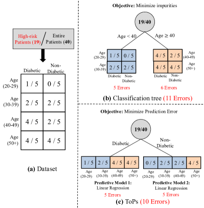
Figure 1: Toy example. (a) Dataset, (b) Classification tree, (c) ToPs

A simple toy example, illustrated in Fig. 1, may help to illustrate how ToPs works and why it improves on other tree-based methods. We consider a classification problem: making binary predictions of hypertension in a patient population. We assume two features: Diabetic or Non-diabetic and Age Range 20-29, 30-39, 40-49, 50+, so that there are 8 categories of patients. We assume the data is as shown in Fig. 1 (a): there are 5 patients in each category; 1 patient who is Diabetic and in the Age Range 20-29 has hypertension, etc. We first consider a simple classification tree. Such a tree first selects a single feature and threshold to split the population into two groups so as to maximize the purity of labels. In this case the best split uses Age Range as the splitting feature and partitions patients into those in the Age Ranges 20-29 or 30-39 and those in the Age Ranges 40-49 or 50+. No further splitting improves the purity of labels so we are left with the tree shown in Fig. 1 (b). The resulting predictive model predicts that those in the Age Ranges 20-29 or 30-39 will not have hypertension and those in the Age Ranges 40-49 or 50+ will have hypertension; this model makes 11 prediction errors. We now consider an instantiation of ToPs which uses as base learner a linear regression (to produce a probability of hypertension) followed by thresholding at 0.5. (Recall that we are treating this as a classification problem.) The best split for this instantiation of ToPs uses Diabetic/Non-diabetic as the splitting feature (leading to the split shown in Fig. 1 (c)) but creates different predictive models in the two halves of the split: in the Non-diabetic half of the split, the model predicts that patients in the Age Ranges 20-29, 30-39 and 40-49 will not have hypertension and that patients in the Age Range 50+ will have hypertension; in the Diabetic half of the split the model predicts that patients in the Age Ranges 20-29 and 30-39 will not have hypertension and that patients in the Age Ranges 40-49 and 50+ will have hypertension. (After this split, no further splits using this single base learner improve the prediction accuracy.) This model makes only 10 errors (less than the number of errors made by the classification tree). Note that the tree produced by ToPs is completely different from the classification tree, that the predictive models and predictions produced by ToPs are different from those produced by the classification tree, and that the predictions produced by ToPs within a single terminal node are not uniform. In this case, ToPs performs better than the classification tree because it "understands" that the effect of age on the risk of hypertension is different for patients who are Diabetic and for patients who are Non-diabetic.

Although this toy example may seem artificial, it exemplifies what happens when we apply ToPs to a real dataset. For example, one of our experiments is survival prediction of patients who are wait-listed for a heart transplant. (For more discussion, see Section V and VI.) In that setting features $X$ are patient characteristics and labels $Y$ are survival times. The data set ${D}$ consists of records of actual patients; a single data point $(x^{t},y^{t})$ records that a patient with features $x^{t}$ survived for time $y^{t}$. The construction of our algorithm demonstrates that the best predictor of survival for males is different from the best predictor of survival for females. As a result, predictions of survival for a male and a female with otherwise similar features may be quite different - because the features that influence survival have different importance and interact differently for males and females. Using a gender-specific predictor leads to significant improvement in prediction accuracy.

In what follows, Section II highlights the differences between our method and related machine learning methods. Section III provides a full description of our method. Section IV derives loss bounds. Section V compares the performance of our method with that of many other methods on a variety of datasets, demonstrating that our method provides substantial and statistically significant improvement. Section VI details the operation of our algorithm for one of the datasets to further illustrate how why our method works. Section VII concludes. Proofs are in the Appendix (at the end of the manuscript); parameters of the experiments and additional figures and discussion can be found in the Supplementary Materials.

TABLE I: Comparison with existing methods

Methods	Sub-categories	Approach of existing methods	Approach of ToPs
Ensemble Methods	Bagging, Boosting, Stacking	Construct multiple predictive models (with single learning algorithm) using randomly selected training sets.	Construct multiple predictive models using multiple learning algorithms and optimal training sets.
		Only the predictive models are optimized to minimize the loss.	Training sets and the assigned predictive model for each training set are jointly optimized to minimize the loss
Tree-based Methods	Decision Tree, Regression tree	Grow a tree by choosing the split that minimizes the impurities of labels in each node.	Grow a tree by choosing the split that minimizes the prediction error of the best predictive models.
		Within a single terminal node all the predictions are uniform (identical) .	Within a single terminal node, the final predictive model is uniform but the predictions can be different.
Non-parametric Regression	Gaussian Process, Kernel Regression	Construct a non-parametric predictive model with pre-determined kernels using the entire training set.	Construct non-parametric predictive models by jointly optimizing the training sets and the best predictive models.
		Similarities between data points are fixed functions of the features.	Similarities between data points are determined by the prediction errors.
Model trees	[12], [13], [14], [15], [16]	Construct the tree by jointly optimizing a (single) learning algorithm and the splits	Construct the tree by jointly optimizing multiple learning algorithms and the splits
		Only convex loss functions are allowed.	Arbitrary loss functions such as AUC are allowed.
		The final prediction for a new instance depends only on the terminal node to which the feature of the instance belongs.	The final prediction is a weighted average of the predictions along all the nodes to which the feature of the instance belong (the path to the terminal node).

II Methodological Comparisons

ToPs is most naturally compared with four previous bodies of work: model trees, other tree-based methods, ensemble methods, and non-parametric regression. Table I summarizes the comparisons with existing methods. The optimization equations of existing works are also compared in the Appendix Table V.

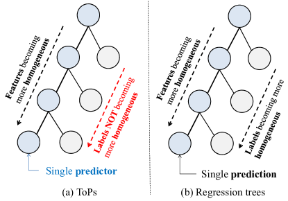
Figure 2: The main differences between ToPs and regression trees. (a) ToPs, (b) regression trees

II-A Model trees

There are similarities between ToPs and model trees but also very substantial differences. The initial papers on model trees [11, 12] construct a tree using a splitting criterion that depends on labels but not on predictions, then prunes the tree, using linear regression at a node to replace subtrees from that node. [13] constructs the tree in the same way but allows for more general learners when replacing subtrees from a node. [14, 15] split the tree by jointly optimizing a linear predictive model and the splits that minimize the loss or maximize the statistical differences between two splits.

ToPs operates differently from all of these: it constructs the tree using a splitting criterion that depends both on labels and on predictions of its base learners, it does not prune its tree nor does it replace any subtree with a predictive model.

In ToPs, the potential split of a node is evaluated by training each base learner on the current node and on all parent nodes (not just the current node, as in [14, 15]) and choosing the split and the predictor that yield the best overall performance. (Keep in mind that ToPs is a general framework that allows for an arbitrary set of base learners.) This approach is important for several reasons: (1) It avoids the problem of small training sets and reduces overfitting. (2) It allows splits even when only one side of the split yields an improved performance. (3) It allows for choosing the base learner among multiple learners that best capture the importance of features and the interactions among features. ToPs constructs the final prediction as a weighted average of predictions along the path (with weights determined by linear regression). Weighted averaging is important because it smooths the prediction, from the least biased model to the most biased model. Determining the weights by linear regression is important because it is an optimizing procedure, and so the weights depend on the data and on the accuracy of the predictors constructed. ([15] also smooths by weighted averaging but chooses the weights according to the number of samples and number of features. This makes sense only with a single base learner and hence a single model complexity. With multiple models of different model complexities, it is impossible to find the appropriate aggregation weights using only the number of features and number of samples). Finally, the construction of ToPs allows for arbitrary loss functions, including loss functions such as AUC that are not sample means. This is important because loss functions such as AUC are especially appropriate for certain applications; e.g. survival in the heart transplant dataset.

II-B Other tree-based methods

Decisions trees, regression trees [16], tree bagging, and random forest [5] follow a recursive procedure, growing a tree by using features to create tentative splits and labels to choose among the tentative splits. Eventually, these methods create a final partition (the terminal nodes of the tree) and make a single uniform prediction within each set of this partition. Some of these methods construct multiple trees and hence multiple partitions and aggregate the predictions arising from each partition. Our method also follows a recursive procedure, growing a tree by using features to create tentative splits, but we then use features and labels and predictors to choose the optimal split and associated predictors. Eventually, we produce a (locally) optimal tree of predictors. The final prediction for a given new instance is computed by aggregating the predictions along a path in this tree of predictors. A crucial difference between other tree-based methods and ToPs is the treatment of instances that give rise to the same paths: in other tree-based methods, such instances will be assigned the same prediction; in ToPs, such instances will be assigned the same predictor but may be assigned very different predictions. Other tree-based models have the property that within a single terminal node all the predictions are uniform; ToPs has the property that within a single terminal node the predictor is uniform but the predictions can be different. See again the illustrative example above and Fig. 2. (ToPs also has something - but less - in common with hierarchical logistic regression and hierarchical trees; in view of space constraints we defer the discussion to the Supplementary Materials.)

II-C Ensemble methods

Bagging [17], boosting [9, 18, 19, 20], stacking [10, 21] construct multiple predictive models using different training sets and then aggregate the predictions of these models according to endogenously determined weights. Bagging methods use a single base learner and choose random training sets (ignoring both features and labels). Boosting methods use a single base learner and choose a sequence of training sets to create a sequence of predictive models; the sequence of training sets is created recursively according to random draws from the entire training set but weighted by the errors of the previous predictive model. Stacking uses multiple base learners with a single training set to construct multiple predictive models and then aggregates the predictions of these multiple predictive models. Our method uses a recursive construction to construct a locally optimal tree of predictors, using both multiple base learners and multiple training sets and constructs optimal weights to aggregate the predictions of these predictors.

II-D Non-parametric regressions

Kernel regression [22, 23] and Gaussian process regression [24] have in common that given a feature $x$, they choose a training set and use that set to determine the coefficients of a linear learner/model to predict the label $y$. Kernel regression begins with a parametric family of kernels $\{K_{\theta}\}$. For a specific vector $\theta$ of parameters and a specific bandwidth $b$, the regression considers the set $B$ of data points $(x^{t},y^{t})$ whose feature $x^{t}$ are within the specified bandwidth $b$ of $x$; the predicted value of the corresponding label $y$ is the weighted sum $\sum_{B}K_{\theta}(x,x^{t})\,y^{t}$. The optimal parameter $\theta^{*}$ and bandwidth $b^{*}$ can be set by training, typically using least squared error as the optimization criterion. Gaussian process regression begins by assuming a Gaussian form for the kernel but with unknown mean and variance. It first uses a maximum likelihood estimator based on the entire data set to determine the mean and variance (and perhaps a bandwidth), and then uses that the Gaussian kernel to carry out a kernel regression. In both kernel regression and Gaussian process regression, the prediction for a new instance is formed by aggregating the labels associated to nearby features. In our method, the prediction for a new instance is formed by carefully aggregating the predictions of a carefully constructed family of predictors.

III ToPs

We work in a supervised setting so data is presented as a pair $(x,y)$ consisting of a feature and a label. We are presented with a (finite) dataset ${D}=\{(x^{t},y^{t})\}$, assumed to be drawn iid from the true distribution ${\mathcal{D}}$, and seek to learn a model that predicts, for a new instance drawn from ${\mathcal{D}}$ and for which we observe the feature vector $x$, the true label $y$. We assume the space of features is $X=X_{1}\times\cdots X_{d}$; if $x\in X$ then $x_{i}$ is the $i$-th feature. Some features are categorical, others are continuous. For convenience (and without much loss of generality) we assume categorical features are binary and represented as $0,1$ and that continuous features are normalized between $0,1$; hence $X_{i}\subset[0,1]$ for every $i$ and $X\subset[0,1]^{d}$. We also take as given a set $Y\subset{\mathbb{R}}$ of labels. For $Z\subset X$, a predictor (predictive model) on $Z$ is a map $h:Z\to Y$ or $h:Z\to\mathbf{R}$; we interpret $h(z)$ as the predicted label or the expectation of the predicted label, given the feature $z$. (We often suppress $Z$ when $Z=X$ or when $Z$ is understood.) If $h_{1}:Z_{1}\to Y,h_{2}:Z_{2}\to Y$ are predictors and $Z_{1}\cap Z_{2}=\emptyset$ we define $h_{1}\vee h_{2}:Z_{1}\cup Z_{2}\to Y$ by $h_{1}\vee h_{2}(z)=h_{i}(z)$ if $z\in Z_{i}$. All the notations are summarized in the nomenclature table (Table II).

TABLE II: Nomenclature table

Symbol	Explanation
$\mathcal{A}$	A set of algorithms
$A$	An algorithm ($\in\mathcal{A}$)
$C$	A node
$C^{\uparrow}$	Set consisting of node $C$ and all its predecessors
$\bar{C}(x)$	The unique terminal node that contains $x$
$C^{+},C^{-}$	Divided subsets (Similarly for $h,A,S$ and $V$)
$D$	Dataset $=\{(x^{t},y^{t})\}$
$\mathcal{D}$	True distribution
$h_{C}$	Predictive model assigned to $C$
$H(x)$	Overall prediction assigned to $x$ by the overall predictor $H$
$L(h,Z)$	The loss with a predictor $h$ and the set $Z$
$M$	Number of algorithms
$N$	Number of samples
$\Pi(x)$	Path from the initial node to the terminal node with $x$
$S$	Training set
$\tau$	Threshold to divide nodes
$\mathcal{T}$	A tree
$\bar{\mathcal{T}}$	Set of terminal nodes
$V^{1},V^{2}$	Two validation sets
$w^{*}(C,\Pi)$	Weights of $C$ on the path $\Pi$
$X$	Feature space
$(x^{t},y^{t})$	Instance. $x^{t}$: feature, $y^{t}$: label
$x_{i}$	$i$-th feature
$Y$	Label set
$Z$	Subspace of the feature space

We take as given a finite family ${\mathcal{A}}=\{A_{1},\ldots,A_{M}\}$ of algorithms or base learners. We interpret an algorithm as including the parameters of that algorithm (if any); thus Random Forest with 100 trees is a different algorithm than Random Forest with 200 trees. Given an algorithm $A\in{\mathcal{A}}$ and a set $E\subset{D}$ to be used to train $A$, we write $A(E)$ for the resulting predictor. If $\mathcal{E}$ is a family of subsets of ${D}$ then we write ${\mathcal{A}}({\mathcal{E}})=\{A(E):A\in{\mathcal{A}},E\in{\mathcal{E}}\}$ for the set of predictors that can arise from training some algorithm in ${\mathcal{A}}$ on some set in $\mathcal{E}$.

A tree of predictors is a pair $({\mathcal{T}},\{h_{C}\})$ consisting of a (finite) family ${\mathcal{T}}$ of non-empty subsets of $X$ together with an assignment $C\mapsto h_{C}$ of a predictor $h_{C}$ on $C$ to each element $C\in{\mathcal{T}}$ such that:

1. $X\in{\mathcal{T}}$.

2. With respect to the ordering induced by set inclusion, ${\mathcal{T}}$ forms a tree; i.e., ${\mathcal{T}}$ is partially ordered in such a way that each $C\in{\mathcal{T}}$, $C\not=X$ has a unique immediate predecessor. As usual, we refer to the elements of ${\mathcal{T}}$ as nodes. Note that $X$ is the initial node.

3. If $C\in{\mathcal{T}}$ is not a terminal node then the set $C^{\rm succ}$ of immediate successors of $C$ is a partition of $C$.

4. For each node $C\in{\mathcal{T}}$ there is an algorithm $A_{C}\in{\mathcal{A}}$ and a node $C^{*}\in{\mathcal{T}}$ such that $C\subset C^{*}$ (so that either $C=C^{*}$ or $C^{*}$ precedes $C$ in ${\mathcal{T}}$) and $h_{C}=A_{C}(C^{*})$ is the predictor formed by training the algorithm $A_{C}$ on the training set $C^{*}$.

It follows from these requirements that for any two nodes $C_{1},C_{2}\in{\mathcal{T}}$ exactly one of the following must hold: $C_{1}\subset C_{2}$ or $C_{2}\subset C_{1}$ or $C_{1}\cap C_{2}=\emptyset$. It also follows that the set of terminal nodes forms a partition of $X$. For any node $C$ we write $C^{\uparrow}$ for the set consisting of $C$ and all its predecessors. For $\in X$ we write $\overline{C}(x)$ for the unique terminal node that contains $x$ and $\Pi(x)=\Pi(\overline{C}(x))$ for the unique path in ${\mathcal{T}}$ from the initial node $X$ to the terminal node $\overline{C}(x)$. We write $\overline{{\mathcal{T}}}$ for the set of all terminal nodes.

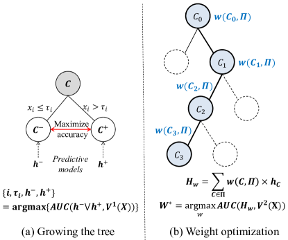
Figure 3: Illustrations of ToPs (a) growing the tree, (b) weight optimization

We fix a partition of the given dataset ${D}=S\cup V^{1}\cup V^{2}$; we view $S$ as the (global) training set and $V^{1},V^{2}$ as (global) validation sets. In practice, the partition of ${D}$ into training and validation sets will be chosen randomly. Given a set $C\subset X$ of feature vectors and a subset $Z\subset{D}$, write $Z(C)=\{(x^{t},y^{t})\in Z:x^{t}\in C\}$.

We express performance in terms of loss. For many problems, an appropriate measure of performance is the Area Under the (receiver operating characteristic) Curve (AUC); for a given set of data $Z\subset D$ and predictor $h:Z(X)\to Y$ the loss is $L(h,Z)=1-AUC$. For other problems, an appropriate measure of loss is the sample mean error $L(h,Z)=\frac{1}{|Z|}\sum_{(x,y)\in Z}|h(x)-y|$. For our general model, we allow for an arbitrary loss function. Given disjoint sets $Z_{1},\ldots,Z_{N}$ and predictors $h_{n}$ on $Z_{n}$, we measure the total (joint) loss as $L(\bigvee h_{n},\bigcup Z_{n})$. Note that the loss function need not be additive, so in general $L(\bigvee h_{n},\bigcup Z_{n})\not=\sum L(h_{n},Z_{n})$

III-A Growing the (Locally) Optimal Tree of Predictors

We begin with the (trivial) tree of predictors $(\{X\},\{h_{X}\})$ where $h_{X}$ is the predictor $h\in{\mathcal{A}}(\{S\})$ that minimizes the loss $L(h,V^{1}(X))$. Note that we train $h$ globally – on the entire training set - and evaluate/validate it globally - on the entire (first) validation set - because the initial node consists of the entire feature space. We now grow the tree of predictors by a recursive splitting process, which is illustrated in Fig. 3 (a). Fix the tree of predictors $({\mathcal{T}},\{h_{C}\})$ constructed to this point. For each terminal node $C\in{\mathcal{T}}$ with its associated predictor $h_{C}$, choose a feature $i$ and a threshold $\tau_{i}\in[0,1]$. (In practice, for binary variables, the threshold is set at 0.5. For continuous variables, the thresholds are set to delineate percentile boundaries at 10% and 90%, with increments of 10%.) Write

$$C^{-}(\tau_{i}) =\{x\in C:x_{i}<\tau_{i}\}$$

$$C^{+}(\tau_{i}) =\{x\in C:x_{i}\geq\tau_{i}\}$$

Evidently $C^{-}(\tau_{i}),C^{+}(\tau_{i})$ are disjoint and $C=C^{-}(\tau_{i})\cup C^{+}(\tau_{i})$, so we are splitting $C$ according to the feature $i$ and the threshold $\tau_{i}$. Note that $C^{-}(\tau_{i})=\emptyset$ if $\tau_{i}=0$; in this case we are not properly splitting $C$. For each of $C^{-}(\tau_{i}),C^{+}(\tau_{i})$ we choose predictors $h^{-}\in{\mathcal{A}}(C^{-}(\tau_{i})^{\uparrow}),h^{+}\in{\mathcal{A}}(C^{+}(\tau_{i})^{\uparrow})$. (That is, we choose predictors that arise from one of the learners $A\in{\mathcal{A}}$, trained on some node that (weakly) precedes the given node.) We then choose the feature $i^{*}$, the threshold $\tau_{i}^{*}$, and the predictors $h_{C^{-}(\tau_{i}^{*})},h_{C^{+}(\tau_{i}^{*})}$ to minimize the total loss on $V^{1}$; i.e. we choose them to solve the minimization problem

$$\arg\min_{i,\tau_{i},h^{-},h^{+}}L\Bigl{(}h^{-}\vee h^{+},V^{1}\bigl{(}C^{-}(\tau_{i})\bigr{)}\cup V^{1}\bigl{(}C^{+}(\tau_{i})\bigr{)}\Bigr{)}$$

subject to the requirement that this total loss should be strictly less than $L(h_{C},V^{1}(C))$. Note that because choosing the threshold $\tau_{i}=0$ does not properly split $C$, the loss $L(h_{C},V^{1}(C))$ can always be achieved by setting $\tau_{i}=0$ and $h^{+}=h_{C}$. If there is no proper splitting that yields a total loss smaller than $L(h_{C},V^{1}(C))$ we do not split this node. This yields a new tree of predictors. We stop the entire process when no terminal node is further split; we refer to the final object as the locally optimal tree of predictors. (We use the adjective "locally" because we have restricted the splitting to be by a single feature and a single threshold and because the optimization process employs a greedy algorithm – it does not look ahead.)

Algorithm 1 Growing the Optimal Tree of Predictors

  Input: Feature space $X$, a set of algorithms ${\mathcal{A}}$, training set $S$, the first validation set $V^{1}$

  First step:

  Initial tree of predictors $=(X,h_{X})$,

  where $h_{X}=\arg\min_{A\in{\mathcal{A}}}L(A(S),V^{1})$

  Recursive step:

  Input: Current tree of predictors ($({\mathcal{T}},\{h_{C}\}$)

  For each terminal node $C\in\mathcal{T}$

     For a feature $i$ and a threshold $\tau_{i}\in[0,1]$.

       Set $C^{-}(\tau_{i})=\{x\in C:x_{i}<\tau_{i}\}$

            $C^{+}(\tau_{i})=\{x\in C:x_{i}\geq\tau_{i}\}$

       Then,

       $\{i^{*},\tau_{i}^{*},h_{C^{-}(\tau_{i}^{*})},h_{C^{+}(\tau_{i}^{*})}\}=$

       ${\rm arg}\min L\Bigl{(}h^{-}\vee h^{+},V^{1}\bigl{(}C^{-}(\tau_{i})\bigr{)}\cup V^{1}\bigl{(}C^{+}(\tau_{i})\bigr{)}\Bigr{)}$

       where $h^{-}\in{\mathcal{A}}(C^{-}(\tau_{i})^{\uparrow}),h^{+}\in{\mathcal{A}}(C^{-}(\tau_{i})^{\uparrow})$

     End For

  End For

  Stopping criterion:

  $L(h_{C},V^{1}(C))\leq$

  $\min L\Bigl{(}h^{-}\vee h^{+},V^{1}\bigl{(}C^{-}(\tau_{i})\bigr{)}\cup V^{1}\bigl{(}C^{+}(\tau_{i})\bigr{)}\Bigr{)}$

  Output: Locally optimal tree of predictors (${\mathcal{T}},\{h_{C}\})$

III-B Weights on the Path

Fix the locally optimal tree of predictors$({\mathcal{T}},\{h_{C}\})$ and a terminal node $\overline{C}$; let $\Pi$ be the path from $X$ to $\overline{C}$. We consider vectors ${\mathbf{w}}=\bigl{(}w(\Pi,C)\bigr{)}_{C\in\Pi}$ of non-negative weights summing to one; for each such weight vector we form the predictor $H_{\mathbf{w}}=\sum_{C\in\Pi}w(C,\Pi)\,h_{C}$. We choose the weight vector ${\mathbf{w}^{*}}(\Pi)$ that minimizes the empirical loss of $H_{\bf w}$ on the second validation set $V^{2}(\overline{C})$; i.e.

$${\mathbf{w}^{*}}(\Pi)={\rm arg}\min_{\mathbf{w}}L\bigl{(}H_{\mathbf{w}},V^{2}(\overline{C})\bigr{)}$$

By definition, the weights depend on the path and not just on the node; the weights assigned to a node $C$ along different paths may be different. This procedure is illustrated in Fig. 3 (b).

Algorithm 2 Weights on the Path

  Input: Locally optimal tree of predictors (${\mathcal{T}},\{h_{C}\})$, second validation set $V^{2}$

  For each terminal node $\overline{C}$ and the corresponding path $\Pi$ from $X$ to $\overline{C}$

     For each weight vector ${\mathbf{w}}=(w_{C})$,

     Define $H_{\mathbf{w}}=\sum_{C\in\Pi}w_{C}h_{C}$. Then,

     ${\mathbf{w}^{*}}(\Pi)=\bigl{(}w^{*}(\Pi,C)\bigr{)}=\arg\min L\bigl{(}H_{\mathbf{w}},V^{2}(\overline{C})\bigr{)}$

  End For

  Output: Optimized weights ${\mathbf{w}^{*}}(\Pi)$ for each terminal node $\overline{C}$ and corresponding path $\Pi$

III-C Overall Predictor

Given the locally optimal tree of predictors $({\mathcal{T}},\{h_{C}\})$ and the optimal weights $\{{\mathbf{w}^{*}}(\Pi)\}$ for each path, we define the overall predictor $H:X\to{\mathbb{R}}$ as follows: Given a feature $x$, we define

$$H(x)=\sum_{C\in\Pi(x)}{\mathbf{w}^{*}}(\Pi(x),C)\,h_{C}(x)$$

That is, we compute the weighted sum of all predictions along the path $\Pi(x)$ from the initial node to the terminal node that contains $x$.

Note that we construct predictors by training algorithms on (subsets of) $S$ but we construct the locally optimal tree by minimizing losses with respect to (subsets of) the validation set $V^{1}$; this avoids overfitting to the training set $S$. We then construct the weights, hence the overall predictor, by minimizing losses with respect to (subsets of) the validation set $V^{2}$; this avoids overfitting to the validation set $V^{1}$. Fig. 3 (b) illustrates the procedures. The pseudo-codes of the entire ToPs algorithms are in Algorithm 1, 2 and 3.

Algorithm 3 Overall Predictor

  Input: Locally optimal tree of predictions $({\mathcal{T}},\{h_{C}\})$, optimized weights $\{{\mathbf{w}^{*}}(\Pi)\}$, and testing set $T$

  Given a feature vector $x$,

  Find unique path $\Pi(x)$ from $X$ to terminal node containing $x$;

  Then

  $H(x)=\sum_{C\in\Pi(x)}{\mathbf{w}^{*}}(\Pi,C)\,h_{C}(x)$

  Output: The final prediction $H(x)$

III-D Instantiations

It is important to keep in mind that we take as given a family ${\mathcal{A}}$ of base learners (algorithms). Our method is independent of the particular family we use, but of course, the final overall predictor is not. We use ToPs to refer to our general method and to ToPs/${\mathcal{A}}$ to refer to a particular instantiation of the method, built on top of the family ${\mathcal{A}}$ of base learners; e.g., ToPs/LR is the instantiation build on Linear Regression as the sole base learner. In our experiments, we compare the performance of two different instantiations of ToPs.

III-E Computational Complexity

The computational complexity of constructing the tree of predictors is $\sum_{i=1}^{M}\mathcal{O}(N^{2}D\times T_{i}(N,D))$ where $N$ is the number of instances, $D$ is the number of features, $M$ is the number of algorithms and $T_{i}(N,D)$ is the computational complexity of the $i$-th algorithm. (The proof is in the Appendix.) For instance, the computational complexity of ToPs/LR is $\mathcal{O}(N^{3}D^{3})$. The computational complexity of finding the weights is low in comparison with constructing the tree of predictors because it is just a linear regression. In all our simulations, the entire training time was less than 13 hours using an Intel 3.2GHz i7 CPU with 32GB RAM. (Details are in the Supplementary Materials.) Testing can be done in real-time without any delay.

IV Loss Bounds

In this Section, we show how the Rademacher complexity of the base learners can be used to provide loss bounds for our overall predictor. The loss bound we establish is an application to our framework of the Rademacher Complexity Theorem. The importance of the loss bound we establish is that, even though we use multiple learning algorithms with multiple clusters (produced by divisions/splits), the loss can be bounded by the loss of the most complicated single learner. Hence, the sample complexity of ToPs is at most the sample complexity of the most complex single learner.

Throughout this section we assume the loss function is the sample mean of individual losses: $L(h,Z)=\frac{1}{|Z|}\sum_{z\in Z}\ell(h,z)$), and that the individual loss is a convex function of the difference $\ell(h,z)=\hat{\ell}(h(x)-z)$ where $\hat{\ell}$ is convex. Note that mean error and mean squared error satisfy these assumptions but that other loss functions such as $1-AUC$ (which is the natural loss function in the setting of our heart transplant experiment described in Section IV-D) does not. Recall that for each node $C$, $A_{C}$ is the base learner used to construct the predictor $h_{C}$ associated to the node $C$ and that for a terminal node $\overline{C}$ we write $\Pi(\overline{C})$ for the path from $X$ to $\overline{C}$. We first present an error bound for each individual terminal node and then derive an overall error bound. (Proofs are in the Appendix.) We write $\mathcal{R}(A_{C},S(\bar{C}))$ for the Rademacher complexity of $A_{C}$ with respect to the portion of the training set $S(\overline{C})$ and $\mathbb{E}_{\mathcal{D}_{\overline{C}}}[L(H)]$ for the expected loss of the overall predictor $H$ with respect to the true distribution when features are restricted to lie in $\overline{C}$ and $\mathbb{E}_{\mathcal{D}}[L(H)]$ for the expected loss of the overall predictor $H$ with respect to the true distribution.

Theorem 1.

Let $H$ be the overall predictor and let $\overline{C}$ be a terminal node of the locally optimal tree. For each $\delta>0$, with probability at least $1-\delta$ we have

$$\mathbb{E}_{\mathcal{D}_{\overline{C}}}[L(H)]\leq L(H,S(\overline{C}))+2\max_{C\in\Pi(\overline{C})}\,\mathcal{R}(A_{C},S(\overline{C}))$$

$$+4\sqrt{\frac{2\log(4/\delta)}{|S(\overline{C})|}}$$

Note that the Rademacher complexity term is at most the maximum of the Rademacher complexities of the learners used along the path from $X$ to $\overline{C}$.

TABLE III: Performance Comparisons for the MNIST OCR-49 Dataset, UCI Bank Marketing Dataset, and UCI Online News Popularity Dataset

Datasets	MNIST OCR-49			UCI Bank Marketing				UCI Online News Popularity
Algorithms	Loss	Gain	p-value	Algorithms	Loss	Gain	p-value	Loss	Gain	p-value
ToPs/$\mathcal{B}$	0.0152	-	-	ToPs/$\mathcal{B}$	0.0428	-	-	0.2689	-	-
ToPs/LR	0.0167	9.0%	0.187	ToPs/LR	0.0488	12.3%	0.089	0.2801	4.0%	0.015
Malerba (2004) [15]	0.0212	28.3%	0.001	Malerba (2004) [15]	0.0608	29.5%	$<0.001$	0.2994	10.2%	$<0.001$
Potts (2005) [14]	0.0195	22.1%	0.004	Potts (2005) [14]	0.0581	26.3%	0.003	0.2897	7.2%	0.001
DB/Stump	0.0177	14.1%	0.113	AdaBoost	0.0660	35.2%	$<0.001$	0.3147	14.6%	$<0.001$
DB/TreesE	0.0182	16.5%	0.114	DTree	0.0785	45.5%	$<0.001$	0.3240	17.0%	$<0.001$
DB/TreesL	0.0201	24.4%	0.007	DeepBoost	0.0591	27.6%	0.002	0.2929	8.2%	$<0.001$
AB/Stump1	0.0414	63.3%	$<0.001$	LASSO	0.0671	36.2%	$<0.001$	0.3209	16.2%	$<0.001$
AB/Stump2	0.0209	27.3%	0.009	LR	0.0669	36.0%	$<0.001$	0.3048	11.8%	$<0.001$
AB-L1/Stump	0.0200	24.0%	0.008	Logit	0.0666	35.7%	$<0.001$	0.3082	12.8%	$<0.001$
AB/Trees	0.0198	23.2%	0.022	LogitBoost	0.0673	36.4%	$<0.001$	0.3172	15.2%	$<0.001$
AB-L1/Trees	0.0197	22.8%	0.026	NeuralNets	0.0601	28.8%	0.002	0.2899	7.2%	$<0.001$
LB/Trees	0.0211	28.0%	0.002	Random Forest	0.0548	21.9%	0.015	0.3074	12.5%	$<0.001$
LB-L1/Trees	0.0201	24.4%	0.009	rbf SVM	0.0671	36.2%	$<0.001$	0.3081	12.7%	$<0.001$
				XGBoost	0.0575	25.6%	0.003	0.3023	11.0%	$<0.001$
DB/TreesE: DeepBoost with trees and exponential loss, DB/TreesL: DeepBoost with trees and logistic loss.
AB-L1/Stump: AdaBoost with stump and L1 norm. We use the same benchmarks for two UCI datasets. Bold: The best performance.

Corollary 1.1.

Let $H$ be the overall predictor. For each $\delta>0$, with probability at least $1-\delta$,

$$\mathbb{E}_{\mathcal{D}}[L(H)] \leq\frac{1}{n}\sum_{\bar{C}\in\overline{{\mathcal{T}}}}|S(\bar{C})|\times$$

$$\Bigg{[}L(H,S(\overline{C}))+2\max_{C\in\Pi(\overline{C})}\,\mathcal{R}(A_{C},S(\overline{C}))$$

$$+4\sqrt{\frac{2\log(4|\bar{\mathcal{T}}|/\delta)}{|S(\overline{C})|}}\Bigg{]}$$

where $n=\sum_{\bar{C}\in\overline{{\mathcal{T}}}}|S(\bar{C})|$.

V Experiments

In this Section, we compare the performance of two instantiations of ToPs – ToPs/LR (built on Linear Regression as the single base learner) and ToPs/${\mathcal{B}}$ (built on the set ${\mathcal{B}}=$ {AdaBoost, Linear Regression, Logistic Regression, LogitBoost, Random Forest} of base learners) – against the performance of state-of-the-art algorithms on four publicly available datasets; MNIST, Bank Marketing and Popularity of Online News datasets from UCI, and a publicly available medical dataset (survival while wait listed for a transplant). Considering two instantiations of ToPs allows us to explore the source of the improvement yielded by our method over other algorithms. In the following subsections, we describe the datasets and the performance comparisons; the exploration of the source of improvement is illustrated in Section VI.

We conducted 10 independent experiments with different combinations of training and testing sets; we report the mean and the standard deviations of the performances in these 10 independent experiments. To evaluate statistical significance (p-values), we assume that the prediction performances of these 10 experiments are sampled from Gaussian distributions and we use two sample student t-tests to compute the p-value for the improvement of ToPs/${\mathcal{B}}$ over each benchmark.

V-A MNIST

Here we use the MNIST OCR-49 dataset [25]. The entire MNIST dataset consists of 70,000 samples with 400 continuous features which represent the image of a hand-written number from 0 to 9. Among 70,000 samples, we only use the 13,782 samples which represent 4 and 9; we treat 4 as label 0 (42.4%) and 9 as label 1 (57.6%). Each sample records all 400 features of a hand-written number image and the label of the image. There is no missing information. The objective is to classify, from the hand-written image features, whether the image represents 4 or 9. For ToPs we further divided the training samples into a training set $S$ and validation sets $V^{1},V^{2}$ in the proportions 75%-15%-10% (Same with all datasets). For comparisons, we use the results given in [18] for various instantiations of DeepBoost, AdaBoost and LogitBoost and two model trees [14, 15] as benchmarks. To be consistent with [18], we use the error rate as the loss function. Table III presents the performance comparisons: the column Gain shows the performance gain of ToPs/$\mathcal{B}$ over all the other algorithms; the column p-value shows the p-value of the statistical test (two sample student t-test) of the gain (improvement) of ToPs/${\mathcal{B}}$ over the other algorithms (The table is exactly as in [18] with ToPs/$\mathcal{B}$ and ToPs/LR added). ToPs/${\mathcal{B}}$ and ToPs/LR have 14.1% and 5.6% gains from the best benchmark (DeepBoost with Stump). These improvements are not statistically significant (p-value $\sim$ 0.1) but the improvements over other machine learning methods are all statistically significant (p-values $<$ 0.05), and most are highly statistically significant (p-values $<$ 0.001).

TABLE IV: Comparison with state-of-the-art machine learning techniques. (UNOS Heart Transplant Dataset to predict wait-list mortality for different time horizons (3-month, 1-year, 3-year, and 10-year))

	3-month mortality			1-year mortality			3-year mortality			10-year mortality
Algorithms	Loss	Gain	p-value	Loss	Gain	p-value	Loss	Gain	p-value	Loss	Gain	p-value
ToPs/$\mathcal{B}$	0.207	-	-	0.181	-	-	0.177	-	-	0.175	-	-
ToPs/LR	0.231	10.4%	0.006	0.207	12.6%	0.014	0.201	11.9%	0.004	0.203	13.8%	0.002
AdaBoost	0.262	21.0%	$<0.001$	0.239	24.3%	0.002	0.229	22.7%	0.001	0.237	26.2%	$<0.001$
DTree	0.326	36.5%	$<0.001$	0.279	35.1%	$<0.001$	0.287	38.3%	$<0.001$	0.249	29.7%	$<0.001$
DeepBoost	0.259	20.1%	$<0.001$	0.245	26.1%	$<0.001$	0.219	19.2%	$<0.001$	0.213	17.8%	$<0.001$
LASSO	0.310	33.2%	$<0.001$	0.281	35.6%	$<0.001$	0.248	28.6%	$<0.001$	0.228	23.2%	$<0.001$
LR	0.320	35.3%	$<0.001$	0.293	38.2%	$<0.001$	0.264	33.0%	$<0.001$	0.285	38.6%	$<0.001$
Logit	0.310	33.2%	$<0.001$	0.281	35.6%	$<0.001$	0.249	28.9%	$<0.001$	0.236	25.8%	$<0.001$
LogitBoost	0.267	22.5%	$<0.001$	0.233	22.3%	0.002	0.221	19.9%	0.006	0.229	23.6%	$<0.001$
NeuralNets	0.262	21.0%	$<0.001$	0.257	29.6%	$<0.001$	0.225	21.3%	$<0.001$	0.221	20.8%	$<0.001$
Random Forest	0.252	17.9%	0.012	0.234	22.6%	$<0.001$	0.217	18.4%	0.002	0.225	22.2%	$<0.001$
SVM	0.281	26.3%	$<0.001$	0.243	25.5%	$<0.001$	0.218	18.8%	0.001	0.284	38.4%	$<0.001$
XGBoost	0.257	19.5%	$<0.001$	0.233	22.3%	$<0.001$	0.223	20.6%	$<0.001$	0.226	22.6%	0.001
Bold: The best performance.

V-B Bank Marketing

For this comparison, we use the UCI Bank Marketing dataset [26]. This dataset consists of 41,188 samples with 62 features; 10 of these features are continuous, and 52 are binary. Each sample records all 62 features of a particular client and whether the client accepted a bank marketing offer (a particular term deposit account). There is no missing information. In this case, the objective is to predict, from the client features, whether or not the client would accept the offer. (In the dataset 11.3% of the clients accepted and the remaining 88.7% declined.) To evaluate performance, we conduct 10 iterations of 5-fold cross-validation. Because the dataset is unbalanced, we use $1-{\rm AUC}$ as the loss function.

Table III shows the overall performance of the our two instantiations of ToPs and 13 comparison machine-learning algorithms: Model trees [14, 15], AdaBoost [9], Decision Trees (DT), Deep Boost [18], LASSO, Linear Regression (LR), Logistic Regression (Logit), LogitBoost [19], Neural Networks [27], Random Forest (RF) [5], Support Vector Machines (SVM) and XGBoost [20]. Tops/LR outperforms all of the benchmarks by more than 10% and ToPs/$\mathcal{B}$ outperforms all of the benchmarks by more than 20%. (The improvement over Random Forest is statistically significant (p-value $=$ 0.015); the improvements over other methods are highly significant (p-values $<$ 0.005). In Section VI we show the locally optimal trees of predictors for this setting (Fig. 4 and 5) and discuss the source of performance gain of ToPs.

V-C Popularity of Online News

Here we use the UCI Online News Popularity dataset [26]. This dataset consists of 39,397 samples with 57 features (43 continuous, 14 binary). Each sample records all 57 features of a particular news item and the number of times the item was shared. There is no missing information. The objective is to predict, from the news features, whether or not the item would be popular – defined to be "shared more than 5,000 times." (In the dataset 12.8% of the items are popular; the remaining 87.2% are not popular.) To evaluate performance of all algorithms, we conduct 10 iterations of 5-fold cross-validation. As it can be seen in Table III, ToPs/LR and Tops/$\mathcal{B}$ both outperform all the other machine learning algorithms: Tops/$\mathcal{B}$ achieves a loss (measured as $1-AUC$) of 0.2689, which is 7.2% lower than the loss achieved by the best competing benchmark. All the improvements are highly statistically significant (p-values $\leq$ 0.001).

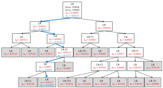
Figure 4: The locally optimal tree of predictors for ToPs/LR applied to the Bank Marketing dataset

V-D Heart Transplants

The UNOS (United Network for Organ Transplantation) dataset (available at https://www.unos.org/data/) provides information about the entire cohort of 36,329 patients (in the U.S.) who were on a waiting list to receive a heart transplant but did not receive one, during the period 1985-2015. Patients in the dataset are described by a total of 334 clinical features, but much of the feature information is missing, so we discarded 301 features for which more than 10% of the information was missing, leaving us with 33 features – 14 continuous and 19 binary. To deal with the missing information, we used 10 multiple imputations using Multiple Imputation by Chained Equations (MICE) [28]. In this setting, the objective(s) are to predict survival for time horizons of 3 months, 1 year, 3 years and 10 years. (In the dataset, 68.3% survived for 3 months, 49.5% survived for 1 year, 28.3% survived for 3 years, and 6.9% survived for 10 years.) To evaluate performance, we divided the patient data based on the admission year: we took patients admitted to a waiting list in 1985-1999 as the training sample and patients admitted in 2000-2015 as the testing sample. We compared the performance of ToPs with the same machine-learning algorithms as before; the results are shown in Table IV. Once again, both ToPs/LR and ToPs/$\mathcal{B}$ outperform all the other machine learning algorithms: ToPs/$\mathcal{B}$ achieves losses (measured as $1-AUC$) between $0.175$ and $0.207$; these improve by 17.9% to 22.3% over the best machine learning benchmarks. The improvement over Random Forest at the 3-month horizon is statistically significant (p-value = 0.012); all other improvements are highly significant (p-values $\leq$ 0.006). The Supplementary Materials show the locally optimal trees of predictors for this dataset.

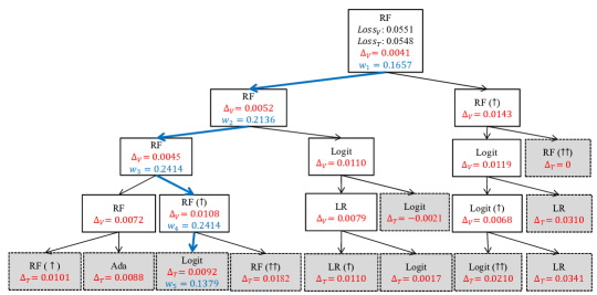
Figure 5: The locally optimal tree of predictors for ToPs/$\mathcal{B}$ applied to the Bank Marketing dataset

VI Discussion

As the experiments show, our method yields significant performance gains over a large variety of existing machine learning algorithms. These performance gains come from the concatenation of a number of different factors. To aid in the discussion, we focus on the Bank Dataset and refer to Fig. 4 and 5, which show the locally optimal trees of predictors grown by ToPs/LR and ToPs/$\mathcal{B}$, respectively. For ToPs/$\mathcal{B}$, which uses multiple learners, we show, in each node, the learner assigned to that node; for both ToPs/LR and ToPs/$\mathcal{B}$ we indicate the training set assigned to that node: For instance, in Fig. 5, Random Forest is the learner assigned to the initial node; the training set is necessarily the entire feature space $X$. In subsequent nodes, the training set is either the given node (if there is no marker) or the immediately preceding node (if the node is marked with a single up arrow) or the node preceding that (if the node is marked with two up arrows), and so forth. Note that different base learners and/or different training sets are used in various nodes. In each non-terminal node we also show the loss improvement $\Delta_{v}$ (computed with respect to $V^{1}$) obtained by splitting this node into the two immediate successor nodes. (By construction, we split exactly when improvement is possible so $\Delta_{v}$ is necessarily strictly positive at every non-terminal node while $\Delta_{v}$ would be $0$ at terminal nodes.) At the terminal nodes (shaded), we show the loss improvement $\Delta_{t}$ achieved on that node (that set of features) that is obtained by using the final predictor rather than the initial predictor. Finally, for one particular path through the tree (indicated by heavy blue arrows), we show the weights assigned to the nodes along that path in computing the overall predictor. Note that the deeper nodes do not necessarily get greater weight: using the second validation set to optimize the weights compensates for overfitting deeper in the tree.

The first key feature of our construction is that it identifies a family of subsets of the feature space – the nodes of the locally optimal tree – and optimally matches training sets to the nodes. Moreover, as Fig. 4 and 5 make clear, the optimal training set at the node $C$ need not be the node $C$ itself, but might be one of its predecessor nodes. For ToPs/LR it is this matching of training sets to nodes that gives our method its power: if we were to use the entire training set $S$ at every node, our final predictor would reduce to simple Linear Regression – but, as Table III shows, because we do match training sets to nodes, the performance of ToPs/LR is 27.1% better than that of Linear Regression.

The second key feature of our construction is that it also optimally matches learners to the nodes. For ToPs/LR, there is only a single base learner, so the matching is trivial (LR is matched to every node) – but for ToPs/$\mathcal{B}$ there are five base learners and the matching is not trivial. Indeed, as can be seen in Fig. 5, of the five available base learners, four are actually used in the locally optimal tree. This explains why ToPs/$\mathcal{B}$ improves on ToPs/LR. Of course, the performance of ToPs/$\mathcal{B}$ might be even further improved by enlarging the set of base learners. (It seems clear that the performance of ToPs/$\mathcal{A}$ depends to some extent on the set of base learners $\mathcal{A}$.)

Our recursive construction leads, in every stage, to a (potential) increase in the complexity of the predictors that can be used. For example, Linear Regression fits a linear function to the data; ToPs/LR fits a piecewise linear function to the data. This additional complexity raises the problem of overfitting. However, because we train on the training set $S$ and evaluate on the first validation set $V^{1}$, we avoid overfitting to the training set. As can be seen from Fig. 4 and 5 this avoidance of overfitting is reflected in the way it limits the depth of the locally optimal tree: the growth of the tree stops when splitting no longer yields improvement on the validation set $V^{1}$. Although training on $S$ and evaluating on $V^{1}$ avoids overfitting to $S$, it leaves open the possibility of overfitting to $V^{1}$; we avoid this problem by using the second validation set $V^{2}$ to construct optimal weights to aggregate predictions along paths.

The contrast with model trees (see again the discussion in Subsection II-A) is particular worth noting. Even ToPs/LR performs significantly better than the best model trees because we assign predictive models to every node, we construct these models by training on either the current node or some parent node, we allow for splitting when only one side of the split improves performance, and we construct the final prediction as the weighted average of predictions along the path. ToPs/$\mathcal{B}$ performs even better than ToPs/LR because we also allow for a richer family of base learners.

VII Conclusion

In this paper, we develop a new approach to ensemble learning. We construct a locally optimal tree of predictors that matches learners and training sets to particular subsets of the feature space and aggregates these individual predictors according to endogenously determined weights. Experiments on a variety of datasets show that this approach yields statistically significant improvements over state-of-the-art methods.

TABLE V: Comparison of optimization equations with existing ensemble methods

Methods	Optimization
ToPs	min_ { X_1,…,X_k } ∑_i=1^k min_h_i ∈H = ∪H_l [ 1N ∑_n=1^N L(h_i(x_j),y_j) ] ToPs uses both multiple training sets ($\{\mathcal{X}_{1},\mathcal{X}_{2},...,\mathcal{X}_{k}\}$) and multiple hypothesis classes ($\mathcal{H}=\cup\mathcal{H}_{l}$) to construct the predictive models ($\{h_{1},h_{2},...,h_{k}\}$). Both multiple training sets and corresponding predictive models are jointly optimized to minimize the loss function $\mathcal{L}$. $x_{j}$ is the $j$-th feature, $y_{j}$ is the $j$-th label, $N$ is the total number of samples, and $k$ is the number of leaves.
Bagging	min_h_i ∈H [ 1|S| ∑_(x_j,y_j) ∈S L(h_i(x_j),y_j) ] Here $S$ is the family of multiple training sets, randomly drawn. Bagging uses multiple training sets (randomly drawn) and a single hypothesis class to construct multiple predictive models. Only the predictive models are optimized to minimize the loss function $(\mathcal{L})$.
Boosting	min_h_i ∈H [ 1|S| ∑_(x_j,y_j) ∈S ϕ_j L(h_i(x_j),y_j) ] Here $S$ is the family of multiple training sets, randomly drawn. Boosting uses multiple training sets (weighted by prediction error ($\phi_{j}$) of the previous model) and a single hypothesis class to construct the predictive models. Only the predictive models are optimized to minimize the loss function ($\mathcal{L}$).
Stacking	min_h_i ∈H = ∪H_l [ 1|S| ∑_(x_j,y_j) ∈S L(h_i(x_j),y_j) ] Stacking uses a single training set with multiple hypothesis classes to construct the predictive models. Only the predictive models are optimized to minimize the loss function ($\mathcal{L}$) .

Appendix A Proof of the theorem 1 (Bounds for the predictive model of each terminal node)

Proof.

The definition of $\mathcal{R}(\mathcal{A},S)$ is

$$\mathcal{R}(\mathcal{A},S)=\frac{1}{|S|}\mathbb{E}_{\sigma=\{\pm 1\}^{|S|}}[\sup_{h\in\mathcal{A}}\sum_{z\in S}\sigma_{i}\times l(h,z_{i})]$$

where $P(\sigma_{i}=1)=P(\sigma_{i}=-1)=0.5$.
Let us define $\{{A}_{1},...,{A}_{p}\}$ as the set of all hypothesis classes that ToPs uses.
Then, let us define hypothesis class $\mathcal{A}$ as follow.

$$\mathcal{A}=\{h=\sum_{i=1}^{p}w_{i}\times h_{i}|{\bf w}\in\mbox{simplex},h_{i}\in A_{i}\}$$

Then,

$$\mathcal{R}(\mathcal{A},S) =\frac{1}{|S|}\mathbb{E}_{\sigma=\{\pm 1\}^{|S|}}[\sup_{h\in\mathcal{A}}\sum_{z\in S}\sigma_{i}\times l(h,z)]$$

$$=\frac{1}{|S|}\mathbb{E}_{\sigma=\{\pm 1\}^{|S|}}[\sup_{h\in\mathcal{A}}\sum_{z\in S}\sigma_{i}\times l(\sum_{j=1}^{p}w_{j}h_{j},z)]$$

$$=\frac{1}{|S|}\mathbb{E}_{\sigma=\{\pm 1\}^{|S|}}[\sup_{h\in\mathcal{A}}\sum_{z\in S}\sigma_{i}\times l(\sum_{j=1}^{p}w_{j}h_{j},\sum_{j=1}^{p}w_{j}z)]$$

$$=\frac{1}{|S|}\mathbb{E}_{\sigma=\{\pm 1\}^{|S|}}[\sup_{h\in\mathcal{A}}\sum_{z\in S}\sigma_{i}\times\hat{l}(\sum_{j=1}^{p}w_{j}(h_{j}-z))]$$

$$\leq\frac{1}{|S|}\mathbb{E}_{\sigma=\{\pm 1\}^{|S|}}[\sup_{h\in\mathcal{A}}\sum_{z\in S}\sigma_{i}\times\sum_{j=1}^{p}w_{j}\hat{l}(h_{j}-z)]$$

$$=\frac{1}{|S|}\mathbb{E}_{\sigma=\{\pm 1\}^{|S|}}[\sup_{h\in\mathcal{A}}\sum_{z\in S}\sigma_{i}\times\sum_{j=1}^{p}w_{j}{l}(h_{j},z)]$$

$$\leq\frac{1}{|S|}\mathbb{E}_{\sigma=\{\pm 1\}^{|S|}}[\sup_{h\in\mathcal{A}}\sum_{z\in S}\sigma_{i}\times\max_{j}l(h_{j},z)]$$

$$=\max_{j}\mathcal{R}(\mathcal{A}_{j},S)$$

Therefore, using the Rademacher Complexity Theorem,

$$\mathbb{E}_{\mathcal{D}}[L(h)] \leq L(h,S)+2\max_{i}\mathcal{R}(A_{i},S)+4\sqrt{\frac{2\log(4/\delta)}{|S|}}$$

For each terminal node $\bar{C}$, the hypothesis class is $H=\sum_{C\in\Pi(\bar{C})}w^{*}(\Pi(\bar{C}),C)\times h_{C}$. Therefore, the upper bound of the expected loss for each terminal node $\bar{C}$ is

$$\mathbb{E}_{\mathcal{D}_{\bar{C}}}[L(H)]\leq L(H,S(\bar{C}))+2\max_{C\in\Pi(\bar{C})}\mathcal{R}(A_{C},S(\bar{C}))$$

$$+4\sqrt{\frac{2\log(4/\delta)}{m}}$$

where $m=|S(\bar{C})|$. ∎

Appendix B Proof of the corollary 1.1 (Bounds for the entire predictive model)

Proof.

Based on the assumption,

$$L(h,Z)=\frac{1}{m}\sum_{z\in Z}l(h,z)$$

where $m=|Z|$. Then

$$\mathbb{E}_{\mathcal{D}}(L(H))=\sum_{\bar{C}\in\bar{T}}P(\bar{C})\times\mathbb{E}_{\mathcal{D}_{\bar{C}}}[L(H)]$$

Based on the Theorem 1, with probability at least $(1-\delta)^{1/|\bar{\mathcal{T}}|}$, each terminal node $\bar{C}$ satisfied the following condition.

$$\mathbb{E}_{\mathcal{D}_{\bar{C}}}[L(H)]\leq L(H,S(\bar{C}))+2\max_{C\in\Pi(\bar{C})}\mathcal{R}(A_{C},S(\bar{C}))$$

$$+4\sqrt{\frac{2\log(4/(1-(1-\delta)^{1/|\bar{\mathcal{T}}|}))}{m}}$$

where $m=|S(\bar{C})|$.
Because the definition of the $L(h,Z)$ is the sample mean of each loss $l(h,z)$, the entire loss is the weighted average of each terminal node. (weight is the number of samples $S(|\bar{C}|)$ in each terminal node) .
Furthermore, if each terminal node satisfies the above condition with probability at least $(1-\delta)^{1/|\bar{\mathcal{T}}|}$, it means that the probability that all terminal nodes satisfies the following condition is at least $((1-\delta)^{1/|\bar{\mathcal{T}}|})^{|\bar{\mathcal{T}}|}=(1-\delta)$
Therefore, with at least $1-\delta$ probability,

$$\mathbb{E}_{\mathcal{D}}[L(H)]\leq \sum_{\bar{C}\in\bar{T}}\frac{|S(\bar{C})|}{n}L(H,S(\bar{C}))$$

$$+2\sum_{\bar{C}\in\bar{T}}\frac{|S(\bar{C})|}{n}\max_{C\in\Pi(\bar{C})}\mathcal{R}(A_{C},S(\bar{C}))$$

$$+4\sum_{\bar{C}\in\bar{T}}\frac{|S(\bar{C})|}{n}\sqrt{\frac{2\log[4/(1-(1-\delta)^{1/|\bar{\mathcal{T}}|})]}{|S(\bar{C})|}}$$

Furthermore, $1-(1-\delta)^{1/|\bar{\mathcal{T}}|}\geq\frac{\delta}{|\bar{\mathcal{T}}|}$. Thus, we can switch $1-(1-\delta)^{1/|\bar{\mathcal{T}}|}$ to $\frac{\delta}{|\bar{\mathcal{T}}|}$ in this inequality. (Using Binomial Series Theorem, the inequality is easily proved.) Therefore, with at least $1-\delta$ probability,

$$\mathbb{E}_{\mathcal{D}}[L(H)]\leq \frac{1}{n}\sum_{\bar{C}\in\overline{{\mathcal{T}}}}|S(\bar{C})|\times$$

$$\Bigg{[}L(H,S(\overline{C}))+2\max_{C\in\Pi(\overline{C})}\,\mathcal{R}(A_{C},S(\overline{C}))$$

$$+4\sqrt{\frac{2\log(4|\bar{\mathcal{T}}|/\delta)}{|S(\overline{C})|}}\Bigg{]}$$

∎

Appendix C Proof of the computational complexity

C-A Proof of computational complexity of one recursive step:

Statement: The computational complexity of one recursive step for constructing tree of predictors grows as $\sum_{i=1}^{M}\mathcal{O}(ND\times T_{i}(N,D))$.

Proof.

There are two procedures in one recursive steps of constructing a tree of predictors. (1) Greedy search for the division point, (2) Construct the predictive model for each division.

First, the possible combinations of dividing the feature space into two subspaces using one feature with the threshold are at most $N\times D$ where $N$ is the total number of samples, and $D$ is the number of dimensions. Because, in each subspace, there should be at least one sample.

Second, for each division, we need to construct $M$ predictive models. The computational complexity to construct the $M$ number of predictive models for each division is trivially computed as $\sum_{i=1}^{M}\mathcal{O}(T_{i}(N,D))$ where $\mathcal{O}(T_{i}(N,D))$ is the computational complexity of $i$-th learner to construct the predictive model with $N$ samples and $D$ dimensional features.

Therefore, the computational complexity of one recursive step with $M$ learner can be written as follow.

$$ND\times\sum_{i=1}^{M}\mathcal{O}(T_{i}(N,D))=\sum_{i=1}^{M}\mathcal{O}(ND\times T_{i}(N,D))$$

Because, there are $ND$ possibilities of division and for each division, the computational complexity is $\sum_{i=1}^{M}\mathcal{O}(T_{i}(N,D))$.

∎

C-B Proof of computational complexity of constructing the entire tree of predictors

Statement: The computational complexity of constructing the entire tree of predictors is $\sum_{i=1}^{M}\mathcal{O}(N^{2}D\times T_{i}(N,D))$

Proof.

By the previous statement, we know that the computational complexity of one recursive step of constructing the tree of predictors is $\sum_{i=1}^{M}\mathcal{O}(ND\times T_{i}(N,D))$. Therefore, now, we need to figure out the maximum number of recursive steps with $N$ samples.

For each recursive step, the number of clusters is stepwise increased. Furthermore, in each cluster, there should be at least one sample. Therefore, we can easily figure out that the maximum number of recursive steps are at most $N$. (Note that the recursive steps are much less needed in practice because ToPs does not divide all the samples into different clusters)

Therefore, the computational complexity of the entire construction of tree of predictors is as follow.

$$N\times\sum_{i=1}^{M}\mathcal{O}(ND\times T_{i}(N,D))=\sum_{i=1}^{M}\mathcal{O}(N^{2}D\times T_{i}(N,D))$$

∎

For instance, if we only use the linear regression as the learner of ToPs (ToPs/LR), the computational complexity of ToPs is $\mathcal{O}(N^{3}D^{3})$. This is because, the computational complexity of linear regression is $\mathcal{O}(ND^{2})$. Therefore, the entire computational complexity of ToPs/LR is $\sum_{i=1}^{M}\mathcal{O}(N^{2}DT_{i}(n,D))=\mathcal{O}(N^{3}D^{3})$

References

- [1] D. J. Miller and L. Yan, “Critic-driven ensemble classification,” IEEE Transactions on Signal Processing, vol. 47, no. 10, pp. 2833–2844, 1999.
- [2] C. Tekin, J. Yoon, and M. van der Schaar, “Adaptive ensemble learning with confidence bounds,” IEEE Transactions on Signal Processing, vol. 65, no. 4, pp. 888–903, 2016.
- [3] N. Asadi, A. Mirzaei, and E. Haghshenas, “Multiple observations hmm learning by aggregating ensemble models,” IEEE Transactions on Signal Processing, vol. 61, no. 22, pp. 5767–5776, 2013.
- [4] L. Canzian, Y. Zhang, and M. van der Schaar, “Ensemble of distributed learners for online classification of dynamic data streams,” IEEE Transactions on Signal and Information Processing over Networks, vol. 1, no. 3, pp. 180–194, 2015.
- [5] L. Breiman, “Random forests,” Machine learning, vol. 45, no. 1, pp. 5–32, 2001.
- [6] Y. Freund, Y. Mansour, and R. E. Schapire, “Generalization bounds for averaged classifiers,” Annals of Statistics, pp. 1698–1722, 2004.
- [7] D. J. MacKay, “Bayesian methods for adaptive models,” Ph.D. dissertation, California Institute of Technology, 1992.
- [8] V. Y. Tan, S. Sanghavi, J. W. Fisher, and A. S. Willsky, “Learning graphical models for hypothesis testing and classification,” IEEE Transactions on Signal Processing, vol. 58, no. 11, pp. 5481–5495, 2010.
- [9] Y. Freund and R. E. Schapire, “A decision-theoretic generalization of on-line learning and an application to boosting,” in European conference on computational learning theory. Springer, 1995, pp. 23–37.
- [10] P. Smyth and D. Wolpert, “Linearly combining density estimators via stacking,” Machine Learning, vol. 36, no. 1-2, pp. 59–83, 1999.
- [11] J. R. Quinlan et al., “Learning with continuous classes,” in 5th Australian joint conference on artificial intelligence, vol. 92. Singapore, 1992, pp. 343–348.
- [12] Y. Wang and I. H. Witten, “Induction of model trees for predicting continuous classes,” 1996.
- [13] L. Torgo, “Functional models for regression tree leaves,” in ICML, vol. 97. Citeseer, 1997, pp. 385–393.
- [14] D. Potts and C. Sammut, “Incremental learning of linear model trees,” Machine Learning, vol. 61, no. 1-3, pp. 5–48, 2005.
- [15] D. Malerba, F. Esposito, M. Ceci, and A. Appice, “Top-down induction of model trees with regression and splitting nodes,” IEEE Transactions on Pattern Analysis and Machine Intelligence, vol. 26, no. 5, pp. 612–625, 2004.
- [16] L. Breiman, J. Friedman, C. J. Stone, and R. A. Olshen, Classification and regression trees. CRC press, 1984.
- [17] L. Breiman, “Bagging predictors,” Machine learning, vol. 24, no. 2, pp. 123–140, 1996.
- [18] C. Cortes, M. Mohri, and U. Syed, “Deep boosting,” in 31st International Conference on Machine Learning, ICML 2014. International Machine Learning Society (IMLS), 2014.
- [19] J. Friedman, T. Hastie, R. Tibshirani et al., “Additive logistic regression: a statistical view of boosting (with discussion and a rejoinder by the authors),” The annals of statistics, vol. 28, no. 2, pp. 337–407, 2000.
- [20] T. Chen and C. Guestrin, “Xgboost: A scalable tree boosting system,” in Proceedings of the 22Nd ACM SIGKDD International Conference on Knowledge Discovery and Data Mining. ACM, 2016, pp. 785–794.
- [21] P. Smyth and D. Wolpert, “Linearly combining density estimators via stacking,” Machine Learning, vol. 36, no. 1-2, pp. 59–83, 1999.
- [22] E. A. Nadaraya, “On estimating regression,” Theory of Probability & Its Applications, vol. 9, no. 1, pp. 141–142, 1964.
- [23] G. S. Watson, “Smooth regression analysis,” Sankhyā: The Indian Journal of Statistics, Series A, pp. 359–372, 1964.
- [24] C. K. Williams, “Prediction with gaussian processes: From linear regression to linear prediction and beyond,” in Learning in graphical models. Springer, 1998, pp. 599–621.
- [25] Y. LeCun, “The mnist database,” 2016. [Online]. Available: http://yann.lecun.com/exdb/mnist/
- [26] M. Lichman, “UCI machine learning repository,” 2013. [Online]. Available: http://archive.ics.uci.edu/ml
- [27] S. Fritsch, F. Guenther, and M. F. Guenther, “Package ‘neuralnet’,” 2016.
- [28] S. Buuren and K. Groothuis-Oudshoorn, “mice: Multivariate imputation by chained equations in r,” Journal of statistical software, vol. 45, no. 3, 2011.