Solver composition across the PDE/linear algebra barrier

Abstract

The efficient solution of discretisations of coupled systems of partial differential equations (PDEs) is at the core of much of numerical simulation. Significant effort has been expended on scalable algorithms to precondition Krylov iterations for the linear systems that arise. With few exceptions, the reported numerical implementation of such solution strategies is specific to a particular model setup, and intimately ties the solver strategy to the discretisation and PDE, especially when the preconditioner requires auxiliary operators. In this paper, we present recent improvements in the Firedrake finite element library that allow for straightforward development of the building blocks of extensible, composable preconditioners that decouple the solver from the model formulation. Our implementation extends the algebraic composability of linear solvers offered by the PETSc library by augmenting operators, and hence preconditioners, with the ability to provide any necessary auxiliary operators. Rather than specifying up front the full solver configuration, tied to the model, solvers can be developed independently of model formulation and configured at runtime. We illustrate with examples from incompressible fluids and temperature-driven convection.

65N22, 65F08, 65F10

1 Introduction

For over a decade now, domain-specific languages for numerical partial differential equations (henceforth PDEs) such as Sundance [30, 29], FEniCS [28], and now Firedrake [40] have enabled users to efficiently generate algebraic systems from a high-level description of the variational problems. Both FEniCS and Firedrake make use of the Unified Form Language [1] as a description language for the weak forms of PDEs, converting it into efficient low-level code for form evaluation. They also share a Python interface that, for the intersection of their feature sets, is nearly source-compatible. These high-level PDE codes succeed by connecting a rich description language for PDEs to effective lower-level solver libraries such as PETSc [4, 5] or Trilinos [21] for the requisite, and performance-critical, numerical (non)linear algebra.

These high-level PDE projects utilise the solver packages in an essentially unidirectional way: the residuals are evaluated, Jacobians formed, and are then handed off to mainly algebraic techniques. Hence, the codes work at their best when (compositions of) existing black-box matrix techniques effectively solve the algebraic systems. However, in many situations the best preconditioners require additional structure beyond a purely algebraic (matrix and vector-level) problem description. Many of the preconditioners for block systems based on block factorisations require discretisations of differential operators not contained in the original problem. These include the pressure-convection-diffusion (PCD) approximation for Navier-Stokes [25, 16], and preconditioners for models of phase separation [19, 24]. An alternate approach to derive preconditioners for block systems is to use arguments from functional analysis to arrive at block-diagonal preconditioners. While these are often representable as the inverse of an assembled operator, in some cases, a mesh and parameter independent preconditioner that arises from such an analysis requires the action of the sum of inverses. An example is the preconditioner suggested in [32, example 4.2] for the time-dependent Stokes problem.

While a high-level PDE engine makes it possible to obtain these new operators at low user cost, additional care is required to develop a clean, extensible interface. For example, the PCD preconditioner has been implemented using Sundance and Playa [23], although the resulting code tightly fused the description of the problem with a highly specialised specification of the preconditioner. Similarly, in the FEniCS project, cbc.block [31] allows the model developer to write complex block preconditioners as a composition of high-level “symbolic” linear algebra operations; Trilinos provides similar functionality through Teko [12]. However, in these codes one must specify up front how to perform the block decomposition. Switching to a different preconditioner requires changing the model code, and there is no high-level manipulation of variational problems within the blocks. Ideally, one would like a mechanism to implement the specialised preconditioner as a separate component, leaving the original application code essentially unchanged.

Extensibility of fundamental types such as solvers, preconditioners, and matrices has long been a main concern of the PETSc project. For example, the action of a finite difference stencil applied to a vector can be wrapped behind a matrix “shell” interface and used interchangeably with explicit sparse matrices for many purposes. Users can similarly provide custom types of Krylov methods or preconditioners. Thanks to petsc4py [13], such extensions can be implemented in Python as well as C. Moreover, PETSc provides powerful tools to switch between (compositions of) existing and custom tools either in the application source code or through command-line options.

In this work, we enable the rapid development of high-performance preconditioners as PETSc extensions using Firedrake and petsc4py. To facilitate this, we have developed a custom matrix type that embeds the complete Firedrake problem description (UFL variational forms, function spaces, meshes, etc) in a Python context accessible to PETSc. As a happy byproduct, this enables low-memory matrix-free evaluation of matrix-vector products. This also allows us to produce PETSc preconditioners in petsc4py that act on this new matrix type, accessing the PDE-level information as needed. For example, a PCD preconditioner can access the meshes and function spaces to create bilinear forms for, and hence assemble, the needed mass, stiffness, and convection-diffusion operators on the pressure space along with PETSc KSP (linear solver) contexts for the inverses. Moreover, once such preconditioners are available in a globally importable module, it is now possible to use them instead of existing algebraic preconditioners by a straightforward runtime modification of solver configuration options. So, we use our PDE language not only to generate problems to feed to the solver, but also to extend that solver’s capabilities.

Our discussion and implementation will focus on Firedrake as the top-level PDE library and PETSc as the solver library. Firedrake already relies heavily on PETSc through petsc4py and has a nearly pure Python implementation. Provided one is content with the Python interface, it should not be terribly difficult to adapt these techniques for use in FEniCS. Regarding solver libraries, the idiom and usage of Trilinos and PETSc (if not their actual capabilities) differ considerably, so we make no speculation as to the difficulties associated with adapting our techniques in that direction.

In the rest of the paper, we set up certain model problems in Section 2. After this, in Section 3 we survey certain algorithms that go beyond the current mode of algebraically preconditioning assembled matrices. These include matrix-free methods, Schwarz-type preconditioners, and preconditioners that require auxiliary differential operators. It turns out that a proper implementation of the first of these, matrix-free methods, provides a very clean way to communicate PDE-level problem information between PETSc matrices and custom preconditioners, and we describe the implementation of this and relevant modifications to Firedrake in Section 4. Finally, we give examples demonstrating the efficacy of our approach to the model problems of interest in Section 5.

2 Some model applications

2.1 The Poisson equation

It is helpful to fix some target applications and describe things we would like to expedite within our top-level code.

A usual starting point is to consider a second-order scalar elliptic equation. Let $\Omega\subset\mathbb{R}^{d}$, where $d=1,2,3$, be a domain with boundary $\Gamma$. We let $\kappa:\Omega\rightarrow\mathbb{R}^{+}$ be some positive-valued coefficient. On the interior of $\Omega$, we seek a function $u$ satisfying

(1) $$-\nabla\cdot\left(\kappa\nabla u\right)=f$$

subject to the boundary condition $u=u_{\Gamma_{D}}$ on $\Gamma_{D}$ and $\nabla u\cdot n=g$ on $\Gamma_{N}$.

After the usual technique of multiplying by a test function and integrating by parts, we reach the weak form of seeking $u\in V_{\Gamma}\subset V$ such that

(2) $$\left(\kappa\nabla u,\nabla v\right)=\left(f,v\right)-\left\langle g,\frac{\partial v}{\partial n}\right\rangle$$

for all $v\in V_{0}\subset V$, where $V$ is the finite element space, $V_{0}$ the subspace with vanishing trace on $\Gamma_{D}$. Here $(\cdot,\cdot)$ denotes the standard $L^{2}$ inner product over $\Omega$, and $\langle\cdot,\cdot\rangle$ that over $\Gamma$.

The finite element method leads to a linear system:

(3) $$Au=f,$$

where $A$ is symmetric and positive-definite (positive semi-definite if $\Gamma_{D}=\varnothing$), and the vector $f$ includes both the forcing term and contributions from the boundary conditions.

2.2 The Navier-Stokes equations

Moving beyond the simple Poisson operator, the incompressible Navier-Stokes equations provide additional challenges.

(4a) $$-\frac{1}{\text{Re}}\Delta\mathbf{u}+\mathbf{u}\cdot\nabla\mathbf{u}+\nabla p =0,$$

(4b) $$\nabla\cdot\mathbf{u} =0$$

together with suitable boundary conditions.

Among the diverse possible methods, we shall focus here on inf-sup stable mixed finite element spaces such as Taylor-Hood [9]. This is merely for simplicity of explication and does not represent a limitation of our approach or implementation. Taking $V_{\Gamma}$ to be subset of the discrete velocity space satisfying any strongly imposed boundary conditions and $W$ the pressure space, we have the weak form of seeking $\mathbf{u},p$ in $V_{\Gamma}\times W$ such that

(5a) $$\frac{1}{\text{Re}}\left(\nabla\mathbf{u},\nabla\mathbf{v}\right)+\left(\mathbf{u}\cdot\nabla\mathbf{u},\mathbf{v}\right)-\left(p,\nabla\cdot\mathbf{v}\right) =0,$$

(5b) $$\left(\nabla\cdot\mathbf{u},w\right) =0$$

for all $\mathbf{v},w\in V_{0}\times W$, where $V_{0}$ is the velocity subspace with vanishing Dirichlet boundary conditions.

Relative to the Poisson equation, we now have several additional challenges. The nonlinearity may be addressed by Newton linearisation, and UFL provides automatic differentiation to produce the Jacobian. We also have multiple finite element spaces, one of which is vector-valued. Further, for each nonlinear iteration, the required linear system is larger and more complicated, a block-structured saddle point system of the form

(6) $$\begin{bmatrix}F&-B^{t}\\ B&0\end{bmatrix}\begin{bmatrix}\mathbf{u}\\ p\end{bmatrix}=\begin{bmatrix}f_{1}\\ f_{2}\end{bmatrix}.$$

Black-box algebraic preconditioners tend to perform poorly here, and we discuss some more effective alternatives in Section 3.

2.3 Rayleigh-Bénard convection

Many applications rely on coupling other processes to the Navier-Stokes equations. For example, Rayleigh-Bénard convection [11] includes thermal variation in the fluid, although we take the Boussinesq approximation that temperature variations affect the momentum balance only as a buoyant force. We have, after nondimensionalisation,

(7a) $$-\Delta\mathbf{u}+\mathbf{u}\cdot\nabla\mathbf{u}+\nabla p =-\frac{\text{Ra}}{\text{Pr}}Tg\hat{\mathbf{z}},$$

(7b) $$\nabla\cdot\mathbf{u} =0,$$

(7c) $$-\text{Pr}\Delta T+\mathbf{u}\cdot\nabla T =0,$$

where Ra is the Rayleigh number, Pr is the Prandtl number, $g$ is the acceleration due to gravity, and $\hat{\mathbf{z}}$ the upward-pointing unit vector. The problem is usually posed on rectangular domains, with no-slip boundary conditions on the fluid velocity. The temperature boundary conditions typically involve imposing a unit temperature difference in one direction with insulating boundary conditions in the others.

After discretisation and Newton linearisation, one obtains a block $3\times 3$ system

(8) $$\begin{bmatrix}F&-B^{t}&M_{1}\\ B&0&0\\ M_{2}&0&K\end{bmatrix}\begin{bmatrix}\mathbf{u}\\ p\\ T\end{bmatrix}=\begin{bmatrix}f_{1}\\ f_{2}\\ f_{3}\end{bmatrix}.$$

Here, the $F$ and $B$ matrices are as obtained in the Navier-Stokes equations (with $\text{Re}=1$). The $M_{1}$ and $M_{2}$ terms arise from the temperature/velocity coupling, and $K$ is the convection-diffusion operator for temperature.

Alternately, letting

(9a) $$N =\begin{bmatrix}F&-B^{t}\\ B&0\end{bmatrix},$$

(9b) $$\widetilde{M}_{1} =\begin{bmatrix}M_{1}\\ 0\end{bmatrix},$$

(9c) $$\widetilde{M}_{2} =\begin{bmatrix}M_{2}&0\end{bmatrix},$$

we can write the stiffness matrix as block $2\times 2$ matrix

(10) $$\begin{bmatrix}N&\widetilde{M}_{1}\\ \widetilde{M}_{2}&K\end{bmatrix}.$$

Formulating the matrix in this way allows us to consider composing some (possibly custom) solver technique for Navier-Stokes with other approaches to handle the temperature equation and coupling.

3 Solution techniques

Via UFL, Firedrake has a succinct, high-level description of these equations and can readily linearise and assemble discrete operators. When efficient techniques for the discrete system exist within PETSc, obtaining the solution is as simple as providing the proper options. When direct methods are applicable, simple options like -ksp_type preonly -pc_type lu suffice – possibly augmented with the selection of a package to perform the factorisation like MUMPS [2] or UMFPACK [14]. Similarly, when iterative methods with black-box preconditioners such as incomplete factorisation or algebraic multigrid fit the bill, options such as -ksp_type cg -pc_type hypre work. PETSc also provides many block preconditioner mechanisms via FieldSplit, allowing users to specify PETSc solvers for inverting the relevant blocks [10]. Firedrake automatically enables this by specifying index sets for each function space, passing the information to PETSc when it initialises the solver. A key feature of PETSc is that these choices can be made at runtime via options, without modifying the user code that specifies the PDE to solve.

As we stated in the introduction, however, many techniques for preconditioning require information beyond what can be learned by an inspection of matrix entries and user-specified options. It is our goal now to survey some of these techniques in more detail, after which we describe our implementation of custom PETSc preconditioners to utilise application-specific problem descriptions in a clean, efficient, and user-friendly way.

3.1 Matrix-free methods

Switching from a low order method to a higher-order one simply requires changing a parameter in the top-level Firedrake application code. However, such a small change can profoundly affect the overall performance footprint. Assembly of stiffness matrices becomes more expensive, both in terms of time and space, as the order increases. An alternative, that does not have the same constraints is to use a matrix-free implementation of the matrix-vector product. This is sufficient for Krylov methods, although not for algebraic preconditioners requiring matrix entries.

Rather than producing a sparse matrix $A$, one provides a function that, given a vector $x$, computes the product $Ax$. Abstractly, consider a bilinear form $a$ on a discrete space $V$ with basis $\{\psi_{i}\}_{i=1}^{N}$. The $N\times N$ stiffness matrix $A_{ij}=a(\psi_{j},\psi_{i})$ can be applied to a vector $x$ as follows. Any vector $x$ is isomorphic to some function $u\in V$ via the identification $x\leftrightarrow u=\sum_{j=1}^{N}x_{j}\psi_{j}$. Then, via linearity,

(11) $$\begin{split}\left(Ax\right)_{i}&=\sum_{j=1}^{N}A_{ij}x_{j}=\sum_{j=1}^{N}a(\psi_{i},\psi_{j})x_{j}\\ &=a(\psi_{i},\sum_{j=1}^{N}x_{j}\psi_{j})=a(\psi_{i},u).\end{split}$$

Just like matrices or load vectors, this can be computed by assembling elementwise contributions in the standard way, considering $u$ to be just some given member of $V$.

In the presence of strongly-enforced boundary conditions, the bilinear form acts on a subspace $V_{0}\subset V$. When a matrix is explicitly assembled, one typically either edits (or removes) rows and columns to incorporate the boundary conditions. Care must be taken in enforcing the boundary conditions to ensure that the matrix-free action agrees with multiplication by the matrix that would have been assembled.

Typically, such an approach has a much lower startup cost than an explicit sparse matrix since no assembly is required. Forgoing an assembled matrix also saves considerably on memory usage. Moreover, the arithmetic intensity ($\operatorname{ai}$) of matrix-free operator application is almost always higher than that of an assembled matrix (sparse matrix multiplication has $\operatorname{ai}\approx 1/6\operatorname{flop}/\operatorname{byte}$ [20]). Matrix-free methods are therefore an increasingly good match to modern memory bandwidth-starved hardware, where the balanced arithmetic intensity is $\operatorname{ai}\approx 10$. The algorithmic complexity is either the same ($\mathcal{O}(p^{2d})$ for degree $p$ elements in $d$ dimensions), or better ($\mathcal{O}(p^{d+1})$) if a structured basis can be exploited through sum factorisation. On simplex elements, the latter optimisation is not currently available through the form compiler in Firedrake. Thus we will expect our matrix-free operator applications to have the same algorithmic scaling as assembled matrices (though with different constant factors). If we can exploit the vector units in modern processors effectively, we can expect that matrix-free applications will be at least competitive with, and often faster than, assembled matrices (for example [33] demonstrate significant benefits, relative to assembled matrices, for $Q_{2}$ operator application on hexahedra).

3.2 Preconditioning high-order discretisations: additive Schwarz

Matrix-free methods preclude algebraic preconditioners such as incomplete factorisation or algebraic multigrid. Depending on the available smoothers, if a mesh hierarchy is available, geometric multigrid is a possibility [7, 8]. Here, we discuss a family of additive Schwarz methods. Originally proposed by Pavarino in [37, 38], these methods fall within the broad family of subspace correction methods [44].

These two-level methods decompose the finite element space into a low order space on the original mesh and the high-order space restricted to local pieces of the mesh, such as patches of cells around each vertex. Any member of the original finite element space can be written as a combination of items from this collection of subspaces, although the decomposition in this case is certainly not orthogonal. One obtains a preconditioner for the original finite element operator by additively combining the (possibly approximate) inverses of the restrictions of the original operator to these spaces. Schöberl [42] showed for the symmetric coercive case that the preconditioned system has eigenvalue bounds independent of both mesh size and polynomial degree and gave computational examples from elasticity confirming the theory. Although not covered by Schöberl’s analysis, these methods have also been applied with success to the Navier-Stokes equations [39].

This approach is generic in that it can be attempted for any problem. Given a bilinear form over a function space of degree $k$, one can programmatically build the lowest-order instance of the function space and set up the vertex patches for the mesh. Then, one can easily modify the bilinear form to operate on the new subspaces and perform the subspace correction. We have developed such a generic implementation, parametrised over the UFL problem description.

One drawback of this method is the relatively high memory cost of storing the patch-wise Cholesky or LU factors, especially at high order and in 3D. One may further decompose the local patch spaces through “spider vertices” to reduce the memory required and still retain a powerful method [42]. Such refinements are possible within our software framework, although we have not pursued them to date.

3.3 Block preconditioners and Schur complement approximations

Having motivated matrix-free methods and preconditioners for higher-order discretisations in the simple case of the Poisson operator, we now return to the Navier-Stokes equations introduced earlier. In particular, we are interested in preconditioners for the Jacobian stiffness matrix Eq. 6.

Block factorisation of the system matrix provides a starting point for many powerful preconditioners [6, 16, 18]. Consider the block LDU factorisation of the system matrix in Eq. 6 as

(12) $$\begin{bmatrix}F&-B^{t}\\ B&0\end{bmatrix}=\begin{bmatrix}I&0\\ BF^{-1}&I\end{bmatrix}\begin{bmatrix}F&0\\ 0&S\end{bmatrix}\begin{bmatrix}I&-F^{-1}B^{t}\\ 0&I\end{bmatrix},$$

where $I$ is the identity matrix of the proper size and $S=BF^{-1}B^{t}$ is the Schur complement. The inverse of this matrix is then given by

(13) $$\begin{bmatrix}F&-B^{t}\\ B&0\end{bmatrix}^{-1}=\begin{bmatrix}I&F^{-1}B^{t}\\ 0&I\end{bmatrix}\begin{bmatrix}F^{-1}&0\\ 0&S^{-1}\end{bmatrix}\begin{bmatrix}I&0\\ -BF^{-1}&I\end{bmatrix}.$$

Since this is the exact inverse, applying it in a preconditioning phase leads to Krylov convergence in a single iteration if all blocks are inverted exactly. Note that inverting the Schur complement matrix $S$ either requires assembling it as a dense matrix or else using a Krylov method where the matrix action is computed implicitly via two matrix-vector products and an inner solve to produce $F^{-1}$.

Two kinds of approximations lead to more practical methods. For one, it is possible to neglect either or both of the triangular factors. This gives a structurally simpler preconditioner, at the cost (assuming exact inversion of $S$) of a slight increase in the iteration count. For example, it is common to use only the lower triangular part of the matrix, giving a preconditioning matrix of the form

(14) $$P=\begin{bmatrix}F&0\\ B&S\end{bmatrix}$$

which has inverse

(15) $$P^{-1}=\begin{bmatrix}F^{-1}&0\\ 0&S^{-1}\end{bmatrix}\begin{bmatrix}I&0\\ -BF^{-1}&I\end{bmatrix}.$$

Using $P$ as a left preconditioner, $P^{-1}A$ is readily seen to give a unit upper triangular matrix, and it is known that GMRES will converge in two (very expensive) iterations since the resulting preconditioned matrix system has a quadratic minimal polynomial [36].

Given the cost of inverting $S$, it is also desirable to devise a suitable approximation. A simple approach is to use a pressure mass matrix, which gives mesh-independent but rather large eigenvalue bounds [17]. More sophisticated approximations are well-documented in the literature [16]. For our purposes, we will consider one in particular, the pressure convection-diffusion (hence PCD) preconditioner [15, 25]. It is based on the approximation

(16) $$S^{-1}=\left(BF^{-1}B^{t}\right)^{-1}\approx K_{p}^{-1}F_{p}M^{-1}_{p}\equiv X^{-1},$$

where $K_{p}$ is the Laplace operator acting on the pressure space, $M_{p}$ is the mass matrix, and $F_{p}$ is a discretisation of the convection-diffusion operator

(17) $$\mathcal{L}p\equiv-\frac{1}{Re}\Delta p+\mathbf{u_{0}}\cdot\nabla p,$$

with $\mathbf{u_{0}}$ the velocity at the current Newton iterate. Although this requires solving linear systems, the mass and stiffness matrices are far cheaper to invert than $F$.

While one could use this approximation to precondition a Krylov solver for $S$, it is far more typical to replace $S^{-1}$ with $X^{-1}$. For example, using the triangular preconditioner Eq. 14 gives the further approximation in a block preconditioner:

(18) $$\widetilde{P}^{-1}=\begin{bmatrix}F^{-1}&0\\ 0&X^{-1}\end{bmatrix}\begin{bmatrix}I&0\\ -BF^{-1}&I\end{bmatrix}=\begin{bmatrix}F^{-1}&0\\ 0&K_{p}^{-1}F_{p}M_{p}^{-1}\end{bmatrix}\begin{bmatrix}I&0\\ -BF^{-1}&I\end{bmatrix}.$$

Although bypassing the solution of the Schur complement system increases the outer iteration count, it typically results in a much more efficient overall method. We note that strong statements about the exact convergence in the presence of approximate inverses are rather delicate, and refer the reader to [6, §9.2, and §10] for an overview of convergence results for such problems. Also, note that only the action of the off-diagonal blocks is required for the preconditioner so that a matrix-free treatment is appropriate.

Preconditioning strategies for the Navier-Stokes equations can quickly find their way into problems coupling other processes to fluids. We return now to the Bénard convection stiffness matrix Eq. 10, where $N$ is itself the Navier-Stokes stiffness matrix in Eq. 6. Block preconditioners based on this formulation, replacing $N^{-1}$ with a very inexact solve via PCD-preconditioned GMRES, proved more effective than techniques based on $3\times 3$ preconditioners [22]. Here, we present a lower-triangular block preconditioner rather than the upper-triangular one in [22] with similar practical results.

A block Gauss-Seidel preconditioner for Eq. 10 can be taken as

(19) $$P=\begin{bmatrix}N&0\\ \widetilde{M}_{2}&K\end{bmatrix},$$

the inverse of which requires evaluation of $N^{-1}$ and $K^{-1}$:

(20) $$P^{-1}=\begin{bmatrix}N^{-1}&0\\ 0&I\end{bmatrix}\begin{bmatrix}I&0\\ -\widetilde{M}_{2}&I\end{bmatrix}\begin{bmatrix}I&0\\ 0&K^{-1}\end{bmatrix}.$$

Replacing these inverses with approximations/preconditioners $\widetilde{N}^{-1}$ and $\widetilde{K}^{-1}$ gives

(21) $$\widetilde{P}^{-1}=\begin{bmatrix}\widetilde{N}^{-1}&0\\ 0&I\end{bmatrix}\begin{bmatrix}I&0\\ -\widetilde{M}_{2}&I\end{bmatrix}\begin{bmatrix}I&0\\ 0&\widetilde{K}^{-1}\end{bmatrix}.$$

At this point, replacing $\widetilde{N}^{-1}$ with the block preconditioner Eq. 18 recovers a block lower-triangular $3\times 3$ preconditioner:

(22) $$\widetilde{P}^{-1}=\begin{bmatrix}F^{-1}&0&0\\ 0&K_{p}^{-1}F_{p}M_{p}^{-1}&0\\ 0&0&I\end{bmatrix}\begin{bmatrix}I&0&0\\ -BF^{-1}&I&0\\ 0&0&I\end{bmatrix}\begin{bmatrix}I&0&0\\ 0&I&0\\ -M_{2}&0&I\end{bmatrix}\begin{bmatrix}I&0&0\\ 0&I&0\\ 0&0&\widetilde{K}^{-1}\end{bmatrix}.$$

4 Implementation

The core object in our implementation is an appropriately designed “implicit” matrix that provides matrix-vector actions and also makes PDE-level discretisation information available to custom preconditioners within PETSc. Here, we describe this class, how it interacts with both Firedrake and PETSc, and how it provides the requisite functionality. Then, we demonstrate how it cleanly provides the proper information for custom preconditioners.

4.1 Implicit matrices

First, we note that Firedrake deals with matrices at two different levels. A Firedrake-level Matrix instance maintains symbolic information (the bilinear form, boundary conditions). It in turn contains a PETSc Mat (typically in some sparse format), which is used when creating solvers.

Our implicit matrices mimic this structure, adding an ImplicitMatrix sibling class to the existing Matrix, lifting shared features into a common MatrixBase class. Where the ImplicitMatrix differs is that its PETSc Mat now has type python (rather than a normal sparse format such as aij). To provide the appropriate matrix-vector actions, the ImplicitMatrix instance provides an ImplicitMatrixContext instance to the PETSc Mat. This context object contains the PDE-level information – the bilinear form and boundary conditions – necessary to implement matrix-vector products. Moreover, this context object enables building custom preconditioners since it is available from within the “low-level” PETSc Mat.

UFL’s adjoint function, which reverses the test and trial function in a bilinear form, also makes it straightforward to provide the action of the matrix transpose, needed in some Krylov methods [41, §7.1]. The implicit matrix constructor simply stashes the action of the original bilinear form and its adjoint, and the multiplication and transposed multiplication are nearly identical using Firedrake’s assemble method with boundary conditions appropriately enforced.

We enable FieldSplit preconditioners on implicit matrices by means of overloading submatrix extraction. The PETSc interface to submatrix extraction does not presuppose any particular block structure. Instead, the function receives integer index sets corresponding to rows and columns to be extracted into the submatrix. Since the PDE-level description operates at the level of fields, we only support extraction of submatrices that correspond to some subset of the fields that the matrix contains. Our method determines whether a provided index set is a concatenation of a subset of the index sets defining the different fields and returns the list of integer labels of the fields in the subset. While this implementation compares index sets by value and therefore increases in expense as the number of per-process degrees of freedom increases, it must only be carried out once per solve (be it linear or non-linear), since the index set structure does not change. We have not found it to be a measureable fraction of the solution time in our implementation.

Splitting implicit matrices offers an efficient alternative to splitting assembled sparse matrices. Currently, splitting a standard assembled matrix into blocks requires the allocation and copying of the subblocks. While PETSc also includes a “nested” matrix type (essentially an array of pointers to matrices), collecting multiple fields into a single block (e.g. the pressure and velocity in Bénard convection) requires that the user code state up front the order in which nesting occurs. This would mean that editing/recompilation of the code is necessary to switch between preconditioning approaches that use different variable splittings, contrary to our goal of efficient high-level solver configuration and customisation.

The typical user interface in Firedrake involves interacting with PETSc via a VariationalSolver, which takes charge of configuring and calling the PETSc linear and nonlinear solvers. It allocates matrices and sets the relevant callback functions for Jacobian and residual evaluation to be used inside SNES (PETSc’s nonlinear solver object). Switching between implicit and standard sparse matrices is now facilitated through additional PETSc database options, so that the type of Jacobian matrix is set with -mat_type and the, possibly different, preconditioner matrix type with -pmat_type. This latter option facilitates using assembled matrices for the matrix-vector product, while still providing PDE-level information to the solver. In this way, enabling matrix-free methods simply requires an options change in Firedrake and no other user modification.

4.2 Preconditioners

It is helpful to briefly review certain aspects of the PETSc formalism for preconditioners. One can think of (left) preconditioning as converting a linear system

(23) $$b-Ax=0$$

into an equivalent system

(24) $$\hat{P}\left(b-Ax\right)=0,$$

where $\hat{P}(\cdot)$ applies an approximation of the inverse of the preconditioning matrix $P$ to the residual.

Then, given a current iterate $x_{i}$, we have the residual

(25) $$r_{i}=b-Ax_{i}.$$

PETSc preconditioners are specified to act on residuals, so that $\hat{P}(r_{i})$ then gives an approximation to the error $e_{i}=x-x_{i}$. This enables sparse direct methods to act as preconditioners, converting the residual into the exact (up to roundoff error) residual, and direct solvers nonetheless conform to the KSP interface (e.g. -ksp_type preonly -pc_type lu).

PETSc preconditioners are built in terms of both the system matrix $A$ and a possibly different “preconditioning matrix” $A_{p}$ (for example, preconditioning a convection-diffusion operator with the Laplace operator). So then, $\hat{P}=\hat{P}(A,A_{p})$ is a method for constructing an (approximation to) the inverse of $A$. Preconditioner implementations must provide PETSc with an apply method that computes $y\leftarrow\hat{P}x$. Creation of the data (for example, an incomplete factorisation) necessary to apply the preconditioner is carried out in a setUp method.

Firedrake now provides Python-level scaffolding to expedite the implementation of preconditioners that act on implicit matrices. Instead of manipulating matrix entries like ILU or algebraic multigrid, these preconditioners use the UFL problem description from the Python context contained in the incoming matrix $P$ to do what is needed. Hence, these preconditioners can be parametrised not over particular matrices, but over bilinear forms. To demonstrate the generality of our approach, we have implemented several such examples.

4.2.1 Assembled preconditioners

While one can readily define block preconditioners using implicit matrices, the best methods for inverting the diagonal blocks may in fact be algebraic. This illustrates a critical use case of our simplest preconditioner acting on implicit matrices. We have defined a generic preconditioner AssembledPC whose setUp method simply forces the assembly of an underlying bilinear form and then sets up a sub-preconditioner (typically an algebraic one) acting on the sparse matrix. Then, the apply method simply forwards to that of the sub-preconditioner. For example, to use an implicit matrix-vector product but incomplete factorisation on an assembled matrix for the preconditioner, one might use options like

⬇

-mat_type matfree

-pc_type python

-pc_python_type firedrake.AssembledPC

-assembled_pc_type ilu

As mentioned, FieldSplit preconditioners provide a critical use case, enabling one to leave the overall matrix implicit, and assemble only those blocks that are required. In particular, the off-diagonal blocks never require assembly, and this can result in significant memory savings.

4.2.2 Schur complement approximations

Our next example, Schur complement approximations, is more specialised but very relevant to the problems in fluid mechanics expressed above. PETSc provides two pathways to define preconditioners for the Schur complement, such as Eq. 16. Within the source code, one may pass to the function PCFieldSplitSetSchurPre a matrix which will be used by a preconditioner to construct an approximation to the Schur complement. Alternatively, PETSc can automatically construct some approximations that may be obtained by algebraic manipulations of the original operator (such as the SIMPLE or LSC approximations [16]). While the latter may be configured using only runtime options, the former requires that the user pick apart the solver and call PCFieldSplitSetSchurPre on the appropriate PC object. Enabling this preconditioning option, or incorporating it into larger coupled systems requires modification of the model source code.

Since our implicit matrices and their subblocks contain the UFL problem specification, a preconditioner acting on the Schur complementment block has complete freedom to utilise the UFL bilinear form to set up auxiliary operators. We have implemented two Schur complement approximations suitable for incompressible flow, an inverse mass matrix and the PCD preconditioner, both of which follow a similar pattern. The setUp function extracts the pressure function space from the UFL bilinear form and defines and assembles bilinear forms for the auxiliary operators. It also defines user-configurable KSP contexts as needed (e.g. for the $K_{p}$ and $M_{p}$ operators in Eq. 16). The PCD preconditioner also requires a subsequent update phase in which the $F_{p}$ matrix is updated as the Jacobian evolves. The apply method simply performs the correct combination of matrix-vector products and linear solves.

The high-level Python syntax of petsc4py and Firedrake combine to allow a very concise implementation in these cases. In the case of PCD, we specify the initial and subsequent setup methods plus application method in less than 150 lines of code, including Python doc strings and hooks into the PETSc viewer system.

User data

The PCD preconditioner requires a very slight modification of the application code. In particular, UFL does not expose named parameters. That is, one may not ask the variational problem what the Reynolds number is. Also, it is not obvious to the preconditioner which piece of the current Newton state corresponds to the velocity, which is needed in constructing $F_{p}$. To address such difficulties, Firedrake’s VariationalSolver classes can take an arbitrary Python dictionary of user data, which is available inside the implicit matrix, and hence to the preconditioners. This facility requires documentation, but fits with the general PETSc idiom of allowing all callbacks to user code to provide a generic “application context”.

4.2.3 Additive Schwarz

Our additive Schwarz implementation requires both more involved UFL manipulation and low-level implementation details. We have implemented it as a Python preconditioner that defers to a PETSc PCCOMPOSITE to perform the composition, but extracts and manipulates the symbolic description of the problem to create two Python preconditioners, one for the $P_{1}$ subproblem and one for the local, high-degree, patch problems.

The $P_{1}$ preconditioner requires us to construct the $P_{1}$ discretisation of the given operator, plus restriction and prolongation operators between the global $P_{k}$ and $P_{1}$ spaces. UFL provides a utility to make the first of these straightforward – we just replace the test and trial functions in the original expression graph with test and trial functions taken from the $P_{1}$ space on the same mesh. The second is a bit more involved. We rely on the fact that the $P_{1}$ basis functions on a cell are naturally embedded in the $P_{k}$ space, and hence their interpolant in $P_{k}$ is exact. Using FIAT [26] to construct this interpolant on a single cell, we then generate a cell kernel that is called for every coarse element in the mesh to produce the prolongation operator as a sparse matrix. Optionally, this can also occur in a matrix-free fashion.

Setting up and solving the patch problems presents more complications. During a startup phase, we must query the mesh to discover and store the cells in each vertex patch. At this time, we also construct the sets of global degrees of freedom involved in each patch, setting up indirections between patch-level and processor-level degrees of freedom.

Our implementation, like the rest of Firedrake, leverages PETSc’s DMPlex representation of computational meshes [27] to iterate over and query the mesh to construct this information. Due to the repeated low-level instructions required for this, we have implemented this in C as a normal PETSc preconditioner. Our implementation requires that the high-level “problem aware” preconditioner, in Python, initialise the patch preconditioner with the problem-specific data. This includes the function space description, identification of any Dirichlet nodes in the space, along with a callback to construct the patch operator. This callback is effectively the low-level code created when calling assemble on a UFL form. As is usual with PETSc objects, all aspects of the subsolves are configurable at runtime. Application of the patch inverses can either store and reuse matrices and factorisations (at the cost of high memory usage) or build, invert, and discard matrices patch-by-patch. This has much lower memory usage, but is computationally more expensive without access to either fast patch inverses or fast patch assembly routines.

5 Examples and results

We now present some examples and weak scaling results using Firedrake, and the new preconditioning framework we have developed. All results in this study were conducted on ARCHER, a Cray XC30 hosted at the University of Edinburgh. Each compute node contains two 2.7 GHz, 12-core E5-2697v2 (Ivy Bridge) processors, for a total of 24 cores per node, with a guaranteed not to exceed floating point performance of $518.4\operatorname{Gflop/s}$. The spec sheet memory bandwidth is $119.4\operatorname{GB/s}$ per node, and we measured a STREAM triad [35] bandwidth of $74.1\operatorname{GB/s}$ when using 24 pinned MPI processes. All experiments were performed with 24 MPI ranks per node (i.e. fully populated) with processes pinned to cores. For all experiments, we use regular simplicial meshes of the unit $d$-cube with piecewise linear coordinate fields.

5.1 Operator application

Without access to fast, sum-factored algorithms, forming element tensors has complexity $\mathcal{O}(p^{3d})$ for Jacobian matrices, and $\mathcal{O}(p^{2d})$ for residual evaluation. Similarly, matrix-vector products for assembled sparse matrices require $\mathcal{O}(p^{2d})$ work, as do matrix-free applications (although the constants can be very different). Since Firedrake does not currently implement sum-factored algorithms on simplices, we expect our matrix-free implementation to have the same time complexity as assembled sparse matrix-vector application. An advantage is that we have constant memory usage per degree of freedom (modulo surface-to-volume effects).

Figure 1 shows performance of our implementation for a Poisson operator discretised with piecewise polynomial Lagrange basis functions. We see that we broadly observe the expected algorithmic behavior (barring in three dimensions, as explained in the figure). Assembled matrix-vector multiplication is faster than matrix-free application, although not by much for the two-dimensional case, at the cost of higher memory consumption per degree of freedom and the need to first assemble the matrix (costing approximately 10 matrix-free actions).

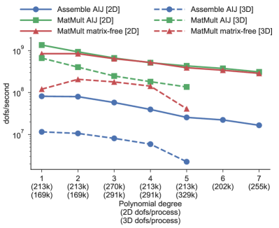
(a) Degrees of freedom per second processed for matrix assembly and matrix-vector products. The performance of matrix-free operator action and assembly at degree 5 in 3D becomes noticeably worse because the data for tabulated basis functions spills from the fastest cache.

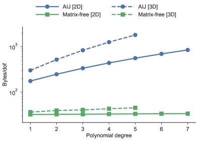
(b) Bytes of memory per degree of freedom. For the matrix-free case, memory usage is not quite constant, since Firedrake stores the ghosted representation, and so a surface-to-volume term appears in the memory per dof (more noticeable in three dimensions).

Figure 1: Performance of matrix-vector products for a Poisson operator discretised on simplices in two and three dimensions (48 MPI processes).

The same story appears for more complex problems, and we show one example, the operator for Rayleigh-Bénard convection discretised using $P_{k+1}$-$P_{k}$-$P_{k}$ elements, in Figure 2. In two dimensions, the matrix-free action is faster than assembled operator application, and in three dimensions the cost is less than a factor 1.5 greater (even at lowest order). Given the high cost of matrix assembly, any iterative method that requires fewer than 10 matrix-vector products will be better off matrix-free, even before memory savings are considered.

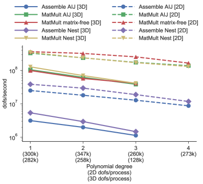
(a) Degrees of freedom per second processed for matrix assembly and matrix-vector products.

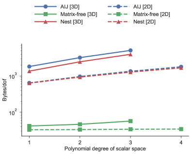
(b) Bytes of memory per degree of freedom.

Figure 2: Performance of matrix-vector products for the Rayleigh-Bénard equation discretised on simplices in two and three dimensions (48 MPI processes).

To determine if these timings are good in absolute terms, we use a roofline model [43]. The arithmetic intensity for assembled matrix-vector products is calculated following [20]. For matrix assembly and matrix-free operator application, we count effective flops in the element kernel by traversing the intermediate representation of the generated code, the required data movement assumes a perfect cache model for any fields (each degree of freedom is only loaded for main memory once), and includes the cost of moving the indirection maps. The spec sheet memory bandwidth per node is $119.4\operatorname{GB/s}$, and we measure a STREAM triad bandwidth of $74.1\operatorname{GB/s}$ per node; the guaranteed not to exceed floating point performance is $518.4\operatorname{Gflop/s}$ per node (one AVX multiplication and one AVX addition issued per cycle per core). As evidenced in Fig. 3, there is almost no extra performance available for the application of assembled operators: the matrix-vector product achieves close to the machine peak in all cases. In contrast, the matrix-free actions, with significantly higher arithmetic intensity, are quite a distance from machine peak: this suggests a direction for future optimisation efforts in Firedrake.

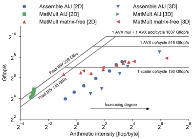
(a) Performance of assembly and matrix-vector products for the Poisson operator. The assembled matrix achieves performance close to machine peak, while matrix-free products (and matrix assembly) are a way away.

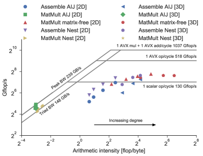
(b) Performance of assembly and matrix-vector products for the Rayleigh-Bénard operator. The nest matrix has higher arithmetic intensity than the aij matrix due to using a blocked CSR format for the diagonal velocity block. As with the Poisson operator, assembled matrices achieve almost machine peak, whereas the matrix-free operator has room for improvement.

Figure 3: Roofline plots for the experiments of Figure 1 and Figure 2.

5.2 Runtime solver composition

5.2.1 Poisson

We now consider solving the Poisson problem Eq. 2 in three dimensions. We choose as domain a regularly meshed unit cube, $\Omega=[0,1]^{d}$, and apply homogenous Dirichlet conditions on $\partial\Omega$, along with a constant forcing term. For low degree discretisations, “black-box” algebraic multigrid methods are robust and provide high performance. Their performance, however, degrades with increasing approximation degree. Here we show how we can plug in the additive Schwarz approach described in Section 3.2 to provide a preconditioner with mesh and degree independent iteration counts, although we do not achieve time to solution independent of these parameters. This increase in time to solution with increasing problem size is due to a non-scalable coarse grid solve: we use algebraic multigrid V cycles.

The main cost of this preconditioner is the application of the (dense) patch inverses, the cost of our implementation is therefore quite high. We also comment that if patch operators are not stored between iterations, the overall memory footprint of the method is quite small. Developing fast algorithms to build and invert these patch operators is the subject of ongoing work.

In Table 1 we compare the algorithmic and runtime performance of hypre’s boomerAMG algebraic multigrid solver applied directly to a $P_{4}$ discretisation with the additive Schwarz approach. The only changes to the application file were in the specification of the runtime solver options. The provided solver options are shown in Section B.1 for the hypre preconditioner and Section B.2 for the Schwarz approach.

Table 1: Krylov iterations, and time to solution for $P_{4}$ Poisson problem using hypre and the Schwarz preconditioner described in Section 3.2 as the problem is weakly scaled. The required number of Krylov iterations grows slowly for the hypre preconditioner, but is constant for Schwarz. However, the overall time to solution is still lower with hypre.

DoFs ($\times 10^{6}$)	MPI processes	Krylov its		Time to solution (s)
		hypre	schwarz	hypre	schwarz
2.571	24	19	19	5.62	9.48
5.545	48	20	19	6.45	10.6
10.22	96	20	19	6.17	10.3
20.35	192	21	18	6.53	10.7
43.99	384	22	19	7.53	11.9
81.18	768	22	19	7.52	11.7
161.9	1536	23	19	8.98	13
350.4	3072	24	19	8.56	14
647.2	6144	26	19	9.32	13.9
1291	12288	28	19	10.2	17.3
2797	24576	29	19	13	22.5

5.2.2 FieldSplit examples

Merely being able to solve the Poisson equation is a relatively uninteresting proposition. The power in our (and PETSc’s) approach is the ease of composition, at runtime, of scalable building blocks to provide preconditioners for complex problems. To demonstrate this, we consider solving the Rayleigh-Bénard equations for stationary convection (7).

A block preconditioner for this problem was developed in [22], but its performance was only studied in two-dimensional systems, and the implementation of the preconditioner was tightly coupled with the problem. The components of this preconditioner are: an inexact inverse of the Navier-Stokes equations, for which the block preconditioners discussed in [18] provide mesh-independent iteration counts; an inexact inverse of the scalar (temperature) convection diffusion operator. For the Navier-Stokes block we approximate the Schur complement with the pressure-convection-diffusion approach (which requires information about the discretisation inside the preconditioner). The building blocks are an approximate inverse for the velocity convection-diffusion operator, and approximate inverses for pressure mass and stiffness matrices. For moderate velocities, the velocity convection-diffusion operator can be treated with algebraic multigrid. Similarly, the pressure mass matrix can be inverted well with only a few iterations of a splitting-based method (e.g. point Jacobi), while multigrid is again good for the stiffness matrix. Finally, the temperature convection-diffusion operator can again be treated with algebraic multigrid.

Using the notation of Eq. 18 and Eq. 22, we need approximate inverses $\widetilde{N}^{-1}$ and $\widetilde{K}^{-1}$. Where $\widetilde{N}^{-1}$ itself needs approximate inverses $\widetilde{F}^{-1}$, $K_{p}^{-1}$, and $M_{p}^{-1}$. We can make different choices for all of these inverses, the matrix format (including matrix-free) for the operators, and convergence tolerance for all approximate inverses. These options (and others) can all be configured at runtime, while maintaining a single code base for the specification of the underlying PDE model, merely by modifying solver options.

Explicitly assembling the Jacobian and inverting with a direct solver requires a relatively short options list: Section B.3. Conversely, to implement the preconditioner of Eq. 22, with algebraic multigrid for all approximate inverses (except the pressure mass matrix), and the operator applied matrix-free, we need significantly more options. These are shown in full in Section B.4.

5.2.3 Algorithmic and parallel scalability

Firedrake and PETSc are designed such that the user of the library need not worry in detail about distributed memory parallelisation, provided they respect the collective semantics of operations. Since our implementation of solvers and preconditioners operates at the level of public APIs, we only need to be careful that we use the correct communicators when constructing auxiliary objects. Parallelisation therefore comes “for free”. In this section, we show that our approach scales to large problem sizes, with scalability limited only by the performance of the building block components of the solver.

We consider the algorithmic performance of the Rayleigh-Bénard problem Eq. 7 in a regularly meshed unit cube, $\Omega=[0,1]^{3}$. We choose as boundary conditions:

(26a) $$u =0\quad\text{on $\partial\Omega$}$$

(26b) $$\nabla p\cdot n =0\quad\text{on $\partial\Omega$}$$

(26c) $$T =1\quad\text{on the plane $x=0$}$$

(26d) $$T =0\quad\text{on the plane $x=1$}$$

(26e) $$\nabla T\cdot n =0\quad\text{otherwise}$$

and take $\text{Ra}=200$ and $\text{Pr}=6.18$. The constant pressure nullspace is projected out in the linear solver. The solution to this problem is shown in Fig. 4.

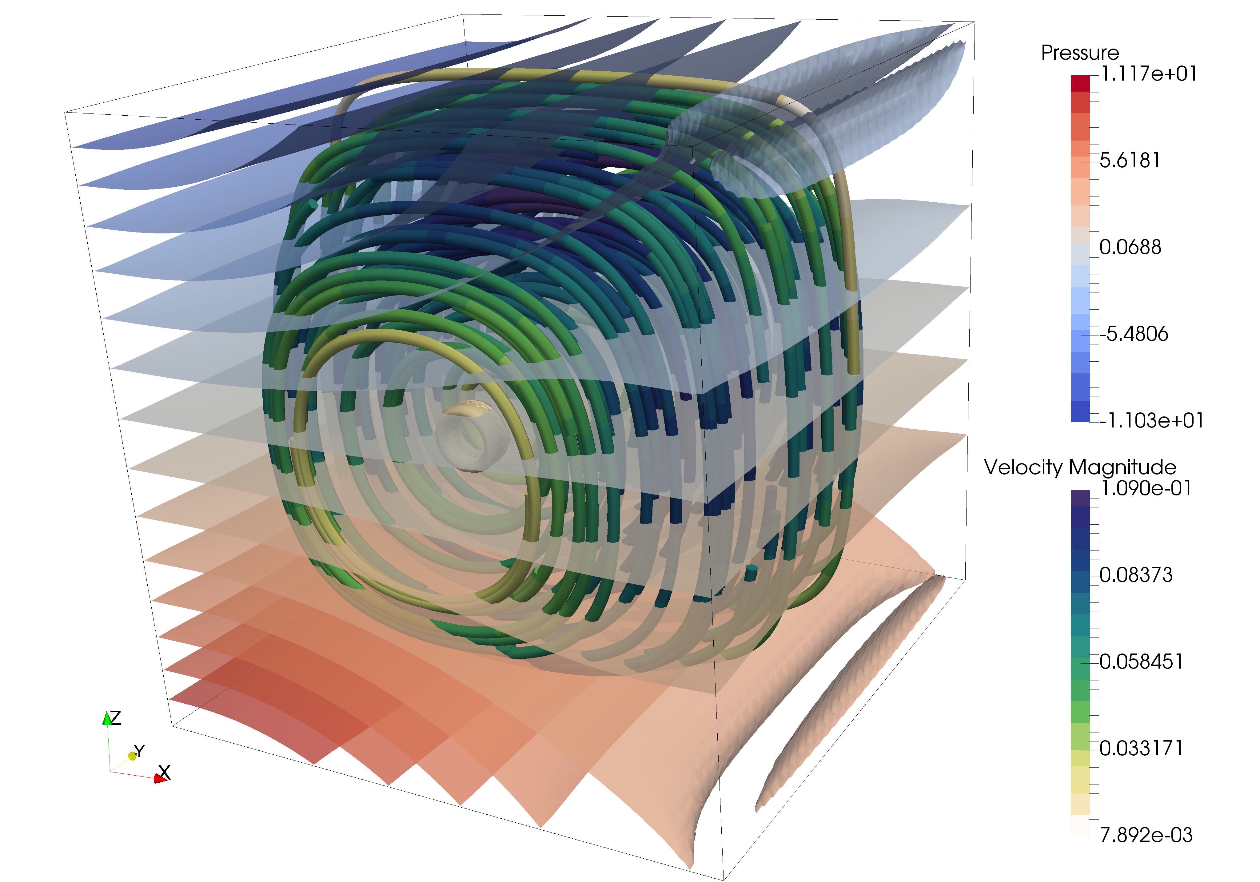
Figure 4: Solution to the Rayleigh-Bénard problem of Eq. 7 with boundary conditions as specified in Eq. 26, and $g$ pointing up. Shown are streamlines of the velocity field coloured by the magnitude of the velocity, and isosurfaces of the pressure.

We perform a weak scaling experiment (increasing both the number of degrees of freedom, and computational resource) to study any mesh dependence in our solver. For the full set of solver options see Section B.4. Newton iterations reduce the residual by $10^{8}$ in three iterations, with only a weak increase in the number of Krylov iterations, as seen in Table 2.

Table 2: Newton iteration counts, total Krylov iterations, and time to solution for Rayleigh-Bénard convection as the problem is weakly scaled. The required number of linear iterations grows slowly as the mesh is refined, however the time to solution grows much faster.

DoFs ($\times 10^{6}$)	MPI processes	Newton its	Krylov its	Time to solution (s)
0.7405	24	3	16	31.7
1.488	48	3	16	36.3
2.973	96	3	17	43.9
5.769	192	3	17	47.3
11.66	384	3	17	56
23.39	768	3	17	64.9
45.54	1536	3	18	85.2
92.28	3072	3	18	120
185.6	6144	3	19	167

The scalability does not look as good as these results would suggest, with only 20% parallel efficiency for this weakly scaled problem on 6144 cores. Looking at the inner solves indicates the problem, although the outer Krylov solve performs well, our approximate inner preconditioners are not fully mesh independent. Table 3 shows the total number of iterations for both the Navier-Stokes solve and the temperature solve as part of the application of the outer preconditioner.

Table 3: Total iterations for Navier-Stokes and temperature solves (with average iterations per outer linear solve in brackets) for the nonlinear solution of the Rayleigh-Bénard problem. We see weak mesh dependence in the per-solve iteration counts. When multiplied up by the slight mesh dependence in the outer solve, this results in a noticeable inefficiency.

DoFs ($\times 10^{6}$)	Navier-Stokes iterations	Temperature iterations
0.7405	329 (20.6)	107 (6.7)
1.488	338 (21.1)	110 (6.9)
2.973	365 (21.5)	132 (7.8)
5.769	358 (21.1)	133 (7.8)
11.66	373 (21.9)	137 (8.1)
23.39	378 (22.2)	139 (8.2)
45.54	403 (22.4)	151 (8.4)
92.28	420 (23.3)	154 (8.6)
185.6	463 (24.4)	174 (9.2)

In addition to iteration counts increasing, the time to compute a single iteration also increases. This is observable more clearly in the previous results for the Poisson operator (Table 1). This is due to sub-optimal scalability of the algebraic multigrid that is used for all the building blocks in these solves. Our results for the Poisson equation using hypre’s boomerAMG appear similar to previously reported results on weak scalability from the hypre team [3], and so we do not expect to gain much improvement here without changing the solver. This can, however, be done without modification to the existing solver: as soon as a better option is available, we can just drop it in.

6 Conclusions and future outlook

We have presented our approach to extending Firedrake and the existing solver interface to support matrix-free operators and the necessary preconditioning infrastructure. Our approach is extensible and composable with existing algebraic solvers supported through PETSc. In particular, it removes much of the friction in developing block preconditioners requiring auxiliary operators. The performance of such preconditioners for complex problems still relies on having good approximate inverses for the blocks, but our composable approach can seamlessly take advantage of any such advances.

Appendix A Code availability

For reproducibility, we cite archives of the exact software versions that were used to produce the results in this paper. The experimentation and job submission framework (along with the plotting scripts and raw results) is available as [46]. The Additive Schwarz preconditioner from Section 3.2 is [53]. For all components of the Firedrake project, we used recent versions: COFFEE [45], FIAT [47], FInAT [48], Firedrake [49], PETSc [50], petsc4py [51], PyOP2 [52], TSFC [54], and UFL [55].

Appendix B Full solver parameters

B.1 Poisson: hypre

We use hypre’s boomerAMG algebraic multigrid implementation, and select more aggressive coarsening strategies to obtain a lower-complexity coarse grid operator than the default.

⬇

-ksp_type cg -ksp_rtol 1e-8 -mat_type aij

-pc_type hypre -pc_hypre_type boomeramg

-pc_hypre_boomeramg_P_max 4

-pc_hypre_boomeramg_no_CF

-pc_hypre_boomeramg_agg_nl 1

-pc_hypre_boomeramg_agg_num_paths 2

-pc_hypre_boomeramg_coarsen_type HMIS

-pc_hypre_boomeramg_interp_type ext+i

B.2 Poisson: schwarz

We use exact inverses for the patch problems, and PETSc’s GAMG algebraic multigrid for the $P_{1}$ inverse. The telescoping preconditioner [34] for the low-order $P_{1}$ operator is used to reduce the number of active MPI processes, since it has many fewer degrees of freedom than the $P_{4}$ operator.

⬇

-ksp_type cg -ksp_rtol 1e-8 -mat_type matfree

-pc_type python -pc_python_type ssc.SSC

-ssc_pc_composite_type additive

-ssc_sub_0_pc_patch_save_operators True

-ssc_sub_0_pc_patch_sub_mat_type seqaij

-ssc_sub_0_sub_ksp_type preonly

-ssc_sub_0_sub_pc_type lu

-ssc_sub_1_lo_pc_type telescope

-ssc_sub_1_lo_pc_telescope_reduction_factor 6

-ssc_sub_1_lo_telescope_ksp_max_it 4

-ssc_sub_1_lo_telescope_ksp_type richardson

-ssc_sub_1_lo_telescope_pc_type gamg

B.3 Rayleigh-Bénard: direct

To invert the full linearised Jacobian with a direct solver (here we use MUMPS [2]), we use the options:

⬇

-mat_type aij

-ksp_type preonly

-pc_type lu

-pc_factor_mat_solver_package mumps

B.4 Rayleigh-Bénard: iterative

To configure the nonlinear iteration, and then also split the Navier-Stokes block from the temperature block, we use:

⬇

-snes_type newtonls -snes_rtol 1e-8 -snes_linesearch_type basic

-ksp_type fgmres -ksp_gmres_modifiedgramschmidt

-mat_type matfree

-pc_type fieldsplit

-pc_fieldsplit_type multiplicative

-pc_fieldsplit_0_fields 0,1

-pc_fieldsplit_1_fields 2

now we configure the temperature solve to use GMRES and algebraic multigrd.

⬇

-prefix_push fieldsplit_1_

-ksp_type gmres

-ksp_rtol 1e-4,

-pc_type python

-pc_python_type firedrake.AssembledPC

-assembled_mat_type aij

-assembled_pc_type telescope

-assembled_pc_telescope_reduction_factor 6

-assembled_telescope_pc_type hypre

-assembled_telescope_pc_hypre_boomeramg_P_max 4

-assembled_telescope_pc_hypre_boomeramg_agg_nl 1

-assembled_telescope_pc_hypre_boomeramg_agg_num_paths 2

-assembled_telescope_pc_hypre_boomeramg_coarsen_type HMIS

-assembled_telescope_pc_hypre_boomeramg_interp_type ext+i

-assembled_telescope_pc_hypre_boomeramg_no_CF True

-prefix_pop

Finally we configure the Navier-Stokes solve to use GMRES with a lower Schur complement factorisation as a preconditioner, and the pressure-convection-diffusion approximation for the schur complement.

⬇

-prefix_push fieldsplit_0_

-ksp_type gmres

-ksp_gmres_modifiedgramschmidt

-ksp_rtol 1e-2

-pc_type fieldsplit

-pc_fieldsplit_type schur

-pc_fieldsplit_schur_fact_type lower

-prefix_push fieldsplit_0_

-ksp_type preonly

-pc_type python

-pc_python_type firedrake.AssembledPC

-assembled_mat_type aij

-assembled_pc_type hypre

-assembled_pc_hypre_boomeramg_P_max 4

-assembled_pc_hypre_boomeramg_agg_nl 1

-assembled_pc_hypre_boomeramg_agg_num_paths 2

-assembled_pc_hypre_boomeramg_coarsen_type HMIS

-assembled_pc_hypre_boomeramg_interp_type ext+i

-assembled_pc_hypre_boomeramg_no_CF

-prefix_pop

-prefix_push fieldsplit_1_

-ksp_type preonly

-pc_type python

-pc_python_type firedrake.PCDPC

-pcd_Fp_mat_type matfree

-pcd_Kp_ksp_type preonly

-pcd_Kp_mat_type aij

-pcd_Kp_pc_type telescope

-pcd_Kp_pc_telescope_reduction_factor 6

-pcd_Kp_telescope_pc_type ksp

-pcd_Kp_telescope_ksp_ksp_max_it 3

-pcd_Kp_telescope_ksp_ksp_type richardson

-pcd_Kp_telescope_ksp_pc_type hypre

-pcd_Kp_telescope_ksp_pc_hypre_boomeramg_P_max 4

-pcd_Kp_telescope_ksp_pc_hypre_boomeramg_agg_nl 1

-pcd_Kp_telescope_ksp_pc_hypre_boomeramg_agg_num_paths 2

-pcd_Kp_telescope_ksp_pc_hypre_boomeramg_coarsen_type HMIS

-pcd_Kp_telescope_ksp_pc_hypre_boomeramg_interp_type ext+i

-pcd_Kp_telescope_ksp_pc_hypre_boomeramg_no_CF

-pcd_Mp_mat_type aij

-pcd_Mp_ksp_type richardson

-pcd_Mp_pc_type sor

-pcd_Mp_ksp_max_it 2

-prefix_pop

-prefix_pop

References

- [1] M. S. Alnæs, A. Logg, K. B. Ølgaard, M. E. Rognes, and G. N. Wells, Unified Form Language: a domain-specific language for weak formulations of partial differential equations, ACM Transactions on Mathematical Software, 40 (2014), https://doi.org/10.1145/2566630, https://arxiv.org/abs/1211.4047.
- [2] P. R. Amestoy, I. S. Duff, and J.-Y. L’Excellent, Multifrontal parallel distributed symmetric and unsymmetric solvers, Computer methods in applied mechanics and engineering, 184 (2000), pp. 501–520, https://doi.org/10.1016/S0045-7825(99)00242-X.
- [3] A. H. Baker, R. D. Falgout, T. Gamblin, T. V. Kolev, M. Schulz, and U. M. Yang, Scaling algebraic multigrid solvers: on the road to exascale, in Competence in High Performance Computing 2010: Proceedings of an International Conference on Competence in High Performance Computing, June 2010, Schloss Schwetzingen, Germany, C. Bischof, H.-G. Hegering, W. E. Nagel, and G. Wittum, eds., Berlin, Heidelberg, 2012, Springer Berlin Heidelberg, pp. 215–226, https://doi.org/10.1007/978-3-642-24025-6_18.
- [4] S. Balay, S. Abhyankar, M. F. Adams, J. Brown, P. Brune, K. Buschelman, L. Dalcin, V. Eijkhout, W. D. Gropp, D. Kaushik, M. G. Knepley, L. C. McInnes, K. Rupp, B. F. Smith, S. Zampini, H. Zhang, and H. Zhang, PETSc Users Manual, Tech. Report ANL-95/11 - Revision 3.7, Argonne National Laboratory, 2016.
- [5] S. Balay, W. D. Gropp, L. C. McInnes, and B. F. Smith, Efficient management of parallelism in object oriented numerical software libraries, in Modern Software Tools in Scientific Computing, E. Arge, A. M. Bruaset, and H. P. Langtangen, eds., Birkhäuser Press, 1997, pp. 163–202, https://doi.org/10.1007/978-1-4612-1986-6_8.
- [6] M. Benzi, G. Golub, and J. Liesen, Numerical solution of saddle point problems, Acta Numerica, 14 (2005), pp. 1–137, https://doi.org/10.1017/S0962492904000212.
- [7] A. Brandt, Multi-level adaptive solutions to boundary-value problems, Mathematics of Computation, 31 (1977), pp. 333–390, https://doi.org/10.1090/S0025-5718-1977-0431719-X.
- [8] A. Brandt and O. Livne, Multigrid Techniques, Society for Industrial and Applied Mathematics, 2011, https://doi.org/10.1137/1.9781611970753.
- [9] S. C. Brenner and L. R. Scott, The mathematical theory of finite element methods, vol. 15 of Texts in Applied Mathematics, Springer, New York, third edition ed., 2008.
- [10] J. Brown, M. G. Knepley, D. A. May, L. C. McInnes, and B. F. Smith, Composable linear solvers for multiphysics, in Proceedings of the 2012 11th International Symposium on Parallel and Distributed Computing, ISPDC ’12, Washington, DC, USA, 2012, IEEE Computer Society, pp. 55–62, https://doi.org/10.1109/ISPDC.2012.16.
- [11] G. F. Carey and T. J. Oden, Finite Elements: Fluid Mechanics Vol., VI, Prentice-Hall, Inc., 1986.
- [12] E. C. Cyr, J. N. Shadid, and R. S. Tuminaro, Teko: A block preconditioning capability with concrete example applications in Navier-Stokes and MHD, SIAM Journal on Scientific Computing, 38 (2016), pp. S307–S331, https://doi.org/10.1137/15M1017946.
- [13] L. D. Dalcin, R. R. Paz, P. A. Kler, and A. Cosimo, Parallel distributed computing using Python, Advances in Water Resources, 34 (2011), pp. 1124–1139, https://doi.org/10.1016/j.advwatres.2011.04.013. New Computational Methods and Software Tools.
- [14] T. A. Davis, Algorithm 832: UMFPACK V4.3-an unsymmetric-pattern multifrontal method, ACM Transactions on Mathematical Software, 30 (2004), pp. 196–199, https://doi.org/10.1145/992200.992206.
- [15] H. Elman, V. E. Howle, J. Shadid, R. Shuttleworth, and R. Tuminaro, Block preconditioners based on approximate commutators, SIAM Journal on Scientific Computing, 27 (2006), pp. 1651–1668, https://doi.org/10.1137/040608817.
- [16] H. Elman, V. E. Howle, J. Shadid, R. Shuttleworth, and R. Tuminaro, A taxonomy and comparison of parallel block multi-level preconditioners for the incompressible Navier–Stokes equations, Journal of Computational Physics, 227 (2008), pp. 1790–1808, https://doi.org/10.1016/j.jcp.2007.09.026.
- [17] H. Elman and D. Silvester, Fast nonsymmetric iterations and preconditioning for Navier-Stokes equations, SIAM Journal on Scientific Computing, 17 (1996), pp. 33–46, https://doi.org/10.1137/0917004.
- [18] H. Elman, D. Silvester, and A. Wathen, Finite elements and fast iterative solvers, Oxford University Press, second edition ed., 2014.
- [19] P. E. Farrell and J. W. Pearson, A preconditioner for the Ohta-Kawasaki equation, 2016, https://arxiv.org/abs/1603.04570.
- [20] W. D. Gropp, D. K. Kaushik, D. E. Keyes, and B. F. Smith, Towards realistic performance bounds for implicit CFD codes, in Parallel CFD 1999, D. Keyes, A. Ecer, J. Periaux, and N. Satofuka, eds., North-Holland, 2000, pp. 241–248, https://doi.org/10.1016/B978-044482851-4.50030-X.
- [21] M. A. Heroux, R. A. Bartlett, V. E. Howle, R. J. Hoekstra, J. J. Hu, T. G. Kolda, R. B. Lehoucq, K. R. Long, R. P. Pawlowski, E. T. Phipps, A. G. Salinger, H. K. Thornquist, R. S. Tuminaro, J. M. Willenbring, A. Williams, and K. S. Stanley, An overview of the Trilinos project, ACM Transactions on Mathematical Software, 31 (2005), pp. 397–423, https://doi.org/10.1145/1089014.1089021.
- [22] V. E. Howle and R. C. Kirby, Block preconditioners for finite element discretization of incompressible flow with thermal convection, Numerical Linear Algebra with Applications, 19 (2012), pp. 427–440, https://doi.org/10.1002/nla.1814.
- [23] V. E. Howle, R. C. Kirby, K. Long, B. Brennan, and K. Kennedy, Playa: high-performance programmable linear algebra, Scientific Programming, 20 (2012), pp. 257–273, https://doi.org/10.1155/2012/606215.
- [24] B. Jessic, D. Kay, M. Stoll, and A. J. Wathen, Fast solvers for Cahn-Hilliard inpainting, SIAM Journal on Imaging Sciences, 7 (2014), pp. 67–97, https://doi.org/10.1137/130921842.
- [25] D. Kay, D. Loghin, and A. Wathen, A preconditioner for the steady-state Navier-Stokes equations, SIAM Journal on Scientific Computing, 24 (2002), pp. 237–256, https://doi.org/10.1137/S106482759935808X.
- [26] R. C. Kirby, Algorithm 839: FIAT, a new paradigm for computing finite element basis functions, ACM Transactions on Mathematical Software, 30 (2004), pp. 502–516, https://doi.org/10.1145/1039813.1039820.
- [27] M. G. Knepley and D. A. Karpeev, Mesh Algorithms for PDE with Sieve I: Mesh Distribution, Scientific Programming, 17 (2009), pp. 215–230, https://doi.org/10.1155/2009/948613.
- [28] A. Logg, K.-A. Mardal, and G. N. Wells, eds., Automated solution of differential equations by the finite element method: the FEniCS book, vol. 84, Springer, 2012, https://doi.org/10.1007/978-3-642-23099-8.
- [29] K. Long, R. C. Kirby, and B. van Bloemen Waanders, Unified embedded parallel finite element computations via software-based Fréchet differentiation, SIAM Journal on Scientific Computing, 32 (2010), pp. 3323–3351, https://doi.org/10.1137/09076920X.
- [30] K. R. Long, Sundance rapid prototyping tool for parallel PDE optimization, in Large-Scale PDE-Constrained Optimization, L. T. Biegler, M. Heinkenschloss, O. Ghattas, and B. van Bloemen Waanders, eds., Springer Berlin Heidelberg, Berlin, Heidelberg, 2003, pp. 331–341, https://doi.org/10.1007/978-3-642-55508-4_20.
- [31] K.-A. Mardal and J. B. Haga, Automated solution of differential equations by the finite element method: the FEniCS book, in Logg et al. [28], ch. Block preconditioning of systems of PDEs, https://doi.org/10.1007/978-3-642-23099-8.
- [32] K.-A. Mardal and R. Winther, Preconditioning discretizations of systems of partial differential equations, Numerical Linear Algebra with Applications, 18 (2011), pp. 1–40, https://doi.org/10.1002/nla.716.
- [33] D. A. May, J. Brown, and L. Le Pourhiet, pTatin3D: High-performance methods for long-term lithospheric dynamics, in Proceedings of the International Conference for High Performance Computing, Networking, Storage and Analysis, SC ’14, Piscataway, NJ, USA, 2014, IEEE Press, pp. 274–284, https://doi.org/10.1109/SC.2014.28.
- [34] D. A. May, P. Sanan, K. Rupp, M. G. Knepley, and B. F. Smith, Extreme-scale multigrid components within PETSc, in Proceedings of the Platform for Advanced Scientific Computing Conference, PASC ’16, New York, NY, USA, 2016, ACM, pp. 5:1–5:12, https://doi.org/10.1145/2929908.2929913, https://arxiv.org/abs/1604.07163.
- [35] J. D. McCalpin, Memory Bandwidth and Machine Balance in Current High Performance Computers, IEEE Computer Society Technical Committee on Computer Architecture Newsletter, (1995), pp. 19–25.
- [36] M. F. Murphy, G. H. Golub, and A. J. Wathen, A note on preconditioning for indefinite linear systems, SIAM Journal on Scientific Computing, 21 (2000), pp. 1969–1972, https://doi.org/10.1137/S1064827599355153.
- [37] L. F. Pavarino, Additive Schwarz methods for the -version finite element method, Numerische Mathematik, 66 (1993), pp. 493–515, https://doi.org/10.1007/BF01385709.
- [38] L. F. Pavarino, Schwarz methods with local refinement for the -version finite element method, Numerische Mathematik, 69 (1994), pp. 185–211, https://doi.org/10.1007/s002110050087.
- [39] L. F. Pavarino and T. Warburton, Overlapping Schwarz methods for unstructured spectral elements, Journal of Computational Physics, 160 (2000), pp. 298–317, https://doi.org/10.1006/jcph.2000.6463.
- [40] F. Rathgeber, D. A. Ham, L. Mitchell, M. Lange, F. Luporini, A. T. T. McRae, G.-T. Bercea, G. R. Markall, and P. H. J. Kelly, Firedrake: automating the finite element method by composing abstractions, ACM Transactions on Mathematical Software, 43 (2016), pp. 24:1–24:27, https://doi.org/10.1145/2998441, https://arxiv.org/abs/1501.01809.
- [41] Y. Saad, Iterative Methods for Sparse Linear Systems, Society for Industrial and Applied Mathematics, second edition ed., 2003, https://doi.org/10.1137/1.9780898718003.
- [42] J. Schöberl, J. M. Melenk, C. Pechstein, and S. Zaglmayr, Additive Schwarz preconditioning for -version triangular and tetrahedral finite elements, IMA Journal of Numerical Analysis, 28 (2008), pp. 1–24, https://doi.org/10.1093/imanum/drl046.
- [43] S. Williams, A. Waterman, and D. Patterson, Roofline: An insightful visual performance model for multicore architectures, Communications of the ACM, 52 (2009), pp. 65–76, https://doi.org/10.1145/1498765.1498785.
- [44] J. Xu, Iterative methods by space decomposition and subspace correction, SIAM review, 34 (1992), pp. 581–613, https://doi.org/10.1137/1034116.
- [45] Zenodo/COFFEE, COFFEE: A Compiler for Fast Expression Evaluation, Dec. 2016, https://doi.org/10.5281/zenodo.208989.
- [46] Zenodo/composable-solvers, composable-solvers: experimentation framework for composable block preconditioners, Oct. 2017, https://doi.org/10.5281/zenodo.1014582.
- [47] Zenodo/FIAT, FIAT: The Finite Element Automated Tabulator, June 2017, https://doi.org/10.5281/zenodo.802269.
- [48] Zenodo/FInAT, FInAT: a smarter library of finite elements, June 2017, https://doi.org/10.5281/zenodo.802275.
- [49] Zenodo/Firedrake, Firedrake: an automated finite element system, June 2017, https://doi.org/10.5281/zenodo.802271.
- [50] Zenodo/PETSc, PETSc: Portable, Extensible Toolkit for Scientific Computation, June 2017, https://doi.org/10.5281/zenodo.802273.
- [51] Zenodo/petsc4py, petsc4py: The Python interface to PETSc, June 2017, https://doi.org/10.5281/zenodo.802274.
- [52] Zenodo/PyOP2, PyOP2: Framework for performance-portable parallel computations on unstructured meshes, June 2017, https://doi.org/10.5281/zenodo.802272.
- [53] Zenodo/SSC, SSC: subspace corrections in Firedrake & PETSc, June 2017, https://doi.org/10.5281/zenodo.802279.
- [54] Zenodo/TSFC, TSFC: The Two Stage Form Compiler, June 2017, https://doi.org/10.5281/zenodo.802268.
- [55] Zenodo/UFL, UFL: The Unified Form Language, June 2017, https://doi.org/10.5281/zenodo.802270.