Abstract

We construct the holographic renormalization group (RG) flow of thermo-electric conductivities when the translational symmetry is broken. The RG flow is probed by the intrinsic observers hovering on the sliding radial membranes. We obtain the RG flow by solving a matrix-form Riccati equation. The RG flow provides a high-efficient numerical method to calculate the thermo-electric conductivities of strongly coupled systems with momentum dissipation. As an illustration, we recover the AC thermo-electric conductivities in the Einstein-Maxwell-axion model. Moreover, in several homogeneous and isotropic holographic models which dissipate the momentum and have the finite density, it is found that the RG flow of a particular combination of DC thermo-electric conductivities does not run. As a result, the DC thermal conductivity on the boundary field theory can be derived analytically, without using the conserved thermal current.

1 Introduction

“GR=RG” [1]. In the holographic theory, this short “equation” highlights that the renormalization group (RG), an iterative coarse-graining scheme to extract the relevant physics [2, 3, 4], is essential in generating the bulk gravity dual from the boundary field theory. Although the precise process of coarse graining is not clear, it is evident that the anti-de Sitter/conformal field theory (AdS/CFT) correspondence provides the geometrisation of RG flow, in which the radial direction in the bulk can be identified with certain energy scale [5, 6, 7, 8, 9, 10, 11, 12, 13, 14, 15, 16, 17]. As an important implication of this picture, one can expect that some low-energy universality of strongly coupled systems is captured by the near-horizon degrees of freedom alone.

On the other hand, as Pauli said, “Solid state physics is dirty”. The disorder is one of the fundamental themes in condensed matter theories (CMT). It is an important progress that the AdS/CMT duality can dissipate the momentum and thereby get close to the real materials. The simplest way to break the translational symmetry in the holographic theories is to introduce the linear axion fields [18].

Recently, some of us studied the holographic RG flow for the strongly coupled systems with finite density and disorder [19, 20, 21], where the charge and energy transport are coupled and the transport coefficients are finite. The partial motivation of the work came from Ref. [22], where the authors have not obtained the explicit flow when facing with the coupled transport. By introducing a square matrix of coupled sources, we illustrated that the coupled second-order equations of linear perturbations can be reduced to a first-order matrix Riccati equation, which can have the direct physical meaning of the RG flow equation of two-point correlation functions [21]. In addition, the boundary condition of the matrix Riccati equation can be simply determined by the regularity of correlation functions on the horizon. As a result, the holographic RG flow provides a new method for calculating the coupled transport in holographic systems, particularly with translational symmetry breaking. Compared with the traditional method that solves the coupled second-order perturbation equations directly, the new method can greatly simplify the numerical calculation, particularly for the AC transport or spatially inhomogeneous systems. This is mainly because it only needs a simple Runge-Kutta marching instead of the inconvenient shooting method or the resource-consuming pseudo-spectral method.

In [19, 20, 21], however, the holographic RG flow was mainly used to study the DC transport on the boundary. In this paper, the first aim is to translate the matrix Riccati equation to the RG flow of AC thermo-electric conductivities, from which one can read the AC thermo-electric conductivities on the boundary. As an illustration, we will calculate these conductivities in the Einstein-Maxwell-axion (EMA) model. The results are in agreement with the previous work [23] that solves the coupled second-order equations directly.

The second aim is to explore whether the holographic RG flow could imply some interesting physics about the thermo-electric transport in strongly coupled systems. One important lesson learned from the studies on the holographic RG flow is that the universality of the transport in the holographic models may be correlated to the similarity of all horizons and the existence of certain quantities which do not evolve between the horizon and the boundary [24]. Two benchmark examples are the trivial RG flow of the DC electrical conductivity for the systems dual to neutral black holes and the ratio between shear viscosity and entropy density in a wide class of holographic theories. Notably, the trivial RG flow interpolates the classical black hole membrane paradigm [25, 26] and AdS/CFT smoothly. Based on this universality argument, Blake and Tong identified a massless mode in the massive gravity and obtained the analytical expression of the DC electric conductivity [27]. Furthermore, Donos and Gauntlett constructed the electric and thermal currents that are radially conserved. Combined with the choice of sources that are linear in time, they found an analytical relation between the DC thermo-electric conductivities on the boundary and the black hole horizon data [28]. However, unlike the conserved electric current that usually can be read from the Maxwell equation, the construction of the conserved thermal current is considerably more subtle. Noticing this problem, Liu, Lu, and Pope recently suspected that the Noether current with respect to the diffeomorphism symmetry might be a general formula for the radially conserved thermal current [29].

We will show that the RG flow of a particular combination of DC thermo-electric conductivities, namely, the electrical conductivity at zero heat current, does not run in several homogeneous and isotropic holographic models which dissipate the momentum and have the finite density. Since the zero-heat-current (ZHC) conductivity at zero density is reduced to the electrical conductivity, the trivial flow of ZHC conductivity can be naturally viewed as the nontrivial extension of the zero-density electrical conductivity flow [24]. Furthermore, given the analytical expression of electric and thermoelectric conductivities that can be obtained from the conserved electric current, we can derive the thermal conductivity analytically by using the trivial RG flow of ZHC conductivity and the infrared boundary condition of the matrix Riccati equation. The radially conserved thermal current is not required.

The rest of this paper is organized as follows. In Sec. 2, we will develop a general framework for the holographic RG flow of the thermo-electric transport. In Sec. 3, we will take the EMA model as an example which exhibits how the RG flow can be used to calculate the AC thermo-electric conductivities on the boundary. The RG flow of the DC thermo-electric conductivities will be studied in Sec. 4. By the numerical method, one can find that the ZHC conductivity has a trivial flow in various holographic models. This further induces an analytical expression of the DC thermal conductivity, as will be shown in Sec. 5. In the last section, the conclusion will be given. In two appendices, we will present the thermodynamics on the membranes and a semi-analytical proof for the trivial RG flow, respectively.

2 Thermo-electric RG flow: a general framework

One of the well-known approaches to the holographic RG is the (sliding) membrane paradigm proposed in [24]. It is technically convenient to relate the linear response measured by the observers hovering outside the horizon to that of the boundary theory. Such relation is also exhibited in the Wilsonian approach to fluid/gravity duality [30]. The flow equations obtained in [24] can be retrieved as the $\beta$-functions of double-trace couplings by the holographic Wilsonian RG approach which integrates out the ultraviolet geometry [31, 32, 33]. The equivalence between the membrane paradigm and the holographic Wilsonian RG has been further discussed in [34, 22].

Until now, the holographic RG flow of the complete thermo-electric transport has not been studied and we will develop the previous membrane paradigm to fill this gap. Our essential idea is to associate a positioned action with a sliding membrane and reformulate the classical equations of motion (EOM) to the RG flow of transport coefficients which are measured by intrinsic observers.

In linear response, the change in the expectation value of any operator $O_{I}$ is assumed to be linear in the perturbing source $\phi_{I}$

$$\delta\left\langle O_{I}\left(\omega\right)\right\rangle=G_{R}^{IJ}\left(\omega\right)\phi_{I}\left(\omega\right),$$ (1)

where $G_{R}^{IJ}$ is the retarded Green’s function

$$G_{R}^{IJ}(\omega)\equiv-i\int_{0}^{\infty}dte^{i\omega t}\langle\left[O_{I}(t),O_{J}(0)\right]\rangle.$$ (2)

In holography, by recasting the on-shell quadratic action as the form

$$S_{\mathrm{os}}^{(2)}=\frac{1}{2}\int\frac{d\omega}{2\pi}\phi_{I}\left(-\omega\right)G_{IJ}\left(\omega\right)\phi_{J}\left(\omega\right),$$ (3)

the retarded Green’s function can be extracted [35], up to the contact term [36]. In [21], it has been shown that the coupled perturbation equations in the bulk can be reformulated as a matrix-form Riccati equation:

$$\Gamma^{\prime}=M-N\Gamma-\Gamma\tilde{N}-\Gamma O\Gamma.$$ (4)

Here $\Gamma_{IJ}\equiv G_{IJ}/\left(i\omega\right)$ is referred to the canonical response function and the matrices $M$, $N$, $\tilde{N}$ and $O$ are independent of perturbations. They are the functions of radial coordinate $r$ and the prime denotes the radial derivative. In the following, we will translate $G_{IJ}(r)$ and hence $\Gamma_{IJ}(r)$ into the RG flow of thermo-electric conductivities. Note that the process is general for any theories of gravity which will be considered in this paper.

In terms of the standard AdS/CFT correspondence, the $\left(d+1\right)$-dimensional field theory lives on a conformal class of the asymptotic boundary of the $\left(d+2\right)$-dimensional bulk spacetime. The radial coordinate in the bulk can be identified with certain energy scale. As a direct extrapolation, we assume that the field theory at certain energy scale is associated with a fictitious membrane at the radial cutoff $r=r_{c}$, with the line element

$$ds^{2}=\frac{1}{\Lambda(r_{c})^{2}}\gamma_{ab}(r_{c})dx^{a}dx^{b}.$$ (5)

Here $\gamma_{ab}$ is the induced metric, with $a,b\in\left\{0,\cdots,d\right\}$. To be simple, it is assumed to be homogeneous and isotropic. Its spatial component is denoted as $\gamma_{ij}$, with $i,j\in\left\{1,\cdots,d\right\}$. We define $\lambda_{ab}\equiv\gamma_{ab}/\Lambda(r_{c})^{2}$ as the membrane metric, which is determined up to a conformal factor $\Lambda(r_{c})^{2}$ that will be specified later.

Consider that the observers on the membranes are equipped with the proper intrinsic coordinates,

$$\hat{t}=\frac{\sqrt{-\gamma_{00}(r_{c})}}{\Lambda(r_{c})}t,\;\hat{x}^{i}=\frac{\sqrt{\gamma_{ii}(r_{c})}}{\Lambda(r_{c})}x^{i}.$$ (6)

Put differently, the intrinsic observers measure the physical quantities by the orthonormal bases. For the sake of brevity, we will describe the positioned physical quantities as “observed” when they are measured by the intrinsic observers lived on the membranes. To be clear, we hat on all observed quantities. We choose to hat the vector or tensor on the index.

We need to define the positioned on-shell action, which involves three parts

$$S_{\mathrm{os}}=\left.\left(S_{\mathrm{bulk}}+S_{\mathrm{GH}}+S_{\mathrm{ct}}\right)\right|_{\mathrm{on-shell}}.$$ (7)

The first is the bulk action

$$S_{\mathrm{bulk}}=\int_{r_{+}}^{r_{c}}d^{d+2}x\sqrt{-g}\mathcal{L}.$$ (8)

In the AdS/CFT correspondence, the field theory lives on the boundary and the ultraviolet limit (that we suppose to be $r_{c}\rightarrow\infty$) is imposed. Here we consider the bulk region from the horizon $r_{+}$ to certain cutoff surface with $r_{c}>r_{+}$, giving rise to the $r_{c}$-dependence of the action. Second, to implement a well-defined variational principle, the Gibbons-Hawking term on the cutoff surface is necessary. The last is the counterterm, which is required in AdS/CFT to cancel the ultraviolet divergence. To obtain a continuous RG flow, we extend the counterterm to arbitrary slices following Ref. [22].

We proceed to define the electric current and energy-momentum current on the membranes, which are covariant,

$$J^{a}=\frac{1}{\sqrt{-\lambda}}\frac{\delta S_{\mathrm{os}}}{\delta A_{a}},\;T^{ab}=\frac{2}{\sqrt{-\lambda}}\frac{\delta S_{\mathrm{os}}}{\delta\lambda_{ab}},$$ (9)

where $\lambda$ is the determinant of the membrane metric. For our purpose, we set $x=x^{1}$ and focus on the relevant components $\left(J_{x},T_{tx}\right)\,$. They are observed by

$$J_{\hat{x}} = \frac{\Lambda}{\sqrt{\gamma_{11}}}J_{x}=\frac{\sqrt{\gamma_{11}}}{\sqrt{-\gamma_{00}}}\frac{1}{\sqrt{\lambda_{d}}}\frac{\delta S_{\mathrm{os}}}{\delta A_{x}},$$

$$T_{\hat{t}\hat{x}} = \frac{\Lambda}{\sqrt{\gamma_{11}}}\frac{\Lambda}{\sqrt{-\gamma_{00}}}T_{tx}=-\frac{\sqrt{\gamma_{11}}}{\Lambda}\frac{1}{\sqrt{\lambda_{d}}}\frac{\delta S_{\mathrm{os}}}{\delta\lambda_{tx}}.$$ (10)

where $\delta\lambda_{xt}=\delta\lambda_{tx}$ has been used. With these quantities at hand, the observed thermo-electric conductivities can be defined through the generalized Ohm’s law

$$\left(\begin{array}[]{c}J_{\hat{x}}\\ J_{\hat{x}}^{Q}\end{array}\right)=\left(\begin{array}[]{cc}\hat{\sigma}&\hat{T}\hat{\alpha}\\ \hat{T}\hat{\alpha}&\hat{T}\hat{\kappa}\end{array}\right)\left(\begin{array}[]{c}E_{\hat{x}}\\ -\nabla_{{}_{\hat{x}}}\hat{T}/\hat{T}\end{array}\right),$$ (11)

where the Tolman temperature on the membrane is determined by the Hawking temperature and the redshift factor, that is, $\hat{T}\left(r_{c}\right)=T\frac{\Lambda(r_{c})}{\sqrt{-\gamma_{00}(r_{c})}}$. Note that the Tolman temperature is the only observed thermodynamic quantity which is necessary for calculating the observed thermo-electric conductivities. Nevertheless, we will study in Appendix A the complete and self-consistent observed thermodynamics, which should be important in itself.

We will relate the sources $E_{\hat{x}}$ and $\nabla_{{}_{\hat{x}}}\hat{T}$ to the fluctuations $\delta A_{{}_{\hat{x}}}$ and $\delta\lambda_{\hat{t}\hat{x}}$, following Sec. 2.7 in [37]. Consider the spacetime associated with the metric $\lambda_{\hat{a}\hat{b}}$ that is nothing but the Minkowski metric. Rescale the time by $\hat{t}\rightarrow\bar{t}/\hat{T}$ and then the metric has $\lambda_{\bar{t}\bar{t}}=-1/\hat{T}^{2}$. Turn on a small constant thermal gradient $\hat{T}\rightarrow\hat{T}-\hat{x}\nabla_{\hat{x}}\hat{T}$. It implies $\delta\lambda_{\bar{t}\bar{t}}=-2\hat{x}\nabla_{\hat{x}}\hat{T}/\hat{T}^{3}$. The fluctuation can be compensated by the diffeomorphism $\delta\lambda_{\bar{t}\bar{t}}=2\partial_{\bar{t}}\xi_{\bar{t}}$ with the parameter $\xi_{\bar{t}}=i\hat{x}\nabla_{\hat{x}}\hat{T}/\left(\bar{\omega}\hat{T}^{3}\right)$. Here we have endowed all quantities with a time dependence $e^{-i\bar{\omega}\bar{t}}$. Taking $\xi_{\hat{x}}=0$, the diffeomorphisms $\delta\lambda_{\bar{t}\hat{x}}=\partial_{\hat{x}}\xi_{\bar{t}}$ and $\delta A_{\hat{x}}=A_{\bar{t}}\partial_{\hat{x}}\xi^{\bar{t}}$ can induce $\delta\lambda_{\bar{t}\hat{x}}=i\nabla_{\hat{x}}\hat{T}/\left(\bar{\omega}\hat{T}^{3}\right)$ and $\delta A_{\hat{x}}=-iA_{\bar{t}}\nabla_{\hat{x}}\hat{T}/\left(\bar{\omega}\hat{T}\right)$, respectively. Rescaling back to the original time $\hat{t}$, one can obtain the net effect of the thermal gradient $i\hat{\omega}\delta\lambda_{\hat{t}\hat{x}}=-\nabla_{{}_{\hat{x}}}\hat{T}/\hat{T}$ and $i\hat{\omega}\delta A_{\hat{x}}=A_{\hat{t}}\nabla_{\hat{x}}\hat{T}/\hat{T}$. Combined with the relation $E_{\hat{x}}=i\hat{\omega}\delta A_{{}_{\hat{x}}}$ when the electric field is turned on, we can read

$$E_{\hat{x}}+A_{\hat{t}}\nabla_{{}_{\hat{x}}}\hat{T}/\hat{T}=i\hat{\omega}\delta A_{{}_{\hat{x}}},\;\nabla_{{}_{\hat{x}}}\hat{T}/\hat{T}=-i\hat{\omega}\delta\lambda_{\hat{t}\hat{x}}.$$ (12)

Furthermore, the variation of the on-shell action takes the form

$$\delta S_{\mathrm{os}} = \int d^{d+1}x\left(\frac{\delta S_{\mathrm{os}}}{\delta A_{x}}\delta A_{x}+\frac{\delta S_{\mathrm{os}}}{\delta\gamma_{tx}}\delta\gamma_{tx}\right)$$ (13)

$$= \int d^{d+1}x\sqrt{-\lambda}\left(J^{x}\delta A_{x}+T^{tx}\delta\lambda_{tx}\right)$$

$$= \int d^{d+1}\hat{x}\sqrt{-\hat{\lambda}}\left(J^{\hat{x}}\delta A_{{}_{\hat{x}}}+T^{\hat{t}\hat{x}}\delta\lambda_{\hat{t}\hat{x}}\right)$$

$$= \int d^{d+1}\hat{x}\sqrt{-\hat{\lambda}}\left[J^{\hat{x}}\frac{E_{\hat{x}}}{i\hat{\omega}}-\left(T_{\hat{t}}^{\hat{x}}+A_{\hat{t}}J^{\hat{x}}\right)\frac{-\nabla_{{}_{\hat{x}}}\hat{T}}{i\hat{\omega}\hat{T}}\right].$$

In the second line, we have used Eq. (9) and $\delta\lambda_{tx}=\delta\gamma_{tx}/\Lambda(r_{c})^{2}$. The third line denotes a coordinate transformation. In terms of Eq. (12) we obtain the last line, where the heat current can be recognised

$$J_{\hat{x}}^{Q}=-\left(T_{\hat{t}\hat{x}}+A_{\hat{t}}J_{\hat{x}}\right).$$ (14)

Putting Eq. (10) and Eq. (14) into Eq. (11), we can represent $\left(\hat{\sigma},\hat{\alpha},\hat{\kappa}\right)$ by

$$\hat{\sigma} = \frac{1}{i\omega}G_{11}\frac{\gamma_{11}}{\sqrt{\lambda_{d}}\Lambda^{2}},$$

$$\hat{\alpha} = \frac{1}{i\omega}\frac{\left(-G_{12}\gamma_{00}-G_{11}\gamma_{11}A_{t}\right)}{\sqrt{\lambda_{d}}\Lambda^{2}T},$$

$$\hat{\kappa} = \frac{1}{i\omega}\frac{1}{\gamma_{11}\sqrt{\lambda_{d}}\Lambda\sqrt{-\gamma_{00}}T}\left[G_{11}\gamma_{11}^{2}A_{t}^{2}+\left(G_{12}+G_{21}\right)\gamma_{00}\gamma_{11}A_{t}+\left(G_{22}-C_{22}\right)\gamma_{00}^{2}\right].$$ (15)

Here we have defined the correlator $G_{IJ}$ by Eq. (3). The sources $\varphi_{I}=\left(a_{x},h_{tx}\right)$ come from

$$\delta\gamma_{tx}=\gamma_{11}(r)h_{tx}(r)e^{-i\omega t},\;\delta A_{x}=a_{x}(r)e^{-i\omega t}.$$ (16)

It should be noted that the contact term $C_{22}\equiv G_{22}\left(0\right)$ (that appears in all the models of this paper) has been subtracted in Eq. (15), otherwise there is a pole at $\omega=0$ in the imaginary part of $\hat{\kappa}$ [23]. The observed ZHC conductivity is defined by

$$\hat{\sigma}_{\mathrm{0}}\equiv\left.\frac{J_{\hat{x}}}{E_{\hat{x}}}\right|_{J_{\hat{x}}^{Q}=0}=\hat{\sigma}-\frac{\hat{T}\hat{\alpha}^{2}}{\hat{\kappa}}.$$ (17)

From Eq. (15), it can be expressed as

$$\hat{\sigma}_{\mathrm{0}}=\frac{1}{i\omega}\frac{-\gamma_{00}G_{11}}{\sqrt{\lambda_{d}}\Lambda^{2}}\frac{G_{11}\left(G_{12}-G_{21}\right)\gamma_{11}A_{t}-\left[G_{11}\left(G_{22}-C_{22}\right)-G_{12}^{2}\right]\gamma_{00}}{G_{11}A_{t}^{2}\gamma_{11}^{2}+\left(G_{12}+G_{21}\right)\gamma_{00}\gamma_{11}A_{t}+\left(G_{22}-C_{22}\right)\gamma_{00}^{2}}.$$ (18)

We need to specify the conformal factor $\Lambda^{2}$. In order for the RG flow to meet the AdS/CFT on the boundary, the conformal factor should have $\Lambda^{2}\rightarrow$ $\gamma_{11}$ as $r\rightarrow\infty$. To determine it completely, we note that the definition of the membrane electric conductivity in the first line of Eq. (15) is different from that in [24], which is $G_{11}/\left(i\omega\right)$. The difference comes from three aspects: i) our currents (9) are covariant on the membrane; ii) our physical quantities are measured by the intrinsic observer; iii) we have rescaled the induced metric. Except the last one, our formulation is close to Ref. [26, 30, 38], which treat the membrane as an effective physical system, so the physical quantities should be more suitably defined as intrinsic tensor (vector, scalar) fields and measured by the intrinsic observer. However, the difference might not be substantial, since it can be removed by a simple scaling transformation on the membrane (at least when it is homogeneous and isotropic). Moreover, the definition in [24] is interesting at least because its flow (with zero charge density) does not run. Keeping these in mind, we can require both definitions to be consistent by conveniently selecting the conformal factor as

$$\Lambda^{2}=\frac{\gamma_{11}}{\sqrt{\lambda_{d}}}=\gamma_{11},$$ (19)

where the isotropy has been imposed.

3 AC thermo-electric conductivities on the boundary

A simple holographic framework with momentum relaxation was presented in [18]. The model contains linear axions $\chi_{i}$ along spatial directions. We consider the four-dimensional EMA theory described by the bulk action

$$S_{\mathrm{bulk}}=\int d^{4}x\sqrt{-g}\left[R+6-\frac{1}{4}F^{2}-\frac{1}{2}\sum\limits_{i=1}^{2}\left(\partial\chi_{i}\right)^{2}\right].$$ (20)

Here the AdS radius $L$ and the Newton constant $16\pi G_{N}$ are set to unity. The EMA theory allows a (homogeneous and isotropic) black-brane solution:

$$ds^{2} = -h(r)dt^{2}+\frac{1}{h(r)}dr^{2}+r^{2}(dx_{1}^{2}+dx_{2}^{2}),$$

$$h(r) = r^{2}-\frac{r_{+}^{3}}{r}-(1-\frac{r_{+}}{r})\left(\frac{r_{+}}{4r}\mu^{2}+\frac{1}{2}\beta^{2}\right),$$

$$A = \mu(1-\frac{r_{+}}{r})dt,\;\chi_{i}=\beta x_{i}.$$ (21)

The Hawking temperature and the charge density can be read off:

$$T=\frac{1}{4\pi}\left(3r_{+}-\frac{\beta^{2}}{2r_{+}}-\frac{q^{2}}{4r_{+}^{3}}\right),\;q=\mu r_{+}.$$ (22)

Perturb the background by the vector modes along $x=x_{1}$ direction, which we write as

$$\delta g_{tx}=r^{2}h_{tx}(r)e^{-i\omega t},\;\delta A_{x}=a_{x}(r)e^{-i\omega t},\;\delta\chi_{1}=\beta^{-1}\chi\left(r\right)e^{-i\omega t}.$$ (23)

The relevant EOM are

$$\left(qh_{tx}+ha_{x}^{\prime}\right)^{\prime}+\frac{\omega^{2}}{h}a_{x} = 0,$$

$$\left(r^{2}h\chi^{\prime}\right)^{\prime}-\frac{i\omega r^{2}}{h}\left(\beta^{2}h_{tx}+i\omega\chi\right) = 0,$$

$$\chi^{\prime}-\frac{i\omega}{r^{2}h}\left(qa_{x}+r^{4}h_{tx}^{\prime}\right) = 0.$$ (24)

By setting $\psi\equiv r^{2}h\chi^{\prime}/\omega$ one can reduce the EOM to

$$\left(ha_{x}^{\prime}\right)^{\prime} = A_{11}a_{x}+A_{12}\psi,$$

$$\left(r^{-2}h\psi^{\prime}\right)^{\prime} = A_{21}a_{x}+A_{22}\psi,$$ (25)

where

$$A=\left(\begin{array}[]{cc}\frac{\omega^{2}}{h}-\frac{q^{2}}{r^{4}}&-\frac{iq}{r^{4}}\\ \beta^{2}\frac{iq}{r^{4}}&\frac{1}{r^{2}}(\frac{\omega^{2}}{h}-\frac{\beta^{2}}{r^{2}})\end{array}\right).$$ (26)

Now we will reformulate the EOM (25) as a matrix-form Riccati equation. Define an auxiliary transport matrix $\tau$ by

$$\left(\begin{array}[]{c}-ha_{x}^{\prime}\\ -r^{-2}h\psi^{\prime}\end{array}\right)=\left(\begin{array}[]{cc}\tau_{11}&\tau_{12}\\ \tau_{21}&\tau_{22}\end{array}\right)\left(\begin{array}[]{c}i\omega a_{x}\\ i\omega\psi\end{array}\right).$$ (27)

It is different from the canonical response function $\Gamma$. We adapt this non-canonical representation since the numerical calculation is more simple. We stress that $\tau$ is required to be regular on the horizon by the suitable selection of the left hand side in Eq. (27). After a little matrix calculation, one can obtain the radial evolution equation

$$\tau^{\prime}=\frac{1}{i\omega}A+i\omega\tau B\tau,$$ (28)

where

$$B=\frac{1}{h}\left(\begin{array}[]{cc}1&0\\ 0&r^{2}\end{array}\right).$$ (29)

The simple equation (28) is a matrix-form Riccati equation which has been derived previously in [21]. It should be noted that a key technique to build up Eq. (28) is to introduce two auxiliary modes $\tilde{a}_{x}$ and $\tilde{\psi}$ to double two $2\times 1$ matrix in Eq. (27) as two $2\times 2$ matrix. Then the matrix manipulation is fluent.

Applying the regularity of $\tau$ on the horizon, we read off the horizon value of $\tau$ from (28):

$$\tau(r_{+})=\left(\begin{array}[]{cc}1&0\\ 0&\frac{1}{r_{+}^{2}}\end{array}\right).$$ (30)

Taking $\tau(r_{+})$ as the boundary condition, the flow $\tau(r)$ can be integrated out.

We write down the Gibbons-Hawking term and the counterterm [23]

$$S_{\mathrm{GH}} = -2\int d^{3}x\sqrt{-\gamma}K,$$ (31)

$$S_{\mathrm{ct}} = \int d^{3}x\sqrt{-\gamma}\left(-4+\frac{1}{2}\sum\limits_{i=1}^{2}\gamma^{ab}\partial_{a}\chi_{i}\partial_{b}\chi_{i}\right),$$ (32)

where $K$ is the external curvature. Then we have the positioned on-shell action $S_{\mathrm{os}}$, from which we can calculate the one-point functions

$$\frac{\delta S_{\mathrm{os}}}{\delta a_{x}} = -qh_{tx}-ha_{x}^{\prime},$$

$$\frac{\delta S_{\mathrm{os}}}{\delta h_{tx}} = r^{4}h_{tx}^{\prime}+\bar{C}_{22}h_{tx}.$$ (33)

Here we have defined a real radial function

$$\bar{C}_{22}=4r^{3}\left(1-\frac{r}{\sqrt{h}}\right).$$ (34)

Its details is useful only in Appendix B. Applying Eq. (24) and Eq. (27) to eliminate the derivatives of sources in Eq. (33), we can obtain

$$G_{11} = i\omega\left(\tau_{11}-\frac{\tau_{12}\tau_{21}}{\tau_{22}}\right),\;G_{12}=-\left(i\beta^{2}\frac{\tau_{12}}{\tau_{22}}+q\right),$$

$$G_{21} = \left(\frac{i\tau_{21}}{\tau_{22}}-q\right),\;G_{22}=\bar{C}_{22}+\frac{i\beta^{2}}{\omega\tau_{22}}.$$ (35)

One can see that $\bar{C}_{22}$ is part of the contact term $C_{22}\equiv G_{22}\left(0\right)$. Inserting Eq. (35) into Eq. (15) with $\gamma_{00}=-h$, $\gamma_{11}=r^{2}$, and $\lambda_{d}=1$, $\left(\hat{\sigma},\hat{\alpha},\hat{\kappa}\right)$ can be related to $\tau$. For instance,

$$\hat{\sigma}=\frac{1}{i\omega}G_{11}=\tau_{11}-\frac{\tau_{12}\tau_{21}}{\tau_{22}}.$$ (36)

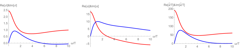
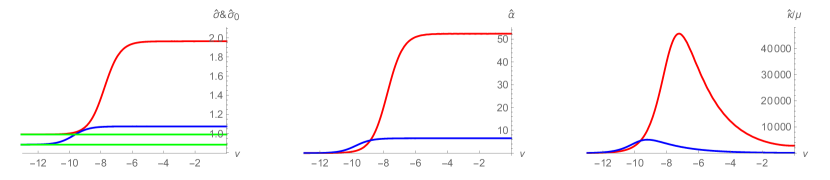
Now we can implement the numerical calculation and plot the AC thermo-electric conductivities. We focus on the limit $r\rightarrow\infty$, see Figure 1. They are denoted by $\left(\sigma,\alpha,\bar{\kappa}\right)$. The results are same to Ref. [23]. Note that we fix $r_{+}=1$ in all numerical calculations of this paper.

Figure 1: AC thermo-electric conductivities in the EMA model. The red and blue curves denote real and imaginary parts, respectively. We plot $\left(\hat{\sigma},\hat{\alpha},\hat{\kappa}\right)$ as the functions of $\omega/T$ on the boundary $r_{+}/r=10^{-4}$. We fix the dimensionless parameters $\mu/T=6$ and $\beta/T=5$ in order to compare with the green curves given in Figure 2 and Figure 8 in Ref. [23].

4 RG flow of ZHC conductivity in the DC limit

It is direct to show numerically that the RG flow of ZHC conductivity does not run in the DC limit. This is what we will do in the following for various holographic models. In Appendix B, we will present an alternative semi-analytical method. As a bonus, we will obtain the analytical expression of the contact term.

4.1 Einstein-Maxwell-axion model

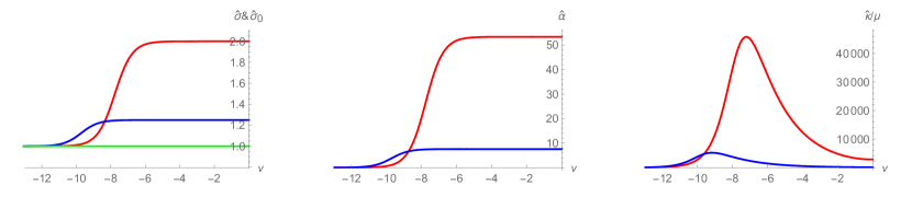
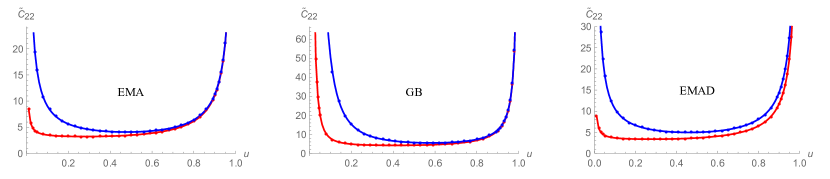
In Figure 2, we plot the trivial line that describes $\hat{\sigma}_{0}(r)$ and compare it with the nontrivial RG flow of three thermo-electric conductivities. It is amazing that the nontrivial evolution of $\left(\hat{\sigma},\hat{\alpha},\hat{\kappa}\right)$ exactly cancels each other to produce $\hat{\sigma}_{0}(r)=\mathrm{const}$.

Figure 2: $\left(\hat{\sigma},\hat{\alpha},\hat{\kappa}\right)$ and $\hat{\sigma}_{\mathrm{0}}$ as the functions of $v=\log(1-r_{+}/r)$ at $\omega/\mu=10^{-4}$ in the EMA model. The coordinate $v$ is used to highlight the near-horizon behavior. For $\left(\hat{\sigma},\hat{\alpha},\hat{\kappa}\right)$, we fix the parameters $T/\mu=1$ and $\beta/\mu=1$ (red), or $T/\mu=1/2$ and $\beta/\mu=2$ (blue). The green lines depict $\hat{\sigma}_{\mathrm{0}}$ for both groups of parameters. They merge in the EMA model. But it is not the case for other models.

4.2 Gauss-Bonnet curvature

The higher derivative corrections appear generally in any quantum gravity theory from quantum or stringy effects. These corrections may be holographic dual to $1/N$ or $1/\lambda$ corrections in some gauge theories, allowing independent values of two central charges $a$ and $c$. This is in contrast to the standard $\mathcal{N}$=4 super Yang-Mills theory where $a=c$. Actually, the Gauss-Bonnet (GB) correction has been treated as a dangerous source of violation for the feature that is universal in the Einstein gravity [39]. In the following, we will use GB gravity as a good test for the universality of RG flow.

Consider the GB correction to the EMA theory, with the bulk action [40, 41, 42, 43]

$$S_{\mathrm{bulk}} = \int d^{5}x\sqrt{-g}\big{[}R+12-\frac{1}{4}F^{\mu\nu}F_{\mu\nu}-\frac{1}{2}\sum\limits_{i=1}^{3}\left(\partial\chi_{i}\right)^{2}$$ (37)

$$+\frac{\tilde{\alpha}}{2}\left(R^{2}-4R^{\mu\nu}R_{\mu\nu}+R_{\mu\nu\lambda\rho}R^{\mu\nu\lambda\rho}\right)\big{]},$$

where $\tilde{\alpha}$ is the GB coupling constant. The isotropic black-brane solution can be written as [43]

$$ds^{2} = -h(r)dt^{2}+\frac{1}{f(r)}dr^{2}+r^{2}(dx_{1}^{2}+dx_{2}^{2}+dx_{3}^{2}),$$

$$f(r) = \frac{r^{2}}{2\tilde{\alpha}}\left[1-\sqrt{1+\tilde{\alpha}\frac{2\left(r^{2}-r_{+}^{2}\right)}{3r^{6}r_{+}^{2}}\left[q^{2}+3r^{2}r_{+}^{2}\left(\beta^{2}-4r^{2}-4r_{+}^{2}\right)\right]}\right],$$

$$h(r) = L_{\mathrm{eff}}^{2}f(r),\;A=\frac{L_{\mathrm{eff}}q}{2r_{+}^{2}}(1-\frac{r_{+}^{2}}{r^{2}})dt,\;\chi_{i}=\beta x_{i},\;i=1,2,3.$$ (38)

Here $L_{\mathrm{eff}}^{2}=\frac{1+\sqrt{1-4\tilde{\alpha}}}{2}$ is the square of the effective AdS radius. In contrast to the GB metric that is usually used in the literature, we have rescaled $t\rightarrow tL_{\mathrm{eff}}$. Thus, the RG flow that we will construct can match on the boundary to the AdS/CFT result. For instance, the observed temperature is $\hat{T}\left(r\right)=\frac{r}{\sqrt{h(r)}}T$, which can be directly reduced to the Hawking temperature $T$ at $r\rightarrow\infty$ due to our rescaling of time. The temperature and charge density can be written as

$$T=\frac{L_{\mathrm{eff}}}{\pi}\left(r_{+}-\frac{\beta^{2}}{8r_{+}}-\frac{q^{2}}{24r_{+}^{5}}\right),\;q=2r_{+}^{2}\frac{\mu}{L_{\mathrm{eff}}}.$$ (39)

Consider the relevant modes along $x=x_{1}$ direction, which are given by

$$\delta g_{tx}=r^{2}h_{tx}(r)e^{-i\omega t},\;\delta A_{x}=a_{x}(r)e^{-i\omega t},\;\delta\chi_{1}=\beta^{-1}\chi\left(r\right)e^{-i\omega t}.$$ (40)

Define an auxiliary transport matrix $\tau$ by

$$\left(\begin{array}[]{c}-r\sqrt{hf}a_{x}^{\prime}\\ -r^{-3}\sqrt{hf}\psi^{\prime}\end{array}\right)=\left(\begin{array}[]{cc}\tau_{11}&\tau_{12}\\ \tau_{21}&\tau_{22}\end{array}\right)\left(\begin{array}[]{c}i\omega a_{x}\\ i\omega\psi\end{array}\right),$$ (41)

where $\psi=r^{3}\sqrt{hf}\chi^{\prime}/\omega$. From three EOM

$$\left(qh_{tx}+r\sqrt{fh}a_{x}^{\prime}\right)^{\prime}+\frac{r}{\sqrt{fh}}\omega^{2}a_{x} = 0,$$

$$\chi^{\prime}-\frac{i\omega}{h}\left[\left(r^{2}-2\tilde{\alpha}f\right)h_{tx}^{\prime}+A_{t}^{\prime}a_{x}\right] = 0,$$

$$\left(r^{3}\sqrt{fh}\chi^{\prime}\right)^{\prime}+\frac{\omega r^{3}}{\sqrt{fh}}\left(\omega\chi-i\beta^{2}h_{tx}\right) = 0,$$ (42)

one can construct a matrix-form Riccati equation

$$\tau^{\prime}=\frac{1}{i\omega}A+i\omega\tau B\tau,$$ (43)

where the matrix $A$ and $B$ are

$$A=\frac{1}{r^{3}\sqrt{fh}}\left(\begin{array}[]{cc}r^{4}\omega^{2}-\frac{q^{2}h}{r^{2}-2\tilde{\alpha}f}&-\frac{iqh}{r^{2}-2\tilde{\alpha}f}\\ \frac{iq\beta^{2}h}{r^{2}-2\tilde{\alpha}f}&\omega^{2}-\frac{\beta^{2}h}{r^{2}-2\tilde{\alpha}f}\end{array}\right),\;B=\frac{1}{r\sqrt{fh}}\left(\begin{array}[]{cc}1&0\\ 0&r^{4}\end{array}\right).$$ (44)

Applying the regularity of $\tau$ on the horizon, one can extract the horizon value of $\tau$ from Eq. (43) directly:

$$\tau(r_{+})=\left(\begin{array}[]{cc}r_{+}&0\\ 0&r_{+}^{-3}\end{array}\right).$$ (45)

Using $\tau(r_{+})$ as the boundary condition, we can integrate out the RG flow $\tau(r)$.

To obtain the positioned on-shell action $S_{\mathrm{os}}$, we need the Gibbons-Hawking term and the counterterm [40, 41, 42, 43]

$$S_{\mathrm{GH}} = -2\int d^{4}x\sqrt{-\gamma}K,$$ (46)

$$S_{\mathrm{ct}} = \int d^{4}x\sqrt{-\gamma}\left(-6+\frac{1}{2}\sum\limits_{i=1}^{3}\gamma^{ab}\partial_{a}\chi_{i}\partial_{b}\chi_{i}\right).$$ (47)

Taking the variation of $S_{\mathrm{os}}$, one can calculate the one-point functions

$$\frac{\delta S_{\mathrm{os}}}{\delta a_{x}} = -qh_{tx}-r\sqrt{fh}a_{x}^{\prime},$$

$$\frac{\delta S_{\mathrm{os}}}{\delta h_{tx}} = r^{3}\sqrt{\frac{f}{h}}\left(r^{2}-2\tilde{\alpha}f\right)h_{tx}^{\prime}+\bar{C}_{22}h_{tx},$$ (48)

where we have neglected some terms that do not contribute to the DC conductivities. The function $\bar{C}_{22}$ is given by

$$\bar{C}_{22}=\frac{r^{2}}{4L_{\mathrm{eff}}\sqrt{h}}\left[\beta^{2}L_{\mathrm{eff}}^{2}r-8r^{3}\left(2+\sqrt{1-4\tilde{\alpha}}\right)+8L_{\mathrm{eff}}\sqrt{f}\left(3r^{2}-2\tilde{\alpha}f\right)\right].$$ (49)

Applying Eq. (41) and Eq. (42) to eliminate the derivatives of sources in Eq. (48), we can obtain

$$G_{11} = i\omega\left(\tau_{11}-\frac{\tau_{12}\tau_{21}}{\tau_{22}}\right),\;G_{12}=-\left(i\beta^{2}\frac{\tau_{12}}{\tau_{22}}+q\right),$$

$$G_{21} = \frac{i\tau_{21}}{\tau_{22}}-q,\;G_{22}=\bar{C}_{22}+\frac{i\beta^{2}}{\omega\tau_{22}}.$$ (50)

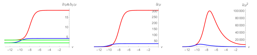
Interestingly, they have the same form as Eq. (35), up to $\bar{C}_{22}$. Inserting them into Eq. (15) and Eq. (18), $\left(\hat{\sigma},\hat{\alpha},\hat{\kappa}\right)$ and $\hat{\sigma}_{\mathrm{0}}$ can be inferred from $\tau$. We plot their RG flow in Figure 3.

Figure 3: The RG flow of $\left(\hat{\sigma},\hat{\alpha},\hat{\kappa}\right)$ and $\hat{\sigma}_{\mathrm{0}}$ in the GB model. The coupling constant is $\tilde{\alpha}=9/100$. In this and other remaining figures, the parameters $T$ and $\beta$ and the color scheme are same as those in Figure 2.

4.3 Dilaton field

Adding the dilaton is natural from the dimensional reductions of consistent string theory. In the AdS/CMT duality, the dilaton theory is particularly appealing as it provides various distinctive physical properties [49]. We will consider an Einstein-Maxwell-Axion-Dilaton (EMAD) theory. Its bulk action is given by

$$S_{\mathrm{bulk}}=\int d^{4}x\sqrt{-g}{\bigg{[}}R-\frac{Z\left(\phi\right)}{4}F^{\mu\nu}F_{\mu\nu}-\frac{1}{2}\nabla_{\mu}\chi_{i}\nabla^{\mu}\chi_{i}-\frac{1}{2}\nabla_{\mu}\phi\nabla^{\mu}\phi+V\left(\phi\right){\bigg{]}},$$ (51)

where the gauge field coupling and the scalar potential are taken as [50],

$$Z\left(\phi\right)=\exp(\phi/\sqrt{3}),\;V\left(\phi\right)=6\cosh(\phi/\sqrt{3}).$$ (52)

In Ref. [51], the Einstein-Maxwell-Dilaton theory with the massive graviton has been studied. Using Eq. (52), the analytical black brane solution has been found. We notice that there is a similar black brane solution in the EMAD theory

$$ds^{2} = r^{2}f(r)\left(-h(r)dt^{2}+dx^{2}+dy^{2}\right)+\frac{1}{r^{2}f(r)h(r)}dr^{2},$$ (53)

$$h(r) = 1-\frac{1}{\left(Q+r\right)^{3}}\left(m+Q^{3}+\frac{\beta^{2}r}{2}\right),\;f(r)=\left(1+\frac{Q}{r}\right)^{\frac{3}{2}}$$

$$A = \frac{\sqrt{3Q\left(m+Q^{3}-\frac{\beta^{2}}{2}\right)}}{Q+r_{+}}\frac{r-r_{+}}{Q+r}dt,\;\phi(r)=\frac{\sqrt{3}}{2}\log\left(1+\frac{Q}{r}\right),\;\chi_{i}=\beta x_{i},$$

where $m$ and $Q$ are two parameters. The temperature, chemical potential, and charge density can be written as

$$T=\frac{\sqrt{r_{+}}\left[6\left(Q+r_{+}\right)^{2}-\beta^{2}\right]}{8\pi\left(Q+r_{+}\right)^{3/2}},\;\mu=\frac{q}{Q+r_{+}},\;q=\frac{\sqrt{3Q\left(m+Q^{3}-\frac{\beta^{2}}{2}\right)}}{Q+r_{+}}.$$ (54)

Next, we will derive the EOM of vector modes and build up the Riccati equation. Note that a general EMAD model would allow various background solutions. For the potential application in the future, we will set a general metric ansatz

$$ds^{2}=g_{tt}\left(r\right)dt^{2}+g_{rr}\left(r\right)dt^{2}+g_{xx}\left(r\right)\left(dx^{2}+dy^{2}\right).$$ (55)

Consider the perturbation modes

$$\delta g_{tx}=g_{xx}\left(r\right)h_{tx}(r)e^{-i\omega t},\;\delta A_{x}=a_{x}(r)e^{-i\omega t},\;\delta\chi_{1}=\beta^{-1}\chi\left(r\right)e^{-i\omega t}.$$ (56)

The relevant EOM are

$$\left(qh_{tx}+\sqrt{-\frac{g_{tt}}{g_{rr}}}Za_{x}^{\prime}\right)^{\prime}+\sqrt{-\frac{g_{rr}}{g_{tt}}}\omega^{2}Za_{x} = 0,$$

$$\left(\sqrt{-\frac{g_{tt}}{g_{rr}}}g_{xx}\chi^{\prime}\right)^{\prime}-i\omega\sqrt{-\frac{g_{rr}}{g_{tt}}}g_{xx}\left(\beta^{2}h_{tx}+i\omega\chi\right) = 0,$$

$$\chi^{\prime}+i\omega\left(\frac{g_{xx}}{g_{tt}}h_{tx}^{\prime}-\sqrt{-\frac{g_{rr}}{g_{tt}}}\frac{1}{g_{xx}}qa_{x}\right) = 0.$$ (57)

They imply a matrix-form Riccati equation

$$\tau^{\prime}=\frac{1}{i\omega}A+i\omega\tau B\tau,$$ (58)

where the $\tau$ matrix is defined by

$$\left(\begin{array}[]{c}-\sqrt{-\frac{g_{tt}}{g_{rr}}}Za_{x}^{\prime}\\ -\sqrt{-\frac{g_{tt}}{g_{rr}}}\frac{1}{g_{xx}}\psi^{\prime}\end{array}\right)=\left(\begin{array}[]{cc}\tau_{11}&\tau_{12}\\ \tau_{21}&\tau_{22}\end{array}\right)\left(\begin{array}[]{c}i\omega a_{x}\\ i\omega\psi\end{array}\right),$$ (59)

and

$$A=\frac{\sqrt{-g_{tt}g_{rr}}}{g_{xx}^{2}}\left(\begin{array}[]{cc}-q^{2}-\frac{g_{xx}^{2}}{g_{tt}}Z\omega^{2}&-iq\\ i\beta^{2}q&-\beta^{2}-\frac{g_{xx}}{g_{tt}}\omega^{2}\end{array}\right),\;B=\sqrt{-\frac{g_{rr}}{g_{tt}}}\left(\begin{array}[]{cc}\frac{1}{Z}&0\\ 0&g_{xx}\end{array}\right).$$ (60)

On the horizon, the regularity of $\tau$ induces

$$\tau(r_{+})=\left.\left(\begin{array}[]{cc}Z&0\\ 0&\frac{1}{g_{xx}}\end{array}\right)\right|_{r=r_{+}}.$$ (61)

The holographic renormalization of the Einstein-Maxwell-Dilaton model given in [50] has been studied recently in [52]. Adding the axions does not lead to qualitative differences. Then we can read off the counterterm

$$S_{\mathrm{ct}}=\int d^{3}x\sqrt{-\gamma}\left(-4+\frac{1}{2}\sum\limits_{i=1}^{2}\gamma^{ab}\partial_{a}\chi_{i}\partial_{b}\chi_{i}+\frac{1}{3}\phi n^{r}\partial_{r}\phi-\frac{1}{6}\phi^{2}\right),$$ (62)

where $n^{r}$ is the radial component of the outward unit vector normal to the cutoff surface. Note that the Gibbons-Hawking term is same to one in the EMA theory. As a result, we can derive the one-point functions

$$\frac{\delta S_{\mathrm{os}}}{\delta a_{x}} = -qh_{tx}-Z\sqrt{\frac{-g_{tt}}{g_{rr}}}a_{x}^{\prime},$$

$$\frac{\delta S_{\mathrm{os}}}{\delta h_{tx}} = g_{xx}^{2}\frac{1}{\sqrt{-g_{tt}g_{rr}}}h_{tx}^{\prime}+\bar{C}_{22}h_{tx},$$ (63)

where

$$\bar{C}_{22}=\frac{\partial_{r}g_{xx}^{2}}{\sqrt{-g_{tt}g_{rr}}}-\frac{g_{xx}^{2}}{\sqrt{-g_{tt}}}\left(4+\frac{\phi^{2}}{6}+\frac{\phi\phi^{\prime}}{3\sqrt{g_{rr}}}\right).$$ (64)

Applying Eq. (57) and Eq. (59) to eliminate the derivatives of sources in Eq. (63), we can obtain

$$G_{11} = i\omega\left(\tau_{11}-\frac{\tau_{12}\tau_{21}}{\tau_{22}}\right),\;G_{12}=-\left(i\beta^{2}\frac{\tau_{12}}{\tau_{22}}+q\right),$$

$$G_{21} = \left(\frac{i\tau_{21}}{\tau_{22}}-q\right),\;G_{22}=\bar{C}_{22}+\frac{i\beta^{2}}{\omega\tau_{22}},$$ (65)

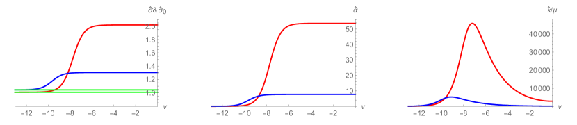
which are still same to Eq. (35), up to $\bar{C}_{22}$. Inserting them into Eq. (15) and Eq. (18), we can deduce $\left(\hat{\sigma},\hat{\alpha},\hat{\kappa}\right)$ and $\hat{\sigma}_{\mathrm{0}}$ from $\tau$. Their RG flow is depicted in Figure 4.

Figure 4: The RG flow of $\left(\hat{\sigma},\hat{\alpha},\hat{\kappa}\right)$ and $\hat{\sigma}_{\mathrm{0}}$ in the EMAD model.

4.4 Non-minimal coupling

In all of the above models, the translation-breaking sector is minimally coupled to the gravitational and electromagnetic sectors. There are novel models which involve the non-minimal coupling between the Maxwell term and the axions [53, 54, 55]. We will focus on one of these models, i.e. the model 1 in [54], which has more nontrivial conductivities than others. This model is so distinctive that it breaks various bounds on the viscosity [56], electric conductivity [57] and charge diffusivity [58]. The action is given by

$$S_{\mathrm{bulk}}=\int d^{4}x\sqrt{-g}\left(R+6-\frac{1}{4}F^{2}-\frac{1}{4}\mathcal{J}\mathrm{Tr}\left[\mathcal{X}F^{2}\right]-\mathrm{Tr}\left[\mathcal{X}\right]\right),$$ (66)

where the coupling constant belongs to $0\mathcal{\leq J\leq}2/3$ by the causality requirement and

$$\mathcal{X}_{\;\nu}^{\mu}=\frac{1}{2}\sum\limits_{i=1}^{2}\partial^{\mu}\chi_{i}\partial_{\nu}\chi_{i}.$$ (67)

The background solution is same as Eq. (21). Suppose that the background is perturbed by the vector mode along $x=x_{1}$:

$$\delta g_{tx}=r^{2}h_{tx}(r)e^{-i\omega t},\;\delta A_{x}=a_{x}(r)e^{-i\omega t},\;\delta\chi=\beta^{-1}\chi\left(r\right)e^{-i\omega t}.$$ (68)

Due to the non-minimal coupling, the number of the relevant EOM is not three but four:

$$\left(qh_{tx}+ha_{x}^{\prime}\right)^{\prime}+\frac{\omega^{2}}{h}a_{x}+\frac{2\mathcal{J}}{r(4r^{2}-\mathcal{J}\beta^{2})}\left[\beta^{2}\left(qh_{tx}+ha_{x}^{\prime}\right)+i\omega q\chi\right] = 0,$$

$$\left(r^{2}h\chi^{\prime}\right)^{\prime}-\frac{i\omega r^{2}}{h}\left(\beta^{2}h_{tx}+i\omega\chi\right)-\frac{2\mathcal{J}qr}{4r^{4}+\mathcal{J}q^{2}}\left(i\omega\beta^{2}a_{x}+2qh\chi^{\prime}\right) = 0,$$

$$\left(r^{4}h_{tx}^{\prime}+qa_{x}\right)^{\prime}-\frac{r^{2}}{h}\left(\beta^{2}h_{tx}+i\omega\chi\right)-\frac{\mathcal{J}q}{4r^{2}h}\left[\beta^{2}\left(qh_{tx}+ha_{x}^{\prime}\right)+i\omega q\chi\right] = 0,$$

$$\chi^{\prime}-\frac{i\omega}{r^{2}h}\left(qa_{x}+r^{4}h_{tx}^{\prime}\right)+\frac{i\omega\mathcal{J}q}{r^{2}h\left(4r^{4}+\mathcal{J}q^{2}\right)}\left[q\left(qa_{x}+r^{4}h_{tx}^{\prime}\right)+\beta^{2}r^{2}a_{x}\right] = 0.$$ (69)

To deal with these EOM, we define a $3\times 3$ auxiliary transport matrix $\tau$ by

$$\left(\begin{array}[]{c}-\frac{4r^{2}-\mathcal{J}\beta^{2}}{4r^{2}}ha_{x}^{\prime}\\ r^{4}h_{tx}^{\prime}\\ -r^{2}h\chi^{\prime}\end{array}\right)=\left(\begin{array}[]{ccc}\tau_{11}&\tau_{12}&\tau_{12}\\ \tau_{21}&\tau_{22}&\tau_{23}\\ \tau_{13}&\tau_{23}&\tau_{33}\end{array}\right)\left(\begin{array}[]{c}i\omega a_{x}\\ i\omega h_{tx}\\ i\omega\chi\end{array}\right).$$ (70)

The former three EOM can be recast as

$$\tau^{\prime}=\frac{1}{i\omega}A+i\omega\tau B\tau+C\tau,$$ (71)

where

$$A = \frac{1}{h}\left(\begin{array}[]{ccc}\frac{4r^{2}-\mathcal{J}\beta^{2}}{4r^{2}}\omega^{2}&\frac{\mathcal{J}\beta^{2}qh}{2r^{3}}&\frac{i\omega\mathcal{J}qh}{2r^{3}}\\ 0&\frac{4r^{4}+\mathcal{J}q^{2}}{4r^{2}}\beta^{2}&i\omega\frac{4r^{4}+\mathcal{J}q^{2}}{4r^{2}}\\ -\frac{2i\omega\mathcal{J}\beta^{2}qrh}{4r^{4}+\mathcal{J}q^{2}}&-i\omega\beta^{2}r^{2}&r^{2}\omega^{2}\end{array}\right),$$ (75)

$$B = \frac{1}{h}\left(\begin{array}[]{ccc}\frac{4r^{2}}{4r^{2}-\mathcal{J}\beta^{2}}&0&0\\ 0&-\frac{h}{r^{4}}&0\\ 0&0&\frac{1}{r^{2}}\end{array}\right),\;C=\frac{q}{r^{4}}\left(\begin{array}[]{ccc}0&\frac{4r^{2}-\mathcal{J}\beta^{2}}{4r^{2}}&0\\ \frac{r^{4}}{h}&0&0\\ 0&0&\frac{4\mathcal{J}qr^{3}}{4r^{4}+\mathcal{J}q^{2}}\end{array}\right).$$ (82)

The regularity on the horizon gives

$$\tau(r_{+})=\left(\begin{array}[]{ccc}\frac{4r^{2}-\mathcal{J}\beta^{2}}{4r^{2}}&0&0\\ \frac{iq}{\omega}\frac{4r^{2}-\mathcal{J}\beta^{2}}{4r^{2}}&\tau_{22}(r)&\frac{i}{\omega}\frac{4r^{4}+\mathcal{J}q^{2}}{4r^{2}}\\ 0&\frac{\beta^{2}r^{2}}{i\omega}&r^{2}\end{array}\right)_{r=r_{+}}.$$ (83)

To determine $\tau_{22}(r_{+})$, one can rely on the last line of Eq. (69), which leads to the constraint

$$\left(\begin{array}[]{ccc}0&0&0\\ 0&0&0\\ 0&i\omega\frac{4r^{4}}{4r^{4}+\mathcal{J}q^{2}}&0\end{array}\right)\left(\begin{array}[]{ccc}\tau_{11}&\tau_{12}&\tau_{12}\\ \tau_{21}&\tau_{22}&\tau_{23}\\ \tau_{13}&\tau_{32}&\tau_{33}\end{array}\right)=\left(\begin{array}[]{ccc}0&0&0\\ 0&0&0\\ -qr^{2}\frac{4r^{2}-\mathcal{J}\beta^{2}}{4r^{4}+\mathcal{J}q^{2}}&0&0\end{array}\right).$$ (84)

Combining the above two equations, one can obtain

$$\tau_{22}(r_{+})=\frac{i}{\omega}\frac{4r_{+}^{4}+\mathcal{J}q^{2}}{4r_{+}^{4}}\tau_{32}(r_{+}).$$ (85)

Using the bulk action (66), the Gibbons-Hawking term (31) and the counter term (32), we calculate the one-point functions

$$\frac{\delta S_{\mathrm{os}}}{\delta a_{x}} = -\frac{4r^{2}-\mathcal{J}\beta^{2}}{4r^{2}}\left(qh_{tx}+ha_{x}^{\prime}\right),$$

$$\frac{\delta S_{\mathrm{os}}}{\delta h_{tx}} = \bar{C}_{22}h_{tx}+r^{4}h_{tx}^{\prime},$$ (86)

where $\bar{C}_{22}$ is same to Eq. (34). Substituting Eq. (70) into Eq. (86), one can extract

$$G_{11} = i\omega\tau_{11},\;G_{12}=i\omega\tau_{12}-q\frac{4r^{2}-\mathcal{J}\beta^{2}}{4r^{2}},$$

$$G_{21} = i\omega\tau_{21},\;G_{22}=\bar{C}_{22}+i\omega\tau_{22}.$$ (87)

Inserting them into Eq. (15) and Eq. (18), we can deduce $\left(\hat{\sigma},\hat{\alpha},\hat{\kappa}\right)$ and $\hat{\sigma}_{\mathrm{0}}$ from $\tau$. Their RG flow is depicted in Figure 5.

Figure 5: The RG flow of $\left(\hat{\sigma},\hat{\alpha},\hat{\kappa}\right)$ and $\hat{\sigma}_{\mathrm{0}}$ in the theory with the non-minimal coupling $\mathcal{J=}2/3$.

5 Analytical DC thermal conductivity

We have exhibited a trivial RG flow $\hat{\sigma}_{0}\left(r\right)=\hat{\sigma}_{0}\left(r_{+}\right)$. As a result, the DC thermal conductivity on the boundary can be expressed as

$$\bar{\kappa}=\frac{T\alpha^{2}}{\sigma-\hat{\sigma}_{0}\left(r_{+}\right)}.$$ (88)

We argue that this provides an analytical method to calculate $\bar{\kappa}$, if $\sigma$, $\alpha$, and $\hat{\sigma}_{0}\left(r_{+}\right)$ have been obtained analytically. The first two ($\sigma$, $\alpha$) can be derived in terms of the conserved electric current [28]. With the help of the regularity of the Riccati equation on the horizon, we can write down the analytical expression of the latter one $\hat{\sigma}_{0}\left(r_{+}\right)$ for all the models which have been studied. More simply, by observing the RG flow in above figures, one can find that the ZHC conductivity meets the electrical conductivity on the horizon. So let’s write down the expression of $\sigma_{\mathrm{H}}\equiv\hat{\sigma}(r_{+})$ in those models. Using the infrared boundary condition (30) and the relation between the electric conductivity and the auxiliary transport matrix (36), we can read $\sigma_{\mathrm{H}}=1$ for the EMA model. It is changed as $\sigma_{\mathrm{H}}=r_{+}$ for the GB gravity. The change comes from the increase of the spacetime dimension instead of the GB coupling. For the EMAD theory, one can see the effect from the gauge field coupling, $\sigma_{\mathrm{H}}=Z\left(r_{+}\right)$. For the theory with non-minimal coupling, $\sigma_{\mathrm{H}}=1-\mathcal{J}\beta^{2}/\left(4r_{+}^{2}\right)$. Combining the analytical expression of the electric conductivity on the horizon and the boundary thermo-electric conductivities that have been derived in [28, 43, 55], e.g., $\sigma=1+\frac{q^{2}}{r_{+}^{2}\beta^{2}},\;\alpha=\frac{4\pi q}{\beta^{2}},\;\bar{\kappa}=\frac{16\pi^{2}r_{+}^{2}T}{\beta^{2}}$ for the EMA model, one can check $\bar{\kappa}=T\alpha^{2}/\left(\sigma-\sigma_{\mathrm{H}}\right)$, as it should be.

6 Conclusion

We constructed a holographic RG flow of the thermo-electric transport in the strongly coupled systems with momentum dissipation. The essence of the RG flow is to reformulate the classical EOM in terms of the transport coefficients measured by the intrinsic observers on the sliding membranes. The reformulation involves two steps: recast the perturbation equations into a Riccati equation of an auxiliary transport matrix $\tau$ and then translate $\tau$ into the thermo-electric conductivities observed on the membranes.

The RG flow is useful for the field theory on the boundary. First, it provides a new method to calculate the AC thermo-electric conductivities. Compared with the traditional method that solves the second-order perturbation equations directly [23], the new method simplifies the numerical calculation by just solving the first-order nonlinear ordinary differential equation. Second, it can be used to derive the analytical expression of the DC thermal conductivity, provided that in the DC limit the RG flow of the ZHC conductivity does not run and the electric conductivity and thermoelectric conductivity have been obtained analytically. Compared with the well-known Donos-Gauntlett method [28], the RG flow method does not need to construct the thermal current that could be subtle.

Besides the application to the boundary, the RG flow itself is interesting. As we have shown, the RG flow of the ZHC conductivity in the DC limit does not run for some holographic models at finite density. This generalizes the well-known result of the membrane paradigm: the DC electrical conductivity for neutral black holes has the trivial flow [24]. We hope that our result might provide some hints for understanding the universal thermo-electric transport in various strongly correlated systems [59]. In particular, the $T$-linear resistivity in cuprate strange metals can persist from near $T_{c}$ up to as high a temperature as measured. The quick crossover from the microscopic chemistry to the macroscopic strange-metal physics near the “ultraviolet” temperature indicates one decimation along the RG flow in essence [60].

In the future, we would like to explore whether or not the trivial RG flow is universal when the holographic model is inhomogeneous and anisotropic.

Appendix A Thermodynamics on the membranes

Here we will present the observed thermodynamics on the membranes. We start from the positioned on-shell action. Analogue to the AdS/CFT, we define the observed grand potential by

$$\hat{\Omega}=-\hat{T}S_{\mathrm{os}},$$ (89)

where the Tolman temperature

$$\hat{T}\left(r_{c}\right)=T\frac{\Lambda(r_{c})}{\sqrt{-\gamma_{00}(r_{c})}}$$ (90)

has been invoked. We write the proper spatial volume as $\hat{V}=V_{0}\sqrt{\lambda_{d}}$, where $V_{0}$ denotes the spatial coordinate volume and will be set to one for convenience. The grand potential density gives the observed pressure $\hat{p}=-\hat{\Omega}/\hat{V}$. The observed chemical potential should be conjugate to the observed electric charge. Based on Eq. (9), it can be written as

$$\hat{\mu}=A_{\hat{t}}=A_{t}(r_{c})\frac{\Lambda(r_{c})}{\sqrt{-\gamma_{00}(r_{c})}}.$$ (91)

Also, one can see that the observed energy density is $\hat{\epsilon}\equiv T^{\hat{t}\hat{t}}$.

To be clear, we will apply the observed thermodynamics to the EMA model. The application to other models should be similar. Using the action (20), (31), and (32), we have found

$$\hat{p}=\Lambda^{3}\left[\frac{h^{\prime}}{\sqrt{h}}+\frac{2\sqrt{h}}{r_{c}}-4+\frac{\beta^{2}}{r_{c}^{2}}\left(1-\frac{r_{c}-r_{h}}{\sqrt{h}}\right)\right].$$ (92)

Using Eq. (90) and Eq. (91), one can express $\hat{p}$ as the function of $\hat{T}$ and $\hat{\mu}$. This can further induce

$$\left(\partial_{\hat{T}}\hat{p}\right)_{\hat{\mu}}=\frac{\Lambda^{2}}{r_{c}^{2}}s,\;\left(\partial_{\hat{\mu}}\hat{p}\right)_{\hat{T}}=\frac{\Lambda^{2}}{r_{c}^{2}}q,$$ (93)

where $s=4\pi r_{+}^{2}$. Keeping in mind $\sqrt{\lambda_{d}}=r_{c}^{2}/\Lambda^{2}$ in the present, we can obtain the expected relation for the observed thermodynamics:

$$\left(\partial_{\hat{T}}\hat{p}\right)_{\hat{\mu}}=\hat{s},\;\left(\partial_{\hat{\mu}}\hat{p}\right)_{\hat{T}}=\hat{q},$$ (94)

where $\hat{s}=s/\sqrt{\lambda_{d}}$ and $\hat{q}=q/\sqrt{\lambda_{d}}$ are the observed entropy density and charge density, respectively. In particular, it implies that the total entropy $S\equiv\hat{s}\hat{V}$ is conserved along the flow. This result recovers the assumption (the radial variation is isentropic) proposed in Ref. [30]. Furthermore, by calculating the observed energy density

$$\hat{\epsilon}=\Lambda^{3}\left(4-4\frac{\sqrt{h}}{r_{c}}-\frac{\beta^{2}}{r_{c}^{2}}\right)$$ (95)

and collecting all the observed thermodynamic quantities above, one can also establish the Euler relation

$$\hat{\epsilon}+\hat{p}=\hat{T}\hat{s}+\hat{\mu}\hat{q}.$$ (96)

Note that the consistency of the observed thermodynamics does not depend on the choice of the conformal factor $\Lambda^{2}$.

Appendix B Semi-analytical proof

Here we will verify semi-analytically

$$\partial_{r}\hat{\sigma}_{\mathrm{0}}=\mathcal{O}\left(\omega\right).$$ (97)

It is based on an assumption: up to the pole from the contact term $C_{22}$, the canonical response functions $\Gamma_{IJ}\equiv G_{IJ}/\left(i\omega\right)$ are finite in the DC limit. The assumption can be justified using the numerical method.

Let’s illustrate Eq. (97) in the simplest EMA model. We have to translate the non-canonical response functions $\tau$ into the canonical response functions $\Gamma$. However, it is difficult to inverse Eq. (35) since it is nonlinear. Therefore, we adopt Eq. (87) with $\mathcal{J}=0$ by which $\tau$ can be represented by $G$ readily. Then the canonical response functions can be read from $\Gamma=\frac{1}{i\omega}G$. To subtract the pole in $\Gamma$, we define

$$\tilde{\Gamma}_{22}=\frac{1}{i\omega}\left(G_{22}-C_{22}\right),$$ (98)

which is finite at $\omega\rightarrow 0$ and will be used to replace $\Gamma_{22}$ in the calculation below.

Putting Eqs. (15), (71), (87), and (98) together, we can derive

$$\partial_{r}\hat{\sigma}_{\mathrm{0}}=\frac{F_{1}(\Gamma)}{i\omega}\left[r^{4}\left(q^{2}+\beta^{2}r^{2}-h\tilde{C}_{22}^{\prime}\right)-\tilde{C}_{22}^{2}h\right]+F_{2}(\Gamma)\left[\left(2r^{3}+\tilde{C}_{22}\right)h-r^{4}h^{\prime}\right]+\mathcal{O}(\omega),$$ (99)

where $\tilde{C}_{22}\equiv C_{22}-\bar{C}_{22}$ denotes the rest of the contact term, and

$$F_{1}(\Gamma) = -\frac{\left(r^{2}A_{t}\Gamma_{11}-\Gamma_{12}h\right)^{2}}{r^{4}\left[r^{4}A_{t}^{2}\Gamma_{11}-r^{2}A_{t}\left(\Gamma_{12}+\Gamma_{21}\right)h+\tilde{\Gamma}_{22}h^{2}\right]^{2}},$$ (100)

$$F_{2}(\Gamma) = \frac{A_{t}\left(r^{2}A_{t}\Gamma_{11}-\Gamma_{12}h\right)\left[r^{2}A_{t}\Gamma_{11}\left(\Gamma_{12}-\Gamma_{21}\right)-\Gamma_{12}\left(\Gamma_{12}+\Gamma_{21}\right)h-2\Gamma_{11}\tilde{\Gamma}_{22}\right]}{r^{2}\left[r^{4}A_{t}^{2}\Gamma_{11}-r^{2}A_{t}\left(\Gamma_{12}+\Gamma_{21}\right)h+\tilde{\Gamma}_{22}h^{2}\right]^{2}}.$$

Using the EOM for background fields $h$ and $A_{t}$, one can find that both terms in Eq. (99) vanish if

$$C_{22}=\bar{C}_{22}+r^{3}\left(\frac{rh^{\prime}}{h}-2\right).$$ (101)

In the left panel of Figure 6, we have checked numerically that Eq. (101) is the contact term $G_{22}\left(0\right)$ indeed. Thus, we have demonstrated Eq. (97) by a semi-analytical method. As a bonus, we have obtained the analytical expression of the contact term. To be more clear, we input Eq. (34) into Eq. (101). Then the contact term is

$$C_{22}=2r^{3}\left(1-\frac{r}{\sqrt{h}}+\frac{rh^{\prime}}{2h}\right).$$ (102)

On the boundary, one can find

$$C_{22}\left(r\rightarrow\infty\right)=\epsilon/2,$$ (103)

where $\epsilon$ is the energy density. The relation (103) has been obtained previously using the conserved current and the sources that are linear in time [28]. Alternatively, it can be derived in terms of Ward identities [61, 62], if other correlators have been known. This result can be taken as a self-consistent check of our theory.

Figure 6: $\tilde{C}_{22}$ as the functions of $u=r_{+}/r$ at $\omega/\mu=10^{-4}$ for three models. The GB coupling is fixed as $\tilde{\alpha}=9/100$. The curves denote the numerical functions $\tilde{C}_{22}=\lim_{\omega\rightarrow 0}G_{22}-\bar{C}_{22}$ and the points denote the analytical expressions.

The semi-analytical method also works for other theories. To avoid the repetition, we neglect the details of the derivation but only give the results. For the GB gravity, the contact term is

$$C_{22}=\bar{C}_{22}+r^{2}\sqrt{\frac{f}{h}}\left(r^{2}-4\alpha f\right)\left(\frac{rh^{\prime}}{h}-2\right).$$ (104)

For the EMAD theory with the metric ansatz (53), the contact term can be written as

$$C_{22}=\bar{C}_{22}+r^{4}f^{2}\frac{h^{\prime}}{h}.$$ (105)

They are both consistent with the numerical results, see the middle and right panels in Figure 6. On the boundary, one can check that they are equal to $\epsilon/3$ and $\epsilon/2$, respectively. At last, note that the non-minimal coupling does not change the contact term (102).

References

- [1] J. Zaanen, Y. W. Sun, and Y. Liu, Holographic duality in condensed matter physics, (CUP, 2015), Section 1.3.
- [2] K. G. Wilson and J. Kogut, Phys. Rep. 12, 75 (1974).
- [3] K. G. Wilson, Rev. Mod. Phys, 55, 583 (1983).
- [4] J. Polchinski, Nucl. Phys. B 231, 269 (1984).
- [5] J. M. Maldacena, Adv. Theor. Math. Phys. 2, 231 (1998) [arXiv:hep-th/9711200].
- [6] S. S. Gubser, I. R. Klebanov, and A. M. Polyakov, Phys. Lett. B 428, 105 (1998) [arXiv:hep-th/9802109].
- [7] E. Witten, Adv. Theor. Math. Phys. 2, 253 (1998) [arXiv:hep-th/9802150].
- [8] L. Susskind and E. Witten, arXiv:hep-th/9805114.
- [9] A. W. Peet and J. Polchinski, Phys. Rev. D 59, 065011 (1999) [arXiv:hep-th/9809022].
- [10] E. T. Akhmedov, Phys. Lett. B 442, 152 (1998) [arXiv:hep-th/9806217].
- [11] E. Alvarez and C. Gomez, Nucl. Phys. B 541, 441 (1999) [arXiv:hep-th/9807226].
- [12] L. Girardello, M. Petrini, M. Porrati, and A. Zaffaroni, JHEP 9812, 022 (1998) [arXiv:hep-th/9810126].
- [13] J. Distler and F. Zamora, Adv. Theor. Math. Phys. 2, 1405 (1999) [arXiv:hep-th/9810206].
- [14] V. Balasubramanian and P. Kraus, Phys. Rev. Lett. 83, 3605 (1999) [arXiv:hep-th/9903190].
- [15] D. Freedman, S. Gubser, K. Pilch, and N. Warner, Adv. Theor. Math. Phys. 3, 363 (1999) [arXiv:hep-th/9904017].
- [16] J. de Boer, E. P. Verlinde, and H. L. Verlinde, JHEP 08, 003 (2000) [arXiv:hep-th/9912012].
- [17] J. de Boer, Fortsch. Phys. 49, 339 (2001) [arXiv:hep-th/0101026].
- [18] T. Andrade and B. Withers, JHEP 1405, 1405 (2014) [arXiv:1311.5157].
- [19] X. H. Ge, Y. Tian, S. Y. Wu, and S. F. Wu, JHEP 11, 128 (2016) [arXiv:1606.07905].
- [20] X. H. Ge, Y. Tian, S. Y. Wu, and S. F. Wu, Phys. Rev. D 96, 046015 (2017) [arXiv:1606.05959].
- [21] Y. Tian, X. H. Ge, and S. F. Wu, Phys. Rev. D 96, 046011 (2017) [arXiv:1702.05470].
- [22] Y. Matsuo, S. J. Sin, and Y. Zhou, JHEP 1201, 130 (2012) [arXiv:1109.2698].
- [23] K. Y. Kim, K. K. Kim, Y. Seo, and S. J. Sin, JHEP 12, 170 (2014) [arXiv:1409.8346].
- [24] N. Iqbal and Hong Liu, Phys. Rev. D 79, 025023 (2009) [arXiv:0809.3808].
- [25] K. S. Thorne, R. H. Price and D. A. Macdonald, Black holes: the membrane paradigm, Yale University Press, New Haven 1986.
- [26] M. Parikh and F. Wilczek, Phys. Rev. D 58, 064011 (1998) [arXiv:gr-qc/9712077].
- [27] M. Blake and D. Tong, Phys. Rev. D 88, 106004 (2013) [arXiv:1308.4970].
- [28] A. Donos and J. P. Gauntlett, JHEP 1411, 081 (2014) [arXiv:1406.4742].
- [29] H. S. Liu, H. Lu, and C. N. Pope, JHEP 09, 146 (2017) [arXiv:1708.02329].
- [30] I. Bredberg, C. Keeler, V. Lysov, and A. Strominger, JHEP 1103, 141 (2011) [arXiv:1006.1902].
- [31] D. Nickel and D. T. Son, New J. Phys. 13, 075010 (2011).
- [32] I. Heemskerk and J. Polchinski, JHEP 06, 031 (2011).
- [33] T. Faulkner, H. Liu and M. Rangamani, JHEP 08, 051 (2011) [arXiv:1010.4036].
- [34] S. J. Sin and Y. Zhou, JHEP 1105, 030 (2011) [arXiv:1102.4477].
- [35] D. T. Son and A. O. Starinets, JHEP 09, 42 (2002) [arXiv:hep-th/0205051].
- [36] G. Policastro, D. T. Son, and A. O. Starinets, [arXiv:hep-th/0210220]
- [37] S. A. Hartnoll, Class. Quant. Grav. 26, 224002 (2009) [arXiv:0903.3246].
- [38] Y. Tian, X .N. Wu, and H. Zhang, JHEP 1410, 170 (2014) [arXiv:1407.8273].
- [39] H. Liu and S. J. Suh, Phys. Rev. Lett. 112, 011601 (2014) [arXiv:1305.7244].
- [40] Y. Brihaye and E. Radu, JHEP 0809, 006 (2008) [arXiv:0806.1396].
- [41] D. Astefanesei, N. Banerjee, and S. Dutta, JHEP 0811, 070 (2008) [arXiv:0806.1334].
- [42] J. T. Liu, and W. A. Sabra, Class. Quant. Grav. 27, 175014 (2010) [arXiv:0807.1256].
- [43] L. Cheng, X. H. Ge, and Z. Y. Sun, JHEP 04, 135 (2015) [arXiv:1411.5452].
- [44] M. Brigante, H. Liu, R. C. Myers, S. Shenker, and S. Yaida, Phys. Rev. Lett. 100, 191601 (2008) [arXiv:0802.3318]; Phys. Rev. D 77, 126006 (2008) [arXiv:0712.0805]; A. Buchel and R. C. Myers, JHEP 08, 016 (2009) [arXiv:0906.2922].
- [45] D. M. Hofman and J. Maldacena, JHEP 05, 012 (2008) [arXiv:0803.1467]; D. M. Hofman, Nucl. Phys. B 823, 174 (2009) [arXiv:0907.1625]; J. de Boer, M. Kulaxizi, and A. Parnachev, JHEP 03, 087 (2010) [arXiv:0910.5347]; X. O. Camanho and J. D. Edelstein, JHEP 1004, 007 (2010) [arXiv:0911.3160].
- [46] X. O. Camanho, J. D. Edelstein, J. Maldacena, and A. Zhiboedov, JHEP 02, 020 (2016) [arXiv:1407.5597].
- [47] G. Papallo and H. S. Reall, JHEP 1511, 109 (2015) [arXiv:1508.05303].
- [48] Y. L. Wang and X. H. Ge, Phys. Rev. D 94, 066007 (2016) [arXiv:1605.07248].
- [49] C. Charmousis et al., JHEP 1011, 151 (2010) [arXiv:1005.4690].
- [50] S. S. Gubser and F. D. Rocha, Phys. Rev. D 81, 046001 (2010) [arXiv:0911.2898].
- [51] R. A. Davison, K. Schalm and J. Zaanen, Phys. Rev. B 89, 245116 (2014) [arXiv:1311.2451].
- [52] B. S. Kim, JHEP 1611, 044 (2016) [arXiv:1608.06252].
- [53] M. Baggioli and O. Pujolas, JHEP 01, 040 (2017) [arXiv:1601.07897].
- [54] B. Goutéraux, E. Kiritsis and W. J. Li, JHEP 04, 122 (2016) [arXiv:1602.01067].
- [55] M. Baggioli, B. Goutéraux, E. Kiritsis and W. J. Li, arXiv:1612.05500.
- [56] P. K. Kovtun, D. T. Son, and A. O. Starinets, Phys. Rev. Lett. 94, 111601 (2005) [arXiv:hep-th/0405231].
- [57] S. Grozdanov, A. Lucas, S. Sachdev, and K. Schalm, Phys. Rev. Lett. 115, 221601 (2015) [arXiv:1507.00003].
- [58] S. A. Hartnoll, Nat. Phys. 11, 54 (2015) [arXiv:1405.3651].
- [59] See a recent review: S. A. Hartnoll, A. Lucas, and S. Sachdev, arXiv:1612.07324.
- [60] B. Keimer, S. A. Kivelson, M. R. Norman, S. Uchida, and J. Zaanen, Nature 518, 179 (2015) [arXiv:1409.4673].
- [61] C. P. Herzog, J. Phys. A 42, 343001 (2009) [0904.1975].
- [62] K. Y. Kim, K. K. Kim, and M. Park, JHEP 10, 041 (2016) [arXiv:1604.06205].