Optimal paths on the road network as directed polymers

Abstract

We analyze the statistics of the shortest and fastest paths on the road network between randomly sampled end points. To a good approximation, these optimal paths are found to be directed in that their lengths (at large scales) are linearly proportional to the absolute distance between them. This motivates comparisons to universal features of directed polymers in random media. There are similarities in scalings of fluctuations in length/time and transverse wanderings, but also important distinctions in the scaling exponents, likely due to long-range correlations in geographic and man-made features. At short scales the optimal paths are not directed due to circuitous excursions governed by a fat-tailed (power-law) probability distribution.

Complex networks of nodes and links characterize a wide array of systems, ranging form biological examples such as neural nets of neurons and synapses in the brain or chemical reactions inside a cell, to social or transportation networks and the World Wide Web. Their connectivity in the abstract space of edges and vertices has been much studied, illuminating characteristics such as ‘small-world’ separation, scale-free connectivity and a high degree of clustering, which can be captured by simple models Watts98 ; Barabasi99 ; Albert02 ; Ravasz03 ; Newman03 . Comparatively, less is understood about the spatial organization of complex networks embedded in a Euclidean space, a very active area of research BarYam1 ; BarYam2 (see also Ref.Barthelemy11 for a review). The effect of geometry is especially relevant when the network is strongly constrained by the environment or when the “cost” to maintain edges increases significantly with their length (e.g. rivers Dodds00 , railways Sen03 or vascular networks Hunt16 ). The spatial structure of streets is another example that has been particularly studied to gain insight into organization and development of cities Cardillo06 ; Lammer06 ; Barthelemy08 .

Much relevant information about the shape of a network is obtained by studying the shortest paths between its nodes Newman03 . More generally, it is of practical importance to find and characterize paths that optimize a given cost function of interest. For example, in transportation networks, one may like to understand properties of paths that minimize travel time, distance, or the monetary cost to go between two points. An obvious application is in the development of efficient GPS routing algorithms that use prior information on optimal paths to perform better Geisberger08 . This problem is challenging as the optimal paths on transportation networks strongly depend on network connectivities shaped by various factors, from natural obstacles to historical development or differences in policy.

Figure 1: The location of the three regions considered. For simplicity and efficiency of our algorithm, they are chosen to be large rectangular areas (in latitude-longitude coordinates) without sea or ocean.

The model of directed polymers in random media (DPRM) Kardar87 ; HH95 explores a physically distinct but mathematically related problem. It is concerned with the statistics of a chain stretched between two points that minimizes its energy in a random environment characterized by a rough energy landscape. The optimal chain configuration is then governed by a trade-off between a line tension (preferring the straight polymer) and the hills and valleys of the random landscape which encourage its wanderings. A wealth of theoretical results is available for this widely studied problem, which belongs to the Kardar-Parisi-Zhang (KPZ) KPZ universality class (originally posed to describe roughening of growing surfaces).

Configurations of DPRM paths bear superficial resemblance to myriad natural transportation systems, from deltas of rivers to vascular networks; the wealth of data on road networks provides the opportunity for a quantitative comparison. Here, we study the statistics of optimal (shortest and fastest) paths on the road network in light of known statistics for DPRM. Gathering large data sets of millions of paths on three continents, we compute the probability distribution of path length and travel time as a function of the (straight-line) distance between the end points. As a preliminary step, we confirm that long optimal paths are directed in the sense that the average length/time of the path is (at large separations) linearly proportional to the straight-line distance. We next examine the fluctuations of the optimized quantity. As in the case of DPRM, appropriately scaled fluctuations can be collapsed (approximately) to a single curve, suggesting that details of the local structure of road networks are irrelevant to the statistics on larger scales. However, the scaling forms do not correspond to the simplest variant of DPRM with uncorrelated energies, indicating long-range correlations on the scale of hundred of kilometers. The transverse wanderings of the paths is also consistent with this picture. Remarkably, the distributions at short-scales are broad with a power-law tail of universal exponent that captures the profusion of long non-directed circuitous routes at separations of a few kilometers.

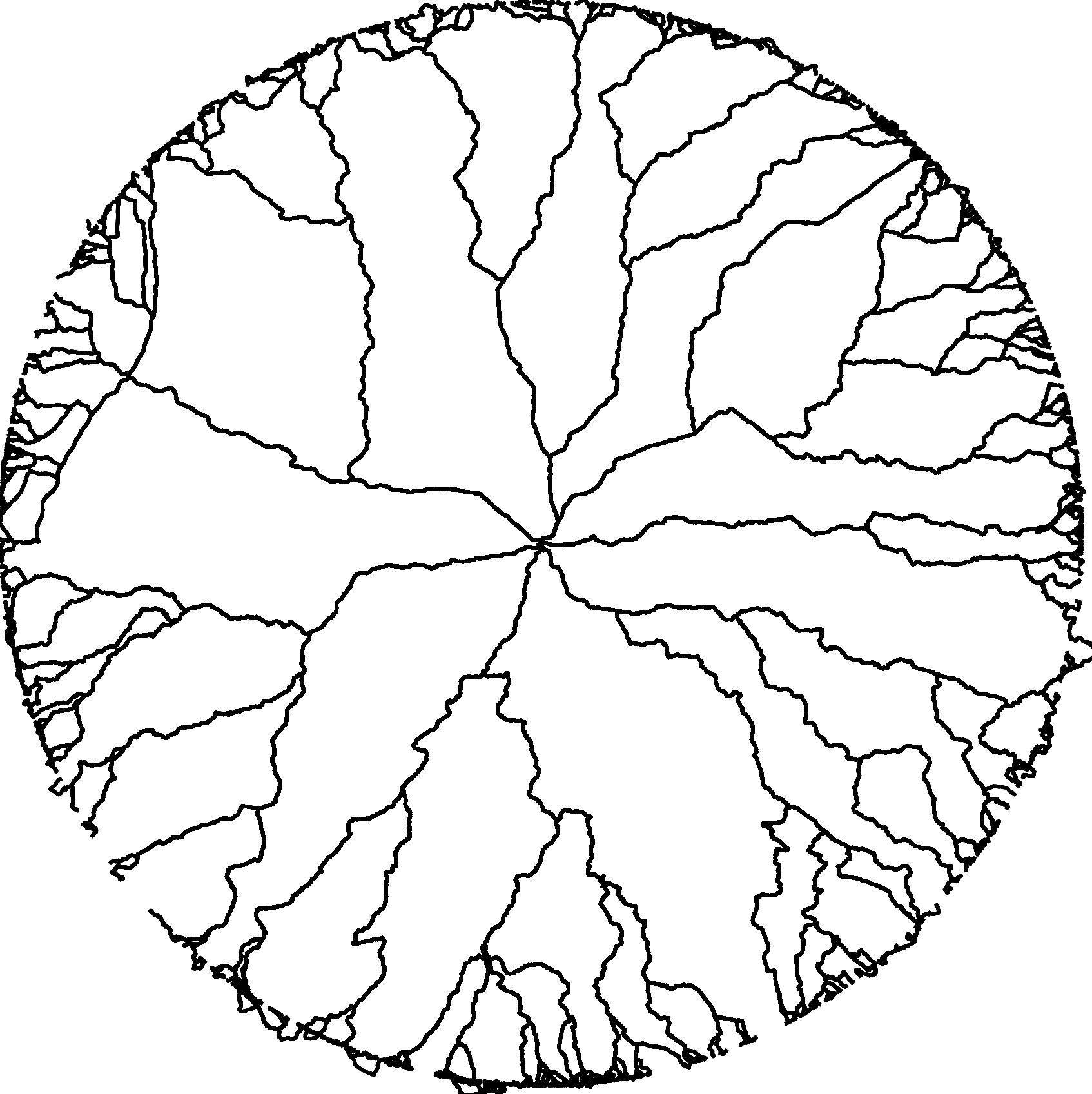
Figure 2: Shortest (left) and fastest (right) paths from a central point (near Munich, Germany) to $10^{4}$ randomly chosen points at a distance of $300$ km. The red arrow points to the most prominent overhang in the paths.

Let us first introduce more precisely the 2-dimensional DPRM problem and summarize the relevant results: A directed polymer is a chain pinned at its ends, and sufficiently stretched to prevent overhangs. Its wanderings can thus be described by a function $h(x)$, where $x$ is a coordinate along the axis between the end points and $h$ the distance from this axis. The cost (energy) of a configuration of is then given by

$$E[h(x)]=\int_{0}^{d}dx\left[\frac{\gamma}{2}\left(\frac{dh}{dx}\right)^{2}+V(x,h)\right]~{},$$ (1)

where $d$ is the Euclidean distance between the end points, $\gamma$ is the line tension of the chain and $V$ is a potential modeling a disordered environment. The canonical free energy at a temperature $T$ satisfies the KPZ equation KPZ that describes its scale invariant properties foot1 . In the zero-temperature limit, relevant to our problem, the free energy is simply the energy of the optimal path $E[h^{*}]$. Two exponents govern the scalings of the energy fluctuations $\left\langle(E-\langle E\rangle)^{2}\right\rangle\sim d^{2\beta}$ (where the brackets denote an average over realizations of the disorder $V$), and the transverse wanderings of the optimal chains, $\langle h^{*}(x)^{2}\rangle\sim x^{2\zeta}$ Kardar87 . In the simplest case of uncorrelated random potentials, the exponents are related by the identify $\beta=2\zeta-1$, and (in 2-dimensions) given by $\beta=1/3$ and $\zeta=2/3$ FNS77 . More recently, it has been shown that the full distribution of $E$ is universal, converging at large $d$ to the Tracy-Widom (TW) distributions of random matrix theory Prahofer00 ; Takeuchi11 ; THH15 . The KPZ exponent identity can break down for correlated potentials Medina89 ; long-range correlations in $V$ lead to larger scaling exponents and different energy distributions Peng91 ; Schorr03 ; Kloss14 ; Chu16 .

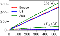
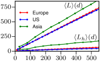
Figure 3: Average length of the optimal paths $\langle L\rangle$ and length of overhangs $\langle L_{h}\rangle$ as a function of the distance $d$ between the end points. All lengths are measured in km. Left: Shortest paths. Right: Fastest paths; $10^{6}$ points for each curve. Lines are guides to the eye.

In light of these theoretical results, we now analyze the statistics of two types of optimal paths (the shortest and the fastest) on the road network. We compute the paths using the Open Source Routing Machine (OSRM) OSRM operating on OpenStreetMap data, a collaborative effort to provide an open-source map of the world. The fastest paths are determined using the default configuration of OSRM which takes into account speed limitations for cars and road types, but no information on traffic. We gather six data sets for the two types of optimal paths in the three regions indicated in Fig. 1, sampling the end points of the paths uniformly on the network.

Figure 2 shows optimal paths from an arbitrary central point (near Munich, Germany) to uniformly sampled points at a distance of $300$ km. Both sets of optimal paths display fractal branching patterns resembling those of DPRM Kardar87 . However, these routes are not perfectly directed. This is especially visible near the end points where the local structure of the road network may impose overhangs (the most prominent is indicated by a red arrow in Fig. 2). Nevertheless, overhangs make a negligible contribution to the overall optimal trajectory. This is quantified in Fig. 3 where we plot the average length of the paths $\langle L\rangle(d)$ and the part $\langle L_{h}\rangle(d)$ corresponding to overhangs (see the Supplementary Information for a precise definition). The former increases linearly with separation $d$, while the latter grows sublinearly. Overhangs thus become less relevant at larger distances where we may expect a better correspondence between road paths and DPRM. In the following, we divide our study between short paths that are strongly constrained by local connectivity, and longer optimal paths that are directed.

Figure 4: Optimal paths between points at a distance $d=1$ km. Top: Probability distribution of the length $L$ of the shortest paths. Bottom: Probability distribution of the travel time $T$ of the fastest paths; $N=5\times 10^{5}$ paths for each curve.

We first look in Fig. 4 at the distribution of the length $L$ of the shortest paths (or the travel time $T$ on the fastest paths) between points at a small separation $d=1$ km. The distributions display clear power-law tails at large $L$ and $T$ over more than three orders of magnitude. The tails correspond to cases where the connecting path has to go around an obstacle to reach a nearby point, e.g. the next bridge across a river. They thus characterize the overhangs described previously. Most remarkably, the decay exponent $P(L)\sim L^{-\alpha}$ (and $P(T)\sim T^{-\alpha}$) seems to be universal across continents with $\alpha\approx 3$ (the best fit coefficients for the six curves are all within the range $[2.89;3.10]$). This is surprising since we expect paths at small $d$ to reflect the local structure of the road network which is a priori very different in the three regions considered. While we lack an explanation for the value of the exponent, we note its similarity to other problems in statistical physics: For self-avoiding random walks, the probability of loop lengths within a long chain is governed by $\alpha=2.68$ Duplantier87 ; Metzler02 while the shortest path between nearby points on the backbone of a percolation cluster also has $\alpha\approx 3$ Porto98 at small distances.

Due to the fat tails in the distributions of Fig. 4, the variances $\langle L^{2}\rangle_{c}(d)$ and $\langle T^{2}\rangle_{c}(d)$ are not defined, and cannot be used to estimate an exponent $\beta$ for cost fluctuations. Instead, we examine the full probability distributions $P(L|d)$ and $P(T|d)$ for increasing distance $d$, and attempt to make a “collapse” by superposing their maxima, and rescaling differences from the maximum by a factor $d^{\beta}$ chosen to best converge the distributions at large $d$. The results are shown in Fig. 5 (top) for the shortest paths in Europe, and in the Supplementary Information for the five other data sets, which show similar behavior. We find that the exponent $\beta$ can be adjusted such that the left tail of the distribution converges rapidly to a limit distribution well-fitted by the Tracy-Widom (TW) distribution expected for DPRM. By contrast, the right tail converges slowly and remains heavy at the largest $d$ attainable (larger $d$, comparable to the total size of the region, show strong finite-size effects). It is thus not clear if the right tail also converges to TW behavior or to a different distribution, as observed numerically for DPRM on a long-ranged correlated landscape Chu16 .

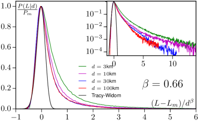
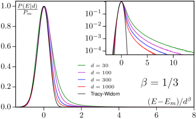
Figure 5: Top: Probability distribution of the length $L$ of the shortest paths in Europe rescaled with $\beta=0.66$; $5\times 10^{5}$ paths for each curve. Bottom: Probability distribution of the energy for a DPRM model (periodic boundary conditions on lattice of transverse size $10^{7}$) with power-law noise rescaled with $\beta=1/3$; $10^{7}$ paths for each curve. The insets show the same data with a logarithmic $y$-axis. $P_{m}$ denotes the maximum of the distribution, found at $L=L_{m}$ or $E=E_{m}$.

For comparison, we simulated a well-established DPRM model on a square lattice with paths directed along the diagonal Kardar87 ; Kim91 . The distance from the diagonal (parametrized by $x$) is again denoted by $h$. The energy of the optimal path is computed recursively as

$$E(x,h)=\text{min}\left\{E(x-1,h),E(x-1,h-1)\right\}+\eta(x,h).$$ (2)

After $d$ iterations, $E(d,h)$ is then the energy of the optimal path between the point $(d,h)$ and the line $d=0$. To mimic the short-scale distributions in Fig. 4, we draw the noise $\eta(d,h)$ from a power-law distribution $P(\eta)=2\eta^{-3}$ with $\eta\in[1;\infty[$. We then analyze the results as in the case of roads by shifting the energy distributions $P(E|d)$ to superimpose their maxima and rescaling their width by $d^{\beta}$ (Fig. 5, bottom). We observe that, as with Gaussian noise Kim91 , the distribution converges to a TW distribution with the KPZ exponent $\beta=1/3$. Indeed, only a fat tail in the noise at negative energy, $P(\eta)\sim\eta^{-a}$ as $\eta\to-\infty$ is expected to change the scaling exponents Pang93 ; Gueudre15 . Interestingly, the convergence upon increasing $d$ is similar in the model and the road data, with the right tails converging much slower. This also lends credence to our measure of $\beta$ as the exponent rescaling the left tail of the distributions.

The salient distinction between the paths on the road and DPRM is the value of the exponent $\beta$: The measured $\beta$ exponents are in the range $0.58$ and $0.9$ (with an estimated error of $15$%) are much larger than $\beta=1/3$ in the (uncorrelated) KPZ universality class. We argue that this can be explained by the presence of long-range correlations in the road network. To show this, we first discretize the full map of each region in squares of size $100\text{m}\times 100\text{m}$ and assign the value $\rho({\bf r})=1$ if a road is found inside the square and $0$ otherwise. We then compute the correlation function $C(r)=\langle\rho({\bf r})\rho({\bf r}+{\bf x})\rangle-\langle\rho({\bf x})\rangle^{2}$ where the average is taken over ${\bf x}$ and orientations of ${\bf r}$. As shown in Fig. 6, $C(r)$ decreases slowly (slower than $C(r)\sim r^{-0.5}$), remaining non-negligible on the scale of hundreds of kilometers. These long-range correlations reflect the shaping of the road network by factors acting at every scale, from different administrative divisions to natural obstacles. They were also shown to be important in modeling the development of cities Makse98 ; Barthelemy08 .

For DPRM, a power-law decay of correlations is known to be relevant from both numerical simulations Schorr03 ; Katsav04 ; Chu16 and renormalization group analysis Medina89 ; Katsav04 ; Kloss14 . For Gaussian noise with isotropic correlations decaying as a power-law with exponents between $-0.5$ and $-0.2$ (as measured for the road density correlations in Fig. 6), $\beta$ was measured between $0.5$ and $0.7$ Schorr03 . Given numerical and systematic uncertainties, these values are in relatively good agreement with our measurements for the road network. Long-range correlations are thus likely to be the cause of the observed large exponents.

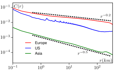
Figure 6: Auto-correlation functions of the road density as defined in the text. The oscillations in the curve for the US are not an artifact. The peaks are located every mile (with sub-peaks at half-miles) and correspond to large regions (up to 60 miles) of grid-like road network.

Finally, we look at the wanderings of the optimal paths in the transverse direction. The routing algorithm returns a list of points along each path (on average every $50$m) that we use to construct the function $h(x)$.We do so by discretizing the distance $x$ along the end-to-end axis in bins of size $dx=100$m, and averaging points falling in the same bin. This discards any overhangs and produces a directed path approximating the real path. For DPRM, transverse fluctuations scale as $\Delta h(x)=\sqrt{\langle h^{2}(x)\rangle}\sim x^{\zeta}$, but because of overhangs near the end points of road-paths $h(0)=\Delta h(0)\neq 0$ introducing large corrections to the putative scaling. Thus, as a first approximation, we estimate the exponent $\zeta$ by fitting $\Delta h(x)=a+bx^{\zeta}$ with free parameters $a$, $b$ and $\zeta$. The resulting functions $\Delta h(x)-a$ show scaling behavior over two orders of magnitude with exponents $\zeta\in[0.69;0.72]$ (see Fig. 7). Once again these values are larger than the uncorrelated KPZ value $\zeta=2/3$, but in qualitative agreement with the expected increase due to the presence of long-range correlations. For comparison, isotropic long-range correlations with decay exponent in the range of Fig. 6 give $\zeta\in[0.75;0.85]$ Schorr03 while correlations only in the transverse direction yield $\zeta\in[0.67;0.72]$ Chu16 .

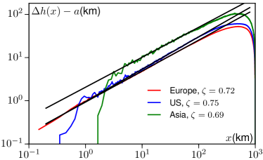
Figure 7: Transverse wanderings for the shortest paths as a function of the coordinate $x$ on the axis between the end points. Averages are over $5\times 10^{5}$ paths between points at distance $d=1000$ km.

To conclude, we have shown that optimal paths on the road network can be modeled as directed polymers in a random medium. To do so, we replaced the complex road structure by a random cost landscape featuring only the relevant properties needed to account for the observed statistics of optimal paths. We find two important such characteristics: At short scales, local connectivities result in circuitous paths with a scale-free distribution of lengths characterized by a universal power-law decay, a remarkable experimental fact that remains to be explained. This is mimicked by a power-law distributed noise in our DPRM model. At larger scales, the local structure becomes less relevant. The scaling of the path length/travel time and the transverse meanderings of optimal paths are then governed by long-range correlations that we show to be present in the network. Although these long-range correlations are non-universal, they show similar behaviors in the different regions of the world considered in this paper, leading to similar distributions at large scales. Directed polymers and associated theoretical results thus provide useful tools to understand the statistics of optimal paths on a complex network. It would be interesting in the future to see if this approach can be extended to other transportation networks or different environments, for example to the study of shortest paths on critical percolation clusters Barma86 , a problem with important practical applications.

- (1) D. J. Watts and S. H. Strogatz, Nature 393, 440 (1998).
- (2) A.-L. Barabàsi and R. Albert, Science 286, 509 (1999).
- (3) R. Albert and A.-L. Barabàsi, Reviews of Modern Physics 74, 47 (2002).
- (4) E. Ravasz and A.-L. Barabàsi, Physical Review E 67, 26112 (2003).
- (5) M. E. Newman, SIAM Review 45, 167 (2003).
- (6) J. Werfel, D.E. Ingber, and Y. Bar-Yam, Phys. Rev. Lett. 114, 238103 (2015).
- (7) A.J. Morales, V. Vavilala, R.M. Benito Benito, and Y. Bar-Yam, J. Royal Society Interface 14, 20161048 (2017).
- (8) M. Barthélemy, Physics Reports 499, 1 (2011).
- (9) M. Barthélemy and A. Flammini, Physical Review Letters 100, 138702 (2008).
- (10) A. Cardillo, S. Scellato, V. Latora, and S. Porta, Physical Review E 73, 066107 (2006).
- (11) S. Lämmer, B. Gehlsen, and D. Helbing, Physica A: Statistical Mechanics and Its Applications 363, 89 (2006).
- (12) P. S. Dodds and D. H. Rothman, Physical Review E 63, 16115 (2000).
- (13) P. Sen, S. Dasgupta, A. Chatterjee, P. Sreeram, G. Mukherjee, and S. Manna, Physical Review E 67, 036106 (2003).
- (14) D. Hunt and V. M. Savage, Physical Review E 93, 062305 (2016).
- (15) R. Geisberger, P. Sanders, D. Schultes, and D. Delling, in (Springer, 2008), pp. 319–333.
- (16) M. Kardar and Y.-C. Zhang, Physical Review Letters 58, 2087 (1987).
- (17) T. Halpin-Healy and Y.-C. Zhang, Physics Reports 254, 215 (1995).
- (18) M. Kardar, G. Parisi, and Y.-C. Zhang, Physical Review Letters 56, 889 (1986).
- (19) Because of this mapping, is traditionally denoted as a time direction but we stick here to the spacial notation to avoid confusion with travel times.
- (20) D. Forster, D.R. Nelson, and M.J. Stephen, Phys. Rev. A 16, 732 (1977).
- (21) M. Prähofer and H. Spohn, Physical Review Letters 84, 4882 (2000).
- (22) K. A. Takeuchi, M. Sano, T. Sasamoto, and H. Spohn, Nature Scientific Reports 1 34 (2011).
- (23) T. Halpin-Healy and K. A. Takeuchi, J. Stat. Phys. 160, 794 (2015).
- (24) E. Medina, T. Hwa, M. Kardar, and Y.-C. Zhang, Physical Review A 39, 3053 (1989).
- (25) C.-K. Peng, S. Havlin, M. Schwartz, and H. E. Stanley, Physical Review A 44, R2239 (1991).
- (26) T. Kloss, L. Canet, B. Delamotte, and N. Wschebor, Physical Review E 89, 22108 (2014).
- (27) S. Chu and M. Kardar, Physical Review E 94, 10101 (2016).
- (28) D. Luxen and C. Vetter, in Proceedings of the 19th ACM SIGSPATIAL International Conference on Advances in Geographic Information Systems (ACM, New York, NY, USA, 2011), pp. 513–516.
- (29) B. Duplantier, Physical Review B 35, 5290 (1987).
- (30) R. Metzler, A. Hanke, P.G. Dommersnes, Y. Kantor, and M. Kardar, Phys. Rev. Lett. 88, 188101 (2002).
- (31) M. Porto, S. Havlin, H. E. Roman, and A. Bunde, Physical Review E 58, R5205 (1998).
- (32) J. Kim, M. Moore, and A. Bray, Physical Review A 44, 2345 (1991).
- (33) T. Gueudre, P. Le Doussal, J.-P. Bouchaud, and A. Rosso, Physical Review E 91, 62110 (2015).
- (34) N.-N. Pang and T. Halpin-Healy, Physical Review E 47, R784 (1993).
- (35) R. Schorr and H. Rieger, The European Physical Journal B-Condensed Matter and Complex Systems 33, 347 (2003).
- (36) H. A. Makse, J. S. Andrade, M. Batty, S. Havlin, and H. E. Stanley, Physical Review E 58, 7054 (1998).
- (37) M. Barma and P. Ray, Physical Review B 34, 3403 (1986).
- (38) E. Katzav and M. Schwartz, Physical Review E 70, 011601 (2004).
- (39) T. Song and H. Xia, Journal of Statistical Mechanics: Theory and Experiment 2016, 113206 (2016).