Randomized Constraints Consensus for Distributed Robust Linear Programming

Abstract

In this paper we consider a network of processors aiming at cooperatively solving linear programming problems subject to uncertainty. Each node only knows a common cost function and its local uncertain constraint set. We propose a randomized, distributed algorithm working under time-varying, asynchronous and directed communication topology. The algorithm is based on a local computation and communication paradigm. At each communication round, nodes perform two updates: (i) a verification in which they check—in a randomized setup—the robust feasibility (and hence optimality) of the candidate optimal point, and (ii) an optimization step in which they exchange their candidate bases (minimal sets of active constraints) with neighbors and locally solve an optimization problem whose constraint set includes: a sampled constraint violating the candidate optimal point (if it exists), agent’s current basis and the collection of neighbor’s basis. As main result, we show that if a processor successfully performs the verification step for a sufficient number of communication rounds, it can stop the algorithm since a consensus has been reached. The common solution is—with high confidence—feasible (and hence optimal) for the entire set of uncertainty except a subset having arbitrary small probability measure. We show the effectiveness of the proposed distributed algorithm on a multi-core platform in which the nodes communicate asynchronously.

1 Introduction

Robust optimization plays an important role in several areas such as estimation and control and has been widely investigated. Its rich literature dates back to the $1950$s, see Ben-Tal and Nemirovski (2009) and references therein. Very recently, there has been a renewed interest in this topic in a parallel and/or distributed framework. In Lee and Nedić (2013), a synchronous distributed random projection algorithm with almost sure convergence is proposed for the case where each node has independent cost function and (uncertain) constraint. Since the distributed algorithm relies on extracting random samples from an uncertain constraint set, several assumptions on random set, network structure and agent weights are made to prove almost sure convergence. The synchronization of update rule relies on a central clock to coordinate the step size selection. To circumvent this limitation the same authors in Lee and Nedić (2016) present an asynchronous random projection algorithm in which a gossip-based protocol is used to desynchronize the step size selection. The proposed algorithms in (Lee and Nedić, 2013, 2016), require computing projection onto the constraint set at each iteration which is computationally demanding if the constraint set does not have a simple structure such as half space or polyhedron. In Carlone et al. (2014), a parallel/distributed scheme is considered for solving an uncertain optimization problem by means of the scenario approach (Calafiore and Campi, 2004). The scheme consists of extracting a number of samples from the uncertain set and assigning them to nodes in a network. Each node is assigned a portion of the extracted samples. Then, a variant of the constraints consensus algorithm introduced in Notarstefano and Bullo (2011) is used to solve the deterministic optimization problem. A similar parallel framework for solving convex optimization problems with one uncertain constraint via the scenario approach is considered in You and Tempo (2016). In this setup, the sampled optimization problem is solved in a distributed way by using a primal-dual subgradient (resp. random projection) algorithm over an undirected (resp. directed) graph. We remark that in Carlone et al. (2014); You and Tempo (2016), constraints and cost function of all agents are identical. In Bürger et al. (2014), a cutting plane consensus algorithm is introduced for solving convex optimization problem where constraints are distributed to the network processors and all processors have common cost function. In the case where constraints are uncertain, a worst-case approach based on a pessimizing oracle is used. The oracle relies on the assumption that constraints are concave with respect to uncertainty vector and the uncertainty set is convex. A distributed scheme based on the scenario approach is introduced in Margellos et al. (2016) in which random samples are extracted by each node from its local uncertain constraint set and a distributed proximal minimization algorithm is designed to solve the sampled optimization problem. The number of samples required to guarantee robustness can be large if the probabilistic levels defining robustness of the solution—accuracy and confidence levels—are stringent, possibly leading to a computationally demanding sampled optimization problem at each node.

The main contribution of this paper is the design of a fully distributed algorithm to solve an uncertain linear program in a network with directed and asynchronous communication. The problem under investigation is a linear program in which the constraint set is the intersection of local uncertain constraints, each one known only by a single node. Starting from a deterministic constraint exchange idea introduced in Notarstefano and Bullo (2011), the algorithm proposed in this paper introduces a randomized, sequential approach in which each node: (i) locally performs a probabilistic verification step (based on a local sampling of its uncertain constraint set), and (ii) solves a local, deterministic optimization problem with a limited number of constraints. If suitable termination conditions are satisfied, we are able to prove that the nodes agree on a common solution which is probabilistically feasible and optimal with high confidence. As compared to the literature above, the proposed algorithm has three main advantages. First, no assumptions are needed on the probabilistic nature of the local constraint sets. Second, each node can sample locally its own uncertain set. Thus, no central unit is needed to extract samples and no common constraint set needs to be known by the nodes. Third and final, nodes do not need to perform the whole sampling at the beginning and subsequently solve the (deterministic) optimization problem. Online extracted samples are used only for verification, which is computationally inexpensive. The optimization is performed always on a number of constraints that remains constant at each node and depends only on the dimension of the decision variable and on the number of node neighbors.

The paper is organized as follows. In Section 2, we formulate the uncertain distributed linear program (LP). Section 3 presents our distributed sequential randomized algorithm for finding a solution—with probabilistic robustness—to the uncertain distributed LP. The probabilistic convergence properties of the distributed algorithm are investigated in Section 4. Finally, extensive numerical simulations are performed in Section 5 to prove the effectiveness of the proposed methodology.

2 Problem Formulation

We consider a network of processors with limited computation and/or communication capabilities that aim at cooperatively solving the following uncertain linear program

$$\underset{\theta}{\min} ~{}~{}c^{T}\theta$$

subject to $$~{}~{}A_{i}^{T}(q)\theta\leq b_{i}(q),\;\forall q\in\mathbb{Q},~{}i\in\{1,\ldots,n\},$$ (1)

where $\theta\in\Theta\subset\mathbb{R}^{d}$ is the vector of decision variables, $q\in\mathbb{Q}$ is the uncertainty vector, $c\in\mathbb{R}^{d}$ defines the objective direction, $A_{i}(q)\in\mathbb{R}^{m_{i}\times d}$ and $b_{i}(q)\in\mathbb{R}^{m_{i}}$, with $m_{i}\geq d$, define the (uncertain) constraint set of agent $i\in\{1,\ldots,n\}$. Processor $i$ has only knowledge of a constraint set defined by $A_{i}(q)$ and $b_{i}(q)$ and the objective direction $c$ (which is the same for all nodes). Each node runs a local algorithm and by exchanging limited information with neighbors, all nodes converge to the same solution. We want to stress that there is no (central) node having access to all constraints. We make the following assumption regarding problem (1).

Assumption 1 (Non-degeneracy)

The minimum point of any subproblem of (1) with at least $d$ constraints is unique and there exist only $d$ constraints intersecting at the minimum point.

We let the nodes communicate according to a time-dependent, directed communication graph $\mathcal{G}(t)=\{\mathcal{V},\mathcal{E}(t)\}$ where $t\in{\mathbb{N}}$ is a universal time, $\mathcal{V}=\{1,\ldots,n\}$ is the set of agent identifiers and $(i,j)\in\mathcal{E}(t)$ indicates that $i$ send information to $j$ at time $t$. The time-varying set of incoming (resp. outgoing) neighbors of node $i$ at time $t$, $\mathcal{N}_{\text{in}}(i,t)$ ($\mathcal{N}_{\text{out}}(i,t)$), is defined as the set of nodes from (resp. to) which agent $i$ receives (resp. transmits) information at time $t$. A directed static graph is said to be strongly connected if there exists a directed path (of consecutive edges) between any pair of nodes in the graph. For time-varying graphs we use the notion of uniform joint strong connectivity formally defined next.

Assumption 2 (Uniform joint strong connectivity)

There exists an integer $L\geq 1$ such that the graph $\bigg{(}\mathcal{V},\bigcup_{\tau=t}^{t+L-1}\mathcal{E}(\tau)\bigg{)}$ is strongly connected for all $t\geq 0$.

There is no assumption on how uncertainty $q$ enters problem (1) making it computationally difficult to solve. In fact, if the uncertainty set $\mathbb{Q}$ is an uncountable set, problem (1) is a semi-infinite optimization problem involving infinite number of constraints. In general, there are two main paradigms to solve an uncertain optimization problem of form (1). The first approach is a deterministic worst-case paradigm in which the constraints are enforced to hold for all possible uncertain parameters in the set $\mathbb{Q}$. This approach is computationally intractable for cases where uncertainty does not appear in a “simple” form, e.g. affine, multi-affine, convex, etc. The second approach is a probabilistic approach where uncertain parameters are considered to be random variables and the constraints are enforced to hold for the entire set of uncertainty except a subset having an arbitrary small probability measure. In this paper, we follow a probabilistic approach and present a distributed tractable randomized setup for finding a solution—with desired probabilistic properties—for the optimization problem (1).

Notation
The constraint set of agent $i$ is defined by

$$H^{i}(q)\doteq[A_{i}(q),b_{i}(q)].$$

Throughout this paper, we use capital italic letter, e.g. $H^{i}(q)\doteq[A_{i}(q),b_{i}(q)]$ to denote a collection of half spaces and capital calligraphic letter, $\mathcal{H}^{i}(q)$ to denote the set induced by half spaces, i.e. $\mathcal{H}^{i}(q)\doteq\{\theta\in\mathbb{R}^{d}:A_{i}(q)\leq b_{i}(q)\}$. We note that, with this notation, if $A=B\cup C$ with $B$ and $C$ being collection of half spaces, then $\mathcal{A}=\mathcal{B}\cap\mathcal{C}$, that is, the set induced by the union of constraint sets $B$ and $C$ is the intersection of $\mathcal{B}$ and $\mathcal{C}$. Finally $J(H)$ is the smallest value of $c^{T}\theta$ while $\theta\in\mathcal{H}$. The linear program specific to each agent $i\in\mathcal{V}$ is fully characterized by the pair $(H^{i}(q),c)$ (note that $c$ defines the objective direction which is the same for all nodes).

3 Randomized Constraints Consensus

In this section, we present a distributed, randomized algorithm for solving the uncertain linear program (LP) (1) in a probabilistic sense. First, recall that the solution of a linear program of the form (1) can be identified by at most $d$ active constraints ($d$ being the dimension of the decision variable). This concept is formally characterized by the notion of basis. Given a collection of constraints $H$, a subset $B\subseteq H$ is a basis of $H$ if the optimal cost of the LP problem defined by $(H,c)$ is identical to the one defined by $(B,c)$, and the optimal cost decreases if any constraint is removed from $B$. We define a primitive $[\theta^{*},B]={\texttt{Solve\textsubscript{LP}}}(H,c)$ which solves the LP problem defined by the pair $(H,c)$ and returns back the optimal point $\theta^{*}$ and the corresponding basis $B$.

Note that, since the uncertainty set is uncountable, it is in general very difficult to verify if a candidate solution is feasible for the entire set of uncertainty or not. We instead use a randomized approach based, on Monte Carlo simulation, to check probabilistic feasibility. The distributed algorithm we propose has a probabilistic nature consisting of two main steps: verification and optimization. The main idea is the following. A node has a candidate basis and candidate solution point. First, it verifies if the candidate solution point belongs to its local uncertain set with high probability. Then, it collects bases from neighbors and solves an LP with its basis and its neighbors’ bases as constraint set. If the verification step was not successful, the first violating constraint is also added to the problem.

Formally, we assume that $q$ is a random variable and a probability measure ${\mathbb{P}}$ over the Borel $\sigma-$algebra of $\mathbb{Q}$ is given. In the verification step each agent $i$ generates $M_{k_{i}}$ independent and identically distributed (i.i.d) random samples from the set of uncertainty

$${{\rm\bf q}}_{k_{i}}\doteq\{q^{(1)},\ldots,q^{(M_{k_{i}})}\}\in\mathbb{Q}^{M_{k_{i}}},$$

according to the measure ${\mathbb{P}}$, where ${k_{i}}$ is a local counter keeping track of the number of times the verification step is performed and $\mathbb{Q}^{M_{k_{i}}}\doteq\mathbb{Q}\times\ldots\times\mathbb{Q}$ ($M_{k_{i}}$ times). Using a Monte Carlo algorithm, node $i$ checks feasibility of the candidate solution $\theta^{i}(t)$ only at the extracted samples. If a violation happens, the first violating sample is used as a violation certificate. In the optimization step, agent $i$ transmits its current basis to all outgoing neighbors and receives bases from incoming ones. Then, it solves an LP problem whose constraint set is composed of: i) a constraint constructed at the violation certificate (if it exists) ii) its current basis and iii) the collection of bases from all incoming neighbors. Node $i$ repeats these two steps until a termination condition is satisfied, namely if the candidate basis has not changed for $2nL+1$ times, with $L$ defined in Assumption 2. The distributed algorithm is formally presented in Algorithm 1.

Algorithm 1 Randomized Constraints Consensus

Input: $(H^{i}(q),c),\varepsilon_{i},\delta_{i}$

Output: $\theta_{\text{sol}}$

Initialization:
Set $k_{i}=1,[\theta^{i}(1),B^{i}(1)]={\texttt{Solve\textsubscript{LP}}}(H^{i}(\mathbf{0}),c)$

Evolution:

1. Verification:

   • If $\theta^{i}(t)=\theta^{i}(t-1)$, set $q_{\texttt{viol}}=\emptyset$ and goto (ii)

   • Extract

     $$M_{k_{i}}\geq\frac{2.3+1.1\ln k_{i}+\ln\frac{1}{\delta_{i}}}{\ln\frac{1}{1-\varepsilon_{i}}}$$ (2)

     i.i.d samples ${{\rm\bf q}}_{k_{i}}=\{q_{k_{i}}^{(1)},\ldots,q_{k_{i}}^{(M_{k_{i}})}\}$

   • If $\theta^{i}(t)\in\mathcal{H}^{i}(q_{k_{i}}^{(\ell)})$ for all $\ell=1,\ldots,M_{k_{i}}$, set $q_{\texttt{viol}}=\emptyset$; else, set $q_{\texttt{viol}}$ as the first sample for which $\theta^{i}(t)\notin\mathcal{H}^{i}(q_{\texttt{viol}})$

   • Set $k_{i}=k_{i}+1$

2. Optimization:

   • Transmit $B^{i}(t)$ to $j\in\mathcal{N}_{\text{out}}(i,t)$ and acquire incoming neighbors basis $Y^{i}(t)\doteq\cup_{j\in\mathcal{N}_{\text{in}}(i,t)}B^{j}$

   • $[\theta^{i}(t+1),B^{i}(t+1)]=$
     $~{}~{}~{}~{}~{}~{}~{}~{}~{}~{}~{}~{}~{}{\texttt{Solve\textsubscript{LP}}}(H^{i}(q_{\texttt{viol}})\cup B^{i}(t)\cup Y^{i}(t),c)$

   • If $\theta^{i}(t+1)$ has not changed for $2nL+1$ times and $q_{\texttt{viol}}=\emptyset$, return $\theta_{\text{sol}}=\theta^{i}(t+1)$

The counter $k_{i}$ counts the number of times the verification step is called. We remark that if at some $t$ the candidate solution has not changed, that is $\theta^{i}(t)=\theta^{i}(t-1)$, then $\theta^{i}(t-1)$ has successfully satisfied the verification step and $q_{\texttt{viol}}=\emptyset$ at time $t-1$ and therefore there is no need to check it again.

Remark 1 (Asynchronicity)

The distributed algorithm presented in this section is completely asynchronous. Indeed, time $t$ is just a universal time that does not need to be known by the nodes. The time-dependent jointly connected graph then captures the fact that nodes can perform computation at different speeds.

Remark 2

In the deterministic constraints consensus algorithm presented in Notarstefano and Bullo (2011), at each iteration of the algorithm, the original constraint set of the node needs to be taken into account in the local optimization problem. Here, we can drop this requirement because of the verification step.

4 Analysis of Randomized Constraints Consensus algorithm

In this section, we analyze the convergence properties of the distributed algorithm and investigate the probabilistic properties of the solution computed by the algorithm.

Theorem 1

Let Assumptions 1 and 2 hold. Given the probabilistic levels $\varepsilon_{i}>0$ and $\delta_{i}>0$, $i=1,\ldots,n$, let $\varepsilon=\sum_{i=1}^{n}\varepsilon_{i}$ and $\delta=\sum_{i=1}^{n}\delta_{i}$. Then, the following statements hold

1. Along the evolution of Algorithm 1, the cost $J(B^{i}(t))$ at each node $i\in\{1,\ldots,n\}$ is monotonically non-decreasing. That is, $J(B^{i}(t+1))\geq J(B^{i}(t))$.

2. The cost $J(B^{i}(t))$ for all $i\in\{1,\ldots,n\}$ converges to a common value asymptotically. That is, $\lim_{t\rightarrow\infty}J(B^{i}(t))=\bar{J}$ for all $i\in\{1,\ldots,n\}$.

3. If the candidate solution of node $i$, $\theta^{i}(t)$, has not changed for $2Ln+1$ communication rounds, all nodes have a common candidate solution $\theta_{\text{sol}}$.

4. The following inequality holds for $\theta_{\text{sol}}$

   $${\mathbb{P}}^{M}\bigg{\{} {{\rm\bf q}}\in\mathbb{Q}^{M}:$$

   $${\mathbb{P}}\bigg{\{}q\in\mathbb{Q}:\theta_{\text{sol}}\notin\bigcap_{i=1}^{n}\mathcal{H}^{i}(q)\bigg{\}}\leq\varepsilon\bigg{\}}\geq 1-\delta,$$

   where $M$ is the cardinality of the collection of multisamples of all agents.

5. Let $B_{\text{sol}}$ be the basis corresponding to $\theta_{\text{sol}}$. The following inequality holds for $B_{\text{sol}}$

   $${\mathbb{P}}^{M}\bigg{\{}{{\rm\bf q}}\in\mathbb{Q}^{M}:{\mathbb{P}}\bigg{\{}q\in\mathbb{Q}:J \big{(}B_{\text{sol}}\cup H(q)\big{)}>J(B_{\text{sol}})\bigg{\}}$$

   $$\leq\varepsilon\bigg{\}}\geq 1-\delta$$

   where $H(q)\doteq\bigcup_{i=1}^{n}H^{i}(q)$ and $M$ is the cardinality of the collection of multisamples of all agents.

Proof of first statement:
The set of constraints at time $t+1$ consists of the node current basis $B^{i}(t)$, the collection of neighbors’ bases $Y^{i}(t)\doteq\cup_{j\in\mathcal{N}_{\text{in}}(i,t)}B^{j}$ and $H^{i}(q_{\texttt{viol}})$. Since the basis at time $t$, $B^{i}(t)$, is part of the constraint set for computing $B^{i}(t+1)$, $J(B^{i}(t+1))$ cannot be smaller than $J(B^{i}(t))$.

Proof of second and third statements:
Since the graph is uniformly jointly strongly connected, for any pairs of nodes $u$ and $v$ and for any $t>0$, there exists a time-dependent path from $u$ to $v$ (Hendrickx, 2008)—a sequence of nodes $\ell_{1},\ldots,\ell_{k}$ and a sequence of time instances $t_{1},\ldots,t_{k+1}$ with $t\leq t_{1}<\ldots<t_{k+1}$, such that the directed edges $\{(u,\ell_{1}),(\ell_{1},\ell_{2}),\ldots,(\ell_{k},v)\}$ belongs to the directed graph at time instances $\{t_{1},\ldots,t_{k+1}\}$, respectively—of length at most $nL$. We recall that $n$ is the number of nodes and $L$ is defined in Assumption 2. Consider nodes $i$ and $p$. If $\ell_{1}\in\mathcal{N}_{\text{out}}(i,t_{0})$, then $J(B^{i}(t_{0}))\leq J(B^{\ell_{1}}(t_{0}+1))$ as the constraint set of node $\ell_{1}$ at time $t_{0}+1$ is a superset of the constraint set of node $i$ at time $t_{0}$. Iterating this argument, we obtain $J(B^{i}(t_{0}))\leq J(B^{p}(t_{0}+nL))$. Again since the graph is uniformly jointly strongly connected, there will be a time varying path of length at most $nL$ from node $p$ to node $i$. Therefore,

$$J(B^{i}(t_{0}))\leq J(B^{p}(t_{0}+nL))\leq J(B^{i}(t_{0}+2nL)).$$

Two scenarios can happen proving respectively statements (ii) and (iii).

If $J(B^{i}(t_{0}))\neq J(B^{i}(t_{0}+2nL))$, then $J(B^{i}(t_{0}))<J(B^{i}(t_{0}+2nL))$ which means the cost at node $i$ is strictly increasing. Denote by $J^{*}$ the optimal cost associated to problem (1). Since the problem at each node can be considered as a sub-problem of (1), the sequence $\{J(B^{i}(t))\}_{t>0}$ is convergent and has a limit point $\bar{J}^{i}\leq J^{*}$, i.e. $\lim_{t\rightarrow\infty}J(B^{i}(t))\rightarrow\bar{J}^{i}$ for all $i\in\mathcal{V}$. In what follows, we prove that the limit point of all agents are the same, that is $\bar{J}^{1}=\ldots=\bar{J}^{n}$. We follow a similar reasoning as in (Bürger et al., 2014, Lemma IV.2). Suppose by contradiction that there exist two processors $i$ and $p$ such that $\bar{J}^{i}>\bar{J}^{p}$. There exists $\eta_{0}>0$ such that $\bar{J}^{i}-\bar{J}^{p}>\eta_{0}$. Since the sequences $\{J(B^{i}(t))\}_{t>0}$ and $\{J(B^{p}(t))\}_{t>0}$ are monotonically increasing and convergent, for any $\eta>0$, there exists a time $T_{\eta}$ such that for all $t\geq T_{\eta}$, $\bar{J}^{i}-J(B^{i}(t))\leq\eta$ and $\bar{J}^{p}-J(B^{p}(t))\leq\eta$. This implies that there exists a $T_{\eta_{0}}$ such that for all $t\geq T_{\eta_{0}}$, $J(B^{i}(t))\geq\bar{J}^{i}-\eta_{0}>\bar{J}^{p}$. Additionally, since the objective function is increasing, it follows that for any time instant $t^{\prime}\geq 0$, $J(B^{p}(t^{\prime}))\leq\bar{J}^{p}$. Thus, for all $t\geq T_{\eta_{0}}$ and all $t^{\prime}\geq 0$

$$J(B^{i}(t))>J(B^{p}(t^{\prime})).$$ (3)

On the other hand, since the graph is uniformly jointly strongly connected, there exists a time-varying path of length at most $nL$ from node $i$ to node $p$. Therefore, for all $t\geq T_{\eta_{0}}$

$$J(B^{i}(t))\leq J(B^{p}(t+nL)).$$ (4)

However, (4) contradicts (3) proving that $J^{1}=\ldots=J^{n}$. Therefore, it must hold that $\lim_{t\rightarrow\infty}|J(B^{i}(t))-J(B^{j}(t))|\rightarrow 0$ for all $i,j\in\mathcal{V}$. This proves the second statement of the theorem.

If $J(B^{i}(t_{0}))=J(B^{i}(t_{0}+2nL))$ and considering the point that node $p$ can be any node of the graph, then all nodes have the same cost. That is, $J(B^{1}(t))=\ldots=J(B^{n}(t))$. This combined with Assumption 1 proves the third statement of the theorem. That is, if the candidate solution is not updated for $2nL+1$ communication rounds, all nodes have a common solution and hence the distributed algorithm can be halted.

Proof of forth statement:
We first note that using (Chamanbaz et al., 2016, Theorem 1), (Calafiore and Dabbene, 2007, Theorem 3) and (Dabbene et al., 2010, Theorem 5.3) we can show that—at any iteration $t$—if the sample size is selected based on (2) and the verification step is successful, that is $q_{\texttt{viol}}=\emptyset$, then

$${\mathbb{P}}^{M}\left\{{{\rm\bf q}}\in\mathbb{Q}^{M}:{\mathbb{P}}\{q\in\mathbb{Q}:\theta^{i}(t)\notin\mathcal{H}^{i}(q)\}\leq\varepsilon_{i}\right\}\geq 1-\delta_{i}.$$

We note that the above inequality is a centralized result and holds only for the agent’s own constraint $\mathcal{H}^{i}(q)$. Also since for $\theta_{\text{sol}}$, the verification has to be successful, then

$${\mathbb{P}}^{M}\left\{{{\rm\bf q}}\in\mathbb{Q}^{M}:{\mathbb{P}}\{q\in\mathbb{Q}:\theta_{\text{sol}}\notin\mathcal{H}^{i}(q)\}\leq\varepsilon_{i}\right\}\geq 1-\delta_{i}.$$ (5)

We further remark that the sample bound (2) is obtained by replacing $k_{t}-1$, $\delta/2$ and $\gamma$ in (Chamanbaz et al., 2016, Eq. (10)) with $\infty$, $\delta_{i}$ and $1.1$ respectively, see (Chamanbaz et al., 2016, Remark 1) for a discussion on optimal value of $\gamma$.

Now, we are interested in bounding the probability by which $\theta_{\text{sol}}\notin\bigcap_{i=1}^{n}\mathcal{H}^{i}(q)$, i.e.

$${\mathbb{P}}^{M}\left\{{{\rm\bf q}}\in\mathbb{Q}^{M}:{\mathbb{P}}\left\{q\in\mathbb{Q}:\theta_{\text{sol}}\notin\bigcap_{i=1}^{n}\mathcal{H}^{i}(q)\right\}\leq\varepsilon\right\}.$$ (6)

In order to bound (6), we follow similar reasoning stated in Margellos et al. (2016). Define the following events

$${\textrm{Bad}}_{i}\doteq\{\theta_{\text{sol}}\notin\mathcal{H}^{i}(q),\forall q\in\mathbb{Q}\}$$

$${\textrm{Bad}}\doteq\{\theta_{\text{sol}}\notin\bigcap_{i=1}^{n}\mathcal{H}^{i}(q),\forall q\in\mathbb{Q}\}.$$

Equations (5) and (6) can be written in terms of the events Bad_i and Bad

$${\mathbb{P}}^{M}\left\{{{\rm\bf q}}\in\mathbb{Q}^{M}:{\mathbb{P}}\{{\textrm{Bad}}_{i}\}\leq\varepsilon_{i}\right\}\geq 1-\delta_{i}$$ (7)

$${\mathbb{P}}^{M}\left\{{{\rm\bf q}}\in\mathbb{Q}^{M}:{\mathbb{P}}\{{\textrm{Bad}}\}\leq\varepsilon\right\}$$ (8)

respectively. One can observe that

$$\theta_{\text{sol}}\notin\bigcap_{i=1}^{n}\mathcal{H}^{i}(q)\Rightarrow\exists i\in\{1,\ldots,n\}:\theta_{\text{sol}}\notin\mathcal{H}^{i}(q).$$

Hence, the event Bad can be written as the union of events ${\textrm{Bad}}_{i},~{}i=1,\ldots,n$, that is ${\textrm{Bad}}={\textrm{Bad}}_{1}\cup{\textrm{Bad}}_{2}\cup\ldots\cup{\textrm{Bad}}_{n}$. Invoking Boole’s inequality (Comtet, 1974) (also known as Bonferroni’s inequality), we have

$${\mathbb{P}}\{{\textrm{Bad}}\}\leq\sum_{i=1}^{n}{\mathbb{P}}\{{\textrm{Bad}}_{i}\}.$$ (9)

Replacing ${\mathbb{P}}\{{\textrm{Bad}}\}$ in (8) with the right hand side of (9) we obtain

$${\mathbb{P}}^{M}\left\{{{\rm\bf q}}\in\mathbb{Q}^{M}:\sum_{i=1}^{n}{\mathbb{P}}\{{\textrm{Bad}}_{i}\}\leq\varepsilon\right\}$$

$$= {\mathbb{P}}^{M}\left\{{{\rm\bf q}}\in\mathbb{Q}^{M}:\sum_{i=1}^{n}{\mathbb{P}}\{{\textrm{Bad}}_{i}\}\leq\sum_{i=1}^{n}\varepsilon_{i}\right\}$$

$$\geq {\mathbb{P}}^{M}\left\{\bigcap_{i=1}^{n}\left\{{{\rm\bf q}}\in\mathbb{Q}^{M}:{\mathbb{P}}\{{\textrm{Bad}}_{i}\}\leq\varepsilon_{i}\right\}\right\}$$

$$\geq 1-\sum_{i=1}^{n}{\mathbb{P}}^{M}\left\{{{\rm\bf q}}\in\mathbb{Q}^{M}:{\mathbb{P}}\{{\textrm{Bad}}_{i}\}>\varepsilon_{i}\right\}$$

$$\geq 1-\sum_{i=1}^{n}\delta_{i}=1-\delta.$$

We remark that the third line of above equation comes from the fact that if ${\mathbb{P}}\{{\textrm{Bad}}_{i}\}\leq\varepsilon_{i},~{}\forall i=1,\ldots,n$ then, one can ensure that $\sum_{i=1}^{n}{\mathbb{P}}\{{\textrm{Bad}}_{i}\}\leq\sum_{i=1}^{n}\varepsilon_{i}$. The forth line also is due to the fact that ${\mathbb{P}}\{\bigcap_{i}A_{i}\}=1-{\mathbb{P}}\{\bigcup_{i}A_{i}^{c}\}$ where $A_{i}^{c}$ is the complement of the event $A_{i}$.

Proof of fifth statement:
We first note that if the solution $\theta_{\text{sol}}$ is violated for a sample $q_{v}$ from the set of uncertainty, that is, $\theta_{\text{sol}}\notin\bigcap_{i=1}^{n}\mathcal{H}^{i}(q_{v})$, then $J(B_{\text{sol}}\cup H(q_{v}))\geq J(B_{\text{sol}})$ with $H(q_{v})\doteq\bigcup_{i=1}^{n}H^{i}(q_{v})$. However, due to Assumption 1, any subproblem of (1) has a unique minimum point and hence, $J(B_{\text{sol}}\cup H(q_{v}))\neq J(B_{\text{sol}})$. This argument combined with the result of forth statement proves the fifth statement of the theorem. That is, the probability that the solution $\theta_{\text{sol}}$ is no longer optimal for a new sample equals the probability that the solution is violated by the new sample.

$\blacksquare$

5 Numerical Simulation

We test the effectiveness of the distributed algorithm presented in Section 3 through extensive numerical simulations. To this end, we generate random linear programs (LP)—with a large number of uncertain parameters—assigned to various nodes of the network. Each node is assigned an uncertain set of the form

$$(A^{0}+A_{q})^{T}\theta\leq b,$$

where $A^{0}$ is a fixed (nominal) matrix and $A_{q}$ is an interval matrix—a matrix whose entries are bounded in given intervals—defining the uncertainty in the optimization problem. We follow the methodology presented in Dunham et al. (1977) in order to generate $A^{0},~{}b$ and the problem cost $c$ such that the linear program is always feasible. In particular, elements of $A^{0}$ are drawn from standard Gaussian distribution (mean$=0$ and variance$=1$). The $i$-th element of $b$ is define by $b_{i}=(\sum_{j=1}^{d}A^{0}_{ij})^{1/2}$. The objective direction $c$—which is the same for all the nodes—is also drawn from the standard Gaussian distribution. The communication graph $\mathcal{G}$ is a random connected graph with fixed number of neighbors.

Table 1: The average—over all nodes—number of times a basis is transmitted to the neighbors, average number of times verification is performed ($k_{i}$ at the convergence) and empirical violation of the computed solution ($\theta_{\text{sol}}$) over $10,000$ random samples for different number of nodes and neighbors in each node. The simulation is performed $100$ times for each row and average results are reported.

# Nodes	# Neighbors	Graph	#Constraints	# Transmissions	$k_{i}$ at convergence	Empirical
$n$	in each node	diameter	in each node	(averaged)	(averaged)	violation
$10$	$3$	$4$	$100$	$29.57$	$31.69$	$2.81\times 10^{-4}$
$20$	$4$	$4$	$100$	$26.92$	$29.02$	$1.7\times 10^{-4}$
$50$	$6$	$4$	$100$	$26.47$	$28.51$	$7\times 10^{-5}$
$100$	$7$	$4$	$100$	$26.63$	$28.68$	$2.9\times 10^{-5}$

A workstation with $12$ cores and $48$ GB of RAM is used to emulate the network model. From an implementation viewpoint, each node executes Algorithm 1 in an independent Matlab environment and the communication is modeled by sharing files between different Matlab environments. We use the linprog function of Mosek (Andersen and Andersen, 2000) to solve optimization problems appearing at each iteration of the distributed algorithm.

In Table 1, we change the number of nodes and neighbors such that the graph diameter is always $4$. The number of constraints in each node is also kept at $100$. We set the dimension of decision variables to $d=5$ and consider all elements of $A_{q}$ to be bounded in $[-0.2,0.2]$. The underlying probability distribution is selected to be uniform due to its worst-case nature. The probabilistic accuracy and confidence levels of each agent ($\varepsilon_{i}$ and $\delta_{i}$) are $0.1/n$ and $10^{-8}/n$ respectively, with $n$ being the number of nodes (first column of Table 1). We report the average—over all nodes—number of times each node updates its basis and transmits it to the outgoing neighbors. It is assumed that each node keeps the latest information received from neighbors and hence, if the basis is not updated, there is no need to re-transmit it to the neighbors. This also accounts for the asynchronicity of the distributed algorithm. We also report the average—over all nodes—number of times node $i$ performs the verification step, i.e., $k_{i}$ at convergence. This allows us to show that with a small number of “design” samples used in the optimization step, nodes compute a solution with high degree of robustness. In order to examine robustness of the obtained solution, we run an aposteriori analysis based on Monte Carlo simulation. To this end, we collect all the constraints across different nodes in a single problem of form (1) and check—in a centralized setup—the feasibility of the obtained solution for $10,000$ random samples extracted from the uncertain set. The empirical violation (last column of Table 1) is measured by dividing the number of samples that violate the solution by $10,000$. Since Algorithm 1 has a stochastic nature, we run the simulation $100$ times for each row of Table 1 and report the average values.

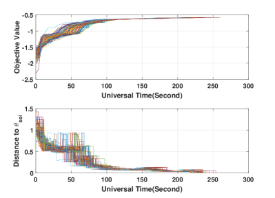
Figure 1: Objective value and distance to $\theta_{\text{sol}}$ for all the nodes in the network corresponding to the last row of Table 1.

We remark that it is very difficult in practice to check if Assumption 1 is satisfied for a given problem. However, we observe that in all the simulations reported here, the candidate solutions converge to the same point in finite time. In Figure 1, we report the objective value and the distance of candidate solutions $\theta^{i}(t),\forall i\in\{1,\ldots,n\}$ from $\theta_{\text{sol}}$ along the distributed algorithm execution for a problem instance corresponding to the last row of Table 1. It is observed that all the nodes converge to the same solution $\theta_{\text{sol}}$.

6 Conclusions

In this paper, we proposed a randomized distributed algorithm for solving robust linear programs (LP) in which the constraint sets are scattered across a network of processors communicating according to a directed time-varying graph. The distributed algorithm has a sequential nature consisting of two main steps: verification and optimization. Each processor iteratively verifies a candidate solution through a Monte Carlo algorithm, and solves a local LP whose constraint set includes its current basis, the collection of bases from neighbors and possibly, a constraint—provided by the Monte Carlo algorithm—violating the candidate solution. The two steps, i.e. verification and optimization, are repeated till a local stopping criteria is met and all nodes converge to a common solution. We analyze the convergence properties of the proposed algorithm.

References

- Andersen and Andersen (2000) Andersen, E. and Andersen, K. (2000). The mosek interior point optimizer for linear programming: an implementation of the homogeneous algorithm. In High performance optimization, 197–232. Springer.
- Ben-Tal and Nemirovski (2009) Ben-Tal, A.and El Ghaoui, L. and Nemirovski, A. (2009). Robust optimization. Princeton University Press.
- Bürger et al. (2014) Bürger, M., Notarstefano, G., and Allgöwer, F. (2014). A polyhedral approximation framework for convex and robust distributed optimization. IEEE Transactions on Automatic Control, 59, 384–395.
- Calafiore and Dabbene (2007) Calafiore, G. and Dabbene, F. (2007). A probabilistic analytic center cutting plane method for feasibility of uncertain lmis. Automatica, 43, 2022–2033.
- Calafiore and Campi (2004) Calafiore, G. and Campi, M. (2004). Uncertain convex programs: randomized solutions and confidence levels. Mathematical Programming, 102, 25–46.
- Carlone et al. (2014) Carlone, L., Srivastava, V., Bullo, F., and Calafiore, G. (2014). Distributed random convex programming via constraints consensus. SIAM Journal on Control and Optimization, 52, 629–662.
- Chamanbaz et al. (2016) Chamanbaz, M., Dabbene, F., Tempo, R., Venkataramanan, V., and Wang, Q.G. (2016). Sequential randomized algorithms for convex optimization in the presence of uncertainty. IEEE Transactions on Automatic Control, 61, 2565–2571.
- Comtet (1974) Comtet, L. (1974). Sieve Formulas, 176–203. Springer Netherlands, Dordrecht.
- Dabbene et al. (2010) Dabbene, F., Shcherbakov, P., and Polyak, B. (2010). A randomized cutting plane method with probabilistic geometric convergence. SIAM Journal on Optimization, 20, 3185–3207.
- Dunham et al. (1977) Dunham, J., Kelly, D., and Tolle, J. (1977). Some Experimental Results Concerning the Expected Number of Pivots for Solving Randomly Generated Linear Programs. Technical Report TR 77-16, Operations Research and System Analysis Department, University of North Carolina at Chapel Hill.
- Hendrickx (2008) Hendrickx, J. (2008). Graphs and networks for the analysis of autonomous agent systems. Ph.D. thesis, Université Catholique de Louvain, Louvain, Belgium.
- Lee and Nedić (2013) Lee, S. and Nedić, A. (2013). Distributed random projection algorithm for convex optimization. IEEE Journal of Selected Topics in Signal Processing, 7, 221–229.
- Lee and Nedić (2016) Lee, S. and Nedić, A. (2016). Asynchronous gossip-based random projection algorithms over networks. IEEE Transactions on Automatic Control, 61, 953–968.
- Margellos et al. (2016) Margellos, K., Falsone, A., Garatti, S., and Prandini, M. (2016). Distributed constrained optimization and consensus in uncertain networks via proximal minimization. arXiv preprint arXiv:1603.02239.
- Notarstefano and Bullo (2011) Notarstefano, G. and Bullo, F. (2011). Distributed abstract optimization via constraints consensus: Theory and applications. IEEE Transactions on Automatic Control, 56(10), 2247–2261.
- You and Tempo (2016) You, K. and Tempo, R. (2016). Networked Parallel Algorithms for Robust Convex Optimization via the Scenario Approach. arXiv preprint arXiv:1607.05507.