Lattice Quantum Chromodynamics

Abstract:

This lecture provides an introduction to quantum chromodynamics (QCD) on the lattice. The continuum limit and Monte Carlo simulations are briefly discussed. Different facets of QCD are nicely exhibited by the potential of a static quark and anti-quark pair and results from lattice calculations of this quantity will be presented.

1 Lattice QCD

This introductory section on lattice Quantumchromodynamics (QCD) will be brief. More details can be found in [1]. QCD is the theory of strong interactions with the Euclidean Lagrangian

$${\mathcal{L}}_{\rm{QCD}}(g_{0},m_{q})=-\frac{1}{2g_{0}^{2}}\mathrm{tr}\,\{F_{\mu\nu}F_{\mu\nu}\}+\sum_{q=u,d,s,c,b,t}\bar{q}\,(\gamma_{\mu}(\partial_{\mu}+A_{\mu})+m_{q})\,q$$ (1)

The free parameters of the theory are the gauge coupling $g_{0}$ and the quark masses $m_{q}$. For small $g_{0}$ calculations in QCD can be performed by an asymptotic expansion in $g_{0}$ called perturbation theory. The interaction vertex of a quark, an anti-quark and a gluon is proportional at tree level to the gauge coupling $g_{0}$. When higher order effects in perturbation theory are included the strength of the interaction is given by an effective coupling $\bar{g}(\mu)$ which depends on the magnitude $\mu$ of the energy-momentum transferred by the gluon to the quarks, see [2]. Asymptotic freedom is the property that for large $\mu$ the coupling $\bar{g}(\mu)$ goes to zero as [3, 4]

$${\bar{g}}^{2}(\mu)\buildrel\mu\rightarrow\infty\over{\sim}\frac{1}{2b_{0}\log(\mu/\Lambda)}\,,$$ (2)

where $b_{0}$ is a known coefficient and $\Lambda$ is a mass scale called the $\Lambda$ parameter of QCD. Asymptotic freedom is verified experimentally as shown in Fig. 1.

Figure 1: The strong coupling $\alpha_{\rm s}(\mu)=\bar{g}^{2}(\mu)/(4\pi)$ in the ${\rm\overline{MS\kern-0.50003pt}\kern 0.50003pt}$ scheme taken from Ref. [5].

At zero temperature and zero chemical potential QCD has two energy regimes:

1. at high energy $\mu\gtrsim 2\,\mathrm{GeV}$, $\alpha_{\rm s}(\mu)\equiv\bar{g}^{2}/(4\pi)$ is small and quarks and gluons are (almost) free;

2. at lower energies, quarks and gluons are confined into hadrons.

While perturbation theory works in regime 1. we need a different tool to extract the properties of hadrons from ${\mathcal{L}}_{\rm{QCD}}$ (regime 2.). The latter is provided by the lattice formulation which is amenable to computer simulations.

QCD can be formulated as a path integral. Wilson [6] and independently Smit [7] formulated this path integral on a four-dimensional Euclidean hypercubic lattice with lattice spacing $a$. The points of the lattice are denoted by $x=(n_{0},n_{1},n_{2},n_{3})a$, $n_{\mu}=0,1,\ldots$ and the four directions by $\mu=0,1,2,3$. For simulations a finite lattice of size $T\times L^{3}$ is considered. A $SU(N)$ gauge field consists of matrices $U_{\mu}(x)\in SU(N)$ associated with oriented links between two nearest-neigbor points on the lattice. A local gauge transformation is a set $\Omega(x)\in SU(N)$. The gauge links transform as

$$U^{\mathrm{(}g)}_{\mu}(x)=\Omega(x)\,U_{\mu}(x)\,\Omega^{-1}(x+a\hat{\mu})\,.$$ (3)

Integration over link variables is performed using the group invariant (Haar) measure ${\rm d}U$:

$$I[f]=\int_{SU(N)}{\rm d}U\,f(U)=\int_{SU(N)}{\rm d}U\,f(VUW)\,,\quad I[1]=1\,,$$ (4)

where the matrices $V$ and $W$ are in $SU(N)$. Plaquettes are the elementary (Wilson) loops on the lattice which are defined by

$$P_{\mu,\nu}(x)=U_{\mu}(x)\,U_{\nu}(x+a\hat{\mu})\,U^{-1}_{\mu}(x+a\hat{\nu})\,U^{-1}_{\nu}(x)$$ (5)

with the property $P^{-1}_{\mu,\nu}(x)=P^{\dagger}_{\mu,\nu}(x)=P_{\nu,\mu}(x)$. Under gauge transformation the plaquette transforms as $P^{\mathrm{(}g)}_{\mu,\nu}(x)=\Omega(x)~{}P_{\mu,\nu}(x)~{}\Omega^{-1}(x)$. Wilson’s gauge action is defined by

$$S_{\rm w}[U]=\frac{\beta}{N}\sum_{x}\sum_{\mu<\nu}{\rm Re}\,\mathrm{tr}\,[1-P_{\mu,\nu}(x)]\,.$$ (6)

It is positive, gauge invariant and has a parameter $\beta\geq 0$. The latter is related at the classical level to the continuum gauge coupling $g_{0}$ through the relation

$$\beta=\frac{2N}{g_{0}^{2}}\,.$$ (7)

The Euclidean path integral on the lattice is formulated as a statistical mechanical system with partition function

$$Z=\int\!{\mathcal{D}}[U]\;\;{\rm e}^{-S_{\rm w}[U]}\,,\quad{\mathcal{D}}[U]=\prod_{x,\mu}{\rm d}U_{\mu}(x)$$ (8)

with a compact Haar measure. This is a non-perturbative definition of the Euclidean path integral. An observable is a function of the gauge field ${\cal O}[U]$ and its expectation value is

$$\langle{\cal O}\rangle=\frac{1}{Z}\int\!{\mathcal{D}}[U]\;\;{\cal O}[U]\;{\rm e}^{-S_{\rm w}[U]}\,.$$ (9)

Gauge fixing is not required for gauge invariant observables.

Quark fields $\psi_{i}^{\alpha}(x)$ are Grassmann variables with indices $\alpha=1,\ldots,4$ (Dirac) and $i=1,\ldots,N$ (gauge; fundamental representation). Antiquark fields $\bar{\psi}_{i}^{\alpha}$ are independent Grassmann variables in the complex conjugate representation. They obey the anticommutation relations

$$\{\psi^{\alpha}_{i}(x),\psi^{\beta}_{j}(y)\}=0\,,\quad\{\bar{\psi}^{\alpha}_{i}(x),\bar{\psi}^{\beta}_{j}(y)\}=0\,,\quad\{\psi^{\alpha}_{i}(x),\bar{\psi}^{\beta}_{j}(y)\}=0\,.$$ (10)

Under local gauge transformation quark fields transform as

$$(\psi^{\mathrm{(g)}})_{i}^{\alpha}(x)=[\Omega(x)]_{ij}\psi^{\alpha}_{j}(x)\quad\mbox{and}\quad(\bar{\psi}^{\mathrm{(g)}})^{\alpha}_{i}(x)=\bar{\psi}_{j}^{\alpha}[\Omega(x)^{-1}]_{ji}\,.$$ (11)

Wilson’s action for the quark fields is defined by

$$S_{\rm F}=a^{4}\sum_{x}\bar{\psi}_{i}^{\alpha}(x)[D_{\mathrm{w}}+m_{0}]_{ij}^{\alpha\beta}\psi_{j}^{\beta}(x)\,,$$ (12)

where $m_{0}$ is the bare quark mass. The Wilson–Dirac operator is

$$[D_{\mathrm{w}}]^{\alpha\beta}_{ij}=\frac{1}{2}\sum_{\mu}\left\{[\gamma_{\mu}]^{\alpha\beta}(\nabla^{*}_{\mu}+\nabla_{\mu})_{ij}-a[\delta]^{\alpha\beta}(\nabla^{*}_{\mu}\nabla_{\mu})_{ij}\right\}$$ (13)

and contains the covariant difference operators

$$(\nabla_{\mu}\psi)^{\alpha}_{i}(x) = \{[U_{\mu}(x)]_{ij}\psi^{\alpha}_{j}(x+a\hat{\mu})-\psi_{i}^{\alpha}(x)\}/a\,,$$ (14)

$$(\nabla^{*}_{\mu}\psi)^{\alpha}_{i}(x) = \{\psi^{\alpha}_{i}(x)-[U^{-1}_{\mu}(x-a\hat{\mu})]_{ij}\psi^{\alpha}_{j}(x-a\hat{\mu})\}/a\,.$$ (15)

$D_{\mathrm{w}}$ is a large sparse matrix of dimension $12T/a(L/a)^{3}\times 12T/a(L/a)^{3}$. The Nielsen-Ninomiya theorem states that it is impossible to construct a local (free) lattice operator $D$ with $\{D,\gamma_{5}\}=0$ without doubling the quark species. The property $\{D,\gamma_{5}\}=0$ guarantees the invariance under (continuum) chiral transformations of the quark fields. The term $-\frac{a}{2}\nabla^{*}_{\mu}\nabla_{\mu}$ in eq. (13) removes the doublers (fermion copies) in the continuum limit but since $\{D_{\mathrm{w}},\gamma_{5}\}=-a\nabla^{*}_{\mu}\nabla_{\mu}\neq 0$ it violates chiral symmetry at O($a$). By including the Sheikholeslami-Wohlert term in the Wilson–Dirac operator these violations can by reduced to O($a^{2}$) [8, 9]. A consequence of the breaking of chiral symmetry is that the bare quark mass parameter $m_{0}$ in eq. (12) has to be tuned to a non-zero negative critical value in order to realize zero physical quark mass.

A way to avoid the Nielsen–Ninomiya theorem goes back to an old suggestion by Ginsparg and Wilson [10] by demanding only $\{D,\gamma_{5}\}=aD\gamma_{5}D$. This idea was revived in 1997 [11, 12, 13] and Lüscher showed that there exists a lattice form of chiral symmetry which is exactly preserved in this case.

At this point we can formulate QCD on the lattice in terms of a gauge field $U_{\mu}(x)\in SU(3)$ and $N_{\mathrm{f}}$ quark fields $\psi_{f}$, $f=1,\ldots,N_{\mathrm{f}}$ with bare masses $m_{0f}$. The partition function is

$$Z=\int\!{\mathcal{D}}[U]\;\;\prod_{f=1}^{N_{\mathrm{f}}}{\mathcal{D}}[\bar{\psi}_{f}]\,{\mathcal{D}}[\psi_{f}]\;\;{\rm e}^{-S_{\rm w}[U]+\sum_{f=1}^{N_{\mathrm{f}}}\bar{\psi}_{f}(D_{\mathrm{w}}+m_{0f})\psi_{f}}\,,$$ (16)

with ${\mathcal{D}}[\psi_{f}]=\prod_{x,i,\alpha}{\rm d}(\psi_{f})^{\alpha}_{i}(x)$. Using the Matthews–Salam formula: $\int\!{\mathcal{D}}[\eta]{\mathcal{D}}[\bar{\eta}]\;\;{\rm e}^{\bar{\eta}_{i}M_{ij}\eta_{j}}=\det(M)$ we arrive at the expression

$$Z=\int\!{\mathcal{D}}[U]\;\;{\rm e}^{-S_{\rm w}[U]}\,\prod_{f=1}^{N_{\mathrm{f}}}\det(D_{\mathrm{w}}+m_{0f})\,.$$ (17)

A lattice operator for a nucleon at rest is $N\sim\sum_{\underline{x}}\epsilon_{ijk}u(\underline{x})_{i}\left(u(\underline{x})_{j}^{T}C\gamma_{5}d(\underline{x})_{k}\right)$ in terms of up and down quark fields $u$ and $d$, see [14]. Assuming the existence of an (effective) transfer matrix the nucleon two-point function

$$\left\langle N(t=na,\underline{p}=0)\overline{N}(0)\right\rangle \propto \int\!{\mathcal{D}}[U]\,{\mathcal{D}}[\bar{q}]\,{\mathcal{D}}[q]\;\;{\rm e}^{-S[U,\bar{q},q]}\,N(t,\underline{0})\overline{N}(0)$$ (18)

$$\stackrel{{\scriptstyle\mbox{$n$ large}}}{{\sim}} {\rm e}^{-n/\xi_{N}(g_{0},\ldots)}$$ (19)

decays exponentially with exponent $t\,m_{N}=n\,(am_{N})$ where $am_{N}(g_{0},\ldots)=1/\xi_{N}(g_{0},\ldots)$ is the nucleon mass in lattice units. $\xi_{N}$ is the nucleon correlation length, which depends on the bare gauge coupling $g_{0}$ and other parameters like the quark masses.

2 Continuum limit

We consider for simplicity a QCD-like theory with massless quarks. The input parameter is the lattice gauge coupling $\beta=6/g_{0}^{2}$. The value of the lattice spacing $a$ is not an input. In order to determine the lattice spacing (what is called scale setting, see [16] for a recent discussion) we can compute for example a mass, like the nucleon mass $am_{N}(g_{0})$ and declare

$$a(g_{0})=\frac{am_{N}(g_{0})}{m_{N}}\,,$$ (20)

where $m_{N}$ is the physical value of the nucleon mass in units of $\rm{MeV}$. Note that the value of $a$ depends on the chosen hadron mass. Evenually we want to take the continuum limit $a\to 0$. If we consider the physical nucleon mass $m_{N}$ fixed this implies that the nucleon correlation length $\xi_{N}\to\infty$ diverges in the continuum limit. The continuum limit can therefore be taken if a critical value of the gauge coupling $g_{\rm crit}$ exists such that $\xi_{N}\to\infty$ when $g_{0}\to g_{\rm crit}$. The conventional wisdom is that

$$g_{\rm crit}=0\,,$$ (21)

in other words the continuum limit of lattice QCD is asymptotically free. There is strong evidence in support of this statement (coming from perturbation theory and simulation results) but it is not yet rigorously proven. Eq. (21) also holds when the quark masses are non-zero. In that case the values of the bare quark masses are fixed by matching to experimentally determined quantities.

Consider the mass spectrum of QCD $am_{k}$, $k=1,2,\ldots$ near the continuum limit. Presently attained values of $\xi_{k}=1/(am_{k})$ are not so large and one needs extrapolations

$$\left[\frac{m_{k}}{m_{1}}\right](g_{0})=\left[\frac{m_{k}}{m_{1}}\right](g_{\rm crit})+c_{k}{\rm O}((am_{1})^{p})\,,k>1\,,$$ (22)

where $p=1,2,\ldots$ and the powers of $a$ can be modulated by logarithmic factors. Symanzik’s conjecture is that as $a\to 0$ the lattice theory can be described by an effective continuum theory with the lattice spacing $a$ as an expansion parameter [17]. Only local operators with the same symmetries as the lattice theory appear. The expectations based on Symanzik’s analysis are

• generic O($a^{2}$) ($p=2$) artifacts in pure $SU(N)$ theory but O($a$) ($p=1$) effects with pure Wilson fermions;

• it is possible to construct improved lattice actions, for which the leading cut-off effects are cancelled, in particular O($a^{2}$)-improved lattice action for $SU(N)$ theory and O($a$)-improved Wilson fermions.

We refer to a review by P. Weisz [18] for a review on Symanzik’s effective theory of lattice artifacts.

3 Monte Carlo simulations

We restrict the discussion of Monte Carlo simulation to the case of a pure gauge theory. The task is to compute expectation values of functions of observables $O[U]$ defined by the integral in eq. (9). The dimension of this integral is $(N^{2}-1)\times 4\times(T/a)\times(L/a)^{3}$, which can be O($10^{9}$). It is not possible to solve it anlytically but it can be estimated by a Monte Carlo simulation. The latter consists of generating a sequence $\{U_{1},U_{2},\ldots,U_{n}\}$ (called an ensemble) drawn at random from the probability distribution $\Pi(U)={\rm e}^{-S_{\rm w}[U]}/Z$. The integral eq. (9) is then approximated by the ensemble average

$$\left\langle O\right\rangle=\frac{1}{n}\sum_{i=1}^{n}O(U_{i})+{\rm O}(n^{-1/2})\,.$$ (23)

Except for simple cases, it is not possible to generate independent configurations in a sample. Instead one uses a Markov chain where $U_{k}$ is obtained from $U_{k-1}$ by a stochastic process. The chain depends on $U_{1}$ and a transition probability function $T(U,U^{\prime})$ with the properties [19]

1. $T(U,U^{\prime})\geq 0\;\forall U\,,U^{\prime}$,    $\int\;{\mathcal{D}}[U^{\prime}]\,T(U,U^{\prime})=1\;\forall U$.

2. Stability: $\int\;{\mathcal{D}}[U]\,\Pi(U)T(U,U^{\prime})=\Pi(U^{\prime})\;\forall U^{\prime}$.

3. Aperiodicity: $T(U,U)>0\;\forall U$.

4. Ergodicity: for any given subregion of configuration space ${\cal S}$ one can find $U\in{\cal S}$ and $U^{\prime}\notin{\cal S}$ such that $T(U,U^{\prime})>0$.

Usually it is easier to construct a transition function which fulfills the detailed balance condition: $\Pi(U)T(U,U^{\prime})=\Pi(U^{\prime})T(U^{\prime},U)$ for all pairs $U^{\prime}$, $U$. Detailed balance implies stability. As an example, a simple algorithm to update gauge links in a Markov chain is defined as follows:

1. Choose a link $(x,\mu)$ at random.

2. Choose $X\in\mathfrak{su}(3)$ randomly in a ball $||X||\leq\epsilon$ with uniform distribution, where $\epsilon>0$.

3. Generate a random number $r$ uniformly distributed in the interval $[0,1]$ and accept the new link $U^{\prime}_{\mu}(x)={\rm e}^{X}U_{\mu}(x)$ if ${\rm e}^{-S_{\rm w}[U^{\prime}]}\geq r{\rm e}^{-S_{\rm w}[U]}$, otherwise keep the old link $U_{\mu}(x)$.

For large-scale simulations we need excellent random number generators, e.g RANLUX [20]. For the description of more efficient gauge link updates as well as algorithms of full QCD including dynamical quarks we refer to [1] and references therein.

In a Markov chain consecutive configurations are not statistically independent. There are autocorrelations which effectively reduce the number of independent measurement of an observable $O$ by $n\longrightarrow n/(2\tau_{\mathrm{int}}(O))$, where $\tau_{\mathrm{int}}(O)$ is called the integrated autocorrelation time. The latter depends on the algorithm as well as on the observable, see [21]. Critical slowing down is the property that in the continuum limit autocorrelation times diverge with some power of the inverse lattice spacing $\tau_{\rm int}(O)\propto(1/a)^{z(O)}$. The power $z(O)$ is called dynamical critical exponent. The state of the art algorithm for lattice simulations of QCD is the Hybrid Monte Carlo (HMC) [22]. With this algorithm the dynamical critical exponent can be as large as $z\approx 5$ [23]. Employing open boundary conditions in time on can achieve $z=2$ [24].

4 Static quark potential

The energy levels of a static quark and anti-quark pair at distance $r$ exhibits several of the fundamental properties of QCD and can be studied by lattice QCD simulations. We denote the energy levels by $V_{n}(r)$, $n=0,1,\ldots$. The ground state $V_{0}(r)\equiv V(r)$ is called the static potential.

In pure $SU(N)$ gauge theory the static potential is for small distances $r<0.1\,{\rm fm}$ well described by a Coulomb potential $\propto 1/r$. At large distances $r\gg 1\,{\rm fm}$ it becomes a confining potential which grows lineraly with the distance $r$. This linear growth extends to $r\to\infty$ in the pure gauge theory. In this case a flux tube forms between the static quarks which is called (QCD) string. When sea quarks are present the situation changes and the string breaks at a distance $r_{\mathrm{b}}\approx 1.5\,\mathrm{fm}$ when the energy of the flux tube is sufficient to create a sea quark and anti-quark pair which, together with the static quarks, form a pair of static-light mesons.

4.1 Continuum results

Before we turn to the lattice, we mention some continuum results which are known for the static potential. At small distances $r\to 0$ perturbation theory can be applied thanks to the property of asymptotic freedom. At leading order the potential is determined by the exchange of one gluon and is given by

$$V(r)\stackrel{{\scriptstyle r\to 0}}{{\sim}}-C_{\rm F}\frac{g_{0}^{2}}{4\pi r}\,,\quad C_{\rm F}=(N^{2}-1)/(2N)\,.$$ (24)

The expansion of $V(r)$ in the ${\rm\overline{MS\kern-0.50003pt}\kern 0.50003pt}$ strong coupling $\alpha_{\rm s}=\bar{g}^{2}_{\rm\overline{MS\kern-0.35002pt}\kern 0.35002pt}(1/r)/(4\pi)$ has been computed to two loops [25, 26, 27, 29] and is now known to three loops [30, 31, 32, 33, 34] . The potential contains an additive constant which originates from the self-energy of the static quarks and diverges when the ultra-violet cut-off is taken to infinity. The static force

$$F(r)=\frac{{\rm d}V(r)}{{\rm d}r}$$ (25)

is a renormalized quantity. A running strong coupling $\alpha_{\rm qq}(\mu)\equiv\bar{g}_{\mathrm{qq}}^{2}(\mu)/(4\pi)$ can be defined from the static force as

$$\alpha_{\rm qq}(\mu)=\frac{1}{C_{\rm F}}r^{2}F(r)\,.$$ (26)

The coupling $\bar{g}_{\mathrm{qq}}(\mu)$ runs with the energy scale $\mu=1/r$ according to the renormalization group equation

$$\mu\frac{{\rm d}}{{\rm d}\mu}\bar{g}_{\mathrm{qq}}(\mu)=\beta_{\mathrm{qq}}(\bar{g}_{\mathrm{qq}}(\mu))\,,$$ (27)

where the $\beta_{\mathrm{qq}}$ is the beta function. The latter is known up to the 4-loop term

$$\beta_{\mathrm{qq}}(\bar{g}_{\mathrm{qq}})=-\bar{g}_{\mathrm{qq}}^{3}[\sum_{n=0}^{3}b^{\rm(qq)}_{n}\bar{g}_{\mathrm{qq}}^{2n}+b^{\rm(qq)}_{3,l}\bar{g}_{\mathrm{qq}}^{6}\log(3\bar{g}_{\mathrm{qq}}^{2}/(8\pi))+\mathrm{O}({\bar{g}_{\mathrm{qq}}^{8}})]\,,$$ (28)

where $b^{\rm(qq)}_{0}=b_{0}=\frac{1}{(4\pi)^{2}}\left(11-\frac{2}{3}N_{\mathrm{f}}\right)$ and $b^{\rm(qq)}_{1}=b_{1}=\frac{1}{(4\pi)^{4}}\left(102-\frac{38}{3}N_{\mathrm{f}}\right)$ are the universal coefficients. The non-universal coefficients $b^{\rm(qq)}_{2}$, $b^{\rm(qq)}_{3}$ and $b^{\rm(qq)}_{3,l}$ are derived from the 3-loop expression of the static potential in Appendix B of [40]. The renormalization group equation eq. (27) can be integrated in the form

$$\Lambda_{\mathrm{qq}} = \mu\left(b_{0}\bar{g}_{\mathrm{qq}}^{2}\right)^{-b_{1}/(2b_{0}^{2})}{\rm e}^{-1/(2b_{0}\bar{g}_{\mathrm{qq}}^{2})}$$ (29)

$$\times\exp\left\{-\int_{0}^{\bar{g}_{\mathrm{qq}}}{\rm d}x\left[\frac{1}{\beta(x)}+\frac{1}{b_{0}x^{3}}-\frac{b_{1}}{b_{0}^{2}x}\right]\right\}\,,$$

where $\Lambda_{\mathrm{qq}}$ is the $\Lambda$ parameter in the $\mathrm{qq}$ scheme. The latter can be computed from the $\Lambda$ parameter in the ${\rm\overline{MS\kern-0.50003pt}\kern 0.50003pt}$ scheme. Given a value for $\mu/\Lambda_{\mathrm{qq}}$, the numerical $n$-loop solution $\bar{g}_{\mathrm{qq}}=\bar{g}_{\mathrm{qq}}(\mu/\Lambda_{\mathrm{qq}})$ to eq. (29) is obtained by truncating the $\beta_{\mathrm{qq}}$ function in the integrand after the $b^{\rm(qq)}_{n-1}$ term and solving for $\bar{g}_{\mathrm{qq}}$.

As $r\to\infty$ the potential in the pure gauge theory can be computed using an effective bosonic string theory [35, 36, 37, 38]. The string describes a flux tube in $d-1$ dimensions joining the static sources and fluctuating in $d-2$ transverse directions

$$V(r)=\sigma r+\mu+\frac{\gamma}{r}+O(1/r^{3})\,,$$ (30)

where $\sigma$ is the string tension, $\mu$ a mass parameter and the coefficient $\gamma=-\pi(d-2)/24$ depends only on $d$. The width of the string increases logarithmically in the distance $r$ [39].

4.2 The static potential on the lattice

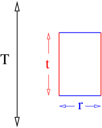
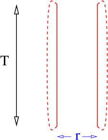
Figure 2: Wilson loop (left) and correlator of Polyakov loops (right).

On the lattice the static potential can be extracted from Wilson loops, which are shown on the left of Fig. 2. A planar Wilson loop is defined as the trace of the product of gauge links along a rectangle of size $r\times t$

$$W(r,t)=\mathrm{tr}\,\left\{P(0,\underline{0};0,r\hat{k})P(0,r\hat{k};t,r\hat{k})P^{\dagger}(t,\underline{0};t,r\hat{k})P^{\dagger}(0,\underline{0};t,\underline{0})\right\}\,.$$ (31)

Here $P(x_{0},\underline{0};x_{0},r\hat{k})$ is the product of spatial links joining the static sources at time $x_{0}$. It represents a string-like state. $P^{\dagger}(0,\underline{x};t,\underline{x})$ is the product of temporal links at position $\underline{x}$. It represents the propagator of the static quark. Assuming that the theory has an (effective) transfer matrix the expectation value of the Wilson loop has the spectral representation

$$\left\langle W(r,t)\right\rangle \stackrel{{\scriptstyle t\to\infty}}{{\sim}} \sum_{n}c_{n}c_{n}^{*}{\rm e}^{-V_{n}(r)t}\,.$$ (32)

This representation is for example derived explicitely in Appendix B of [41]. In pure gauge theory for large values of $r$ and $t$ one expects an area law $\left\langle W(r,t)\right\rangle\sim{\rm e}^{-\sigma rt}$.

The standard way to extract the energy levels $V_{n}$ from eq. (32) is to use some technique of gauge link smearing to replace the spatial lines in the Wilson loops by $P_{i}(x_{0},\vec{0};x_{0},r\hat{k})$, where $i$ is the smearing index. One then has a correlation matrix $\left\langle W_{ij}(r,t)\right\rangle$ (the smearing index $i$ refers to time $0$ and $j$ to time $t$. For fixed distance $r$ the correlation matrix $C_{ij}(t)=\left\langle W_{ij}(r,t)\right\rangle$ is used to build the generalized eigenvalue problem

$$C(t)v_{n}(t,t_{0})=\lambda_{n}(t,t_{0})C(t_{0})v_{n}(t,t_{0})\,,\quad\lambda_{n}>\lambda_{n+1}$$ (33)

The energy levels $V_{n}$ can be computed as [42]

$$V_{n}(r)=-\frac{1}{a}\ln\left\{\frac{\lambda_{n}(t+a,t_{0})}{\lambda_{n}(t,t_{0})}\right\}+\epsilon_{n}(t,t_{0})$$ (34)

with exponential corrections $\epsilon_{n}={\rm O}({\rm e}^{-\Delta E_{n}t})$. We refer to [43] for a derivation of the corrections $\Delta E_{n}$.

The static potential can also be extracted from the spatial correlator of temporal Polyakov loops, which is shown on the right of Fig. 2:

$$P(x)^{*}P(y)|_{y=x+r\hat{k}}\,,$$ (35)

where the Polyakov loop is defined as the trace of the path through $x$ which winds once around the time axis $P(x)=\mathrm{tr}\,\{U_{\mu}(x)U_{\mu}(x+a\hat{\mu})\ldots U_{\mu}(x+(T-a)\hat{\mu})\}|_{\mu=0}$. The static potential is obtained as [47]

$$V(r) \stackrel{{\scriptstyle T\to\infty}}{{\sim}} -\frac{1}{T}\ln\left\langle P(x)^{*}P(y\right\rangle|_{y=x+r\hat{k}}\,.$$ (36)

Using the Polyakov loop correlator requires simulations of lattices with different temporal extents $T$ to take the limit $T\to\infty$.

Wilson loops are not good operators when it comes to compute the static potential in QCD with dynamical quarks (in the fundamental representation of $SU(3)$) at large distances $r$. As we mentioned above at large $r$ due to string breaking the ground state potential is the energy of two static-light mesons which results in a flattening of the static potential. As it was shown in previous studies in the case of the $SU(2)$ Higgs model [49, 50, 51] and then in QCD [52], in order to see string breaking and the flattening of the potential one has to construct a matrix correlation which includes Wilson loops, off-diagonal matrix elements describing the transition between a string-like state and a state made of two static-light mesons and a diagonal element describing only two static-light mesons. Schematically the matrix is represented as

$$\left(\begin{array}[]{rl}\quad\mbox{ \begin{minipage}{24.0pt}\includegraphics[width=24.0pt]{figs/w11}\end{minipage}}&\quad\sqrt{N_{\mathrm{f}}}\mbox{ \begin{minipage}{24.0pt}\includegraphics[width=24.0pt]{figs/w12}\end{minipage}}\\ &\\ \sqrt{N_{\mathrm{f}}}\mbox{ \begin{minipage}{24.0pt}\includegraphics[width=24.0pt]{figs/w21}\end{minipage}}&\quad-N_{\mathrm{f}}\mbox{ \begin{minipage}{24.0pt}\includegraphics[width=24.0pt]{figs/w22c}\end{minipage}}+\mbox{ \begin{minipage}{24.0pt}\includegraphics[width=24.0pt]{figs/w22d}\end{minipage}}\end{array}\right)\,,$$ (37)

where $N_{\mathrm{f}}$ degenerate dynamical quarks are assumed and the diagrams are from [52].

Due to confinement, the Wilson loop has a signal which decays exponentially with the area of the loop: $\left\langle W(r,t)\right\rangle\approx\exp(-\sigma rt)$. This is the result of cancellations in the average between positive and negative values of the loop. The variance of the Wilson loop is instead dominated by $\left\langle W(r,t)^{2}\right\rangle$ which is approximately a constant (being the average of positive values). Therefore the signal-to-noise ratio of Wilson loops decays exponentially with the area of the loop. The same problem arises with Polyakov loops. The deterioration of the quality of the signal can be tamed by the following techniques:

• In pure $SU(N)$ theory, an exponential reduction with the temporal extent $t$ of the error of Wilson loops can be achieved by using the one-link integral to replace the temporal link [44]. An even more effective technique to reduce exponentially the error of the Polyakov loop correlator is the multilevel algorithm [45]. These methods are not applicable with fermions.

• With fermions, HYP smearing [46] can be used to smear the temporal gauge links in the Wilson loops [40]. This minimizes the self-energy contribution of the static quarks and therefore improves the signal-to-noise ratio [48]. Still the signal-to-noise ratio falls off exponentially.

Smearing is also applied to the quark fields in the correlation matrix eq. (37) to improve the overlap with the physical states. An efficient quark smearing technique is distillation [53].

4.3 Lattice results

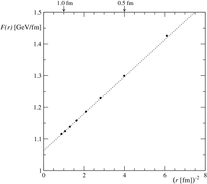
Figure 3: Left: the static potential in the pure gauge theory, from [57]. Right: the static force in the pure gauge theory, from [47].

The static potential can be used to define a physical scale by solving the following equation for the static force

$$r^{2}F(r)|_{r=r(c)}=c\,.$$ (38)

Specifying a value for the constant $c$ and solving for $r=r(c)$ leads to a value $r(c)/a$ in lattice units. If $r(c)$ is known in physical units of $\mathrm{fm}$ (fermi) the lattice spacing can be determined. Taking $c=1.65$ leads to the Sommer scale $r_{0}=r(1.65)$ which has a value of about $0.5\,\mathrm{fm}$ in QCD [54]. The physical value can be determined by comparing to phenomenological potential models. Alternatively it can be extracted by computing the product with another scale, for example with the kaon decay constant $r_{0}f_{\rm K}$ and using the physical value of $f_{\rm K}$, see [55]. Other choices for $c$ in eq. (38) are $r_{1}=r(1.0)$ [56] and $r_{c}=r(0.65)$ [57].

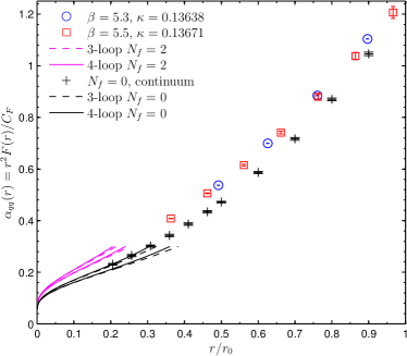
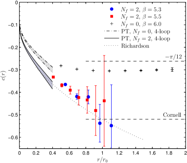
Figure 4: Left: the running coupling $\alpha_{\rm qq}(1/r)$ in the $N_{\mathrm{f}}=2$ theory compared to perturbation theory and $N_{\mathrm{f}}=0$ data from [57]. Right: the slope of the static force $c(r)$, which is proportional to a running coupling, compared to pertutbation theory, potential models and $N_{\mathrm{f}}=0$ data from [47]. The plots are taken from [58].

In this section we present a selection of results about the static potential obtained from lattice simulations which illustrate fundamental properties of QCD. In Fig. 3 we show results for the static potential (left) and the static force (right) in the pure gauge theory. The left plot is taken from [57] and shows the static potential after taking the continuum limit (black circles). At short distances it is compared to the perturbative expansion (continued line). The latter is computed from the static force by integrating the renormalization group equation for $\alpha_{\rm qq}$ as in eq. (29) with the 3-loop $\beta$-function (i.e. using the coefficients of the $\beta_{\mathrm{qq}}$ function up to and including $b^{\rm(qq)}_{2}$ in eq. (28)). The dotted line is the parameter free prediction from the bosonic string in eq. (30), where the string tension is fixed by $\sigma r_{0}^{2}=1.65-\pi/12$. One sees that the bosonic string model agrees very well with the data for the static potential already at distances around $r_{0}$. This is confirmed by the right plot in Fig. 3, which is taken from [47] and shows the static force as a function of $1/r^{2}$. The bosonic string predicts $F(r)=\sigma-\gamma/r^{2}+{\rm O}(1/r^{4})$. Indeed the data are well approximated by a linear function in $1/r^{2}$ (dotted line, fitted to the four points at the largest distances) as soon as $r\geq r_{0}\simeq 0.5\,\mathrm{fm}$. Still there is a curvature in the data which can be measured by computing the slope

$$c(r)=\frac{1}{2}r^{3}F^{\prime}(r)\,,$$ (39)

which is shown in the right plot of Fig. 4. The slope $c(r)$ can be used to define a running coupling $\alpha_{\rm c}=\bar{g}_{\mathrm{c}}^{2}/(4\pi)$ for small $r$

$$\alpha_{\rm c}(\mu)=-\frac{1}{C_{\rm F}}c(r)$$ (40)

at the renormalization $\mu=1/r$. The beta function for the coupling $\alpha_{\rm c}$ can be found in Appendix B of [40].

The coupling $\alpha_{\rm qq}$ and the slope $c(r)$ have been measured in the theory with $N_{\mathrm{f}}=2$ dynamical fermions. The results are shown in Fig. 4. We used the ensembles of gauge configurations labelled “F7” and “O7” in [55] which were generated by CLS (Coordinated Lattice Simulations consortium) using the Wilson gauge action and $N_{\mathrm{f}}=2$ flavors of O($a$) improved Wilson quarks. The lattice spacings are $a=0.066\,\mathrm{fm}$ (blue circles) and $a=0.049\,\mathrm{fm}$ (red squares) and the quark mass corresponds to a pion mass $m_{\pi}=270\,\mathrm{MeV}$. In Fig. 4 we also plot the perturbative curves obtained from eq. (29) (and a similarly for the coupling $\bar{g}_{\mathrm{c}}$). The $\Lambda$ parameters are known from [59] for the $N_{\mathrm{f}}=0$ theory and from [55] for the $N_{\mathrm{f}}=2$ theory. The band of the perturbative curves reflects the uncertainty of the $\Lambda$ parameter. A quantitative comparison to the perturbative curves requires a careful continuum limit and, certainly for the $N_{\mathrm{f}}=2$ theory, smaller lattice spacings to reach small enough distances $r$. In the right plot about $c(r)$ in Fig. 4 we compare the $N_{\mathrm{f}}=2$ data to the value $c=-0.52$ (dashed line) that it takes in the phenomenological Cornell potential [60] and to the curve (dotted) derived from the Richardson potential [61]. The slope $c$ is an interesting but difficult quantity for holographic QCD models [62].

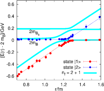
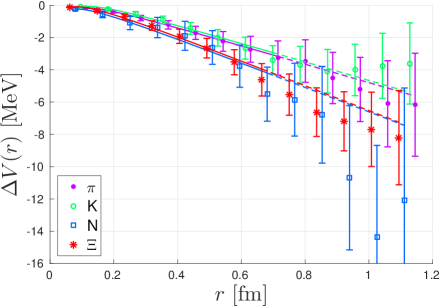
Figure 5: Left plot: the static potential (red circles) and its first excited state (blue pentagrams), from [52]. Right plot: the modification of the static potential in the presence of a hadrons, from [65].

The energy levels for the ground state and the first excited state potentials in QCD with $N_{\mathrm{f}}=2$ dynamical quarks have been calculated in [52] from the correlation matrix eq. (37). The simulations are done at a lattice spacing $a=0.083\,\mathrm{fm}$ and pion mass $m_{\pi}=400\,\mathrm{MeV}$ and the results are shown in the left plot of Fig. 5. The string breaking distance was calculated to be $r_{\mathrm{b}}/r_{0}\approx 2.5$. The cyan bands are a qualitative sketch of the expected behavior with $N_{\mathrm{f}}=2+1$ dynamical quarks, where a second breaking happens. Calculations of string breaking with $N_{\mathrm{f}}=2+1$ are under way [63]. The continuum limit and the dependence on the quark mass of string breaking are still open issues. String breaking is a fundamental aspect of QCD with dynamical quarks. It provides input for phenomenological potential models which can shed light on the nature of recently-discovered exotic heavy-flavor hadrons, see [64] for a recent discussion.

The static potential is modified by the presence of a hadron. The difference $\Delta V_{H}=V_{H}-V_{0}$ of the static potential in the presence of a hadron $V_{H}$ and the static potential in the vacuum $V_{0}$ can be computed from the correlator of a Wilson loop $W(r,t)$ and a hadron two-point function $C_{H,\mathrm{2pt}}$ defined as [65]

$$C_{H}(r,\delta t,t)=\frac{\langle W(r,t)C_{H,\mathrm{2pt}}(t+2\delta t)\rangle}{\langle W(r,t)\rangle\langle C_{H,\mathrm{2pt}}(t+2\delta t)\rangle}\,.$$ (41)

The argument $\delta t$ is the distance in time between the source of the hadron and the Wilson loop and it is also the same distance between the latter and the sink of the hadron (i.e. the hadron propagates over a time $t+2\delta t$). The potential difference is computed as $\Delta V_{H}=-\lim_{t\rightarrow\infty}\frac{{\rm d}}{{\rm d}t}\ln[C_{H}(r,\delta t,t)]$ and extrapolating $\delta t\to\infty$. The right plot of Fig. 5 presents the results for the shift $\Delta V_{H}$ for the pion $\pi$, the kaon $K$, the nucleon $N$ and the cascade $\Xi$. The calculation was done using the $N_{\mathrm{f}}=2+1$ ensemble of gauge configurations labelled “C101” generated by CLS [66]. The lattice spacing is $a=0.0854(15)\,\mathrm{fm}$ and the kaon and pion masses are $m_{\pi}\approx 223\,\mathrm{MeV}$ and $m_{\mathrm{K}}\approx 476\mathrm{MeV}$ respectively. The potential shift is negative and of similar size for all hadrons investigated. The effect is small, it is $-\Delta V_{H}\approx 2$–$3\,\mathrm{MeV}$ at distance $r=0.5\,\mathrm{fm}\simeq r_{0}$. Solving the Schrödinger equation with the modified potential yields a stronger binding of charmonium states ($c\bar{c}$). Their masses decrease by few MeV like the binding of deuterium. The modification of the static potential in the presence of a hadron is a test of the idea of hadro-quarkonia [67] which provides a possible interpretation for the candidates of a penta-quark state ($c\bar{c}uud$) reported in [68, 69].

5 Conclusions

More than 40 years after its invention, lattice QCD has developed into an active field of research connecting physics, mathematics and informatics. As it was shown in this lecture using the example of the static potential, there are still important open questions to be answered.

Acknowledgments. I thank Peter Weisz for his help in providing me with his lecture at the Corfu Summer School 2014 and Tomasz Korzec for his valuable comments on the manuscript. I acknowledge financial support from the Program for European Joint Doctorates HPC-LEAP (High Performance Computing in Life sciences, Engineering and Physics).

References

- [1] F. Knechtli, M. Günther and M. Peardon, Lattice Quantum Chromodynamics: Practical Essentials, doi:10.1007/978-94-024-0999-4.
- [2] M. Lüscher, Lattice QCD: From quark confinement to asymptotic freedom, Annales Henri Poincare 4 (2003) S197, [hep-ph/0211220].
- [3] D. J. Gross and F. Wilczek, Ultraviolet Behavior of Nonabelian Gauge Theories, Phys. Rev. Lett. 30 (1973) 1343.
- [4] H. D. Politzer, Reliable Perturbative Results for Strong Interactions?, Phys. Rev. Lett. 30 (1973) 1346.
- [5] C. Patrignani et al. [Particle Data Group], Review of Particle Physics, Chin. Phys. C 40 (2016) no.10, 100001.
- [6] K. G. Wilson, Confinement of Quarks, Phys. Rev. D 10 (1974) 2445.
- [7] K. G. Wilson, The Origins of lattice gauge theory, Nucl. Phys. Proc. Suppl. 140 (2005) 3, [hep-lat/0412043].
- [8] B. Sheikholeslami and R. Wohlert, Improved Continuum Limit Lattice Action for QCD with Wilson Fermions, Nucl. Phys. B 259 (1985) 572.
- [9] G. Heatlie, G. Martinelli, C. Pittori, G. C. Rossi and C. T. Sachrajda, The improvement of hadronic matrix elements in lattice QCD, Nucl. Phys. B 352 (1991) 266.
- [10] P. H. Ginsparg and K. G. Wilson, A Remnant of Chiral Symmetry on the Lattice, Phys. Rev. D 25 (1982) 2649.
- [11] P. Hasenfratz, V. Laliena and F. Niedermayer, The Index theorem in QCD with a finite cutoff, Phys. Lett. B 427 (1998) 125, [hep-lat/9801021].
- [12] M. Lüscher, Exact chiral symmetry on the lattice and the Ginsparg-Wilson relation, Phys. Lett. B 428 (1998) 342, [hep-lat/9802011].
- [13] H. Neuberger, Exactly massless quarks on the lattice, Phys. Lett. B 417 (1998) 141, [hep-lat/9707022].
- [14] C. Gattringer and C. B. Lang, Quantum chromodynamics on the lattice, Lect. Notes Phys. 788 (2010) 1.
- [15] M. Lüscher, Construction of a Selfadjoint, Strictly Positive Transfer Matrix for Euclidean Lattice Gauge Theories, Commun. Math. Phys. 54 (1977) 283.
- [16] R. Sommer, Scale setting in lattice QCD, PoS LATTICE 2013 (2014) 015, [arXiv:1401.3270 [hep-lat]].
- [17] K. Symanzik, Cutoff dependence in lattice theory, NATO Sci. Ser. B 59 (1980) 313.
- [18] P. Weisz, Renormalization and lattice artifacts, [arXiv:1004.3462].
- [19] M. Lüscher, Computational Strategies in Lattice QCD, [arXiv:1002.4232 [hep-lat]].
- [20] M. Lüscher, A Portable high quality random number generator for lattice field theory simulations, Comput. Phys. Commun. 79 (1994) 100, [hep-lat/9309020].
- [21] U. Wolff [ALPHA Collaboration], Monte Carlo errors with less errors, Comput. Phys. Commun. 156 (2004) 143, Erratum: [Comput. Phys. Commun. 176 (2007) 383], [hep-lat/0306017].
- [22] S. Duane, A. D. Kennedy, B. J. Pendleton and D. Roweth, Hybrid Monte Carlo, Phys. Lett. B 195 (1987) 216.
- [23] S. Schaefer et al. [ALPHA Collaboration], Critical slowing down and error analysis in lattice QCD simulations, Nucl. Phys. B 845 (2011) 93, [arXiv:1009.5228 [hep-lat]].
- [24] M. Lüscher and S. Schaefer, Lattice QCD without topology barriers, JHEP 1107 (2011) 036, [arXiv:1105.4749 [hep-lat]].
- [25] W. Fischler, Quark - anti-Quark Potential in QCD, Nucl. Phys. B 129 (1977) 157.
- [26] A. Billoire, How Heavy Must Be Quarks in Order to Build Coulombic q anti-q Bound States, Phys. Lett. 92B (1980) 343.
- [27] M. Peter, The Static potential in QCD: A Full two loop calculation, Nucl. Phys. B 501 (1997) 471, [hep-ph/9702245].
- [28] Y. Schroder, The Static potential in QCD to two loops, Phys. Lett. B 447 (1999) 321, [hep-ph/9812205].
- [29] M. Melles, The Static QCD potential in coordinate space with quark masses through two loops, Phys. Rev. D 62 (2000) 074019, [hep-ph/0001295].
- [30] N. Brambilla, A. Pineda, J. Soto and A. Vairo, Potential NRQCD: An Effective theory for heavy quarkonium, Nucl. Phys. B 566 (2000) 275, [hep-ph/9907240].
- [31] N. Brambilla, A. Pineda, J. Soto and A. Vairo, The Infrared behavior of the static potential in perturbative QCD, Phys. Rev. D 60 (1999) 091502, [hep-ph/9903355].
- [32] A. V. Smirnov, V. A. Smirnov and M. Steinhauser, Three-loop static potential, Phys. Rev. Lett. 104 (2010) 112002, [arXiv:0911.4742 [hep-ph]].
- [33] C. Anzai, Y. Kiyo and Y. Sumino, Static QCD potential at three-loop order, Phys. Rev. Lett. 104 (2010) 112003, [arXiv:0911.4335 [hep-ph]].
- [34] R. N. Lee, A. V. Smirnov, V. A. Smirnov and M. Steinhauser, Analytic three-loop static potential, Phys. Rev. D 94 (2016) no.5, 054029, [arXiv:1608.02603 [hep-ph]].
- [35] Y. Nambu, QCD and the String Model, Phys. Lett. 80B (1979) 372.
- [36] M. Lüscher, K. Symanzik and P. Weisz, Anomalies of the Free Loop Wave Equation in the WKB Approximation, Nucl. Phys. B 173 (1980) 365.
- [37] M. Lüscher, Symmetry Breaking Aspects of the Roughening Transition in Gauge Theories, Nucl. Phys. B 180 (1981) 317.
- [38] M. Lüscher and P. Weisz, String excitation energies in SU(N) gauge theories beyond the free-string approximation, JHEP 0407 (2004) 014, [hep-th/0406205].
- [39] M. Lüscher, G. Münster and P. Weisz, How Thick Are Chromoelectric Flux Tubes?, Nucl. Phys. B 180 (1981) 1.
- [40] M. Donnellan, F. Knechtli, B. Leder and R. Sommer, Determination of the Static Potential with Dynamical Fermions, Nucl. Phys. B 849 (2011) 45, [arXiv:1012.3037 [hep-lat]].
- [41] F. Knechtli, The Static potential in the SU(2) Higgs model, [hep-lat/9910044].
- [42] M. Lüscher and U. Wolff, How to Calculate the Elastic Scattering Matrix in Two-dimensional Quantum Field Theories by Numerical Simulation, Nucl. Phys. B 339 (1990) 222.
- [43] B. Blossier, M. Della Morte, G. von Hippel, T. Mendes and R. Sommer, On the generalized eigenvalue method for energies and matrix elements in lattice field theory, JHEP 0904 (2009) 094, [arXiv:0902.1265 [hep-lat]].
- [44] G. Parisi, R. Petronzio and F. Rapuano, A Measurement of the String Tension Near the Continuum Limit, Phys. Lett. 128B (1983) 418.
- [45] M. Lüscher and P. Weisz, Locality and exponential error reduction in numerical lattice gauge theory, JHEP 0109 (2001) 010, [hep-lat/0108014].
- [46] A. Hasenfratz and F. Knechtli, Flavor symmetry and the static potential with hypercubic blocking, Phys. Rev. D 64 (2001) 034504, [hep-lat/0103029].
- [47] M. Lüscher and P. Weisz, Quark confinement and the bosonic string, JHEP 0207 (2002) 049, [hep-lat/0207003].
- [48] M. Della Morte, A. Shindler and R. Sommer, On lattice actions for static quarks, JHEP 0508 (2005) 051, [hep-lat/0506008].
- [49] F. Knechtli and R. Sommer [ALPHA Collaboration], String breaking in SU(2) gauge theory with scalar matter fields, Phys. Lett. B 440 (1998) 345, Erratum: [Phys. Lett. B 454 (1999) 399], [hep-lat/9807022].
- [50] F. Knechtli and R. Sommer [ALPHA Collaboration], String breaking as a mixing phenomenon in the SU(2) Higgs model, Nucl. Phys. B 590 (2000) 309, [hep-lat/0005021].
- [51] O. Philipsen and H. Wittig, String breaking in nonAbelian gauge theories with fundamental matter fields, Phys. Rev. Lett. 81 (1998) 4056, Erratum: [Phys. Rev. Lett. 83 (1999) 2684] [hep-lat/9807020].
- [52] G. S. Bali, H. Neff, T. Düssel, T. Lippert and K. Schilling [SESAM Collaboration], Observation of string breaking in QCD, Phys. Rev. D 71 (2005) 114513, [hep-lat/0505012].
- [53] M. Peardon, J. Bulava, J. Foley, C. Morningstar, J. Dudek, R. G. Edwards, B. Joo, H. W. Lin, D. G. Richards, K. J. Juge [Hadron Spectrum Collaboration], A Novel quark-field creation operator construction for hadronic physics in lattice QCD, Phys. Rev. D 80 (2009) 054506, [arXiv:0905.2160 [hep-lat]].
- [54] R. Sommer, A New way to set the energy scale in lattice gauge theories and its applications to the static force and alpha-s in SU(2) Yang-Mills theory, Nucl. Phys. B 411 (1994) 839, [hep-lat/9310022].
- [55] P. Fritzsch, F. Knechtli, B. Leder, M. Marinkovic, S. Schaefer, R. Sommer and F. Virotta, The strange quark mass and Lambda parameter of two flavor QCD, Nucl. Phys. B 865 (2012) 397, [arXiv:1205.5380 [hep-lat]].
- [56] C. W. Bernard, T. Burch, K. Orginos, D. Toussaint, T. A. DeGrand, C. E. DeTar, S. A. Gottlieb, U. M. Heller, J. E. Hetrick and B. Sugar, The Static quark potential in three flavor QCD, Phys. Rev. D 62 (2000) 034503, [hep-lat/0002028].
- [57] S. Necco and R. Sommer, The N(f) = 0 heavy quark potential from short to intermediate distances, Nucl. Phys. B 622 (2002) 328, [hep-lat/0108008].
- [58] B. Leder and F. Knechtli [ALPHA Collaboration], The shape of the static potential with dynamical fermions, PoS LATTICE 2011 (2011) 315, [arXiv:1112.1246 [hep-lat]].
- [59] S. Capitani, M. Lüscher, R. Sommer and H. Wittig, Non-perturbative quark mass renormalization in quenched lattice QCD, Nucl. Phys. B 544 (1999) 669, Erratum: [Nucl. Phys. B 582 (2000) 762], [hep-lat/9810063].
- [60] E. Eichten, K. Gottfried, T. Kinoshita, K. D. Lane and T. M. Yan, Charmonium: Comparison with Experiment, Phys. Rev. D 21 (1980) 203.
- [61] J. L. Richardson, The Heavy Quark Potential and the Upsilon, J/psi Systems, Phys. Lett. 82B (1979) 272.
- [62] D. Giataganas and N. Irges, Flavor Corrections in the Static Potential in Holographic QCD, Phys. Rev. D 85 (2012) 046001, [arXiv:1104.1623 [hep-th]].
- [63] V. Koch, J. Bulava, B. Hörz, F. Knechtli, G. Moir, C. Morningstar and M. Peardon, Towards string breaking with 2+1 dynamical fermions using the stochastic LapH method, PoS LATTICE 2015 (2016) 100, [arXiv:1511.04029 [hep-lat]].
- [64] R. Oncala and J. Soto, Heavy Quarkonium Hybrids: Spectrum, Decay and Mixing, arXiv:1702.03900 [hep-ph].
- [65] M. Alberti, G. S. Bali, S. Collins, F. Knechtli, G. Moir and W. Söldner, Hadroquarkonium from lattice QCD, Phys. Rev. D 95 (2017) no.7, 074501, [arXiv:1608.06537 [hep-lat]].
- [66] M. Bruno et al., Simulation of QCD with N 2 1 flavors of non-perturbatively improved Wilson fermions, JHEP 1502 (2015) 043, [arXiv:1411.3982 [hep-lat]].
- [67] S. Dubynskiy and M. B. Voloshin, Hadro-Charmonium, Phys. Lett. B 666 (2008) 344, [arXiv:0803.2224 [hep-ph]].
- [68] R. Aaij et al. [LHCb Collaboration], Observation of Resonances Consistent with Pentaquark States in Decays, Phys. Rev. Lett. 115 (2015) 072001, [arXiv:1507.03414 [hep-ex]].
- [69] R. Aaij et al. [LHCb Collaboration], Model-independent evidence for contributions to decays, Phys. Rev. Lett. 117 (2016) no.8, 082002, [arXiv:1604.05708 [hep-ex]].