Tidal Forces in Kiselev Black Hole

Abstract

The aim of this paper is to examine the tidal forces occurred in Kiselev black hole surrounded by radiation and dust fluids. It is noted that radial and angular component of tidal force change the sign between event and Cauchy horizons. We solve the geodesic deviation equation for radially free falling bodies toward Kiselev black holes. We explain the geodesic deviation vector graphically and point out the location of event and Cauchy horizons in it for specific values of radiation and dust parameter.

1 Introduction

At present, type 1a supernova [1], Cosmic microwave background (CMB) radiation [2] and large scale structure [3, 4] have shown that our universe is currently in accelerating expansion period. Dark energy is responsible for this acceleration and it has strange property that violates the null energy condition (NEC) and weak energy condition (WEC) [5, 6] and produces strong repulsive gravitational effects. Recent observations suggests that approximately 74% of our universe is occupied by dark energy and the rest 22% and 4% is of dark matter and ordinary matter respectively. Nowadays dark energy is the most challenging problem in astrophysics. Many theories have been proposed to handle this important problem in last two decade.

With the discovery of cosmic acceleration, black holes (BHs) phenomenon have become the most fascinating in illustrating their significant physical properties. There exists two major types of vacuum BH solutions in general relativity, i.e., uncharged (for example Schwarzschild BH) and charged (for example Reissner-Nordstrom BH). These BHs have been thoroughly investigated by many authors over the years. For example, there exists a well-known phenomena in which a body experiences compression in angular direction and stretching in radial direction when it falls toward the event horizon of uncharged static BHs [7, 8, 9, 10, 11]. However, in Reissner-Nordstrom BH, a body may experience stretching in radial direction and compression in angular direction depends upon two phenomenons $1)$ the location of body and $2)$ charge to mass ratio of BH [12]. Tidal forces change their sign in radial or angular direction at certain points of Reissner-Nordstrom BH unlike Schwarzschild BH. Geodesics deviation of Schwarzschild and Reissner-Nordstrom space-times are studied in detail by [13, 7, 12, 14, 15]. Ghosh and Kerr [16] discussed geodesics deviation and geodesic motion in wrapped space-time with extra dimension of time. It is also realized that the geodesics deviation needs to analyze using full general relativity on the other hand tidal forces can be found with Newtonian mechanics if an extra force coming from general relativity is added.

However, several BHs of Einstein general relativity in non-vacuum case have also been presented [17, 18, 19, 20, 21, 22] which need more physical illustrations. One of them is Kiselev BH which possesses new set of phenomena unlike Schwarzschild BH because of the important complex properties [22] and this BH has been surrounded by various types of matter depending on state parameter $\omega$. Kiselev BH have been investigated through various phenomenon, i.e., accretion [23], strong gravitational lensing [24], thermodynamics and phase transition [25]. In this work, we apply the technique of [26] on the solution of Kiselev BH surrounded by energy matter i.e. we consider Kiselev BH surrounded by dust and radiation parameter derived by Kiselev [22], in which we consider non zero electric charge, dust and radiation parameter but no angular momentum. They are exact solutions of Einstein Maxwell equation [13], in the case of vanishing dust and radiation parameter it reduces to RN space time and in the case of vanishing electric charge it reduces to SH space time.

In this paper we discuss the tidal forces in Kiselev space-time and consider its two cases which leads to Kiselev space-time surrounded by dust $(\omega=0)$ and radiation $(\omega=1/3)$. We solve the geodesic deviation equations to observe the variation of test body in-falling radially toward the Kiselev BH for specific choices of dust and radiation parameter. This paper is organized as follows: In Sect. 2, we discuss Kiselev BHs, its two special cases and radial geodesics. In Sect. 3, we derive the tidal forces in Kiselev space-time on a neutral body in radial free fall. In Sect. 4, we find the solutions of the geodesic equations in Kiselev space-time. In the end, we conclude our results. In this paper, we use the metric signature (+, -, -, -) and set the speed of light $c$ and Newtonian gravitational constant $G$ to $1$.

2 Kiselev black holes and its two special cases

The line element of static charged BH surrounded by energy-matter is given by

$$ds^{2}=f(r)dt^{2}-f(r)^{-1}dr^{2}-r^{2}({d\theta}^{2}+\sin\theta{d\phi}^{2}),$$ (1)

with

$$f(r)=1-\frac{2M}{r}+\frac{q^{2}}{r^{2}}-\frac{\sigma}{r^{3\omega+1}},$$ (2)

where $M$ and $q$ are the mass and electric charge, $\sigma$ and $\omega$ are normalization parameter and state parameter of matter around BH, respectively [22]. We assume $\omega=1/3$ which becomes Kiselev BH surrounded by radiation and $\omega=0$ Kiselev BH surrounded by dust. For Kiselev BH surrounded by radiation, the radial coordinated of horizons are obtained by taking $f(r)=0$, i.e.

$$r_{\pm} = M+\sqrt{M^{2}-q^{2}+\sigma_{r}},$$ (3)

where $\sigma_{r}$ is parameter of radiation. We will assume only the cases in which $M^{2}-q^{2}+\sigma_{r}\geq 0$ because naked singularities ($M^{2}-q^{2}+\sigma_{r}<0$) do not occur in nature if the cosmic conjecture is true. Eq. (3) give the location of event as well as Cauchy horizon of BH, respectively.

Similarly, for Kiselev BH surrounded by dust ($\omega=0$), the radial coordinated of horizons are

$$r_{\pm} = \frac{2M+\sigma_{d}\pm\sqrt{(2M+\sigma_{d})^{2}-4q^{2}}}{2},$$ (4)

where $\sigma_{d}$ is parameter of dust. We choose the case in which $(2M+\sigma_{d})^{2}\geq 4q^{2}$ because naked singularities ($(2M+\sigma_{d})^{2}<4q^{2}$) do not occur in nature if the cosmic conjecture is true [27]. Eq. (4) give the location of event as well as Cauchy horizon of the BH, respectively [22].

2.1 Radial Geodesics

Radial geodesic motion for line element (1) in sphereically symmetric spacetimes is obtained by considering $ds=d\tau$ in Eq. (1), which is [28]

$$f(r)\dot{t}^{2}-f(r)^{-1}\dot{r}^{2}=1,$$ (5)

where dot represents the derivative with respect to proper time $\tau$. Because of the assumption of radial motion, we have $\dot{\theta}=\dot{\phi}=0$. $E=f(r)\dot{t}$ is well known conserved energy. By putting this in Eq. (4), we have

$$\frac{\dot{r}^{2}}{2}=\frac{E^{2}-f(r)}{2}.$$ (6)

For the radial infall of a test particle from rest at position $b$, we get $E=\sqrt{f(r=b)}$ from Eq. (6) [29]. Newtonian radial acceleration is defined by [30]

$$A^{R}=\ddot{r},$$ (7)

Using Eqs.(6) and (7), we obtain

$$A^{R}=-\frac{f^{\prime}(r)}{2},$$ (8)

where prime represents the derivative with respect to $r$ (radial coordinate). For Kiselev BH surrounded by radiation and dust, we obtain

$$A_{r}^{R}=-\frac{M}{r^{2}}+\frac{q^{2}}{r^{3}}-\frac{\sigma_{r}}{r^{3}},\quad A_{d}^{R}=-\frac{M}{r^{2}}+\frac{q^{2}}{r^{3}}-\frac{\sigma_{d}}{r^{2}}.$$ (9)

The terms $\frac{q^{2}}{r^{3}}-\frac{\sigma_{r}}{r^{3}}$ and $\frac{q^{2}}{r^{3}}-\frac{\sigma_{d}}{r^{2}}$ in Eq. (9) represents the purely relativistic effect. Eq. (9) explain the ”exertion” of Kiselev space-time surrounded by radiation and dust on a neutral free falling of massive test body. Interestingly, free fall test particle from rest at $r=b$ (for $q,\sigma_{r},\sigma_{d}\neq 0$) would bounce back at radius $R^{stop}$. The radius $R^{stop}$ for Kiselev space-time surrounded by radiation ($R_{r}^{stop}$) and dust ($R_{d}^{stop}$) could be found as

$$R_{r}^{stop} = \frac{b(q^{2}-\sigma_{r})}{2Mb-q^{2}+\sigma_{r}},$$ (10)

$$R_{d}^{stop} = \frac{b~{}q^{2}}{(2Mb+b\sigma_{d}-q^{2})},$$ (11)

where $b$ is the initial position starting from rest of test particle. $R^{stop}$ located inside the Cauchy (internal) horizon. One can find in the limit $b\rightarrow\infty$, $R_{r}^{stop}\rightarrow(q^{2}-\sigma_{r})/2M$ for radiation and $R_{d}^{stop}\rightarrow q^{2}/(2M-\sigma_{d})$ for dust. The particle in Kiselev BH surrounded by radiation and dust would emerge in different asymptotically flat region in maximal analytic extension. Thus, the particle is physically unstable in maximal analytic extension beyond the internal (Cauchy) horizons of Kiselev space-time surrounded by radiation and dust.

3 Tidal forces in Kiselev space-time on a neutral body in radial free fall

The equation for the space-like components of the geodesic deviation vector $\zeta^{\alpha}$ that describes the distance between two infinitesimally close particles in free fall is given by [7, 8]

$$\frac{D^{2}\zeta^{\alpha}}{D\tau^{2}}-R^{\alpha}_{\beta\gamma\delta}v^{\beta}v^{\gamma}\zeta^{\delta}=0,$$ (12)

where $v^{\gamma}$ is the unit vector tangent to the geodesic. We use the tetrad basis for radial free fall reference frames [26]

$$\hat{e}^{\alpha}_{\hat{0}} = \left(\frac{E}{f(r)},-\sqrt{E^{2}-f(r)},0,0\right),$$ (13)

$$\hat{e}^{\alpha}_{\hat{1}} = \left(\frac{-\sqrt{E^{2}-f(r)}}{f(r)},E,0,0\right),$$ (14)

$$\hat{e}^{\alpha}_{\hat{2}} = r^{-1}(0,0,1,0),$$ (15)

$$\hat{e}^{\alpha}_{\hat{3}} = (r\sin(\theta)^{-1}(0,0,0,1),$$ (16)

where $(x^{0},x^{1},x^{2},x^{3})=(t,r,\theta,\phi)$. These unit vectors satisfy the following orthonomality condition

$$\hat{e}^{\mu}_{\hat{\alpha}}\hat{e}_{\hat{\gamma}\mu}=\zeta_{\hat{\alpha}\hat{\gamma}},$$ (17)

where $\zeta_{\hat{\alpha}\hat{\gamma}}$ is the Minkowski metric [7]. We have $\hat{e}^{\alpha}_{\hat{0}}=v^{\alpha}$. The geodesic deviation vector, also called Jacobi vector, can be written as

$$\zeta^{\alpha}=\hat{e}^{\alpha}_{\hat{\gamma}}\zeta^{\hat{\gamma}}.$$ (18)

Here we note that $\zeta^{\hat{0}}=0$ [7] and $\hat{e}^{\alpha}_{\hat{\gamma}}$ are all parallelly transported vectors along the geodesic.

The non-zero independent components of the Riemann tensor in spherically symmetric space-times are

$$R^{1}_{010} = \frac{f(r)f^{\prime\prime}(r)}{2},R^{1}_{212}=-\frac{rf^{\prime}(r)}{2},R^{1}_{313}=-\frac{rf^{\prime}(r)}{2}\sin^{2}\theta$$

$$R^{2}_{020} = \frac{f(r)f^{\prime}(r)}{2r},R^{2}_{323}=\left(1-f(r)\right)\sin^{2}\theta,R^{3}_{030}=\frac{f(r)f^{\prime}(r)}{2r}.$$

Using above equations in Eq. (12), we find the following equations for radial free fall tidal forces [12]

$$\ddot{\zeta}^{\hat{1}} = -\frac{f^{\prime\prime}}{2}\zeta^{\hat{1}},$$ (19)

$$\ddot{\zeta}^{\hat{i}} = -\frac{f^{\prime}}{2r}\zeta^{\hat{i}},$$ (20)

where $i=2,3$. For aforementioned cases of Kiselev BH, Eqs.(19) and (20) provided that the tidal forces depend on the mass and electric charge of a BH as well as radiation and dust fluid. Tidal forces are identical to Newtonian tidal forces with the force $-\frac{f^{\prime}}{2}$ in radial direction can be observed in Eqs.(19) and (20). Further, we will explore Eqs. (19) and (20) for Kiselev space-time in detail.

3.1 Radial tidal forces

Radial tidal forces vanishes at $r=R^{rtf}_{0}$ (for radiation) and $r=R^{rtf}_{1}$ (for dust) by using Eqs. (19) and (20),

$$R^{rtf}_{0} = \frac{3(q^{2}-\sigma_{r})}{2M},$$ (21)

$$R^{rtf}_{1} = \frac{3q^{2}}{2M+\sigma_{d}}.$$ (22)

The maximum value of radial tidal force is at $R^{rtf}_{0max}$ for radiation and $R^{rtf}_{1max}$ for dust such that

$$R^{rtf}_{0max} = \frac{2(q^{2}-\sigma_{r})}{M},$$ (23)

$$R^{rtf}_{1max} = \frac{2q^{2}}{M+\sigma_{d}}.$$ (24)

The maximum radial stretching for above equations are

$$\ddot{\zeta}^{1}|_{max} = \frac{M^{4}}{16(q^{2}-\sigma_{r})^{4}},$$ (25)

$$\ddot{\zeta}^{1}|_{max} = \frac{(M+\sigma_{d})^{4}}{16q^{6}}.$$ (26)

The radial tidal force using Eqs.(21) and (22) for Kiselev BH surrounded by radiation and dust for different choices of charge is shown in Figures 1 and 2. The local maximum of radial tidal force for radiation is greater as compared to the dust near the singularity.

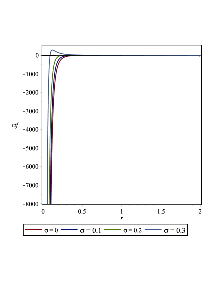
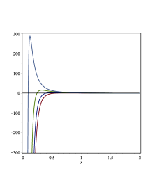
Figure 1: Radial tidal force for Kiselev BH surrounded by radiation for chosen values radiation parameter, also $q=0.6$ and $b=100$.

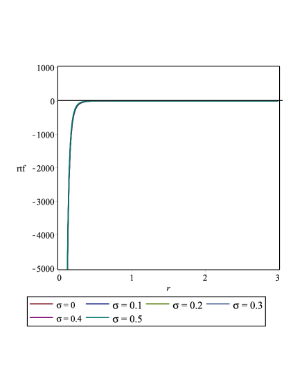
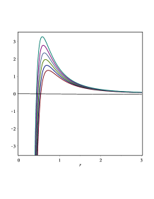
Figure 2: Radial tidal force for Kiselev BH surrounded by dust for chosen values dust parameter, also $q=0.6$, $M=1$ and $b=100$.

3.2 Angular tidal forces

The angular tidal forces vanish at

$$R^{atf}_{0} = \frac{q^{2}-\sigma_{r}}{M},$$ (27)

$$R^{atf}_{1} = \frac{2q^{2}}{(2M+\sigma_{d})},$$ (28)

by using Eqs. (2) and (20) for Kiselev spacetime surrounded by radiation and dust, respectively. Also one can find the following conditions from Eqs. (3), (4), (27) and (28)

$$r_{-} \leq R^{atf}_{0}\leq r_{+},$$ (29)

$$r_{-} \leq R^{atf}_{1}\leq r_{+},.$$ (30)

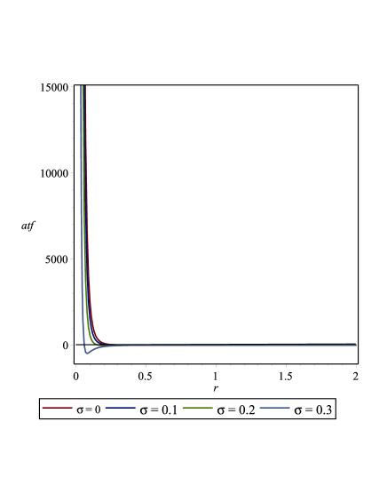
Figure 3: Angular tidal force for Kiselev BH surrounded by radiation for chosen values radiation parameter, also $q=0.6$, $M=1$ and $b=100$.

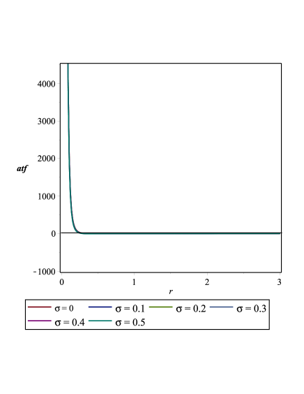
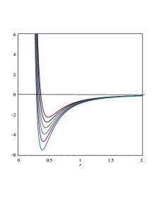
Figure 4: Angular tidal force for Kiselev BH surrounded by dust for chosen values dust parameter, also $q=0.6$ and $b=100$.

On the basis of these relations, it is pointed out here that the angular tidal forces becomes zero at some points between the event horizon and Cauchy horizon. The angular tidal force for different choices of $q$ for Kiselev BH surrounded by radiation and dust is given in Figure 3 and 4. The local minimum of radial tidal force for radiation is greater as compared to the dust near the singularity.

4 Solutions of the geodesic equations for Kiselev BH

We solve the geodesic deviation Eqs.(19) and (20) and find the geodesic deviation vectors as functions of $r$ for radially free-falling geodesics. Eqs.(19) and (20) along with $\frac{dr}{d\tau}=-\sqrt{E^{2}-f(r)}$ lead to the following differential equations

$$(E^{2}-f(r))\zeta^{\hat{1}\prime\prime}-\frac{f^{\prime}(r)}{2}\zeta^{\hat{1}\prime}+\frac{f^{\prime\prime}(r)}{2}\zeta^{\hat{1}} = 0,$$ (31)

$$(E^{2}-f(r))\zeta^{\hat{i}\prime\prime}-\frac{f^{\prime}(r)}{2}\zeta^{\hat{i}\prime}+\frac{f^{\prime\prime}(r)}{2}\zeta^{\hat{i}} = 0.$$ (32)

The general solution of radial component using Eq. (19) and (20) is given by

$$\zeta^{\hat{1}}(r)=\sqrt{E^{2}-f(r)}\left(C_{1}+C_{2}\int\frac{dr}{(E^{2}-f(r))^{3/2}}\right),$$ (33)

and similarly the angular component

$$\zeta^{\hat{i}}(r)=r\left(C_{3}+C_{4}\int\frac{dr}{r^{2}(E^{2}-f(r))^{1/2}}\right),$$ (34)

where $C_{1}$, $C_{2}$, $C_{3}$ and $C_{4}$ are integration constants [26]. Since we are considering two cases of Kiselev space-time i.e. surrounded by radiation and dust. We consider the geodesic corresponding to a body released from rest at $r=b$. Then the solution to the geodesic deviation equations about the geodesic for the case of radiation is given by:

$$\zeta^{\hat{1}}(r) = \frac{b^{3}}{Mb-q^{2}+\sigma_{r}}\dot{\zeta}^{\hat{1}}(b)\sqrt{-\frac{2M}{b}+\frac{q^{2}}{b^{2}}-\frac{\sigma_{r}}{b^{2}}+\frac{2M}{r}-\frac{q^{2}}{r^{2}}+\frac{\sigma_{r}}{r^{2}}}$$

$$+ \zeta^{\hat{1}}(b)\left[\left(\frac{3Mb^{2}\sqrt{2Mrb(b-r)-(q^{2}-\sigma_{r})(b^{2}-r^{2})}(Mb-q^{2}+\sigma_{r})}{(2Mb-q^{2}+\sigma_{r})^{5/2}br}\right)\right.$$

$$\times \left.\arctan\left(\frac{(-2Mb+q^{2}-\sigma_{r})r+Mb^{2}}{\sqrt{2Mrb(b-r)-(q^{2}-\sigma_{r})(b^{2}-r^{2})}\sqrt{2Mb-q^{2}+\sigma_{r}}}\right)\right.$$

$$+ \left.\frac{1}{(2Mb-q^{2}+\sigma_{r})^{2}(Mb-q^{2}+\sigma_{r})br}\left(M^{2}(6Mr-3q^{2}+3\sigma_{r})b^{4}\right.\right.$$

$$- \left.\left.2M^{3}r^{2}b^{3}+10M^{2}rb^{3}(q^{2}-\sigma_{r})-4Mb^{3}(q^{2}-\sigma_{r})^{2}+\left(5M^{2}r^{2}\right.\right.\right.$$

$$+ \left.\left.\left.5r(q^{2}-\sigma_{r})M-2(q^{2}-\sigma_{r})^{2}\right)(q^{2}-\sigma_{r})b^{2}-4Mr^{2}(q^{2}-\sigma_{r})^{2}b\right.\right.$$

$$+ \left.\left.r^{2}(q^{2}-\sigma_{r})^{3}\right)\right].$$

The angular component turns out to be

$$\zeta^{\hat{i}}(r)=\left(\frac{\zeta^{\hat{i}}(b)}{b}+\frac{2b}{\sqrt{q^{2}-\sigma_{r}}}\dot{\zeta}^{\hat{i}}(b)tan^{-1}\sqrt{\frac{(q^{2}-\sigma_{r})(b-r)}{2Mbr-(q^{2}-\sigma_{r})(b+r)}}\right)r.$$ (36)

Similarly, the solution to the geodesic deviation equations about the geodesic for the case of dust is given by:

$$\zeta^{\hat{1}}(r) = \frac{2b^{3}}{2Mb-2q^{2}+b\sigma_{d}}\dot{\zeta}^{\hat{1}}(b)\sqrt{-\frac{2M}{b}+\frac{q^{2}}{b^{2}}-\frac{\sigma_{d}}{b}+\frac{2M}{r}-\frac{q^{2}}{r^{2}}+\frac{\sigma_{d}}{r}}$$

$$+ \zeta^{\hat{1}}(b)\left[\left(\frac{3b\sqrt{(b-r)\left((2M+\sigma_{d})br-q^{2}b-q^{2}r\right)}\left(\left(M+\frac{\sigma_{d}}{2}\right)b-q^{2}\right)}{\left(M+\frac{\sigma_{d}}{2}\right)^{-1}\left(2(Mb+\sigma_{d})-q^{2}\right)^{5/2}r}\right)\right.$$

$$\times \left.tan^{-1}\left(\frac{\left(M+\frac{\sigma_{d}}{2}\right)(b^{2}-2br)+rq^{2}}{\sqrt{(b-r)\left(((2M+\sigma_{d})r-q^{2})b-q^{2}r\right)\left(((2M+\sigma_{d})b-q^{2}\right)}}\right)\right.$$

$$+ \left.\frac{1}{\left(2(Mb+\sigma_{d})-q^{2}\right)^{2}br\left(\left(M+\frac{\sigma_{d}}{2}\right)b-q^{2}\right)}\left(3\left(M+\frac{\sigma_{d}}{2}\right)^{2}b^{4}\right.\right.$$

$$\times \left.\left.\left(2(Mb+\sigma_{d})-q^{2}\right)+4q^{4}b^{3}\left(M+\frac{\sigma_{d}}{2}\right)-10q^{2}rb^{3}\left(M+\frac{\sigma_{d}}{2}\right)^{2}\right.\right.$$

$$- \left.2r^{2}b^{3}\left(M+\frac{\sigma_{d}}{2}\right)^{3}-\left.2q^{4}+5rq^{2}b^{2}\left(M+\frac{\sigma_{d}}{2}\right)+5r^{2}q^{2}b^{2}\left(M+\frac{\sigma_{d}}{2}\right)^{2}\right.\right.$$

$$- \left.\left.4r^{2}q^{4}b\left(M+\frac{\sigma_{d}}{2}\right)+q^{6}r^{2}\right)\right].$$

For Kiselev BH dust case, angular component becomes

$$\zeta^{\hat{i}}(r)=\left(\frac{\zeta^{\hat{i}}(b)}{b}+\frac{2b^{2}}{q}\dot{\zeta}^{\hat{i}}(b)tan^{-1}\sqrt{\frac{q^{2}(b-r)}{2Mbr-bq^{2}-br\sigma_{d}-q^{2}r}}\right)r.$$ (38)

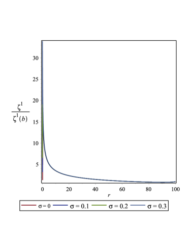
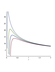
Figure 5: Radial components of geodesic deviation for Kiselev BH surrounded by radiation with IC$1$ for different values radiation parameter with $M=1$, $q=0.6$ and $b=100$.

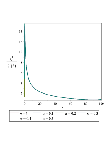
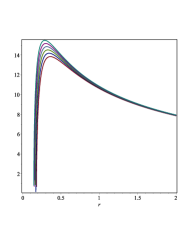
Figure 6: Radial components of geodesic deviation for Kiselev BH surrounded by dust with IC$1$ for different values dust parameter with $M=1$, $q=0.6$ and $b=100$.

Here, $\zeta^{\hat{1}}(b)$ and $\zeta^{\hat{i}}(b)$ are the radial and angular components of the initial geodesic deviation vector at $r=b$ and $\dot{\zeta}^{\hat{1}}(b)$ and $\dot{\zeta}^{\hat{i}}(b)$ are the corresponding derivatives with respect to the proper time $\tau$. Figure 5-10 represents the radial and angular components of the geodesic deviation vector of a body in-falling from rest at $r=b$ towards BH for different choices of the radiation and dust parameters. We choose the initial condition (IC$1$) $\zeta^{\hat{1}}(b)>0$, $\dot{\zeta}^{\hat{1}}(b)=0$ and $\zeta^{\hat{i}}(b)>0$, $\dot{\zeta}^{\hat{i}}(b)=0$. It represents the releasing a body at rest consisting of dust with no internal motion. On the other hand, we choose the initial condition (IC$2$) $\zeta^{\hat{1}}(b)=0$, $\dot{\zeta}^{\hat{1}}(b)>0$ and $\zeta^{\hat{i}}(b)=0$, $\dot{\zeta}^{\hat{i}}(b)>0$. It corresponds to letting such a body explode from a point at $r=b$. The behavior of the geodesic deviation vector is almost identical for different values of radiation and dust parameter until r becomes of the same order as the horizon radius.

In Figure 5, the radial tidal force for Kiselev BH surrounded by radiation depends upon the radiation parameter with IC$1$ i.e. it attains the highest maximum value at $\sigma_{r}=0.3$ while as the radiation parameter decrease the maximum value of radial tidal force also decreases. Also the maximum value is shifting towards BH as the radiation parameter increases. For $\sigma_{r}>0.3$, it becomes unphysical. Figure 6 represents the radial tidal force for Kiselev BH surrounded by dust for different choices of dust parameter with IC$1$. It is clear from figure the maximum value of radial tidal force is increasing as the value of dust parameter increases as well as it shifting towards the BH. It is concluded that the maxima of radial tidal force depends upon radiation and dust parameter, it increases for large values of $\sigma_{r}$ and $\sigma_{d}$. Figures 7 and 8 represent the radial tidal forces for Kiselev BH surrounded by radiation and dust parameter for its different choices with IC$2$. In Figure 7, maxima of radial tidal force is increasing for higher values of radiation parameter and attains the maximum value at $\sigma_{r}=0.3$, and also it is shifted towards the BH as the radiation parameter increases. But in Figure 8, maximum value of radial tidal force is same for all chosen values of dust parameter. Although, the radial tidal force is shifting towards the BH as the dust parameter increases.

The angular tidal force for Kiselev BH surrounded by radiation and dust parameter with IC$1$ is similar as explained in [26], as it does not depend upon radiation and dust parameter. However, the angular tidal force with IC$2$ are discussed in Figure 9 and 10 for Kiselev BH surrounded by radiation and dust respectively. It can be seen in Figure 9 that the angular tidal force is increasing from $r=100$ and attains maximum value at $r=50$ then start decreasing, reflecting the compressing nature of angular component. At some point near the BH, angular tidal force start increasing as shown in Figure 9. Also, it is shifting towards the singularity as radiation parameter increases. In Figure 10, the angular tidal force have the maximum value for $\sigma_{d}=0$, while it decreases for large values of dust parameter.

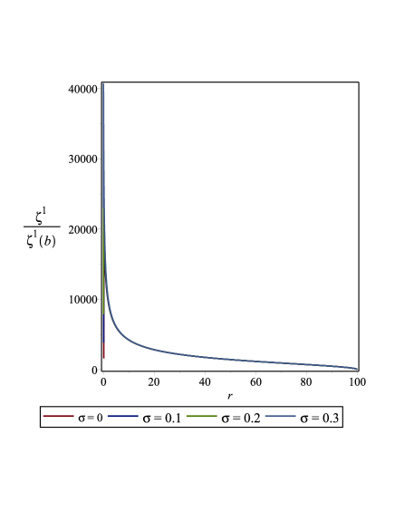
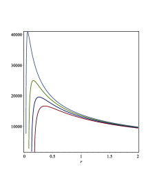
Figure 7: Radial components of geodesic deviation for Kiselev BH surrounded by radiation with IC$2$ for different values radiation parameter with $M=1$, $q=0.6$ and $b=100$.

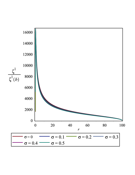
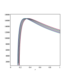
Figure 8: Radial components of geodesic deviation for Kiselev BH surrounded by dust with IC$2$ for different values dust parameter with $M=1$, $q=0.6$ and $b=100$.

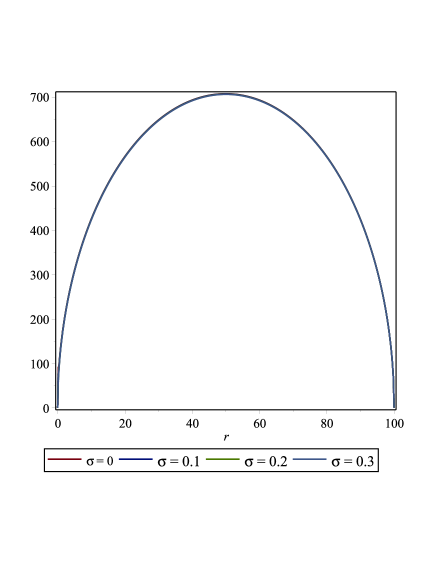
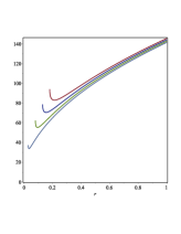
Figure 9: Angular components of geodesic deviation for Kiselev BH surrounded by radiation with IC$2$ for different values radiation parameter with $M=1$, $q=0.6$ and $b=100$.

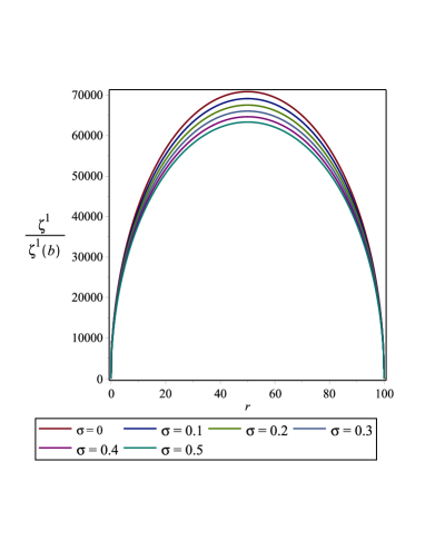
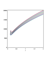
Figure 10: Angular components of geodesic deviation for Kiselev BH surrounded by dust with IC$2$ for different values dust parameter with $M=1$, $q=0.6$ and $b=100$.

$\sigma_{d}$	$r_{+}$	$rtf$	$atf$	$Figure~{}6$	$Figure~{}8$	$Figure~{}10$
0	1.8	0.2400	-0.1371	8.2543	9935.44	19160.04
0.1	1.9116	0.2197	-.1233	8.0509	9455.87	19221.57
0.2	2.0219	0.2015	-.1115	7.8615	9020.038	19271.458
0.3	2.1310	0.1852	-.1013	7.6845	8622.22	19312.18
0.4	2.2392	0.1707	-0.0925	7.5186	8257.65	19345.57
0.5	2.3465	0.1578	-0.0848	7.3627	7922.33	19373.02

Table 1: Location of event horizon for chosen values of dust parameter.

$\sigma_{d}$	$r_{-}$	$rtf$	$atf$	$Figure~{}6$	$Figure~{}8$	$Figure~{}10$
0	0.2	-425.00	100.00	8.2542	9935.44	8343.08
0.1	0.1883	-544.31	129.03	8.0508	9455.87	7966.709
0.2	0.1780	-684.94	163.34	7.8615	9020.03	7625.47
0.3	0.1689	-849.08	203.51	7.6845	8622.22	7314.24
0.4	0.1607	-1039.06	250.10	7.5186	8257.65	7028.92
0.5	0.1534	-1257.28	303.70	7.3627	7922.33	6766.19

Table 2: Location of Cauchy horizon for chosen values of dust parameter.

$\sigma_{r}$	$r_{+}$	$rtf$	$atf$	$Figure~{}5$	$Figure~{}7$	$Figure~{}9$
0	1.8	0.24	-.1371	8.2542	9935.44	191.60
0.1	1.8602	0.2455	-.1336	8.2522	9925.43	193.59
0.2	1.9165	0.2485	-.1302	8.2501	9915.44	195.40
0.3	1.9695	0.2498	-.1269	8.2480	9905.47	197.05

Table 3: Location of event horizon for chosen values of radiation parameter.

$\sigma_{r}$	$r_{-}$	$rtf$	$atf$	$Figure~{}5$	$Figure~{}7$	$Figure~{}9$
0	0.2	-425.00	100.00	8.2542	9935.44	83.4308
0.1	.1397	-1311.44	315.06	8.2521	9925.43	71.5674
0.2	0.08348	-6443.99	1575.13	8.2500	9915.44	57.0569
0.3	0.0304	-138248.39	34292.71	8.2479	9905.47	36.0236

Table 4: Location of Cauchy horizon for chosen values of radiation parameter.

Table 1 - 4 represent the location of event horizon and Cauchy horizon for chosen values of radiation and dust parameter. Here, we find the location of event and Cauchy horizons of rtf (Figures 1 and 2), atf (Figures 3 and 4), radial tidal force with IC$1$ (Figures 5, 6) and IC$2$ (Figures 7, 8), respectively and angular tidal force with IC$2$ (Figures 9 and 10) for chosen values of radiation and dust parameter, respectively. It is noted that the radial tidal force (in Figures 1 and 2) and angular tidal force (in Figures 3 and 4) change their sign between event and Cauchy horizons. Event horizon is increasing (away from singularity) and Cauchy horizon is decreasing (shifting towards singularity) as the radiation and dust parameter increase.

5 Conclusion

We investigated the tidal forces of Kiselev BHs by assuming its two special cases, i.e. Kiselev BH surrounded by radiation and dust. We have observed that the radial tidal forces can change its behavior from stretching to compressing for specific choices of radiation and dust parameters and angular tidal forces can only be zero between event and Cauchy horizons of BH. It is also mention here that the radial and angular tidal forces possesses an ability to change their sign between event and Cauchy horizons. Event horizon is increasing (away from singularity) and Cauchy horizon is decreasing (shifting towards singularity) as the radiation and dust parameter increase. Furthermore, the geodesic deviation equations can be solved analytically about radially free-falling geodesic for Kiselev BH [26]. The behavior of geodesic deviation vector for such a geodesic under the influence of tidal forces are examined. We choose the initial condition IC$1$ which represents the releasing a body at rest consisting of dust with no internal motion and IC$2$ corresponds to letting such a body explode from a point at $r=b$. It is pointed out here that the radial tidal forces for Kiselev BH surrounded by radiation attains the maximum value at $\sigma_{r}=0.3$ as shown in Figure 5 and it becomes unphysical for $\sigma_{r}>0.3$. Moreover, the maxima of radial tidal forces for Kiselev BH surrounded by dust is increasing as well as shifting towards the BH as the dust parameter increasing. These are the agreement with [26]. Hence it is concluded that the radial component of geodesic deviation vector becomes zero while angular component remain finite for certain initial condition.

References

- [1] Perlmutter, S., et al.: Supernova Cosmology Project Collaboration. Astrophys. J. 517, 565 (1999).
- [2] Spergel, D.N., et al.: WMAP Collaboration. Astrophys. J. Suppl. 170, 377 (2007).
- [3] Eisenstein, D.J. et al.: SDSS Collaboration. Astrophys. J. 633, 560 (2005).
- [4] Riess, A.G. et al.: Supernova Search Team Collaboration. Astron. J. 116, 1009 (1998).
- [5] Johri, V.B.: Phys. Rev. D 70, 041303 (2004).
- [6] Lobo, F.S.N.: Phys. Rev. D 71, 084011 (2005).
- [7] D Inverno, R.: Introducing Einstein s Relativity (Clarendon Press, Oxford, 1992).
- [8] Hobson, M.P., Efstathiou, G., Lasenby, A.N.: General Relativity An Introduction for Physicists (Cambridge University Press, Cambridge, 2006).
- [9] Schutz, B.F.: A First Course in General Relativity (Cambridge University Press, Cambridge, 1985).
- [10] Misner, C.W., Thorne, K.S., Wheeler, J.A.: Gravitation(W.H.Freeman and Co., New York, 1973).
- [11] Hartle, J.B.: Gravity: An Introduction to Einstein s General Relativity (Addison-Wesley, San Francisco, 2002).
- [12] Abdel-Megied, Gad, R.M.: Chaos Solitons Fractals 23, 313 (2005).
- [13] Chandrasekhar, S.: The Mathematical Theory of Black Holes (Clarendon Press, Oxford, 1983).
- [14] Misner, C., Thorne, K., Wheeler, J.: Gravitation. Freeman, San Francisco (1973).
- [15] Adler, R., Bazin, M., Schiffer, M.: Introduction to General Relativity, 2nd edn. McGraw-Hill, New York (1975).
- [16] Ghosh, S., Kar, S.: arXiv:0904.2321v1 [gr-qc] (2009).
- [17] Bekenstein, J.D.: Ann. Phys. 91, 75 (1975).
- [18] Ayon-Beato, E., Garcia, A.: Gen. Relat. Grav. 31, 629 (1999).
- [19] Garfinkle, D., Horowitz, G.T., Strominger, A.: Phys. Rev. D 43, 3140 (1991).
- [20] Garfinkle, D., Horowitz, G.T., Strominger, A.: Phys. Rev. D 45, 3888(E) (1992).
- [21] Jawad, A. and Shahzad, M.U.: Eur. Phys. J. C 76, 123 (2016).
- [22] Kiselev, V. V.: Class. Quant. Grav. 20, 1187 (2003).
- [23] Yang, R. J.: arXiv:1605.02320 (2016).
- [24] Younas, A., et al.: Phys. Rev. D 92, 084042 (2015).
- [25] Majeed, B., Jamil, M., Pradhan, P.: Advances in High Energy Physics 2015, 124910, (2015).
- [26] Crispino, L.C.B., et al.: Eur. Phys. J. C 76, 168 (2016).
- [27] Penrose, R.: in Singularities and Time Asymmetry, in General Relativity, an Einstein Centenary Survey, ed. by S.W. Hawking, W. Israel, (Cambridge University Press, Cambridge, 1979)
- [28] Wald, R.M.: General Relativity (The University of Chicago Press, Chicago, 1984).
- [29] Martel, K., Poisson, E. : Phys. Rev. D 66, 084001 (2002).
- [30] Symon, K.R.: Mechanics (Addison-Wesley Publishing Company, Massachusetts, 1971).