Metropolis-Hastings reversiblizations of non-reversible Markov chains

Abstract.

We study two types of Metropolis-Hastings (MH) reversiblizations for non-reversible Markov chains with Markov kernel $P$. While the first type is the classical Metropolised version of $P$, we introduce a new self-adjoint kernel which captures the opposite transition effect of the first type, that we call the second MH kernel. We investigate the spectral relationship between $P$ and the two MH kernels. Along the way, we state a version of Weyl’s inequality for the spectral gap of $P$ (and hence its additive reversiblization), as well as an expansion of $P$. Both results are expressed in terms of the spectrum of the two MH kernels. In the spirit of Fill (1991) and Paulin (2015), we define a new pseudo-spectral gap based on the two MH kernels, and show that the total variation distance from stationarity can be bounded by this gap. We give variance bounds of the Markov chain in terms of the proposed gap, and offer spectral bounds in metastability and Cheeger’s inequality in terms of the two MH kernels by comparison of Dirichlet form and Peskun ordering.

AMS 2010 subject classifications: Primary 60J05, 60J10; Secondary 60J20, 37A25, 37A30

Keywords: non-reversible Markov chain; spectral gap; Metropolis-Hastings algorithm; mixing time; Weyl’s inequality; variance bounds

1. Introduction

Consider a Markov chain with Markov kernel $P$ and stationary distribution $\pi$ with its time-reversal $P^{*}$ on a general state space $\mathcal{X}$. The quantitative rate of convergence to equilibrium is well-known to be closely connected to the spectrum or the spectral gap of $P$, see for instance Aldous and Fill (2002); Saloff-Coste (1997); Levin et al. (2009); Montenegro and Tetali (2006); Meyn and Tweedie (2009) and the references therein. In the reversible case, that is, when $P$ is viewed as a linear self-adjoint operator in $L^{2}(\pi)$, Roberts and Rosenthal (1997) shows that the existence of an $L^{2}$-spectral gap is equivalent to $P$ being geometrically ergodic. The main technical insight relies heavily on the spectral theory of self-adjoint operators, which facilitates the analysis of the spectrum of $P$.

However, $P$ need not be reversible in general. If $P$ is non-reversible, the analysis on the rate of convergence is fragmentally understood, possibly due to a much less developed spectral theory for non-self-adjoint operators. We now describe three different approaches that have been elaborated to overcome this difficulty.

The first approach, initiated by Fill (1991), is to resort to an appropriate reversiblized version of $P$ and analyze how its spectrum can be related to the chi-squared distance to stationarity of the original chain. Two reversiblizations are proposed, namely the multiplicative reversiblization $PP^{*}$ and the additive reversiblization $(P+P^{*})/2$. In the discrete-time setting, it is shown that the second largest eigenvalue of $PP^{*}$ can be used to upper bound the distance from stationarity, while the spectral gap of $(P+P^{*})/2$ is used for continuous-time Markov chain. More recently, Paulin (2015) generalizes this approach and defines a pseudo-spectral gap, based upon the maximum spectral gap of $P^{*k}P^{k}$ for $k\geqslant 1$. He demonstrates that the proposed gap plays a similar role as that of spectral gap in the reversible case. He proves variance bounds and Bernstein inequality based on his proposed gap. In this vein, we also mention the work of Jerison (2013) who gives mixing time bounds for general non-reversible Markov chains in terms of absolute spectral gap.

The second approach, proposed by Kontoyiannis and Meyn (2012), is to cast $P$ in a weighted Banach space $L^{\infty}_{V}$ instead of the classical $L^{2}(\pi)$ framework, where $V$ is a Lyapunov function associated with $P$. In particular, they show that for a $\phi$-irreducible and aperiodic Markov chain, $P$ is geometrically ergodic if and only if $P$ admits a spectral gap in the space $L^{\infty}_{V}$ equipped with the $V$-norm. They also give an example in which a non-reversible Markov chain is geometrically ergodic yet it fails to have a $L^{2}(\pi)$ spectral gap.

The third approach, initiated by Patie and Savov (2018) and Miclo (2016), is to resort to intertwining relationship, to build a link between the non-reversible and reversible chains. Patie and Savov (2018) investigated the rate of convergence to equilibrium of the generalized Laguerre semigroup and the hypocoercivity phenomenon. Recently, by means of the concept of similarity, Choi and Patie (2019) investigated the rate of convergence to equilibrium of skip-free chains and the cut-off phenomenon.

The path taken in this paper is in the spirit of the first approach and stems on an additional reversiblization procedure. More specifically, we use and develop further the celebrated Metropolis-Hastings (MH) algorithm to provide an original in-depth analysis of non-reversible chains. The aim is to investigate Metropolis-Hastings (MH) reversiblizations, and how it helps to analyze non-reversible chains. The MH algorithm, developed by Metropolis et al. (1953) and Hastings (1970), is a Markov Chain Monte Carlo method that is of fundamental importance in statistics and other applications, see e.g. Roberts and Rosenthal (2004) and the references therein. The idea is to construct from a proposal kernel a reversible chain which converges to a desired distribution. Much of the literature focuses on the speed of convergence of specific algorithms, where the proposal kernel (e.g. a random walk proposal or an Ornstein-Uhlenbeck proposal) is often by itself reversible and the target density is in general not the proposal stationary measure. For example, Roberts and Tweedie (1996) investigates the random walk MH with exponential family target density. Hairer et al. (2014) compares the theoretical performance of random walk MH and pCN algorithm with target density given by their equation $1.1,1.2$ by establishing their Wasserstein spectral gap.

The notion of MH reversiblizations to study non-reversible chains is not entirely new. To the best of our knowledge, this term is first formally introduced by Aldous and Fill (2002), although they did not provide a detailed analysis. Our contributions can be summarized as follows:

1. We start by studying two types of MH reversiblizations. The first MH kernel is the classical Metropolis chain of $P$, and we identify a new self-adjoint yet possibly non-Markovian operator that we call the second MH kernel. It captures the opposite transition effect of the first kernel, and thus it can be interpreted as the dual in a broad sense. We show that the linear operator $P+P^{*}$ can be written as the sum of the two MH kernels, which allows us to state a version of Weyl’s inequality for the spectral gap of $P$ and its additive reversiblization in the finite state space case. We prove that our bound is sharp by investigating in detail the asymmetric simple random walk on the $n$-cycle. We also give a spectral-type expansion of $P$ expressed in terms of the spectral measures of the two MH kernels, which we call a MH pseudospectral expansion, in terms of the spectral measures of the two MH kernels.

2. We proceed by defining a pseudo-spectral gap, that we call the MH-spectral gap, based on the spectrum of the two MH kernels, along the line of work by Paulin (2015). We show that the existence of a MH-spectral gap implies that $P$ is geometrically ergodic. We carry out some numerical examples that reveal that our MH-spectral gap is, for non-reversible chains, a better estimate than the existing bounds found in the literature. Variance bounds are also proved in terms of the proposed gap. Finally, we revisit the notion of metastability and the Cheeger’s inequality, to offer a variant of these celebrated inequalities by means of comparison of the non-reversible chain and the two MH kernels.

The rest of the paper is organized as follows. We fix the notation and give a review of the theory of general state space Markov chains as well as the MH algorithm in Section 2. We begin Section 3 by formally defining the two MH kernels and state some elementary results, followed by comparing $P$ and the two MH kernels using the Peskun ordering, and we end this section by stating Weyl’s inequality for the spectral gap of $P$. Section 4 describes the pseudospectral expansion of $P$. The MH-spectral gap is defined in Section 5, and we give a number of results that relate Weyl’s inequality, geometric ergodicity, mixing time and the MH-spectral gap. Finally, we state the results about variance bounds in terms of the MH-spectral gap in Section 6, and discuss metastability and the Cheeger’s inequality bounds in Section 7.

2. Preliminaries

In this section, we review several fundamental notions for Markov chains on a general state space.

Let $X=(X_{n})_{n\in\mathbb{N}_{0}}$ be a time-homogeneous Markov chain on a measurable state space $(\mathcal{X},\mathcal{F})$, and as usual we write $P$ to be the Markov kernel which describes the one-step transition. Recall that for $P:\mathcal{X}\times\mathcal{F}\to[0,1]$ to be a Markov kernel, for each fixed $A\in\mathcal{F}$, the mapping $x\mapsto P(x,A)$ is $\mathcal{F}$-measurable and for each fixed $x\in\mathcal{X}$, the function $A\mapsto P(x,A)$ is a probability measure on $\mathcal{X}$. As we need to handle possibly non-Markovian general kernels in the sequel, we say that a general kernel $K$ acts on a given function $f:\mathcal{X}\to\mathbb{C}$ from the left and a signed measure $\mu$ on $(\mathcal{X},\mathcal{F})$ from the right by

$$Kf(x):=\int_{\mathcal{X}}f(y)K(x,dy),\quad\mu K(A):=\int_{\mathcal{X}}K(x,A)\mu(dx),\quad x\in\mathcal{X},A\in\mathcal{F},$$

whenever the integrals exist.

We say that $\pi$ is a stationary distribution of $X$ if $\pi$ is a probability measure on $(\mathcal{X},\mathcal{F})$ and

$$\int_{\mathcal{X}}P(x,A)\,\pi(dx)=\pi(A),\quad A\in\mathcal{F}.$$

A closely related notion is reversibility. We say that $X$ is reversible if there is a probability measure $\pi$ on $(\mathcal{X},\mathcal{F})$ such that the detailed balance relation is satisfied:

$$\pi(dx)P(x,dy)=\pi(dy)P(y,dx).$$

Note that detailed balance means the two probability measures are identical on the product space $(\mathcal{X}\times\mathcal{X},\mathcal{F}\times\mathcal{F})$. It is known that if $\pi$ is a reversible probability measure, then $\pi$ is a stationary distribution, yet the converse is not true. Let $L^{2}(\pi)$ be the Hilbert space of complex valued measurable functions on $\mathcal{X}$ that are squared-integrable with respect to $\pi$, endowed with the inner product $\langle f,g\rangle_{\pi}:=\int f\overline{g}\,d\pi$ and the norm $||f||_{\pi}:=\langle f,f\rangle_{\pi}^{1/2}$, where the overline $\overline{g}$ is the complex conjugate of $g$. $P$ can then be viewed as a linear operator on $L^{2}(\pi)$, in which we still denote the operator by $P$. The operator norm of $P$ on $L^{2}(\pi)$ is

$$||P||_{L^{2}\to L^{2}}=\sup_{\begin{subarray}{c}f\in L^{2}(\pi)\\ ||f||_{\pi}=1\end{subarray}}||Pf||_{\pi}.$$

Let $P^{*}$ be the adjoint or time-reversal of $P$ on $L^{2}(\pi)$, and it can be checked that

$$\pi(dx)P^{*}(x,dy)=\pi(dy)P(y,dx).$$

This shows that reversibility is equivalent to self-adjointness of $P$. Write $\sigma(P)=\sigma(P|L^{2})$ to be the spectrum of $P$ on $L^{2}(\pi)$, i.e.

$$\sigma(P|L^{2})=\{\lambda\in\mathbb{C}\backslash 0:(\lambda I-P)\,\text{does not have a bounded inverse}\}.$$

If $P$ is self-adjoint, then $\sigma(P)\subseteq[-1,1]$. In addition, the spectral theorem for self-adjoint operators gives

(2.1) $$P=\int_{\sigma(P)}\lambda\,\mathcal{E}(d\lambda),$$

where $\mathcal{E}$ is the spectral measure associated with $P$. When considering the spectral gap of $P$, it is often convenient for us to restrict to the space $L^{2}_{0}(\pi)=\{f\in L^{2}(\pi):\mathbb{E}_{\pi}f=0\}$. We formally define the meaning of an $L^{2}$-spectral gap.

Definition 2.1 ($L^{2}$-spectral gap).

Suppose that $P$ is a Markov kernel with stationary measure $\pi$. If

$$\beta=||P||_{L^{2}_{0}\to L^{2}_{0}}<1,$$

then the (absolute) $L^{2}$-spectral gap is $\gamma^{*}=\gamma^{*}(P)=1-\beta$.

Let

$$\lambda=\lambda(P):=\inf\{\alpha:\alpha\in\sigma(P|L^{2}_{0})\},\quad\Lambda=\Lambda(P):=\sup\{\alpha:\alpha\in\sigma(P|L^{2}_{0})\}.$$

If $P$ is reversible with respect to $\pi$, then it is known that (see, e.g. Rudolf (2012))

(2.2) $$\lambda=\inf_{\begin{subarray}{c}f\in L^{2}_{0}(\pi)\\ ||f||_{\pi}=1\end{subarray}}\langle Pf,f\rangle_{\pi},\quad\Lambda=\sup_{\begin{subarray}{c}f\in L^{2}_{0}(\pi)\\ ||f||_{\pi}=1\end{subarray}}\langle Pf,f\rangle_{\pi},$$

$$||P||_{L^{2}_{0}\to L^{2}_{0}}=\sup_{\begin{subarray}{c}f\in L^{2}_{0}(\pi)\\ ||f||_{\pi}=1\end{subarray}}|\langle Pf,f\rangle_{\pi}|.$$

This allows us to deduce that

(2.3) $$\beta=\max\{|\lambda|,\Lambda\}.$$

We also define the (right) spectral gap for a Markov kernel.

Definition 2.2 (spectral gap).

Suppose that $P$ is a Markov kernel with stationary measure $\pi$. The (right) spectral gap is defined to be

$$\gamma=\gamma(P):=1-\sup\{\mathrm{Re}(\alpha):\alpha\in\sigma(P|L^{2}_{0})\}.$$

If $P$ is reversible, then $\gamma=1-\Lambda(P)$. In the finite state space setting, it can be shown that $\gamma(P)=\gamma((P+P^{*})/2)$ (see e.g. (Saloff-Coste, 1997, discussion after Definition $2.1.3$, where we can consider $\lambda$ therein to be our $\gamma(P)$)), so for a general $P$ on a finite state space,

$$\gamma(P)=1-\Lambda((P+P^{*})/2).$$

Remark 2.1.

We recall that in Fill (1991), additive reversiblization $(P+P^{*})/2$ and multiplicative reversiblization $PP^{*}$ are proposed to study mixing for non-reversible chains. In the discrete-time setting, the upper bound involves $\gamma(PP^{*})$, while for continuous-time Markov chains, the upper bound depends on $\gamma((P+P^{*})/2)$.

Remark 2.2.

In Paulin (2015), a pseudo-spectral gap based on the spectral gap of $P^{*k}P^{k}$ for $k\geqslant 1$ is introduced. Precisely, we define

$$\gamma^{ps}=\gamma^{ps}(P):=\max_{k\geqslant 1}\{\gamma(P^{*k}P^{k})/k\}.$$

2.1. The Metropolis-Hastings kernel

Let $\pi$ be a probability measure on $(\mathcal{X},\mathcal{F})$ that is absolutely continuous with density $\pi$ (with a slight abuse of notation, the density is still denoted by $\pi$) with respect to a reference measure $\mu$ on $\mathcal{X}$, that is, $\pi(dx)=\pi(x)\mu(dx)$. Denote $Q$ to be any Markov kernel on $\mathcal{X}$, where $Q(x,\cdot)$ is absolutely continuous with density $q$ with respect to $\mu$. $\pi$ is the so-called target distribution, while $Q$ is commonly known as the proposal kernel. Define the acceptance probabilities $\alpha(x,y)$ by

$$\alpha(x,y)=\begin{cases}\min\left(\dfrac{\pi(y)q(y,x)}{\pi(x)q(x,y)},1\right)&\mbox{if }\pi(x)q(x,y)>0,\\ 0&\mbox{otherwise.}\end{cases}$$

Let $p(x,y):=\alpha(x,y)q(x,y)$, and define the reject probabilities $r:\mathcal{X}\to[0,1]$ via $r(x):=1-\int p(x,y)\mu(dy)$. The Metropolis-Hastings kernel $P$ is given by

$$P(x,dy)=p(x,y)\mu(dy)+r(x)\delta_{x}(dy),$$

where $\delta_{x}$ is the point mass at $x$.

The MH kernel allows for the following algorithmic interpretation. First, we choose $X_{0}$ and given the current state $X_{n}$, we generate the proposal $Y_{n+1}$ by $Q(X_{n},\cdot)$. With probability $\alpha(X_{n},Y_{n+1})$, we accept the proposal and set $X_{n+1}=Y_{n+1}$. Otherwise, we reject $Y_{n+1}$ and set $X_{n+1}=X_{n}$. Finally, we set $n=n+1$ and the above procedure is repeated.

Markov Chain Monte Carlo (MCMC) methods, such as the classical Metropolis-Hastings algorithm, involve constructing a Markov chain which converges to a desired stationary distribution $\pi$ that one would like to sample from. It differs from Monte Carlo methods in the sense that $\pi$ is often difficult to simulate directly, and is particularly useful in situations where we only know $\pi$ up to normalization constants. As described in Roberts and Rosenthal (2004), we can see that the choice of the proposal kernel $Q$ has an significant impact on the performance of the MH algorithm. Common choices of $Q$ includes the symmetric MH ($q(x,y)=q(y,x)$), random walk MH ($q(x,y)=q(y-x)$) and independence MH ($q(x,y)=q(y)$).

3. Metropolis-Hastings reversiblizations

From now on, unless otherwise stated, we assume $X$ is a $\phi$-irreducible Markov chain, which may not be reversible, with Markov kernel $P$ and stationary distribution $\pi$. We also assume that $P(x,\cdot)$, $P^{*}(x,\cdot)$ and $\pi$ share a common dominating reference measure $\mu$ on $(\mathcal{X},\mathcal{F})$, with density denoted by $p(x,\cdot)$, $p^{*}(x,\cdot)$ and $\pi(\cdot)$, respectively. Furthermore, we assume that the set $\{x:\pi(x)=0\}$ is a $\mu$-null set.

Given a Markov chain $X$ with Markov kernel $P$ and stationary distribution $\pi$, we can obtain a MH-reversiblized chain by taking the proposal kernel to be $P$. The resulting process is what we called the first MH chain.

Definition 3.1 (The first MH kernel).

The first MH chain, with Markov kernel denoted by $M_{1}:=M_{1}(P)$, is the MH kernel with proposal kernel $P$ and target distribution $\pi$. That is, let

$$\alpha_{1}(x,y) =\begin{cases}\min\left(\dfrac{\pi(y)p(y,x)}{\pi(x)p(x,y)},1\right)&\mbox{if }\pi(x)p(x,y)>0,\\ 0&\mbox{otherwise,}\end{cases}$$

$$m_{1}(x,y) =\alpha_{1}(x,y)p(x,y)=\min\{p^{*}(x,y),p(x,y)\},$$

$$r_{1}(x) =\int_{y\neq x}(1-\alpha_{1}(x,y))p(x,y)\,\mu(dy),$$

then $M_{1}$ is given by

$$M_{1}(x,dy)=m_{1}(x,y)\mu(dy)+r_{1}(x)\delta_{x}(dy).$$

By taking a closer look at $m_{1}$, we can see that the first MH chain weakens the transition to $A_{x}:=\{y\in\mathcal{X}:\alpha_{1}(x,y)<1\}$, and follows the same transition as the original chain $X$ for $A_{x}^{c}=\{y:\alpha_{1}(x,y)=1\}$. This motivates us to develop what we call the second MH kernel $M_{2}:=M_{2}(P)$ with density $m_{2}$, which captures the opposite transition of $M_{1}$. Precisely, we would like to have

$$m_{2}(x,y)=\begin{cases}p(x,y)&\mbox{if }y\in A_{x},\\ p^{*}(x,y)&\mbox{if }y\in A_{x}^{c}\backslash\{x\}.\end{cases}=\max\{p^{*}(x,y),p(x,y)\}.$$

As a result, we obtain the following:

Definition 3.2 (The second MH kernel).

The second MH kernel $M_{2}:=M_{2}(P)$ and density $m_{2}$ are given by

$$m_{2}(x,y) =\max\{p^{*}(x,y),p(x,y)\},$$

$$M_{2}(x,dy) =m_{2}(x,y)\mu(dy)-r_{1}(x)\delta_{x}(dy).$$

Note that $M_{2}$ in general may not be a Markov kernel, since there is no guarantee that $M_{2}(x,\{x\})=P(x,\{x\})-r_{1}(x)\geqslant 0$. For instance, if $P$ is the Markov kernel of a finite Markov chain with $P(x,x)=0$ for all $x\in\mathcal{X}$, then $M_{2}(x,x)=-r_{1}(x)\leqslant 0$. In the following we collect a few elementary properties of $M_{1}$ and $M_{2}$.

Lemma 3.1.

Suppose that $P$ is a Markov kernel with stationary measure $\pi$, with $M_{1}$ and $M_{2}$ being the first and second MH kernel of $P$ respectively. Then the following holds.

1. $P+P^{*}=M_{1}+M_{2}$. In particular, $M_{2}(x,\mathcal{X})=1$, for $x\in\mathcal{X}$.

2. $M_{1}$ and $M_{2}$ are self-adjoint operators on $L^{2}(\pi)$.

3. $M_{1}=M_{2}=P$ if and only if $P$ is reversible with respect to $\pi$.

4. $M_{i}(P)=M_{i}(P^{*})$ for $i=1,2$.

[Proof. ]

1. This can easily be seen from Definition 3.1 and 3.2 together with

   $$p(x,y)+p^{*}(x,y)=\min\{p^{*}(x,y),p(x,y)\}+\max\{p^{*}(x,y),p(x,y)\}.$$

2. It is well known that $M_{1}$ is reversible (and hence invariant) w.r.t. $\pi$, see e.g. (Roberts and Rosenthal, 2004, Proposition $2$). To see that $M_{2}$ is a self-adjoint operator on $L^{2}(\pi)$, we use (i). That is,

   $$M_{2}^{*}=(P+P^{*}-M_{1})^{*}=P^{*}+P-M_{1}=M_{2}.$$

3. If $M_{1}=M_{2}=P$, then (i) gives $P^{*}=M_{1}+M_{2}-P=P$. Conversely, when $P$ is reversible w.r.t. $\pi$, then $\alpha(x,y)=1$ $\mu\times\mu\,a.e.$, and hence $M_{1}=P$ by Definition 3.1. It follows again from (i) that $M_{2}=P+P^{*}-M_{1}=P$.

4. Using the fact that $P^{**}=P$ and Definition 3.1, $M_{1}(P)=M_{1}(P^{*}).$ Next, (i) gives

   $$M_{2}(P)=P+P^{*}-M_{1}(P)=P^{*}+P-M_{1}(P^{*})=M_{2}(P^{*}).$$

Remark 3.1.

As remarked earlier, although $M_{2}$ is not a Markov kernel in general, it is a self-adjoint operator in $L^{2}(\pi)$ and satisfies $\pi M_{2}=\pi(P+P^{*}-M_{1})=\pi$.

3.1. Peskun Ordering

We aim to investigate some further relationships and properties of the spectra of $P,M_{1}$ and $M_{2}$ via the so-called Peskun ordering, which was first introduced by Peskun (1973) as a partial ordering for Markov kernels on finite state space, and was further generalized by Tierney (1998) to general state space.

Definition 3.3 (Peskun Ordering).

Suppose that $P_{1},P_{2}$ are general kernels with invariant distribution $\pi$. $P_{1}$ dominates $P_{2}$ off the diagonal, written as $P_{1}\succeq P_{2}$, if for $\pi$-almost all $x$, $P_{1}(x,A)\geqslant P_{2}(x,A)$ for all $A\in\mathcal{F}$ with $x\notin A$.

Note that we are not restricting to Markov kernels in Definition 3.3, since $M_{2}$ in general may not be a Markov kernel. Even in this setting, we can still demonstrate that the results obtained by Tierney (1998) hold in the following lemma:

Lemma 3.2.

Suppose that $P$ is a Markov kernel with stationary measure $\pi$, with $M_{1}$ and $M_{2}$ being the first and second MH kernel of $P$ respectively. We have the following:

1. $M_{2}\succeq P\succeq M_{1}$.

2. $P-M_{2}$, $M_{1}-P$ and $M_{1}-M_{2}$ are positive semidefinite operators.

[Proof. ]

1. For $x\in\mathcal{X}$ and $A\in\mathcal{F}$ with $x\notin A$,

   $$M_{2}(x,A)=\int_{A}\max\{p(x,y),p^{*}(x,y)\}\mu(dy)\geqslant P(x,A)\geqslant\int_{A}\min\{p(x,y),p^{*}(x,y)\}\mu(dy)=M_{1}(x,A).$$

2. We modify the proof of Lemma $3$ in Tierney (1998) to cater for the case where $M_{2}$ may not be a Markov kernel. Let $H(dx,dy)=\pi(dx)(\delta_{x}(dy)-P(x,dy)+M_{2}(x,dy))$. Lemma 3.1 yields $H(A)\geqslant 0$ , $H(\mathcal{X}\times\mathcal{X})=1$, $H(\mathcal{X}\times B)=H(B\times\mathcal{X})=\pi(B)$ for $A\in\mathcal{F}\otimes\mathcal{F}$ and $B\in\mathcal{F}$. The rest of the proof are the same as the proof of Lemma $3$ in Tierney (1998).

Corollary 3.1.

Suppose that $P$ is a Markov kernel with stationary measure $\pi$, with $M_{1}$ and $M_{2}$ being the first and second MH kernel of $P$ respectively. Using the notation defined in (2.2), we obtain:

(3.1) $$\lambda(M_{2})\leqslant\inf_{\begin{subarray}{c}f\in L^{2}_{0}(\pi)\\ ||f||_{\pi}=1\end{subarray}}\langle Pf,f\rangle_{\pi}\leqslant\lambda(M_{1}),$$

(3.2) $$\Lambda(M_{2})\leqslant\sup_{\begin{subarray}{c}f\in L^{2}_{0}(\pi)\\ ||f||_{\pi}=1\end{subarray}}\langle Pf,f\rangle_{\pi}\leqslant\Lambda(M_{1}).$$

[Proof. ]Lemma 3.2 leads to

$$\langle M_{2}f,f\rangle_{\pi}\leqslant\langle Pf,f\rangle_{\pi}\leqslant\langle M_{1}f,f\rangle_{\pi}.$$

Desired result follows by taking infimum or supremum over $\{f\in L^{2}_{0}(\pi):||f||_{\pi}=1\}$, (2.2) and Lemma 3.1(i).

Inspired by Corollary 3.1 and (2.3), we will introduce a pseudo-spectral gap (that we will call the MH-spectral gap) based on $\lambda(M_{2})$ and $\Lambda(M_{1})$ in Section 5. We will obtain a number of new bounds based on this gap.

3.2. Weyl’s inequality for additive reversiblization

In this section, we introduce Weyl’s inequality for the additive reversiblization for finite Markov chains, which allows us to give upper and lower bound on the eigenvalues of $(P+P^{*})/2$, in terms of the eigenvalues of $M_{1}(P)$ and $M_{2}(P)$. Assume that $P$ is a stochastic matrix on a finite state space $\mathcal{X}$ with stationary distribution $\pi$, with eigenvalues-eigenvectors denoted by $(\lambda_{j}(P),\phi_{j}(P))_{j=1}^{|\mathcal{X}|}$. If $P$ is a self-adjoint matrix, we arrange its eigenvalues in non-increasing order by $\lambda_{1}(P)\geqslant\ldots\geqslant\lambda_{n}(P)$, where $n:=|\mathcal{X}|$. We write $l^{2}(\pi)$ to be the Hilbert space of square-summable function with respect to $\pi$.

Theorem 3.1 (Weyl’s inequality for additive reversiblization).

Assume that $P$ is a $n\times n$ stochastic matrix with stationary distribution $\pi$, with $M_{1}$, $M_{2}$ to be the first and second MH kernel.

1. For integers $i,j,k$ such that $1\leqslant i,j,k\leqslant n$ and $i+1=j+k$,

   $$\lambda_{i}(P+P^{*})\leqslant\lambda_{j}(M_{1})+\lambda_{k}(M_{2}).$$

   Equality holds if and only if there exists a vector $f$ with $||f||_{l^{2}(\pi)}=1$ such that $M_{1}f=\lambda_{j}f,M_{2}f=\lambda_{k}f$ and $(P+P^{*})f=\lambda_{i}f$.

2. For integers $i,l,m$ such that $1\leqslant i,l,m\leqslant n$ and $i+n=l+m$,

   $$\lambda_{i}(P+P^{*})\geqslant\lambda_{l}(M_{1})+\lambda_{m}(M_{2}).$$

   Equality holds if and only if there exists a vector $f$ with $||f||_{l^{2}(\pi)}=1$ such that $M_{1}f=\lambda_{l}f,M_{2}f=\lambda_{m}f$ and $(P+P^{*})f=\lambda_{i}f$.

[Proof. ]Thanks to Lemma 3.1(i), $P+P^{*}=M_{1}+M_{2}$, where both $M_{1}$ and $M_{2}$ are self-adjoint matrices in $l^{2}(\pi)$. Desired results follow directly from Weyl’s inequality, see e.g. Theorem $4.3.1$ in Horn and Johnson (2013).

Since $\gamma(P)=\gamma((P+P^{*})/2)$, we can obtain bounds on the spectral gap of $P$ in terms of the eigenvalues of $M_{1},M_{2}$.

Corollary 3.2.

With the assumptions of Theorem 3.1, we have

$$1-\dfrac{1}{2}U\leqslant\gamma(P)\leqslant 1-\dfrac{1}{2}L,$$

where $L:=\max_{l+m=2+n}\{\lambda_{l}(M_{1})+\lambda_{m}(M_{2})\}$ and $U:=\min_{j+k=3}\{\lambda_{j}(M_{1})+\lambda_{k}(M_{2})\}$.

[Proof. ]We take $i=2$ in Theorem 3.1 to obtain

$$\dfrac{1}{2}L\leqslant\lambda_{2}((P+P^{*})/2)\leqslant\dfrac{1}{2}U.$$

Desired result follows by using $\gamma(P)=\gamma((P+P^{*})/2)=1-\lambda_{2}((P+P^{*})/2)$.

3.3. Examples: asymmetric random walk and birth-death processes with vortices

In this section, we first show that the bounds in Corollary 3.2 are sharp by studying the asymmetric simple random walk on $n$-cycle and on discrete torus. We then proceed to give spectral gap bounds for birth-death processes with vortices.

Example 3.1 (Asymmetric simple random walk on the $n$-cycle).

We first recall the asymmetric simple random walk on the $n$-cycle. We take $\mathcal{X}=\{0,1,\ldots,n-1\}$ and the transition matrix to be $P(j,k)=p$ for $k=j+1\mod{n}$, $P(j,k)=q=1-p$ for $k=j-1\mod{n}$ and $0$ otherwise. Its stationary distribution is given by $\pi(i)=1/n$ for all $i\in\mathcal{X}$, and its time-reversal has transition matrix given by $P^{*}=P^{T}$, the transpose of $P$. In the particular case when $p=q=1/2$, we recover the symmetric random walk with eigenvalues $(\cos(2\pi j/n))_{j=0}^{n-1}$, which have been studied in Levin et al. (2009); Fill (1991); Diaconis and Stroock (1991).

We denote $l:=\min\{p,q\}$ and $r:=\max\{p,q\}$. Then $M_{1}$ and $M_{2}$ are given by, for $j\in\mathcal{X}$,

$$M_{1}(j,k) =l,\quad\mathrm{for}\,k=j\pm 1\mod{n},\quad M_{1}(j,j)=1-2l,$$

$$M_{2}(j,k) =r,\quad\mathrm{for}\,k=j\pm 1\mod{n},\quad M_{2}(j,j)=1-2r.$$

Note that $M_{2}$ is not a Markov kernel unless $r=p=q=1/2$. For $p\neq 1/2$, we can interpret $M_{2}$ as $M_{2}=G+I$, where $G:=M_{2}-I$ is the Markov generator on $\mathcal{X}$. Using the notation of Section 3.2 and observe that the additive reversiblization is the simple symmetric random walk, the unordered eigenvalues of $(P+P^{*})/2$, $M_{1}$ and $M_{2}$ (see Example $3.1,3.2$ in Fill (1991)) are, for $i\in\{1,\ldots,n\}$,

$$\lambda_{i}((P+P^{*})/2) =\cos(2\pi(i-1)/n),$$

$$\lambda_{i}(M_{1}) =1-2l(1-\cos(2\pi(i-1)/n)),$$

$$\lambda_{i}(M_{2}) =1-2r(1-\cos(2\pi(i-1)/n)),$$

so Corollary 3.2 now reads $L=2\cos(2\pi/n)$, $U=2-2r(1-\cos(2\pi/n))$ and

$$r(1-\cos(2\pi/n))=1-\dfrac{1}{2}U\leqslant\gamma(P)=1-\cos(2\pi/n)=1-\dfrac{1}{2}L,$$

that is, the upper bound is exactly attained and the lower bound is sharp in $n$.

Example 3.2 (Asymmetric simple random walk on discrete torus).

This example investigates the asymmetric simple random walk on discrete torus $\mathbb{Z}_{n}^{d}=(\mathbb{Z}\backslash n\mathbb{Z})^{d}$, in which we build a product chain via the asymmetric kernel on the $n$-cycle that we studied in Example 3.1 and we also adapt the notations therein. That is, we choose one of the $d$ coordinates at random and it will move according to the kernel $P(j,k)=p$ for $k=j+1\mod{n}$, $P(j,k)=q=1-p$ for $k=j-1\mod{n}$ and $0$ otherwise. Denote the Markov kernel (resp. first Metropolis kernel, second Metropolis kernel) on $\mathbb{Z}_{n}^{d}$ by $\widetilde{P}$ (resp. $\widetilde{M_{1}}$, $\widetilde{M_{2}}$), then we have

$$\widetilde{P} =\dfrac{1}{d}\sum_{i=1}^{d}\underbrace{I\otimes\cdots\otimes I}_{i-1}\otimes P\otimes\underbrace{I\otimes\cdots\otimes I}_{d-i},$$

$$\widetilde{M_{1}} =\dfrac{1}{d}\sum_{i=1}^{d}\underbrace{I\otimes\cdots\otimes I}_{i-1}\otimes M_{1}\otimes\underbrace{I\otimes\cdots\otimes I}_{d-i},$$

$$\widetilde{M_{2}} =\dfrac{1}{d}\sum_{i=1}^{d}\underbrace{I\otimes\cdots\otimes I}_{i-1}\otimes M_{2}\otimes\underbrace{I\otimes\cdots\otimes I}_{d-i}.$$

Note that the stationary distribution is the uniform distribution on $\mathbb{Z}_{n}^{d}$. The unordered eigenvalues of $(\widetilde{P}+\widetilde{P}^{*})/2$, $\widetilde{M_{1}}$ and $\widetilde{M_{2}}$ are, for $i\in\{1,\ldots,n\}$,

$$\lambda_{i}((\widetilde{P}+\widetilde{P}^{*})/2) =(d-1)/d+\cos(2\pi(i-1)/n)/d,$$

$$\lambda_{i}(\widetilde{M_{1}}) =1-2l(1-\cos(2\pi(i-1)/n))/d,$$

$$\lambda_{i}(\widetilde{M_{2}}) =1-2r(1-\cos(2\pi(i-1)/n))/d.$$

and Corollary 3.2 now reads $L=2-2/d+2\cos(2\pi/n)/d$, $U=2-2r(1-\cos(2\pi/n))/d$ and

$$r(1-\cos(2\pi/n))/d=1-\dfrac{1}{2}U\leqslant\gamma(P)=\dfrac{1-\cos(2\pi/n)}{d}=1-\dfrac{1}{2}L,$$

that is, the upper bound is exactly attained and the lower bound is sharp in $n$.

Example 3.3 (Inserting vortices to birth-death processes).

Giving two-sided precise spectral gap bounds for non-reversible Markov chains is well-known to be a difficult task. For the spectral gap estimates of birth-death processes, we refer interested readers to Chen (1996). We aim at using this example to show how we can give such type of estimates by means of MH reversibilization. This example is inspired by Sun et al. (2010); Bierkens (2016), which offers an interesting way to artificially create non-reversible Markov chains from reversible ones via perturbation or inserting vortices. It is perhaps more suitable to work in the setting of continuous-time Markov chains. We write $G^{BD}$ to be the infinitesimal generator of a birth-death process with birth rate $b_{i}$ and death rate $d_{i}$ for $i\in\mathcal{X}=\mathbb{N}_{0}$ with stationary distribution $\pi(i)$. Next, we denote $V$ to be the $n$-dimensional cyclic vortices given by $V(i,i)=-1/\pi(i)$ and $V(i,j)=1/\pi(i)$ for $j=(i+1)\mod{n}$ for $i\in\{0,\ldots,n\}$. By Corollary $1$ in Sun et al. (2010), $G:=G^{BD}+V$ is the generator of a non-reversible Markov chain on $\mathcal{X}$ with stationary distribution $\pi$.

To analyze the left spectral gap $\gamma(G)$ of $-G$, the construction of $M_{1}$ and $M_{2}$ applies essentially in verbatim to $G$ as in Section 3. More precisely, we define $\gamma(G)$ to be the smallest distance between the spectrum of $-G$ to $0$, i.e.

$$\gamma(G):=-\sup_{\begin{subarray}{c}f\in L^{2}_{0}(\pi)\\ ||f||_{\pi}=1\end{subarray}}\langle Gf,f\rangle_{\pi}=\gamma((G+G^{*})/2),$$

where we used $\langle Gf,f\rangle_{\pi}=\langle((G+G^{*})/2)f,f\rangle_{\pi}$ in the equality above. Note that the Peskun ordering of generator gives

$$\langle M_{2}(G)f,f\rangle_{\pi}\leqslant\langle Gf,f\rangle_{\pi}\leqslant\langle M_{1}(G)f,f\rangle_{\pi}.$$

Specializing the above into our examples of birth-death processes with vortices, we take $G^{*}=G^{BD}+V^{*}$, $M_{1}(G)=G^{BD}$ and $M_{2}(G)=G^{BD}+V+V^{*}$. As a result, it follows that

$$\gamma(G^{BD})\leqslant\gamma(G)\leqslant\gamma(G^{BD})+\gamma(V+V^{*})\leqslant\gamma(G^{BD})+\dfrac{2}{\min_{i\in\{0,\ldots,n\}}\pi(i)}(1-\cos(2\pi/n)),$$

where we further upper bound the left spectral gap of $V+V^{*}$ by the symmetric random walk on $n$-cycle with birth and death rate $1/\min_{i\in\{0,\ldots,n\}}\pi(i)$. We can then specialize into various well-known examples of birth-death processes, in which we summarize the results below:

Process	spectral gap bounds
Ehrenfest with vortices	$1\leqslant\gamma(G)\leqslant 1+2(1-\cos(2\pi/n))\max\{p^{-n},(1-p)^{-n}\}$
$M/M/1$ with vortices	$(\sqrt{\mu}-\sqrt{\lambda})^{2}\leqslant\gamma(G)\leqslant(\sqrt{\mu}-\sqrt{\lambda})^{2}+2(1-\lambda/\mu)^{-1}(\mu/\lambda)^{n-1}(1-\cos(2\pi/n))$
$M/M/\infty$ with vortices	$1\leqslant\gamma(G)\leqslant 1+2(1-\cos(2\pi/n))e^{\lambda}\max_{i\in\{0,\ldots,n\}}i!\lambda^{-i}$
GWI with vortices	$1-\lambda\leqslant\gamma(G)\leqslant 1-\lambda+2(1-\cos(2\pi/n))\max_{i\in\{0,\ldots,n\}}\dfrac{\Gamma(r)i!}{\Gamma(r+i)}(1-\lambda)^{-r}\lambda^{-i}$

Table 1. Spectral gap bounds for various birth-death processes with $n$-dimensional cyclic vortices

For the Ehrenfest model with cyclic vortices, it is constructed from a birth-death process with $b_{i}=p(n-i)$, $d_{i}=(1-p)i$ with $0<p<1$ on $\mathcal{X}=\{0,\ldots,n\}$ and $\pi$ being the binomial distribution with parameters $n$ and $p$. For $M/M/1$ with vortices, it is constructed from a birth-death process with $b_{i}=\lambda$, $d_{i}=\mu$ with $\mu>\lambda$ and $\pi(i)=(1-\lambda/\mu)(\lambda/\mu)^{i-1}$. For $M/M/\infty$ with vortices, it is constructed from a birth-death process with $b_{i}=\lambda$, $d_{i}=i$ and $\pi$ being the Poisson distribution with mean $\lambda$. For the Galton-Watson process with immigration (GWI) and vortices, we have $b_{i}=\lambda(r+i)$, $d_{i}=i$ and $\pi$ being the negative binomial distribution with parameters $\lambda$ and $r$.

In the literature, the reciprocal of $\gamma(G)$ is commonly known as the relaxation time, which serves as a lower bound in the total variation mixing time of the chain, see for instance (Jerison, 2013, Theorem $1$). This means that the reciprocal of the upper bound of the spectral gap in the table above can be used to give lower bound on the total variation mixing time. In Section 5, we formally introduce various notions of ergodicity of Markov chain as well as total variation mixing time. In this spirit, we would like to mention the work of (Fill, 1991, Section $4$) and Chen (1996). In the former, the author studied upper and lower bounds of the spectral gaps of exclusion processes, while in the latter the author investigated two-sided spectral gap bounds of classical birth-death processes.

4. Pseudospectral expansion

As a consequence of Lemma 3.1(ii), $M_{1}$ and $M_{2}$ are self-adjoint operators on $L^{2}(\pi)$, which help us to obtain a pseudospectral expansion of $P$ in terms of the spectral measures of $M_{1}$ and $M_{2}$.

Theorem 4.1.

Denote $P$ to be a Markov kernel with stationary distribution $\pi$, and $M_{i}$ to be the MH kernel (defined in def. 3.1 and def. 3.2) with spectral measure $\mathcal{E}_{i}$ for $i=1,2$. For $x\in\mathcal{X}$, $B\in\mathcal{F}$ with $x\notin B$, we have

(4.1) $$P(x,B) =\int_{\sigma(M_{1})}\lambda\,\delta_{x}\mathcal{E}_{1}(d\lambda)(B\cap A_{x}^{c})+\int_{\sigma(M_{2})}\lambda\,\delta_{x}\mathcal{E}_{2}(d\lambda)(B\cap A_{x}),$$

(4.2) $$P(x,\{x\}) =\dfrac{1}{2}\left(\int_{\sigma(M_{1})}\lambda\,\delta_{x}\mathcal{E}_{1}(d\lambda)(\{x\})+\int_{\sigma(M_{2})}\lambda\,\delta_{x}\mathcal{E}_{2}(d\lambda)(\{x\})\right),$$

(4.3) $$P^{*}(x,B) =\int_{\sigma(M_{1})}\lambda\,\delta_{x}\mathcal{E}_{1}(d\lambda)(B\cap A_{x})+\int_{\sigma(M_{2})}\lambda\,\delta_{x}\mathcal{E}_{2}(d\lambda)(B\cap A_{x}^{c}),$$

where we recall that $A_{x}:=\{y\in E:\alpha_{1}(x,y)<1\}$.

[Proof. ]We first show (4.1). By Lemma 3.1 and (2.1), for $i=1,2$,

(4.4) $$M_{i} =\int_{\sigma(M_{i})}\lambda\,\mathcal{E}_{i}(d\lambda).$$

Therefore, we can deduce that

$$P(x,B) =P(x,B\cap A_{x}^{c})+P(x,B\cap A_{x})$$

$$=\int_{B\cap A_{x}^{c}}P(x,dy)+\int_{B\cap A_{x}}P(x,dy)$$

$$=\int_{B\cap A_{x}^{c}}M_{1}(x,dy)+\int_{B\cap A_{x}}M_{2}(x,dy)\quad(\mathds{1}_{B}(x)=0)$$

$$=\delta_{x}M_{1}(B\cap A_{x}^{c})+\delta_{x}M_{2}(B\cap A_{x})$$

$$=\int_{\sigma(M_{1})}\lambda\,\delta_{x}\mathcal{E}_{1}(d\lambda)(B\cap A_{x}^{c})+\int_{\sigma(M_{2})}\lambda\,\delta_{x}\mathcal{E}_{2}(d\lambda)(B\cap A_{x}).\quad\text{(By \eqref{eq:Mispecthm})}$$

Next, in view of Lemma 3.1, we have

$$P(x,\{x\}) =\dfrac{1}{2}\left(M_{1}(x,\{x\})+M_{2}(x,\{x\})\right)$$

$$=\dfrac{1}{2}\left(\int_{\sigma(M_{1})}\lambda\,\delta_{x}\mathcal{E}_{1}(d\lambda)(\{x\})+\int_{\sigma(M_{2})}\lambda\,\delta_{x}\mathcal{E}_{2}(d\lambda)(\{x\})\right),$$

which gives (4.2). Finally, to show (4.3), we follow a very similar proof of (4.1) that leads to

$$P^{*}(x,B) =P^{*}(x,B\cap A_{x})+P^{*}(x,B\cap A_{x}^{c})$$

$$=\delta_{x}M_{1}(B\cap A_{x})+\delta_{x}M_{2}(B\cap A_{x}^{c})$$

$$=\int_{\sigma(M_{1})}\lambda\,\delta_{x}\mathcal{E}_{1}(d\lambda)(B\cap A_{x})+\int_{\sigma(M_{2})}\lambda\,\delta_{x}\mathcal{E}_{2}(d\lambda)(B\cap A_{x}^{c}).$$

Remark 4.1.

When $P$ is reversible, Lemma 3.1 yields $P=M_{1}=M_{2}$, so (4.1) and (4.2) reduces to

$$P(x,B) =\int_{\sigma(P)}\lambda\,\delta_{x}\mathcal{E}_{1}(d\lambda)(B),$$

$$P(x,\{x\}) =\int_{\sigma(P)}\lambda\,\delta_{x}\mathcal{E}_{1}(d\lambda)(\{x\}),$$

which are expected expressions (since we can invoke the spectral theorem directly on $P$).

Remark 4.2.

An alternative expression for $P(x,\{x\})$ is the following: Using (4.1) (with $B$ replaced by $\mathcal{X}\backslash\{x\}$), we observe that

$$P(x,\{x\}) =1-P(x,\mathcal{X}\backslash\{x\})$$

$$=1-\int_{\sigma(M_{1})}\lambda\,\delta_{x}\mathcal{E}_{1}(d\lambda)(\mathcal{X}\backslash\{x\}\cap A_{x}^{c})-\int_{\sigma(M_{2})}\lambda\,\delta_{x}\mathcal{E}_{2}(d\lambda)(\mathcal{X}\backslash\{x\}\cap A_{x})$$

$$=\int_{\sigma(M_{1})}\lambda\,\delta_{x}\mathcal{E}_{1}(d\lambda)(\{x\}\cup A_{x})-\int_{\sigma(M_{2})}\lambda\,\delta_{x}\mathcal{E}_{2}(d\lambda)(A_{x}).$$

To compute the pseudospectral expansion of the $n$-step Markov kernel $P^{n}$, we can make use of the Chapman-Kolmogorov equation together with (4.1) and (4.2). Equivalently, we can replace $P$ by $P^{n}$ in Theorem 4.1, which leads to:

Corollary 4.1.

Denote $P$ to be a Markov kernel with stationary measure $\pi$, so that $P^{n}$ is the n-step Markov kernel for $n\in\mathbb{N}$. Let $M_{i}(P^{n})$ to be the MH kernel (defined in def. 3.1 and def. 3.2) with spectral measure $\mathcal{E}_{i}(P^{n})$ for $i=1,2$. For $x\in\mathcal{X}$, $B\in\mathcal{F}$ with $x\notin B$, we have

(4.5) $$P^{n}(x,B) =\int_{\sigma(M_{1}(P^{n}))}\lambda\,\delta_{x}\mathcal{E}_{1}(P^{n})(d\lambda)(B\cap A_{x}^{c})+\int_{\sigma(M_{2}(P^{n}))}\lambda\,\delta_{x}\mathcal{E}_{2}(P^{n})(d\lambda)(B\cap A_{x}),$$

(4.6) $$P^{n}(x,\{x\}) =\dfrac{1}{2}\left(\int_{\sigma(M_{1}(P^{n}))}\lambda\,\delta_{x}\mathcal{E}_{1}(P^{n})(d\lambda)(\{x\})+\int_{\sigma(M_{2}(P^{n}))}\lambda\,\delta_{x}\mathcal{E}_{2}(P^{n})(d\lambda)(\{x\})\right),$$

(4.7) $$P^{*n}(x,B) =\int_{\sigma(M_{1}(P^{n}))}\lambda\,\delta_{x}\mathcal{E}_{1}(P^{n})(d\lambda)(B\cap A_{x})+\int_{\sigma(M_{2}(P^{n}))}\lambda\,\delta_{x}\mathcal{E}_{2}(P^{n})(d\lambda)(B\cap A_{x}^{c}),$$

where $A_{x}:=\{y:\alpha_{1}(P^{n})(x,y)<1\}$.

Next, we specialize into the case of finite Markov chains, as more explicit results can be obtained.

Corollary 4.2.

Suppose that $P$ is a Markov kernel on a finite state space $\mathcal{X}$ with stationary distribution $\pi$. Let $M_{i}(P^{n})$ be the MH kernel with eigenvalues-eigenvectors denoted by $(\lambda^{(i)}_{j},\phi^{(i)}_{j})_{j=1}^{|\mathcal{X}|}$ for $i=1,2$ (note that the dependence of $(\lambda^{(i)}_{j},\phi^{(i)}_{j})$ on $P^{n}$ is suppressed). For $x\in\mathcal{X}$ and $f\in l^{2}(\pi)$, we have

(4.8) $$P^{n}(x,y) =\begin{cases}\sum_{j=1}^{|\mathcal{X}|}\lambda^{(2)}_{j}\phi^{(2)}_{j}(x)\phi^{(2)}_{j}(y)\pi(y)&\mbox{if }y\in A_{x},\\ \sum_{j=1}^{|\mathcal{X}|}\lambda^{(1)}_{j}\phi^{(1)}_{j}(x)\phi^{(1)}_{j}(y)\pi(y)&\mbox{if }y\in A_{x}^{c}\backslash\{x\},\\ \dfrac{1}{2}(\sum_{j=1}^{|\mathcal{X}|}\lambda^{(1)}_{j}\phi^{(1)}_{j}(x)\phi^{(1)}_{j}(x)\pi(x)+\sum_{j=1}^{|\mathcal{X}|}\lambda^{(2)}_{j}\phi^{(2)}_{j}(x)\phi^{(2)}_{j}(x)\pi(x))&\mbox{if }y=x.\end{cases}$$

(4.9) $$P^{n}f(x) =\sum_{j=1}^{|\mathcal{X}|}\lambda^{(1)}_{j}\phi^{(1)}_{j}(x)\langle f\mathds{1}_{A_{x}^{c}\backslash\{x\}},\phi^{(1)}_{j}\rangle_{\pi}+\sum_{j=1}^{|\mathcal{X}|}\lambda^{(2)}_{j}\phi^{(2)}_{j}(x)\langle f\mathds{1}_{A_{x}},\phi^{(2)}_{j}\rangle_{\pi}+P^{n}(x,x)f(x),$$

where $A_{x}:=\{y:\alpha_{1}(P^{n})(x,y)<1\}$.

[Proof. ]The proof of (4.8) follows from (4.5) and (4.6). To see (4.9), we decompose $P^{n}f(x)$ into

$$P^{n}f(x) =P^{n}f\mathds{1}_{A_{x}^{c}\backslash\{x\}}(x)+P^{n}f\mathds{1}_{A_{x}}(x)+P^{n}f\mathds{1}_{\{x\}}(x)$$

(4.10) $$=M_{1}(P^{n})f\mathds{1}_{A_{x}^{c}\backslash\{x\}}(x)+M_{2}(P^{n})f\mathds{1}_{A_{x}}(x)+P^{n}f\mathds{1}_{\{x\}}(x).$$

Now, since $(\phi^{(i)}_{j})_{j=1}^{|\mathcal{X}|}$ is a basis on $l^{2}(\pi)$ for $i=1,2$, we have

(4.11) $$M_{1}(P^{n})f\mathds{1}_{A_{x}^{c}\backslash\{x\}}(x) =\sum_{j=1}^{|\mathcal{X}|}\lambda^{(1)}_{j}\phi^{(1)}_{j}(x)\langle f\mathds{1}_{A_{x}^{c}\backslash\{x\}},\phi^{(1)}_{j}\rangle_{\pi},$$

(4.12) $$M_{2}(P^{n})f\mathds{1}_{A_{x}}(x) =\sum_{j=1}^{|\mathcal{X}|}\lambda^{(2)}_{j}\phi^{(2)}_{j}(x)\langle f\mathds{1}_{A_{x}},\phi^{2}_{j}\rangle_{\pi}.$$

Desired result follows by collecting (4.10), (4.11) and (4.12).

5. Geometric ergodicity, mixing time and MH-spectral gap

We will measure the speed of convergence to stationarity by the total variation distance, which is defined to be:

Definition 5.1 (Total variation distance).

The total variation distance between two signed measures $\mu$ and $\nu$ is given by

$$||\mu-\nu||_{TV}:=\sup_{A}|\mu(A)-\nu(A)|=\dfrac{1}{2}\sup_{|f|\leqslant 1}|\mu(f)-\nu(f)|.$$

where $|f|:=\sup_{x\in\mathcal{X}}|f(x)|$.

We refer the readers to Levin et al. (2009), Meyn and Tweedie (2009) and Roberts and Rosenthal (2004) for further properties of the total variation distance. In our main results in Section 5.1 below, we are primarily interested in the case when $\mu$ is either $P(x,\cdot)$, $P^{*}(x,\cdot)$, $M_{1}(x,\cdot)$ or $M_{2}(x,\cdot)$ for $x\in\mathcal{X}$, while $\nu$ is taken to be the stationary measure $\pi$. We can now define various notions of ergodicity of a general kernel $K$.

Definition 5.2 (Geometric ergodic, $\pi$-a.e. geometrically ergodic, uniformly ergodic, mixing time).

Suppose that $K$ is a general kernel with stationary measure $\pi$, that is, $\pi K=\pi$. $K$ is geometrically ergodic if for each probability measure $\mu$, there exists $C_{\mu}<\infty$ and $\rho\in[0,1)$ such that

(5.1) $$||\mu K^{n}-\pi||_{TV}\leqslant C_{\mu}\rho^{n},\quad n\in\mathbb{N}.$$

If (5.1) holds with $\mu=\delta_{x}$ for $\pi$-a.e. $x$, then $K$ is called $\pi$-a.e. geometrically ergodic. $K$ is uniformly ergodic if there exists $C<\infty$ and $\rho\in[0,1)$ such that

(5.2) $$d(n):=\sup_{x\in\mathcal{X}}||K^{n}(x,\cdot)-\pi||_{TV}\leqslant C\rho^{n},\quad n\in\mathbb{N}.$$

The mixing time $t_{mix}(\epsilon)$ is defined to be

$$t_{mix}(\epsilon):=\min\{n:d(n)\leqslant\epsilon\}.$$

Similar to the remarks after Definition 5.1 above, in subsequent sections we consider the case when the kernel $K$ is taken to be either $P,P^{*},M_{1}$ or $M_{2}$. In particular, it is because of $M_{2}$ that we introduce these general notions of ergodicity for non-Markovian kernels. For Markov kernels that are reversible w.r.t. $\pi$, we have the following characterization of geometric ergodicity in terms of the $L^{2}$-spectral gap.

Theorem 5.1.

Suppose that $P$ is reversible with respect to $\pi$. The following statements are equivalent:

1. $P$ is geometrically ergodic.

2. $P$ admits a $L^{2}$-spectral gap, i.e. $\gamma^{*}=1-\beta=1-\max\{|\lambda|,\Lambda\}>0.$

The proof can be found in Roberts and Rosenthal (1997).

5.1. Main results

Following from the result in Corollary 3.1 and (2.3), we can define a pseudo-spectral gap by taking $1-\max\{|\lambda(M_{2})|,\Lambda(M_{1})\}$. However, this gap may not be informative as $|\lambda(M_{2})|$ maybe greater than or equal to $1$ since $M_{2}$ is not a Markov kernel in general. To define a meaningful gap, we should consider $M_{2}$ with $|\lambda(M_{2})|<1$. This leads us to the following definition:

Definition 5.3 (MH-spectral gap).

Suppose that $P$ is a Markov kernel with stationary measure $\pi$. Let

$$\mathcal{C} :=\{n\in\mathbb{N}:|\lambda(M_{2}(P^{n}))|<1,\Lambda(M_{1}(P^{n}))<1\},\quad\mathcal{C}^{c}:=\mathbb{N}\backslash\mathcal{C},$$

$$\beta^{MH} :=\begin{cases}1,&\text{if $\mathcal{C}=\emptyset$,}\\ \sup_{n\in\mathcal{C}}\{|\lambda(M_{2}(P^{n}))|^{1/n},\Lambda(M_{1}(P^{n}))^{1/n}\},&\text{otherwise.}\end{cases}$$

The MH-spectral gap $\gamma^{MH}=\gamma^{MH}(P)$ is given by

$$\gamma^{MH}:=1-\beta^{MH}.$$

In this definition, we insert the idea of “burn-in" in MCMC to define a MH-spectral gap. Precisely, we discard the spectral gaps in $\mathcal{C}^{c}$, and only consider the gaps in $\mathcal{C}$.

Note that for reversible $P$, the $L^{2}$-spectral gap is equal to the MH-spectral gap. If $P$ is geometrically ergodic, Lemma 3.1(iii) and Theorem 5.1 lead to $\mathcal{C}=\mathbb{N}$ and

$$\gamma^{MH} =1-\beta^{MH}$$

$$=1-\sup_{n\in\mathbb{N}}\{|\lambda(P^{n})|^{1/n},\Lambda(P^{n})^{1/n}\}$$

$$=1-\sup_{n\in\mathbb{N}}\{|\lambda(P)|,\Lambda(P)\}$$

$$=1-\max\{|\lambda(P)|,\Lambda(P)\}=1-\beta=\gamma^{*}.$$

If $P$ is not geometrically ergodic, then $\beta^{MH}=\beta=1$, so $\gamma^{MH}=\gamma^{*}=0$.

As a first result, by means of Weyl’s inequality, we can show that $M_{2}=M_{2}(P)$ is a contraction whenever $P$ is a finite-state lazy and ergodic Markov kernel. Recall that a finite-state Markov chain is said to be lazy if $p(x,x)\geqslant 1/2$, and ergodic if $P$ is irreducible and aperiodic.

Theorem 5.2.

If $P$ is a finite-state lazy and ergodic Markov kernel, then $|\lambda(M_{2}(P))|\leqslant 1$.

[Proof. ]By Weyl’s inequality introduced in Theorem 3.1, we have

$$\lambda_{n}(P+P^{*})\leqslant\lambda_{1}(M_{1})+\lambda_{n}(M_{2})=1+\lambda_{n}(M_{2}).$$

Note that laziness of $P$ implies the laziness of $(P+P^{*})/2$, which implies $0\leqslant\lambda_{n}(P+P^{*})\leqslant 1+\lambda_{n}(M_{2})$. On the other hand, using Corollary 3.1 and the fact that $M_{1}$ is a Markov kernel, we have $\lambda_{n}(M_{2})\leqslant\lambda_{n}(M_{1})\leqslant 1$.

Next, we present the main results in this section. Theorem 5.3 shows that a MH-spectral gap leads to geometric ergodicity.

Theorem 5.3.

Suppose that $P$ is the Markov kernel of a $\phi$-irreducible and aperiodic Markov chain with stationary measure $\pi$ on a countably generated state space $\mathcal{X}$. If $|\mathcal{C}^{c}|<\infty$ and $P$ admits a MH-spectral gap, i.e. $\gamma^{MH}=1-\beta^{MH}>0$, then $P$ and $P^{*}$ are geometrically ergodic (and $\pi$-a.e. geometrically ergodic).

Next, we demonstrate a partial converse to Theorem 5.3.

Theorem 5.4.

[Partial converse of Theorem 5.3] Suppose that $P$ is a Markov kernel with stationary measure $\pi$. If $P$ and $P^{*}$ are uniformly ergodic, then there exists a $N\in\mathbb{N}$ such that for all $n\geqslant N$, $M_{i}(P^{n})$ are uniformly ergodic for $i=1,2$.

Recall that in the reversible case Theorem 5.1 gives the existence of $L^{2}$-spectral gap is equivalent to geometric ergodicity. While we hope for a result that characterizes geometric ergodicity in the non-reversible case by means of the MH-spectral gap, we only manage to show that under a stronger assumption of uniform ergodicity of both $P$ and $P^{*}$, $M_{i}(P^{n})$ is uniformly ergodic for sufficiently large $n$. This implies the existence of an $L^{2}$-spectral gap of $M_{i}(P^{n})$ for sufficiently large $n$, yet it is unclear whether $\beta^{MH}$ is less than $1$ (since we are taking supremum in the definition of $\beta^{MH}$).

Next, we present a result that gives a mixing time upper bound in terms of the MH-spectral gap.

Corollary 5.1.

For a finite Markov chain with Markov kernel $P$ that is irreducible, if $|\mathcal{C}^{c}|<\infty$ and $P$ admits a MH-spectral gap, then

$$t_{mix}(\epsilon)\leqslant t^{*}+\dfrac{\log\left(\frac{1}{\epsilon\pi_{min}}\right)}{\gamma^{MH}},$$

where $t^{*}:=\max_{n\in\mathcal{C}^{c}}n$ and $\pi_{min}:=\min_{x}\pi(x)$.

Corollary 5.1 can be compared with the result in the reversible case (Theorem $12.3$ in Levin et al. (2009)), which shows that

$$t_{mix}(\epsilon)\leqslant\dfrac{\log\left(\frac{1}{\epsilon\pi_{min}}\right)}{\gamma^{*}}.$$

This also follows from Corollary 5.1 since $|\mathcal{C}^{c}|=0$ and $\gamma^{MH}=\gamma^{*}$ in the reversible case.

5.2. Proofs of Theorem 5.3, Theorem 5.4 and Corollary 5.1

First, we start with the following result that allows us to control the total variation distance of $P^{n}$ and $P^{*n}$ to $\pi$ by means of that of $M_{1}(P^{n})$ and $M_{2}(P^{n})$ and vice versa. The bounds are by no means tight, yet they will serve their purpose to demonstrate geometric ergodicity in the proof of Theorem 5.3 and Theorem 5.4.

Lemma 5.1.

Suppose that $P$ is a Markov kernel with stationary measure $\pi$, and $M_{i}$ to be the MH kernel for $i=1,2$. For $x\in\mathcal{X}$, $n\in\mathbb{N}$,

$$||P^{n}(x,\cdot)-\pi||_{TV} \leqslant\dfrac{3}{2}||M_{1}(P^{n})(x,\cdot)-\pi||_{TV}+\dfrac{3}{2}||M_{2}(P^{n})(x,\cdot)-\pi||_{TV},$$

$$||P^{*n}(x,\cdot)-\pi||_{TV} \leqslant\dfrac{3}{2}||M_{1}(P^{n})(x,\cdot)-\pi||_{TV}+\dfrac{3}{2}||M_{2}(P^{n})(x,\cdot)-\pi||_{TV},$$

$$||M_{1}(P^{n})(x,\cdot)-\pi||_{TV} \leqslant 2||P^{n}(x,\cdot)-\pi||_{TV}+2||P^{*n}(x,\cdot)-\pi||_{TV},$$

$$||M_{2}(P^{n})(x,\cdot)-\pi||_{TV} \leqslant 3||P^{n}(x,\cdot)-\pi||_{TV}+3||P^{*n}(x,\cdot)-\pi||_{TV}.$$

[Proof. ]We use the same idea as in the proof of Theorem 4.1. For any $x\in E$ let $A_{x,n}:=\{y:\alpha_{1}(P^{n})(x,y)<1\}$. We have, for all $n\in\mathbb{N}$,

$$||P^{n}(x,\cdot)-\pi||_{TV} =\sup_{A}|P^{n}(x,A)-\pi(A)|$$

$$\leqslant\sup_{A}|P^{n}(x,A\cap A_{x,n})-\pi(A\cap A_{x,n})|+\sup_{A}|P^{n}(x,A\cap A_{x,n}^{c}\backslash\{x\})-\pi(A\cap A_{x,n}^{c}\backslash\{x\})|$$

$$\quad+|P^{n}(x,\{x\})-\pi(\{x\})|$$

$$\leqslant||M_{2}(P^{n})(x,\cdot)-\pi||_{TV}+||M_{1}(P^{n})(x,\cdot)-\pi||_{TV}+\dfrac{1}{2}|M_{1}(P^{n})(x,\{x\})-\pi(\{x\})|$$

$$\quad+\dfrac{1}{2}|M_{2}(P^{n})(x,\{x\})-\pi(\{x\})|$$

$$\leqslant\dfrac{3}{2}||M_{1}(P^{n})(x,\cdot)-\pi||_{TV}+\dfrac{3}{2}||M_{2}(P^{n})(x,\cdot)-\pi||_{TV}.$$

To show the inequality for $||P^{*n}(x,\cdot)-\pi||_{TV}$, we replace $P$ by $P^{*}$ above and observe that $M_{i}(P^{n})=M_{i}(P^{*n})$ for $i=1,2$ by Lemma 3.1(iv). Next, we observe that

$$||M_{1}(P^{n})(x,\cdot)-\pi||_{TV} \leqslant\sup_{|f|\leqslant 1}|M_{1}(P^{n})(f\mathds{1}_{A_{x,n}})(x)-\pi(f\mathds{1}_{A_{x,n}})|$$

$$\quad+\sup_{|f|\leqslant 1}|M_{1}(P^{n})(f\mathds{1}_{A_{x,n}^{c}\backslash\{x\}})(x)-\pi(f\mathds{1}_{A_{x,n}^{c}\backslash\{x\}})|$$

$$\quad+\sup_{|f|\leqslant 1}|M_{1}(P^{n})(x,\{x\})-\pi(\{x\})||f(x)|$$

$$\leqslant||P^{*n}(x,\cdot)-\pi||_{TV}+||P^{n}(x,\cdot)-\pi||_{TV}+\sup_{|f|\leqslant 1}|P^{n}(x,A_{x,n})-\pi(A_{x,n})||f(x)|$$

$$\quad+\sup_{|f|\leqslant 1}|P^{*n}(x,A_{x,n}^{c}\backslash\{x\})-\pi(A_{x,n}^{c}\backslash\{x\})||f(x)|$$

$$=||P^{*n}(x,\cdot)-\pi||_{TV}+||P^{n}(x,\cdot)-\pi||_{TV}+\sup_{|f|\leqslant 1}|P^{n}(f(x)\mathds{1}_{A_{x,n}})(x)-\pi(f(x)\mathds{1}_{A_{x,n}})|$$

$$\quad+\sup_{|f|\leqslant 1}|P^{*n}(f(x)\mathds{1}_{A_{x,n}^{c}\backslash\{x\}})(x)-\pi(f(x)\mathds{1}_{A_{x,n}^{c}\backslash\{x\}})|$$

$$\leqslant 2||P^{n}(x,\cdot)-\pi||_{TV}+2||P^{*n}(x,\cdot)-\pi||_{TV}.$$

Finally, using the inequality above together with Lemma 3.1(i) and the triangle inequality yields

$$||M_{2}(P^{n})(x,\cdot)-\pi||_{TV} \leqslant||P^{n}(x,\cdot)-\pi||_{TV}+||P^{*n}(x,\cdot)-\pi||_{TV}+||M_{1}(P^{n})(x,\cdot)-\pi||_{TV}$$

$$\leqslant 3||P^{n}(x,\cdot)-\pi||_{TV}+3||P^{*n}(x,\cdot)-\pi||_{TV}.$$

[Proof of Theorem 5.3. ] Fix $n\in\mathcal{C}$. Since $\beta^{MH}<1$, both $M_{1}(P^{n})$ and $M_{2}(P^{n})$ admit $L^{2}$-spectral gap, that is, $\gamma(M_{i}(P^{n}))>0$ for $i=1,2$. Theorem $2.1$ $(i)\rightarrow(iii)$ in Roberts and Rosenthal (1997) gives that $M_{1}(P^{n})$ and $M_{2}(P^{n})$ are geometrically ergodic (even though $M_{2}(P^{n})$ may not be a Markov kernel, the proof there will work through as long as $M_{2}(P^{n})$ admits a $L^{2}$-spectral gap, since it follows from the Cauchy Schwartz inequality that the $L^{1}(\pi)$ norm is less than or equal to $L^{2}(\pi)$ norm). By Lemma 5.1, we have

$$||P^{n}(x,\cdot)-\pi||_{TV} \leqslant\dfrac{3}{2}||M_{1}(P^{n})(x,\cdot)-\pi||_{TV}+\dfrac{3}{2}||M_{2}(P^{n})(x,\cdot)-\pi||_{TV}$$

$$\leqslant\dfrac{3}{2}C^{1}_{x}\beta(M_{1}(P^{n}))+\dfrac{3}{2}C^{2}_{x}\beta(M_{2}(P^{n}))$$

$$\leqslant\dfrac{3}{2}(C^{1}_{x}+C^{2}_{x})(\beta^{MH})^{n}=\dfrac{3}{2}(C^{1}_{x}+C^{2}_{x})(1-\gamma^{MH})^{n},$$

where $C^{i}_{x}$ are the constants of geometric ergodicity for $M_{i}(P^{n})$ for $i=1,2$ as in Definition 5.2, and the third inequality follows from Corollary 3.1. For $n\in\mathcal{C}^{c}$, we can bound it by a similar way. Precisely, let $\beta^{max}=\max_{n\in\mathcal{C}^{c}}\{\beta(M_{2}(P^{n}))\}=\max_{n\in\mathcal{C}^{c}}\{|\lambda(M_{2}(P^{n}))|\}.$ Using again Lemma 5.1 leads to

$$||P^{n}(x,\cdot)-\pi||_{TV} \leqslant\dfrac{3}{2}||M_{1}(P^{n})(x,\cdot)-\pi||_{TV}+\dfrac{3}{2}||M_{2}(P^{n})(x,\cdot)-\pi||_{TV}$$

$$\leqslant\dfrac{3}{2}(C^{1}_{x}+C^{2}_{x})\beta^{max}$$

$$\leqslant\dfrac{3}{2}(C^{1}_{x}+C^{2}_{x})\dfrac{\beta^{max}}{(\beta^{MH})^{|\mathcal{C}^{c}|}}(\beta^{MH})^{n}.$$

We have shown that $P$ is $\pi$-a.e. geometrically ergodic, and we can extend it to geometric ergodicity by adapting the argument in the last paragraph of page $9$ in Roberts and Rosenthal (1997) i.e. the direction from Proposition $1$ to Theorem $2$. (This is the place where we use the assumption of $\phi$-irreducibility and aperiodicity on a countably generated state space.) The proof of geometric ergodicity of $P^{*}$ is the same as above (by replacing $P$ by $P^{*}$) and is omitted.

[Proof of Theorem 5.4. ] Since $P$ and $P^{*}$ are uniformly ergodic, Proposition $7$ in Roberts and Rosenthal (2004) gives

$$\sup_{x\in\mathcal{X}}||P^{n}(x,\cdot)-\pi||_{TV} <\dfrac{1}{12},$$

$$\sup_{x\in\mathcal{X}}||P^{*n}(x,\cdot)-\pi||_{TV} <\dfrac{1}{12},$$

for all sufficiently large $n$. Therefore, for all sufficiently large $n$, Lemma 5.1 yields

$$\sup_{x\in\mathcal{X}}||M_{1}(P^{n})(x,\cdot)-\pi||_{TV} \leqslant 2\sup_{x\in\mathcal{X}}||P^{n}(x,\cdot)-\pi||_{TV}+2\sup_{x\in\mathcal{X}}||P^{*n}(x,\cdot)-\pi||_{TV}<\dfrac{1}{3},$$

$$\sup_{x\in\mathcal{X}}||M_{2}(P^{n})(x,\cdot)-\pi||_{TV} \leqslant 3\sup_{x\in\mathcal{X}}||P^{n}(x,\cdot)-\pi||_{TV}+3\sup_{x\in\mathcal{X}}||P^{*n}(x,\cdot)-\pi||_{TV}<\dfrac{1}{2}.$$

Desired result follows from Proposition $7$ in Roberts and Rosenthal (2004).

[Proof of Corollary 5.1. ] We follow a similar line of reasoning than in the proof of Theorem $12.3$ in Levin et al. (2009). For any $x,y\in\mathcal{X}$ and $n>t^{*}$, if $y\in A_{x,n}$, we have

$$\bigg{|}\dfrac{P^{n}(x,y)}{\pi(y)}-1\bigg{|}=\bigg{|}\dfrac{M_{2}(P^{n})(x,y)}{\pi(y)}-1\bigg{|}\leqslant\dfrac{e^{-n\gamma^{MH}}}{\pi_{min}},$$

where the inequality follows from Theorem $12.3$ in Levin et al. (2009). Similarly,

$$\bigg{|}\dfrac{P^{n}(x,y)}{\pi(y)}-1\bigg{|} =\bigg{|}\dfrac{M_{1}(P^{n})(x,y)}{\pi(y)}-1\bigg{|}\leqslant\dfrac{e^{-n\gamma^{MH}}}{\pi_{min}},\quad\text{if}\,y\in A_{x,n}^{c}\backslash\{x\},$$

$$\bigg{|}\dfrac{P^{n}(x,y)}{\pi(y)}-1\bigg{|} \leqslant\dfrac{1}{2}\left|\dfrac{M_{1}(P^{n})(x,y)}{\pi(y)}-1\right|+\dfrac{1}{2}\left|\dfrac{M_{2}(P^{n})(x,y)}{\pi(y)}-1\right|\leqslant\dfrac{e^{-n\gamma^{MH}}}{\pi_{min}},\quad\text{if}\,y=x.$$

Lemma $6.13$ in Levin et al. (2009) gives $||P^{n}(x,\cdot)-\pi||_{TV}\leqslant\frac{e^{-n\gamma^{MH}}}{\pi_{min}}$, and the desired result follows from the definition of $t_{mix}$.

5.3. Examples

We illustrate the usefulness of the MH-spectral gap using three examples. In the first two cases, both the additive reversiblization and multiplicative reversiblization fail to give insights on the total variation distance from stationarity, however the pseudo-spectral gap and MH-spectral gap can still provide informative bounds.

In the following examples, we will be calculating numerically $\gamma^{ps}$ and $\gamma^{MH}$ for several finite Markov chains. As these spectral gaps involve taking supremum over possibly countably infinite set, we employ a truncation procedure in the sense that we assume these gaps can be computed by, for large enough $N_{0}$,

(5.3) $$\gamma^{ps} =\max_{k\in\llbracket 1,N_{0}\rrbracket}\{\gamma(P^{*k}P^{k})/k\},$$

(5.4) $$\gamma^{MH} =1-\max_{k\in\mathcal{C}\cap\llbracket 1,N_{0}\rrbracket}\{|\lambda(M_{2}(P^{k}))|^{1/k},\Lambda(M_{1}(P^{k}))^{1/k}\}.$$

Note that however we are not able to prove these two equations (5.3) and (5.4) or give bounds on $N_{0}$ in general. The above procedure is justified by the observation that for large enough $n$, the kernels $P^{n},M_{1}(P^{n})$ and $M_{2}(P^{n})$ approaches $\Pi$, the Markov kernel with each row given by $\pi$, so the true value of these gaps can be found via searching in the interval $\llbracket 1,N_{0}\rrbracket$ for large enough $N_{0}$.

Example 5.1 (non-reversible walk on a triangle).

The first example is taken from Montenegro and Tetali (2006) Example $5.2$. We consider a Markov chain on the triangle $\{0,1,2\}$ with transition probability given by $P(0,1)=P(1,2)=1$ and $P(2,0)=P(2,1)=0.5$. The stationary distribution is $\pi(0)=0.2,\pi(1)=\pi(2)=0.4$. The chain is non-reversible (for example, $P(1,0)=0$, yet $P^{*}(1,0)=1$), with eigenvalues $1,\frac{-1\pm i}{2}$. The additive reversiblization bound does not work here, since the chain is not strongly aperiodic. For multiplicative reversiblization, it has been noted in Montenegro and Tetali (2006) that $\gamma(PP^{*})=0$, and the conductance bound does not work in this example as well.

The classical bounds fail since the chain, if started at state $0$, requires two steps before its total variation distance decreases. Therefore, $\gamma^{ps}$ and $\gamma^{MH}$ are expected to give meaningful upper bounds in this case, since by definition they are catered to such situations. Indeed, finite calculations suggest that we take $N_{0}=100$ in (5.3) and (5.4); if this is true, we have $\gamma^{ps}=\gamma(P^{*3}P^{3})/3=0.25$, while $\gamma^{MH}=1-\Lambda(M_{1}(P^{6}))^{1/6}=0.151$. Comparing the results in Proposition $3.4$ in Paulin (2015) with Corollary 5.1, we give a tighter upper bound in the total variation distance from stationarity, since the convergence rate is bounded by $||P^{k}(x,\cdot)-\pi||_{TV}\leqslant O((1-\gamma^{MH})^{k}){\,=\,}O(0.849^{k})\leqslant O((\sqrt{1-\gamma^{ps}})^{k}){\,=\,}O(\sqrt{0.75}^{k})$.

In the following, we justify $\gamma^{MH}=1-\Lambda(M_{1}(P^{6}))^{1/6}$ by assuming that we have an upper bound on the eigenvalues dynamics in (5.5) below. While we are not able to prove this assumption of (5.5), the bound seems to be correct for finite $n$ as demonstrated in Figure 1. We also collect a few useful properties about this three-state example:

Proposition 5.1.

Suppose that $P$ is the three-state Markov kernel on a triangle as described above, that is,

$$P=\begin{pmatrix}0&1&0\\ 0&0&1\\ 0.5&0.5&0\end{pmatrix}.$$

We have the following:

1. For $k\in\mathbb{N}$, $P^{4k}=(P^{*})^{4k}=M_{1}(P^{4k})=M_{2}(P^{4k}).$

2. For $n\in\mathbb{N}$ with $n\geqslant 4$, both $M_{1}(P^{n})$ and $M_{2}(P^{n})$ are ergodic Markov kernel. Moreover, $\mathcal{C}=\{n\in\mathbb{N};~{}n\geqslant 4\}$.

3. For $n\in\mathbb{N}$,

   $$\Lambda(M_{1}(P^{n})) \geqslant\dfrac{\cos(3\pi n/4)+\cos(-3\pi n/4)}{2^{n/2+1}}\geqslant\lambda(M_{2}(P^{n})).$$

4. Assume that for $n\in\mathbb{N}$ with $n\geqslant 8$ we have the following upper bound:

   (5.5) $$\max\{|\lambda(M_{2}(P^{n}))|,\Lambda(M_{1}(P^{n}))\}\leqslant\dfrac{2}{4^{\lfloor n/4\rfloor}}.$$

   Consequently,

   $$\max_{n\geqslant 8}\{|\lambda(M_{2}(P^{n}))|^{1/n},\Lambda(M_{1}(P^{n}))^{1/n}\} \leqslant\max_{n\geqslant 8}\left(\dfrac{2}{4^{\lfloor n/4\rfloor}}\right)^{1/n}\leqslant\left(\dfrac{2}{4^{2}}\right)^{1/11},$$

   $$\max_{n\in\llbracket 4,7\rrbracket}\{|\lambda(M_{2}(P^{n}))|^{1/n},\Lambda(M_{1}(P^{n}))^{1/n}\} =\Lambda(M_{1}(P^{6}))^{1/6}=\left(\dfrac{3}{8}\right)^{1/6}>\left(\dfrac{2}{4^{2}}\right)^{1/11},$$

   $$\beta^{MH} =\Lambda(M_{1}(P^{6}))^{1/6}.$$

[Proof. ]We first prove item (1). Note that

$$P^{4}=P^{*4}=\begin{pmatrix}0&0.5&0.5\\ 0.25&0.25&0.5\\ 0.25&0.5&0.25\end{pmatrix},$$

and so $P^{4}$ is reversible. As a result, for $k\in\mathbb{N}$, $P^{4k}=(P^{*})^{4k}$. In addition, by Lemma 3.1 item (iii), $M_{1}(P^{4k})=M_{2}(P^{4k})=P^{4k}$. Next, we prove item (2). For $n=4$, we have

$$P^{4}=M_{1}(P^{4})=M_{2}(P^{4})=\begin{pmatrix}0&0.5&0.5\\ 0.25&0.25&0.5\\ 0.25&0.5&0.25\end{pmatrix}$$

For $n\geqslant 5$, we will prove by induction that the following holds for $x\in\{0,1,2\}$:

(5.6) $$0<P^{n}(x,0)\leqslant\dfrac{1}{4},\quad 0<P^{n}(x,1)\leqslant\dfrac{1}{2},\quad 0<P^{n}(x,2)\leqslant\dfrac{1}{2},$$

(5.7) $$0<P^{*n}(x,0)\leqslant\dfrac{1}{4},\quad 0<P^{*n}(x,1)\leqslant\dfrac{1}{2},\quad 0<P^{*n}(x,2)\leqslant\dfrac{1}{2}.$$

This implies that $M_{1}(P^{n})(x,y)>0$ for all $x\neq y$ and $M_{2}(P^{n})(0,0)\geqslant 0$, $M_{2}(P^{n})(1,1),M_{2}(P^{n})(2,2)>0$, and so $M_{1}(P^{n})$ and $M_{2}(P^{n})$ are ergodic Markov kernel. To prove (5.6) and (5.7), when $n=5$ these holds since

$$P^{5}=\begin{pmatrix}0.25&0.25&0.5\\ 0.25&0.5&0.25\\ 0.125&0.375&0.5\end{pmatrix},\quad P^{*5}=\begin{pmatrix}0.25&0.5&0.25\\ 0.125&0.5&0.375\\ 0.25&0.25&0.5\end{pmatrix}.$$

Assume that (5.6) and (5.7) hold for some $n$, using $P^{n+1}=P^{n}P$ leads to

$$0<P^{n+1}(x,0)=P^{n}(x,2)/2\leqslant\dfrac{1}{4},$$

$$0<P^{n+1}(x,1)=P^{n}(x,0)+\dfrac{1}{2}P^{n}(x,2)\leqslant\dfrac{1}{2},$$

$$0<P^{n+1}(x,2)=P^{n}(x,1)\leqslant\dfrac{1}{2},$$

$$0<P^{*n+1}(x,0)=\dfrac{1}{2}P^{*n}(x,1)\leqslant\dfrac{1}{4},$$

$$0<P^{*n+1}(x,1)=P^{*n}(x,2)\leqslant\dfrac{1}{2},$$

$$0<P^{*n+1}(x,2)=P^{*n}(x,0)+\dfrac{1}{2}P^{*n}(x,1)\leqslant\dfrac{1}{2}.$$

Thus, $\{n\in\mathbb{N};~{}n\geqslant 4\}\subseteq\mathcal{C}$. To see that $\{1,2,3\}\notin\mathcal{C}$, we note that

$$M_{1}(P) =\begin{pmatrix}1&0&0\\ 0&0.5&0.5\\ 0&0.5&0.5\end{pmatrix},\quad M_{2}(P)=\begin{pmatrix}-1&1&1\\ 0.5&-0.5&1\\ 0.5&1&-0.5\end{pmatrix},$$

$$M_{1}(P^{2}) =\begin{pmatrix}1&0&0\\ 0&1&0\\ 0&0&1\end{pmatrix},\quad M_{2}(P^{2})=\begin{pmatrix}-1&1&1\\ 0.5&0&0.5\\ 0.5&0.5&0\end{pmatrix},$$

$$M_{1}(P^{3}) =\begin{pmatrix}1&0&0\\ 0&0.75&0.25\\ 0&0.25&0.75\end{pmatrix},\quad M_{2}(P^{3})=\begin{pmatrix}0&0.5&0.5\\ 0.25&0.25&0.5\\ 0.25&0.5&0.25\end{pmatrix}.$$

Next, we prove item (3). By writing $\mathrm{Tr}(A)$ to be the trace of the matrix $A$, by Lemma 3.1 item (iii) again we have

$$2+4\lambda_{3}(M_{2}(P^{n}))\leqslant\mathrm{Tr}(P^{n}+P^{*n})=\mathrm{Tr}(M_{1}(P^{n})+M_{2}(P^{n}))\leqslant 2+4\lambda_{2}(M_{1}(P^{n})),$$

so it suffices to prove

$$\dfrac{\mathrm{Tr}(P^{n}+P^{*n})-2}{4}=\dfrac{\cos(3\pi n/4)+\cos(-3\pi n/4)}{2^{n/2+1}}$$

The eigenvalues of $P^{n}$ and $P^{*n}$ are $1,e^{\pm i3\pi n/4}/2^{n/2}$. As the trace of $P^{n}+P^{*n}$ must be real, we have

$$\mathrm{Tr}(P^{n}+P^{*n})=2+2\mathrm{Re}(e^{i3\pi n/4}/2^{n/2}+e^{-i3\pi n/4}/2^{n/2})=2+\dfrac{\cos(3\pi n/4)+\cos(-3\pi n/4)}{2^{n/2-1}},$$

where we write $\mathrm{Re}(\cdot)$ to denote the real part. The desired result follows. Finally, we prove item (4), in which we only need to show for $n\geqslant 8$ we have

$$\left(\dfrac{2}{4^{\lfloor n/4\rfloor}}\right)^{1/n}\leqslant\left(\dfrac{2}{4^{2}}\right)^{1/11}.$$

Writing $n=4l+j$ for $l\in\mathbb{N}$, $l\geqslant 2$ and $j\in\{0,1,2,3\}$. Let

$$g(l): =\left(\dfrac{2}{4^{l}}\right)^{1/(4l+j)},$$

$$\dfrac{d}{dl}\ln g(l) =\dfrac{-j\ln 4-4\ln 2}{(4l+j)^{2}}<0.$$

As a result $g$ is decreasing in $l$ and hence the maximizer of $g$ occurs at $l=2,j=3,n=11$.

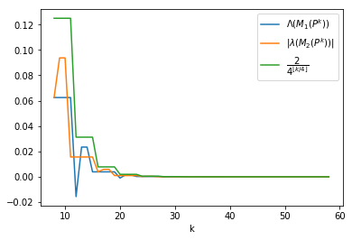
(a) Plot of $\Lambda(M_{1}(P^{k})),|\lambda(M_{2}(P^{k}))|,\left(\frac{2}{4^{\lfloor k/4\rfloor}}\right)$ against $k$

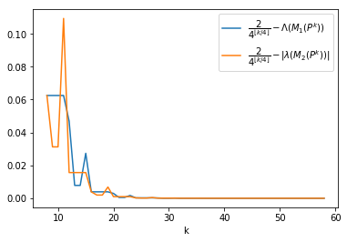
(b) Plot of $\left(\frac{2}{4^{\lfloor k/4\rfloor}}\right)-\Lambda(M_{1}(P^{k})),\left(\frac{2}{4^{\lfloor k/4\rfloor}}\right)-|\lambda(M_{2}(P^{k}))|$ against $k$. The values are all non-negative.

Figure 1. Non-reversible walk on a triangle

Example 5.2 (non-reversible Markov chain sampler).

The second example is taken from Montenegro and Tetali (2006) Example $5.3$ and Diaconis et al. (2000). Consider a Markov chain on $\mathcal{X}=\mathbb{Z}/2m\mathbb{Z}$ labeled by $\{-(m-1),\ldots,0,1,\ldots,m\}$, with transitions $P(i,i+1)=1-\frac{1}{m},P(i,-i)=\frac{1}{m}$. The chain is doubly stochastic with stationary distribution being the uniform distribution on the state space. It is shown in Theorem $1$ of Diaconis et al. (2000) that $t_{mix}(\epsilon)=\Theta(m\log(1/\epsilon))$, and in Montenegro and Tetali (2006) that existing upper bounds cannot provide useful information.

We now fix $m=3$. Finite calculations suggest that we can consider $N_{0}=100$ in (5.3) and (5.4); if this is true, we demonstrate that $\gamma^{ps}$ and $\gamma^{MH}$ both give meaningful bounds. By computation, we have $\gamma^{ps}{\,=\,}\gamma(P^{*3}P^{3})/3=0.315$, and $\gamma^{MH}{\,=\,}1-|\lambda(M_{2}(P^{4}))|^{1/4}=0.270$. Similar to Example 5.1, the upper bound provided by Corollary 5.1 outperforms that in Paulin (2015), since $||P^{k}(x,\cdot)-\pi||_{TV}\leqslant O((1-\gamma^{MH})^{k}){\,=\,}O(0.730^{k})\leqslant O((\sqrt{1-\gamma^{ps}})^{k}){\,=\,}O(\sqrt{0.685}^{k})$.

Next, we consider an example of larger scale and we take $m=100$. Finite calculations again suggest that we can consider $N_{0}=500$ in (5.3) and (5.4). For illustration purposes, we plot $1-\max\{|\lambda(M_{2}(P^{k}))|^{1/k},\Lambda(M_{1}(P^{k}))^{1/k}\}$ and $\gamma(P^{*k}P^{k})/k$ against $k$ in Figure 2. By computation, we see that $\beta^{MH}{\,=\,}0.999914$ and $\gamma^{ps}{\,=\,}0.008671$. In this case, the pseudo-spectral gap performs better than that of MH-spectral gap since $||P^{k}(x,\cdot)-\pi||_{TV}\leqslant O((\sqrt{1-\gamma^{ps}})^{k}){\,=\,}O(0.995655^{k})\leqslant O((1-\gamma^{MH})^{k}){\,=\,}O(0.999914^{k})$. Both bounds are asymptotically tighter than the bound obtained in (Diaconis et al., 2000, Theorem $1$), which gives $||P^{k}(x,\cdot)-\pi||_{TV}\leqslant(1-2^{-7})^{\lfloor k/400\rfloor}$.

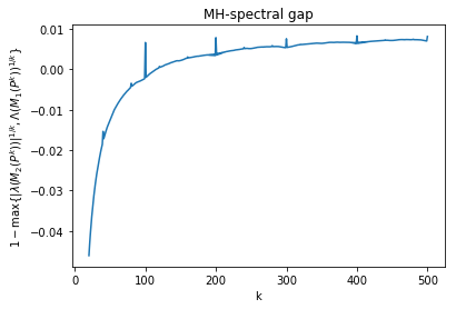
(a) Plot of $1-\max\{|\lambda(M_{2}(P^{k}))|^{1/k},\Lambda(M_{1}(P^{k}))^{1/k}\}$ against $k$

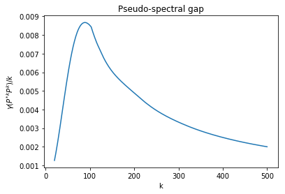
(b) Plot of $\gamma(P^{*k}P^{k})/k$ against $k$

Figure 2. Non-reversible Markov chain sampler with $m=100$ and $N_{0}=500$

Example 5.3 (winning streak).

The third example is the so-called winning streak Markov chain. It has been studied in Example $4.1.5$ and Section $5.3.5$ in Levin et al. (2009). Consider a Markov chain on $\mathcal{X}=\{0,\ldots,m\}$ with transitions $P(i,0)=P(i,i+1)=P(m,m)=1/2$. One remarkable property of such a chain is that its time-reversal, $P^{*}$, attains exactly the stationary distribution in $m$ steps.

By a coupling argument, $d(n)\leqslant\frac{1}{2^{n}}$ for all $m$. Yet, for $P^{*}$, its mixing time is of order $m$. For now we fix $m=4$, and finite calculations suggest that we can consider $N_{0}=100$ in (5.3) and (5.4); if this is true, we have $\gamma^{ps}{\,=\,}\gamma(PP^{*})=0.5$ and $\gamma^{MH}{\,=\,}0.138$, so both the multiplicative reversiblization and pseudo-spectral gap give a correct order of convergence rate. The performance of $\gamma^{MH}$ is poor in this example, due to the fact that $P^{*}$ has a much slower mixing time when compared to $P$.

Next, we consider an example of larger scale and we take $m=50$. Finite calculations again suggest that we can consider $N_{0}=100$ in (5.3) and (5.4). For illustration purposes, we again plot $1-\max\{|\lambda(M_{2}(P^{k}))|^{1/k},\Lambda(M_{1}(P^{k}))^{1/k}\}$ and $\gamma(P^{*k}P^{k})/k$ against $k$ in Figure 3. An interesting feature of the MH-spectral gap plot Figure 3(a) is that $1-\max\{|\lambda(M_{2}(P^{k}))|^{1/k},\Lambda(M_{1}(P^{k}))^{1/k}\}$ rises abruptly to $1$ when $k=m=50$, which should be the case as the chain attains exactly $\pi$ in $m=50$ steps. Such pattern however is missing in the graph of Figure 3(b). By computation, we see that $\beta^{MH}{\,=\,}0.9999$ and $\gamma^{ps}{\,=\,}0.4961$. In this case, the pseudo-spectral gap performs significantly better than that of MH-spectral gap since $||P^{k}(x,\cdot)-\pi||_{TV}\leqslant O((\sqrt{1-\gamma^{ps}})^{k}){\,=\,}O(0.7099^{k})\leqslant O((1-\gamma^{MH})^{k}){\,=\,}O(0.9999^{k})$. Both bounds are asymptotically weaker than the coupling bound as described in the second paragraph above.

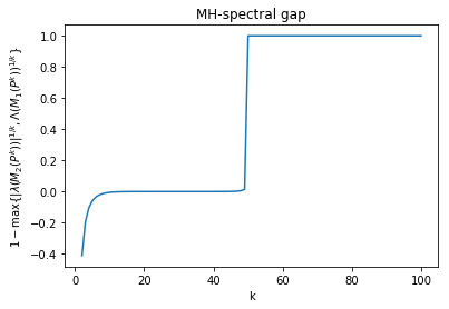
(a) Plot of $1-\max\{|\lambda(M_{2}(P^{k}))|^{1/k},\Lambda(M_{1}(P^{k}))^{1/k}\}$ against $k$

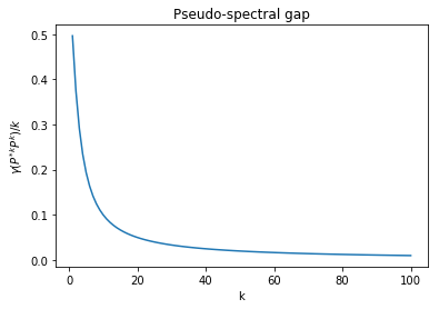
(b) Plot of $\gamma(P^{*k}P^{k})/k$ against $k$

Figure 3. Winning streak Markov chain with $m=50$ and $N_{0}=100$

6. Variance bounds

In this section, we prove variance bounds for Markov chains in terms of the MH-spectral gap. The readers should compare Theorem 6.1 with Lemma $12.20$ in Levin et al. (2009) and Theorem $3.5$,$3.7$ in Paulin (2015).

Theorem 6.1.

Let $(X_{n})_{n\geqslant 0}$ be a Markov chain with Markov kernel $P$, stationary measure $\pi$ and MH-spectral gap $\gamma^{MH}$. Suppose that $f\in L^{2}(\pi)$, and define the variance and asymptotic variance to be respectively

$$V_{f} :=\mathrm{Var}_{\pi}(f),$$

$$\sigma_{as}^{2} :=\lim_{n\to\infty}\dfrac{1}{n}\mathrm{Var}_{\pi}\left(\sum_{i=1}^{n}f(X_{i})\right).$$

The variance bounds are given by

(6.1) $$\mathrm{Var}_{\pi}\left(\sum_{i=1}^{n}f(X_{i})\right) \leqslant nV_{f}\left(|\mathcal{C}^{c}|+\dfrac{2}{\gamma^{MH}}\right),$$

(6.2) $$\bigg{|}\mathrm{Var}_{\pi}\left(\sum_{i=1}^{n}f(X_{i})\right)-n\sigma_{as}^{2}\bigg{|} \leqslant 4V_{f}\left(1+|\mathcal{C}^{c}|+\dfrac{4(\beta^{MH})^{|\mathcal{C}^{c}|+1}}{\gamma^{MH}}\right)^{2}.$$

More generally, if $f_{i}\in L^{2}(\pi)$ for $i=1,\ldots,n$, then

(6.3) $$\mathrm{Var}_{\pi}\left(\sum_{i=1}^{n}f_{i}(X_{i})\right) \leqslant\sum_{i=1}^{n}\mathrm{Var}_{\pi}(f_{i}(X_{i}))\left(|\mathcal{C}^{c}|+\dfrac{2}{\gamma^{MH}}\right).$$

Before we give the proof of Theorem 6.1, we state a lemma that bounds the operator norm of $P$ by that of $M_{1}$ and $M_{2}$ in $L^{2}_{0}(\pi)$.

Lemma 6.1.

Suppose that $P$ is a Markov kernel with stationary measure $\pi$. Then

$$||P||_{L^{2}_{0}(\pi)\to L^{2}_{0}(\pi)}\leqslant||M_{1}||_{L^{2}_{0}(\pi)\to L^{2}_{0}(\pi)}+||M_{2}||_{L^{2}_{0}(\pi)\to L^{2}_{0}(\pi)}+|\lambda(M_{1}(P^{2}))|^{1/2}+|\lambda(M_{2}(P^{2}))|^{1/2}.$$

[Proof. ]By Lemma 3.1(i), we have $||(P+P^{*})f||_{\pi}^{2}=||(M_{1}+M_{2})f||_{\pi}^{2}$ where $f\in L^{2}_{0}(\pi)$. Rearranging the terms give

$$\langle Pf,Pf\rangle_{\pi} =\langle M_{1}f,M_{1}f\rangle_{\pi}+\langle M_{2}f,M_{2}f\rangle_{\pi}+\langle M_{1}f,M_{2}f\rangle_{\pi}+\langle M_{2}f,M_{1}f\rangle_{\pi}$$

$$\quad-\langle P^{*}f,P^{*}f\rangle_{\pi}-\langle f,(P^{*})^{2}f\rangle_{\pi}-\langle f,P^{2}f\rangle_{\pi}$$

$$\leqslant\langle M_{1}f,M_{1}f\rangle_{\pi}+\langle M_{2}f,M_{2}f\rangle_{\pi}+\langle M_{1}f,M_{2}f\rangle_{\pi}+\langle M_{2}f,M_{1}f\rangle_{\pi}$$

$$\quad-\langle f,M_{1}(P^{2})f\rangle_{\pi}-\langle f,M_{2}(P^{2})f\rangle_{\pi},$$

where we used that $P^{2}+(P^{*})^{2}=M_{1}(P^{2})+M_{2}(P^{2})$ by Lemma 3.1(i) and $\langle P^{*}f,P^{*}f\rangle_{\pi}\geqslant 0$ in the inequality. Therefore, we have

$$||Pf||_{\pi}\leqslant(||M_{1}||_{L^{2}_{0}(\pi)\to L^{2}_{0}(\pi)}+||M_{2}||_{L^{2}_{0}(\pi)\to L^{2}_{0}(\pi)})||f||_{\pi}+|\lambda(M_{1}(P^{2}))|^{1/2}+|\lambda(M_{2}(P^{2}))|^{1/2}.$$

Result follows by taking supremum over all $f$ with $||f||_{\pi}\leqslant 1$ and $\mathbb{E}_{\pi}f=0$.

[Proof of Theorem 6.1. ] Assume without loss of generality that $\mathbb{E}_{\pi}(f)=0$ and $\mathbb{E}_{\pi}(f_{i})=0$ for $i=1,\ldots,n$. We first show (6.1). Since $X_{0}\sim\pi$ and by Lemma 3.2,

$$\mathbb{E}_{\pi}(f(X_{i})f(X_{j}))=\langle f,P^{|j-i|}f\rangle_{\pi}\leqslant\langle f,M_{1}(P^{|j-i|})f\rangle_{\pi}=\langle f,(M_{1}(P^{|j-i|})-\pi)f\rangle_{\pi}.$$

Summing up $j$ from $1$ to $n$ leads to

$$\mathbb{E}_{\pi}\left(f(X_{i})\sum_{j=1}^{n}f(X_{j})\right) \leqslant\sum_{j=1}^{n}\langle f,(M_{1}(P^{|j-i|})-\pi)f\rangle_{\pi}$$

$$\leqslant\mathbb{E}_{\pi}(f^{2})\sum_{j=1}^{n}||M_{1}(P^{|j-i|})||_{L^{2}_{0}(\pi)\to L^{2}_{0}(\pi)}$$

$$\leqslant V_{f}\left(|\mathcal{C}^{c}|+\sum_{j=1}^{n}(\beta^{MH})^{|j-i|}\right)$$

$$\leqslant V_{f}\left(|\mathcal{C}^{c}|+\dfrac{2}{\gamma^{MH}}\right).$$

(6.1) follows when we sum $i$ from $1$ to $n$. Next, to show (6.3), we observe that

$$\mathbb{E}_{\pi}(f_{i}(X_{i})f_{j}(X_{j})) =\langle f_{i},P^{|j-i|}f_{j}\rangle_{\pi}$$

$$\leqslant\langle f_{i},(M_{1}(P^{|j-i|})-\pi)f_{j}\rangle_{\pi}$$

$$\leqslant||f_{i}||_{\pi}||f_{j}||_{\pi}||M_{1}(P^{|j-i|})||_{L^{2}_{0}(\pi)\to L^{2}_{0}(\pi)}$$

$$\leqslant\dfrac{1}{2}(\mathbb{E}_{\pi}f_{i}^{2}+\mathbb{E}_{\pi}f_{j}^{2})||M_{1}(P^{|j-i|})||_{L^{2}_{0}(\pi)\to L^{2}_{0}(\pi)}.$$

(6.3) follows when we sum $i,j$ from $1$ to $n$, and $\sum_{j=1}^{n}||M_{1}(P^{|j-i|})||_{L^{2}_{0}(\pi)\to L^{2}_{0}(\pi)}\leqslant|\mathcal{C}^{c}|+\dfrac{2}{\gamma^{MH}}$. Finally, we will show (6.2). Following from the proof of Theorem $3.5$ and $3.7$ in Paulin (2015), using the definition of $\sigma_{as}^{2}$, we have

$$\bigg{|}\mathrm{Var}_{\pi}\left(\sum_{i=1}^{n}f(X_{i})\right)-n\sigma_{as}^{2}\bigg{|}=|\langle f,2(I-(P-\pi)^{n-1})(I-(P-\pi))^{-2}f\rangle_{\pi}|.$$

Note that $||I-(P-\pi)^{n-1}||_{L^{2}(\pi)\to L^{2}(\pi)}\leqslant 2$, and by Lemma 6.1,

$$||(I-(P-\pi))^{-1}||_{L^{2}(\pi)\to L^{2}(\pi)} \leqslant\sum_{k=0}^{\infty}||(P-\pi)^{k}||_{L^{2}(\pi)\to L^{2}(\pi)}$$

$$\leqslant 1+|\mathcal{C}^{c}|+\sum_{k=|\mathcal{C}^{c}|+1}^{\infty}||P^{k}||_{L^{2}_{0}(\pi)\to L^{2}_{0}(\pi)}$$

$$\leqslant 1+|\mathcal{C}^{c}|+4\sum_{k=|\mathcal{C}^{c}|+1}^{\infty}(\beta^{MH})^{k}$$

$$=1+|\mathcal{C}^{c}|+\dfrac{4(\beta^{MH})^{|\mathcal{C}^{c}|+1}}{\gamma^{MH}}.$$

7. Metastability, conductance and Cheeger’s inequality

In this section, we aim at analyzing metastability, conductance, Cheeger’s inequality and their relationships with the two MH kernels. We begin by briefly recalling these concepts.

Definition 7.1 (Metastability of a set).

Let $A,B\in\mathcal{F}$ be measurable subsets of $\mathcal{X}$. Denote by

$$Q(A,B):=\dfrac{1}{\pi(A)}\int_{A}p(x,B)\,\pi(dx)=\dfrac{\langle P\mathds{1}_{A},\mathds{1}_{B}\rangle_{\pi}}{\langle\mathds{1}_{A},\mathds{1}_{A}\rangle_{\pi}}\,,$$

if $\pi(A)>0$ and $0$ otherwise. $A$ is said to be metastable (resp. invariant) if

$$Q(A,A)\approx 1\,(\mathrm{resp}.~{}Q(A,A)=1)\,.$$

Remark 7.1.

Denote $A^{c}$ to be the complement of $A\subset\mathcal{X}$, then $Q(A,A^{c})$ is also known as the conductance of the set $A$. See Definition 7.4 below.

Note that metastability means “almost invariant", in the sense that $Q(A,A)$ is close to $1$. In reality, we are more interested in measuring the metastability of an arbitrary partition of the state space $\mathcal{X}$, in which we state in the following:

Definition 7.2 (Metastability of a partition).

Suppose that $\mathcal{D}=\{A_{1},\ldots,A_{n}\}$ is a partition of $\mathcal{X}$. The metastability of $\mathcal{D}$ is denoted by

$$m(\mathcal{D}):=\sum_{i=1}^{n}Q(A_{i},A_{i})\,.$$

$\mathcal{D}$ is said to be metastable if $m(\mathcal{D})\approx n$.

The next definition measures the “leakage" of a set $A$ at time $t$, which is first introduced by Davies (1982); Singleton (1984).

Definition 7.3 (Leakage).

The leakage of a set $A\in\mathcal{F}$ at time $t$ is denoted by

$$l(A,t):=\dfrac{||\mathds{1}_{A}-P^{t}\mathds{1}_{A}||_{L^{1}(\pi)}}{2\pi(A)(1-\pi(A))}\,.$$

This can be rewritten as

$$l(A,t)=\int_{\mathcal{X}\backslash A}\left(P^{t}\dfrac{\mathds{1}_{A}}{\pi(A)}\right)(x)\dfrac{\pi(dx)}{1-\pi(A)}\,,$$

measuring the probability of $\mathds{1}_{A}/\pi(A)$ being outside $A$ at time $t$.

Remark 7.2.

Another related measure of bottleneckness is conductance. See Definition 7.4 below.

Next, we introduce a key assumption (see e.g. Davies (1982); Singleton (1984); Huisinga and Schmidt (2006)) that will be used in subsequent sections:

Assumption 7.1.

Suppose that $Q:L^{2}(\pi)\rightarrow L^{2}(\pi)$ is a self-adjoint Markov kernel with $n$ eigenvalues denoted by

$$1=\lambda_{1}>\lambda_{2}\geqslant\ldots\geqslant\lambda_{n}\,.$$

In addition, the spectrum $\sigma(Q)$ of $Q$ is contained in

$$\sigma(Q)\subset[a,b]\cup\{\lambda_{n},\ldots,\lambda_{1}\}\,,$$

where $-1<a\leqslant b<\lambda_{n}$. In this sense, the eigenvalues $\lambda_{1},\ldots,\lambda_{n}$ are called dominant as they are larger than $b$.

If $Q$ is a finite Markov chain, or if $Q$ is geometrically ergodic, or if $Q$ is $V$-uniformly ergodic, then it can be shown that $Q$ satisfies Assumption 7.1, see e.g. Huisinga and Schmidt (2006); Schütte and Sarich (2013). Under Assumption 7.1 with $n=2$, if the eigenvalue $\lambda_{2}$ is “close" to $1$, then this is known as “almost degeneracy", which allows us to partition $\mathcal{X}$ into two metastable regions. This has been the subject of investigation in Davies (1982); Singleton (1984).

Next, we provide a quick review on the notion of conductance and Cheeger’s inequality, which are first introduced to the Markov chain literature in Diaconis and Stroock (1991).

Definition 7.4 (Conductance).

The conductance of the set $A$ is

$$\Phi(A):=Q(A,A^{c})=1-Q(A,A)\,,$$

where $Q(A,A^{c})$ is defined in Definition 7.1. The conductance of the chain is defined to be

$$\Phi_{*}(2):=\min_{A\neq\emptyset,\mathcal{X}}\max\{\Phi(A),\Phi(A^{c})\}=\min_{A:0<\pi(A)\leqslant 1/2}\Phi(A)\,.$$

For $k\in\mathbb{N}$, let $\mathcal{D}_{k}=\{A_{1},\ldots,A_{k}\}$ be the set of $k$-uples of disjoint and $\pi$-non-negligible subsets of $\mathcal{X}$. Then the $k$-way expansion is

$$\Phi_{*}(k):=\min_{(A_{1},\ldots,A_{k})\in\mathcal{D}_{k}}\max_{i\in\llbracket k\rrbracket}\Phi(A_{i})\,.$$

Next, we recall the Cheeger’s inequality and its higher-order variants, which provide a two-sided bound in the spectral gap in terms of the $k$-way expansion, see e.g. Lee et al. (2012) and (Miclo, 2015, Proposition $5$) .

Theorem 7.1 (Higher-order Cheeger’s inequality).

Suppose that $P$ is the Markov kernel of a discrete-time reversible finite Markov chain with eigenvalues $1=\lambda_{1}\geqslant\ldots\geqslant\lambda_{n}$. For $k\in\llbracket n\rrbracket$,

$$\dfrac{1-\lambda_{k}}{2}\leqslant\Phi_{*}(k)\leqslant O(k^{4})\sqrt{1-\lambda_{k}}\,.$$

7.1. Main results

In this section, we demonstrate that, by means of comparison (i.e. Peskun’s ordering as in Lemma 3.2), that existing results on metastability, leakage and Cheeger’s inequality can be readily extended to the non-reversible case. We first give spectral bounds on the metastability of partition, in terms of spectral objects associated with the first and second MH kernel $M_{1}$ and $M_{2}$.

Theorem 7.2 (Metastability).

Suppose that $P$ is the Markov kernel of a non-reversible Markov chain on $\mathcal{X}$, with the first and second MH kernel denoted by $M_{1}$ and $M_{2}$ respectively. In addition, for $i=1,2$, $M_{i}$ satisfies Assumption 7.1 with dominant eigenvalues-eigenvectors denoted by $(\lambda_{j}^{(i)},\phi_{j}^{(i)})_{j=1}^{n}$. For any partition $\mathcal{D}=\{A_{1},\ldots,A_{n}\}$, the metastability of $\mathcal{D}$ is bounded by

(7.1) $$1+\sum_{j=2}^{n}\rho_{j}\lambda_{j}^{(2)}+c\leqslant m(\mathcal{D})\leqslant 1+\sum_{j=2}^{n}\lambda_{j}^{(1)}\,,$$

where $\Gamma$ is the orthogonal projection from $L^{2}(\pi)\to\mathrm{Span}\{\mathds{1}_{A_{1}},\ldots,\mathds{1}_{A_{n}}\}$, $\rho_{j}:=||\Gamma\phi_{j}^{(2)}||_{\pi}^{2}\in[0,1]$ for $j=2,\ldots,n$, and

$$c:=a\left(\sum_{j=2}^{n}1-\rho_{j}\right)\,,$$

with $a$ being defined in Assumption 7.1 for $M_{2}$.

Remark 7.3.

This result should be compared with (Huisinga and Schmidt, 2006, Theorem $2$) and (Schütte and Sarich, 2013, Theorem $5.8$), in which we retrieve the corresponding results since $P=M_{1}=M_{2}$ and hence $\lambda_{j}=\lambda_{j}^{(1)}=\lambda_{j}^{(2)}$ in the reversible case.

The next theorem gives spectral bounds on leakage:

Theorem 7.3 (Leakage).

Suppose that $P$ is the Markov kernel of a non-reversible Markov chain on $\mathcal{X}$, with the first and second MH kernel denoted by $M_{1}$ and $M_{2}$ respectively. In addition, for $i=1,2$ and $t\in\mathbb{N}$, $M_{i}(P^{t})$ satisfies Assumption 7.1 with $n=2$ and dominant eigenvalues-eigenvectors denoted by $(\lambda_{j}^{(i)}(P^{t}),\phi_{j}^{(i)}(P^{t}))_{j=1}^{2}$. If $\{A,B\}$ is a partition of $\mathcal{X}$, then for all $t\in\mathbb{N}$,

$$1-\lambda_{2}^{(1)}(P^{t})\leqslant l(A,t)\leqslant 1-\gamma_{A}^{2}(M_{2}(P^{t}))\lambda_{2}^{(2)}(P^{t})\,,$$

where $\gamma_{A}(M_{i}(P^{t}))=\langle\psi_{A},\phi_{2}^{(i)}(P^{t})\rangle_{\pi}$ for $i=1,2$ and

$$\psi_{A}=\sqrt{\dfrac{\pi(B)}{\pi(A)}}\mathds{1}_{A}-\sqrt{\dfrac{\pi(A)}{\pi(B)}}\mathds{1}_{B}\,.$$

Remark 7.4.

This result should be compared with (Singleton, 1984, Theorem $5$), in which we retrieve the corresponding upper bound in the reversible case since $P=M_{1}=M_{2}$ and hence $\lambda_{j}=\lambda_{j}^{(1)}=\lambda_{j}^{(2)}$.

Finally, we give a version of Cheeger’s inequality in bounding the $k$-way expansion, in terms of the eigenvalues of the two Metropolis kernels. This result should be compared with Theorem 7.1.

Theorem 7.4 (Cheeger’s inequality).

Suppose that $P$ is the Markov kernel of a non-reversible Markov chain on a finite state space $\mathcal{X}$, with the first and second MH kernel denoted by $M_{i}$ and eigenvalues $(\lambda_{j}^{(i)})_{j=1}^{n}$ for $i=1,2$. For $k\in\llbracket n\rrbracket$,

(7.2) $$\dfrac{1-\lambda_{k}^{(1)}}{2}\leqslant\Phi_{*}(k)\leqslant O(k^{4})\sqrt{1-\lambda_{k}^{(2)}}\,.$$

7.2. Proofs

[Proof of Theorem 7.2. ] The key step is the Peskun ordering between $P,M_{1},M_{2}$, which yields, for any $f\in L^{2}(\pi)$, the following inequalities:

(7.3) $$\langle M_{2}f,f\rangle_{\pi}\leqslant\langle Pf,f\rangle_{\pi}\leqslant\langle M_{1}f,f\rangle_{\pi}\,.$$

This allows us to link $m(\mathcal{D})$ to the eigenvalues of $M_{1}$ and $M_{2}$. More precisely, we first show the upper bound of (7.1). Making use of the definition, we have

$$m(\mathcal{D})=\sum_{i=1}^{n}\dfrac{\langle P\mathds{1}_{A_{i}},\mathds{1}_{A_{i}}\rangle_{\pi}}{\langle\mathds{1}_{A_{i}},\mathds{1}_{A_{i}}\rangle_{\pi}}\leqslant\sum_{i=1}^{n}\dfrac{\langle M_{1}\mathds{1}_{A_{i}},\mathds{1}_{A_{i}}\rangle_{\pi}}{\langle\mathds{1}_{A_{i}},\mathds{1}_{A_{i}}\rangle_{\pi}}\leqslant 1+\sum_{j=2}^{n}\lambda_{j}^{(1)}\,,$$

where the first inequality follows from (7.3) with $f=\mathds{1}_{A_{i}}$, and we use (Huisinga and Schmidt, 2006, Theorem $2$) in the second inequality since $M_{1}$ is a self-adjoint Markov kernel satisfying Assumption 7.1. Next, to show the lower bound, using (7.3) again, we arrive at

$$m(\mathcal{D})\geqslant\sum_{i=1}^{n}\langle M_{2}\chi_{A_{i}},\chi_{A_{i}}\rangle_{\pi}\,,$$

where $\chi_{A_{i}}:=\frac{\mathds{1}_{A_{i}}}{\sqrt{\langle\mathds{1}_{A_{i}},\mathds{1}_{A_{i}}\rangle_{\pi}}}$. The remaining part of the proof follows a similar argument as in Huisinga and Schmidt (2006). Denote the orthogonal projection by $\Pi:L^{2}(\pi)\rightarrow\mathrm{Span}\{\phi^{(2)}_{1},\ldots,\phi^{(2)}_{n}\}$ and its orthogonal complement by $\Pi^{\perp}=I-\Pi$. Note that

$$\sum_{i=1}^{n}\langle M_{2}\chi_{A_{i}},\chi_{A_{i}}\rangle_{\pi} =\sum_{i=1}^{n}\langle(M_{2}-aI)(\Pi+\Pi^{\perp})\chi_{A_{i}},\chi_{A_{i}}\rangle_{\pi}+a\sum_{i=1}^{n}\langle\chi_{A_{i}},\chi_{A_{i}}\rangle_{\pi}$$

$$=\sum_{i=1}^{n}\langle(M_{2}-aI)\Pi\chi_{A_{i}},\Pi\chi_{A_{i}}\rangle_{\pi}+\sum_{i=1}^{n}\langle(M_{2}-aI)\Pi^{\perp}\chi_{A_{i}},\Pi^{\perp}\chi_{A_{i}}\rangle_{\pi}+an$$

$$\geqslant\sum_{i=1}^{n}\langle(M_{2}-aI)\Pi\chi_{A_{i}},\Pi\chi_{A_{i}}\rangle_{\pi}+an$$

$$=\sum_{i=1}^{n}\bigg{\langle}\sum_{k=1}^{n}(\lambda_{k}^{(2)}-a)\langle\chi_{A_{i}},\phi_{k}^{(2)}\rangle_{\pi}\phi_{k}^{(2)},\sum_{k=1}^{n}\langle\chi_{A_{i}},\phi_{k}^{(2)}\rangle_{\pi}\phi_{k}^{(2)}\bigg{\rangle}_{\pi}+an$$

$$=\sum_{i=1}^{n}\sum_{k=1}^{n}(\lambda_{k}^{(2)}-a)\langle\chi_{A_{i}},\phi_{k}^{(2)}\rangle_{\pi}^{2}+an=\sum_{k=1}^{n}(\lambda_{k}^{2}-a)||\Gamma\phi_{k}^{(2)}||_{\pi}^{2}+an=1+\sum_{j=2}^{n}\rho_{j}\lambda_{j}^{(2)}+c\,,$$

where the inequality follows from the fact that $(M_{2}-aI)$ is self-adjoint and positive semidefinite, the fourth equality comes from the fact that the set $\{\phi^{(2)}_{1},\ldots,\phi^{(2)}_{n}\}$ is orthonormal, the fifth equality makes use of Parseval’s identity, and we use $\lambda_{1}^{(2)}=1,\phi_{1}^{(2)}=\mathds{1},||\Gamma\phi_{1}^{(2)}||_{\pi}^{2}=1$ in the last equality. The desired result follows.

[Proof of Theorem 7.3. ] Similar to the proof of Theorem 7.2, the crux again lies at the appropriate use of (7.3). First, by (Singleton, 1984, Lemma $4$) and (7.3), we have

$$\langle(I-M_{1}(P^{t}))\psi_{A},\psi_{A}\rangle_{\pi}\leqslant\langle(I-P^{t})\psi_{A},\psi_{A}\rangle_{\pi}=l(A,t)\leqslant\langle(I-M_{2}(P^{t}))\psi_{A},\psi_{A}\rangle_{\pi}\,,$$

so it suffices to show that

(7.4) $$\langle(I-M_{2}(P^{t}))\psi_{A},\psi_{A}\rangle_{\pi} \leqslant 1-\gamma_{A}^{2}(M_{2}(P^{t}))\lambda_{2}^{(2)}(P^{t})\,,$$

(7.5) $$\langle(I-M_{1}(P^{t}))\psi_{A},\psi_{A}\rangle_{\pi} \geqslant 1-\lambda_{2}^{(1)}(P^{t})\,.$$

The rest of the proof is similar to that of (Singleton, 1984, Theorem $5$). For $i=1,2$ and $t\in\mathbb{N}$, denote by $\Pi_{i}(P^{t})$ to be the orthogonal projection $\Pi_{i}(P^{t}):L^{2}(\pi)\rightarrow\mathrm{Span}\{\phi^{(i)}_{1}(P^{t}),\phi^{(i)}_{2}(P^{t})\}$ and its orthogonal complement by $\Pi^{\perp}_{i}(P^{t})=I-\Pi_{i}(P^{t})$. Since $\psi_{A}$ is orthogonal to $\phi_{1}^{(i)}(P^{t})=\mathds{1}$, we have

(7.6) $$\Pi_{i}(P^{t})\psi_{A}=\langle\psi_{A},\phi_{2}^{(i)}(P^{t})\rangle_{\pi}\phi_{2}^{(i)}(P^{t})=\gamma_{A}(M_{i}(P^{t}))\phi_{2}^{(i)}(P^{t})\,.$$

We proceed to show (7.4). Note that

$$\langle(I-M_{2}(P^{t}))\psi_{A},\psi_{A}\rangle_{\pi} =\langle(I-M_{2}(P^{t}))(\Pi_{2}(P^{t})+\Pi^{\perp}_{2}(P^{t}))\psi_{A},\psi_{A}\rangle_{\pi}$$

$$=\gamma_{A}^{2}(M_{2}(P^{t}))(1-\lambda_{2}^{(2)}(P^{t}))+\langle(I-M_{2}(P^{t}))\Pi^{\perp}_{2}(P^{t})\psi_{A},\psi_{A}\rangle_{\pi}$$

$$\leqslant\gamma_{A}^{2}(M_{2}(P^{t}))(1-\lambda_{2}^{(2)}(P^{t}))+\langle\Pi^{\perp}_{2}(P^{t})\psi_{A},\psi_{A}\rangle_{\pi}$$

$$=\gamma_{A}^{2}(M_{2}(P^{t}))(1-\lambda_{2}^{(2)}(P^{t}))+\langle(I-\Pi_{2}(P^{t}))\psi_{A},\psi_{A}\rangle_{\pi}$$

$$=1-\gamma_{A}^{2}(M_{2}(P^{t}))\lambda_{2}^{(2)}(P^{t})\,,$$

where the second equality follows from (7.6) and the inequality follows from Cauchy-Schwartz inequality. Finally, we show (7.5). Using the Rayleigh quotient lower bound on the self-adjoint kernel $I-M_{1}(P^{t})$ yields

$$\langle(I-M_{1}(P^{t}))\psi_{A},\psi_{A}\rangle_{\pi} \geqslant 1-\lambda_{2}^{(1)}(P^{t})\,.$$

[Proof of Theorem 7.4. ] We first show the upper bound of (7.2). We have

$$\Phi(A)=1-Q(A,A)\leqslant 1-\dfrac{\langle M_{2}\mathds{1}_{A},\mathds{1}_{A}\rangle_{\pi}}{\langle\mathds{1}_{A},\mathds{1}_{A}\rangle_{\pi}}=\Phi(A)(M_{2})\leqslant O(k^{4})\sqrt{1-\lambda_{k}^{(2)}}\,,$$

where we apply the Peskun ordering (7.3) in the first inequality and the second inequality comes from the Cheeger’s inequality for reversible chain if $M_{2}$ is Markov. In the general case however, we can write $M_{2}=G+I$, where $G$ is the Markov generator of $M_{2}$, and apply the corresponding version of Cheeger’s inequality for $G$ instead (see e.g. (Miclo, 2015, Theorem $2$)), so the desired upper bound follows from the min-max characterization of the $k$-way expansion. Next, for the lower bound of (7.2), we again use the Peskun ordering (7.3) to get

$$\Phi(A)=1-Q(A,A)\geqslant 1-\dfrac{\langle M_{1}\mathds{1}_{A},\mathds{1}_{A^{c}}\rangle_{\pi}}{\langle\mathds{1}_{A},\mathds{1}_{A}\rangle_{\pi}}=\Phi(A)(M_{1})\geqslant\dfrac{1-\lambda_{k}^{(1)}}{2}\,,$$

where the second inequality follows from the Cheeger’s inequality for reversible chain.

7.3. Examples

In this section, we present an example of asymmetric random walk on $n$-cycle and a numerical example of upward skip-free Markov chain to investigate the sharpness of the spectral bounds presented in Theorem 7.2 and 7.3.

Example 7.1 (Asymmetric random walk on the $n$-cycle).

Recall that we have studied the asymmetric random walk on the $n$-cycle in Example 3.1, in which we adapt the notations therein. In particular, we have $l:=\min\{p,q\}$ and $r:=\max\{p,q\}$. For any partition $\mathcal{D}=\{A_{1},A_{2},\ldots,A_{j}\}$ with $0\leqslant j-1<n/2$, the upper bound in Theorem 7.2 now gives

$$1+\sum_{k=1}^{j-1}1-2l(1-\cos(2\pi k/n)) =j(1-2l)+2l\sum_{k=0}^{j-1}\cos(2\pi k/n)$$

$$=j(1-2l)+2l\left(\dfrac{\sin(\pi j/n)\cos(\pi(j-1)/n)}{\sin(\pi/n)}\right)\,.$$

On the other hand, we have for $j\geqslant 2$,

$$\rho_{j}=||\Gamma\phi_{j}^{(2)}||_{\pi}^{2}=\sum_{k=1}^{j}\sum_{x\in A_{k}}\pi(x)\left(\dfrac{\langle\phi_{j}^{(2)},\mathds{1}_{A_{k}}\rangle_{\pi}}{\pi(A_{k})}\right)^{2} =\sum_{k=1}^{j}\sum_{x\in A_{k}}\dfrac{n}{|A_{k}|^{2}}\langle\phi_{j}^{(2)},\mathds{1}_{A_{k}}\rangle_{\pi}^{2}$$

$$=\sum_{k=1}^{j}\dfrac{1}{n|A_{k}|}\left(\sum_{x\in A_{k}}\cos(2\pi(j-1)x/n)\right)^{2},$$

and $a=1-2r+2r\min_{i\geqslant 2}\cos(2\pi(i-1)/n)$, so the lower bound of 7.2 is readily computable.

Next, we now look at the leakage in Theorem 7.3 with the partition $\mathcal{D}=\{A,B\}$. The lower bound becomes

$$1-\lambda_{2}^{(1)}(P^{t})=2l(1-\cos(2\pi/n))\,,$$

while we note that

$$\langle\psi_{A},\phi_{2}^{(2)}(P)\rangle_{\pi}=\dfrac{1}{n}\left(\sqrt{\dfrac{|B|}{|A|}}\sum_{x\in A}\cos(2\pi x/n)-\sqrt{\dfrac{|A|}{|B|}}\sum_{x\in B}\cos(2\pi x/n)\right)\,,$$

so the upper bound in Theorem 7.3 now reads

$$1-\dfrac{1}{n^{2}}\left(\sqrt{\dfrac{|B|}{|A|}}\sum_{x\in A}\cos(2\pi x/n)-\sqrt{\dfrac{|A|}{|B|}}\sum_{x\in B}\cos(2\pi x/n)\right)^{2}\left(1-2r(1-\cos(2\pi/n))\right)\,.$$

Example 7.2 (Upward skip-free).

We consider an upward skip-free chain on $\{1,2,3,4\}$ with Markov kernel given by

$$P=\begin{pmatrix}0.5&0.5&0&0\\ 0.2&0.6&0.2&0\\ 0.1&0.3&0.5&0.1\\ 0.1&0.2&0.4&0.3\\ \end{pmatrix}$$

with eigenvalues $(1,0.52,0.25,0.13)$. The two Metropolis kernels are

$$M_{1}=\begin{pmatrix}0.6&0.4&0&0\\ 0.2&0.66&0.14&0\\ 0&0.3&0.64&0.06\\ 0&0&0.4&0.6\\ \end{pmatrix},\quad M_{2}=\begin{pmatrix}0.40&0.5&0.09&0.01\\ 0.25&0.54&0.2&0.01\\ 0.1&0.44&0.36&0.1\\ 0.1&0.2&0.7&0\\ \end{pmatrix}\,,$$

with eigenvalues $\lambda^{(1)}=(1,0.74,0.50,0.28)$ and $\lambda^{(2)}=(1,0.37,0.08,-0.16)$ respectively. In Theorem 7.2, we have an upper bound $1+\lambda_{2}^{(1)}=1.74$ and lower bound $1+\rho_{2}\lambda_{2}^{(2)}+c=1+0.09\times 0.37+(-0.16)\times(1-0.09)=0.89$.

First, we consider the partition $\mathcal{D}=\{\{1,2\},\{3,4\}\}$ with $A_{1}=\{1,2\}$ and $A_{2}=\{3,4\}$. We see that

$$m(\mathcal{D})=p(A_{1},A_{1})+p(A_{2},A_{2})=0.87+0.61=1.48\,,$$

which is closer to the upper bound $1.74$. If we instead consider the partition $\mathcal{D}=\{\{1,2,3\},\{4\}\}$ with $A_{1}=\{1,2,3\}$ and $A_{2}=\{4\}$, then

$$m(\mathcal{D})=p(A_{1},A_{1})+p(A_{2},A_{2})=0.98+0.3=1.28\,,$$

which is closer to the lower bound of $0.89$.

Acknowledgements. The author thanks Pierre Patie, the associate editor and three referees for constructive comments that have improved the quality and presentation of the paper. This work was partially supported by NSF Grant DMS-1406599 and the Chinese University of Hong Kong, Shenzhen grant PF01001143.

References

- Aldous and Fill (2002) D. Aldous and J. A. Fill. Reversible Markov Chains and Random Walks on Graphs, 2002. Unfinished monograph, recompiled 2014, available at http://www.stat.berkeley.edu/~aldous/RWG/book.html.
- Bierkens (2016) J. Bierkens. Non-reversible Metropolis-Hastings. Stat. Comput., 26(6):1213–1228, 2016.
- Chen (1996) M. Chen. Estimation of spectral gap for Markov chains. Acta Math. Sinica (N.S.), 12(4):337–360, 1996.
- Choi and Patie (2019) M. Choi and P. Patie. Skip-free Markov chains. Trans. Amer. Math. Soc., 371(10):7301–7342, 2019.
- Davies (1982) E. B. Davies. Metastable states of symmetric Markov semigroups. II. J. London Math. Soc. (2), 26(3):541–556, 1982.
- Diaconis and Stroock (1991) P. Diaconis and D. Stroock. Geometric bounds for eigenvalues of Markov chains. Ann. Appl. Probab., 1(1):36–61, 1991.
- Diaconis et al. (2000) P. Diaconis, S. Holmes, and R. M. Neal. Analysis of a nonreversible Markov chain sampler. Ann. Appl. Probab., 10(3):726–752, 2000.
- Fill (1991) J. A. Fill. Eigenvalue bounds on convergence to stationarity for nonreversible Markov chains, with an application to the exclusion process. Ann. Appl. Probab., 1(1):62–87, 1991.
- Hairer et al. (2014) M. Hairer, A. M. Stuart, and S. J. Vollmer. Spectral gaps for a Metropolis-Hastings algorithm in infinite dimensions. Ann. Appl. Probab., 24(6):2455–2490, 2014.
- Hastings (1970) W. K. Hastings. Monte carlo sampling methods using Markov chains and their applications. Biometrika, 57(1):97–109, 1970.
- Horn and Johnson (2013) R. A. Horn and C. R. Johnson. Matrix analysis. Cambridge University Press, Cambridge, second edition, 2013.
- Huisinga and Schmidt (2006) W. Huisinga and B. Schmidt. Metastability and dominant eigenvalues of transfer operators. In New algorithms for macromolecular simulation, volume 49 of Lect. Notes Comput. Sci. Eng., pages 167–182. Springer, Berlin, 2006.
- Jerison (2013) D. Jerison. General mixing time bounds for finite Markov chains via the absolute spectral gap. arXiv preprint arXiv:1310.8021, 2013.
- Kontoyiannis and Meyn (2012) I. Kontoyiannis and S. P. Meyn. Geometric ergodicity and the spectral gap of non-reversible Markov chains. Probab. Theory Related Fields, 154(1-2):327–339, 2012.
- Lee et al. (2012) J. R. Lee, S. Oveis Gharan, and L. Trevisan. Multi-way spectral partitioning and higher-order Cheeger inequalities. In STOC’12—Proceedings of the 2012 ACM Symposium on Theory of Computing, pages 1117–1130. ACM, New York, 2012.
- Levin et al. (2009) D. A. Levin, Y. Peres, and E. L. Wilmer. Markov chains and mixing times. American Mathematical Society, Providence, RI, 2009.
- Metropolis et al. (1953) N. Metropolis, A. W. Rosenbluth, M. N. Rosenbluth, A. H. Teller, and E. Teller. Equation of state calculations by fast computing machines. Journal of Chemical Physics, 21:1087–1092, 1953.
- Meyn and Tweedie (2009) S. Meyn and R. L. Tweedie. Markov chains and stochastic stability. Cambridge University Press, Cambridge, second edition, 2009. With a prologue by Peter W. Glynn.
- Miclo (2015) L. Miclo. On hyperboundedness and spectrum of Markov operators. Invent. Math., 200(1):311–343, 2015.
- Miclo (2016) L. Miclo. On the Markovian similarity. Preprint, Mar. 2016.
- Montenegro and Tetali (2006) R. Montenegro and P. Tetali. Mathematical aspects of mixing times in Markov chains. Found. Trends Theor. Comput. Sci., 1(3):x+121, 2006.
- Patie and Savov (2018) P. Patie and M. Savov. Spectral expansion of non-self-adjoint generalized Laguerre semigroups. Mem. Amer. Math. Soc., page 179p., 2018.
- Paulin (2015) D. Paulin. Concentration inequalities for Markov chains by Marton couplings and spectral methods. Electron. J. Probab., 20:no. 79, 1–32, 2015.
- Peskun (1973) P. H. Peskun. Optimum Monte-Carlo sampling using Markov chains. Biometrika, 60:607–612, 1973.
- Roberts and Rosenthal (1997) G. O. Roberts and J. S. Rosenthal. Geometric ergodicity and hybrid Markov chains. Electron. Comm. Probab., 2:no. 2, 13–25 (electronic), 1997.
- Roberts and Rosenthal (2004) G. O. Roberts and J. S. Rosenthal. General state space Markov chains and MCMC algorithms. Probab. Surv., 1:20–71, 2004.
- Roberts and Tweedie (1996) G. O. Roberts and R. L. Tweedie. Geometric convergence and central limit theorems for multidimensional Hastings and Metropolis algorithms. Biometrika, 83(1):95–110, 1996.
- Rudolf (2012) D. Rudolf. Explicit error bounds for Markov chain Monte Carlo. Dissertationes Math. 485 (2012), 93 pp, 2012.
- Saloff-Coste (1997) L. Saloff-Coste. Lectures on finite Markov chains. In Lectures on probability theory and statistics (Saint-Flour, 1996), volume 1665 of Lecture Notes in Math., pages 301–413. Springer, Berlin, 1997.
- Schütte and Sarich (2013) C. Schütte and M. Sarich. Metastability and Markov state models in molecular dynamics, volume 24 of Courant Lecture Notes in Mathematics. Courant Institute of Mathematical Sciences, New York; American Mathematical Society, Providence, RI, 2013. Modeling, analysis, algorithmic approaches.
- Singleton (1984) G. Singleton. Asymptotically exact estimates for metastable Markov semigroups. Quart. J. Math. Oxford Ser. (2), 35(139):321–329, 1984.
- Sun et al. (2010) Y. Sun, F. Gomez, and J. Schmidhuber. Improving the asymptotic performance of Markov chain monte-carlo by inserting vortices. In NIPS, pages 2235–2243, USA, 2010.
- Tierney (1998) L. Tierney. A note on Metropolis-Hastings kernels for general state spaces. Ann. Appl. Probab., 8(1):1–9, 1998.