The pseudo-Semimicroscopic Algebraic Cluster Model model: Heavy nuclei

Abstract

The Semimicroscopic Algebraic Cluster Model (SACM) is extended to heavy nuclei, making use of the pseudo-$SU(3)$ model. As a first step, the concept of forbiddenness will be resumed. One consequence of the forbiddenness is that the ground state of a nucleus can in general be described by two internally excited clusters. After that, the pseudo-SACM is formulated. The basis of pseudo-SACM is constructed, defining each cluster within the united nucleus with the same oscillator frequency and deformation of the harmonic oscillator as a mean field and dividing the nucleons in those within the unique and normal orbitals, consistently for both clusters and the united nucleus. As test cases, this model is applied to ²³⁶U $\rightarrow$ ²¹⁰Pb+²⁶Ne and ²²⁴Ra $\rightarrow$ ²¹⁰Pb+¹⁴C. Some spectroscopic factors will be calculated as predictions.

PACS: 02.40.ky, 98.80.-k

1 Introduction

The Semimicroscopic Algebraic Cluster Model (SACM) was introduced in [1, 2] and applied to light nuclei up to the first half in the sd-shell. Later some attempts were made to extend it to heavy nuclei. Many applications of the SACM have been studied since then, for example, a construction of the effective $SU(3)$ irreducible representations (irreps) for heavy nuclei [3], using the Nilsson model, and a study of preferences in radioactive decays and/or fission [4, 5, 6]. More recently [7], with the help of the SACM the spectra of $\alpha$ cluster nuclei, of great interest in astrophysics related to the production of heavy elements, and their spectroscopic factors were calculated. In [8, 9] the phase transition properties of the model were investigated and in [10] the renormalization of the coherent state parameters, used for the geometric mapping, was presented.

Though, in [3] a quite powerful method was presented on how to treat heavy nuclei, it only delivers the ground state, or the first super- and hyper-deformed states [11]. Therefore, it is of interest to look for different procedures to deal also with excited states. One of those is the pseudo-$SU(3)$ model ($\widetilde{SU}(3)$) [12, 13]. In [14, 15] the first attempts have been made to extend the SACM to heavy nuclei, applying this $\widetilde{SU}(3)$ model. Problems arise with not reaching the ground state of the united nucleus, after having coupled the two clusters and the relative motion, which turned out to be forbidden in the approximation of the leading representation. In standard $SU(3)$, for clusters with approximately more than 12 protons or neutrons, there is in general no overlap between the coupled cluster state and the relative motion with the ground state of the united nucleus. This was first pointed out in [16], where the notion of forbiddenness was introduced. There, the forbiddenness is defined as the minimal number of excitation quanta needed in at least one of the clusters, such that an overlap with the united nucleus is possible. Reconsidering the definition of forbiddenness from an alternative angle, we were able to prove [17] that the numbers determined in [16] contained numerical errors. In this contribution we will resume the result briefly.

In [14, 15] a different but equivalent definition to the forbiddenness was given, which will be introduced further below. Also in [14, 15], the separation of nucleons into the unique and normal orbitals in the united nucleus, compared to the ones in each cluster, is not well defined: Distinction is made when one cluster is light, which is then treated within the standard shell model, or both are heavy.

Both models, the $\widetilde{SU}(3)$ and the pseudo-SACM, will be explained briefly in section 2 and the problems related to the direct extension of the pseudo-$SU(3)$ scheme to the SACM are mentioned.

After having introduced the improved determination of the forbiddenness, the properties of the $\widetilde{SU}(3)$ model and the SACM, for light nuclei and in its version for heavy nuclei in [14, 15], will be reviewed. We will proceed in section 3 presenting a possible alternative, namely the pseudo-SACM. In order to show the utility of the pseudo-SACM, in section 4 the new proposal is applied to two systems, namely ²³⁶U $\rightarrow$ ²¹⁰Pb+²⁶Ne and ²²⁴Ra $\rightarrow$ ²¹⁰Pb+¹⁴C. In section 5 conclusions are drawn.

2 The pseudo-SACM

The pseudo-$SU(3)$ model [12, 13] is based on the near degeneracy observed in the Nilsson scheme, when in each harmonic oscillator shell $\eta$ the orbital belonging to the largest spin $j=\eta+\frac{1}{2}$ is skipped from consideration. To the remaining orbitals the redefinition

$$j~{}=~{}l\pm\frac{1}{2} \rightarrow {\tilde{l}}~{}=~{}l\mp\frac{1}{2}$$

$$\eta \rightarrow {\tilde{\eta}}~{}=~{}\eta-1~{}~{}~{},$$ (1)

is applied, where ${\tilde{l}}$ denotes the pseudo-orbital angular momentum and ${\tilde{\eta}}$ the pseudo-shell number. Those orbitals with the same pseudo-orbital angular momentum ${\tilde{l}}$ are nearly degenerate, which implies a very small pseudo-spin-orbit interaction. In addition, the content of the $\widetilde{\eta}$ shell corresponds to the one of $\eta=\widetilde{\eta}$ in the standard shell model. Thus, the shell model for light nuclei can be directly extended to heavy nuclei, using $\widetilde{SU}(3)$ model instead of $SU(3)$ model. The orbitals renamed by the pseudo-orbital spin are called normal orbitals, while those in the orbitals with maximal spin $j=\eta+\frac{1}{2}$ are called unique or intruder levels. Nucleons in these unique orbitals are treated as spectators, i.e., it is supposed that the particles in the intruder levels follow the dynamics of those in the normal orbitals and thus they are not forgotten but rather taken into account through well defined effective charges [18]. The influence of the nucleons in the intruder levels are also indirectly taken into account via the parameters of the model. As an example, the intruders are important to obtain correct collective masses, but because these masses are parameters within the model, the effect is taken into account implicitly. Other effects, as the back-bending mechanism provoked by the decoupling of a fermion pair in the intruder orbitals, are not included in the model.

In [18] the basic assumptions of the $\widetilde{SU}(3)$ model were extended to the pseudo-symplectic model of nuclei, which takes into account the nucleons in the closed shells via inter-shell excitations, while the nucleons in the unique orbitals are treated still as spectators. The effective charges are not parameters, as in the $SU(3)$ model, but represent scaling factors, which has a definite dependence on the total number of nucleons and on the division of these nucleons into those in the unique and normal orbitals. There is a similarity between the SACM and the symplectic model [19], namely that both include excitations of $2\hbar\omega$ in the Hamiltonian.

In the SACM for light nuclei, first the $SU(3)$ irrep are determined in the usual way, i.e. each cluster is represented by an irrep $\left(\lambda_{k},\mu_{k}\right)$ ($k=1,2$) for a two cluster system in their ground state. Adding the number of oscillation quanta in each cluster and comparing them with the number of oscillation quanta of the united nucleus results in a mismatch: The number of oscillation quanta of the united nucleus is larger than the sum of both clusters. Wildermuth [20] showed that the necessary condition to satisfy the Pauli exclusion principle is to add the missing quanta into the relative motion, introducing a minimal number of relative oscillation quanta $n_{0}$. This is known as the Wildermuth condition. However, there are still irreps which are not allowed by the Pauli-exclusion principle.

An elegant solution to it, avoiding cumbersome explicit antisymmetrization of the wave function, was proposed [1, 2], where the SACM was presented for the first time: The coupling of the cluster irreps with the one of the relative motion generates a list of $SU(3)$ irreps, i.e.,

$$\left(\lambda_{1},\mu_{1}\right)\otimes\left(\lambda_{2},\mu_{2}\right)\otimes\left(n_{\pi},0\right) = \sum_{m_{\lambda,\mu}}m_{\lambda,\mu}\left(\lambda,\mu\right)~{}~{}~{},$$ (2)

where $n_{\pi}$ is the number of relative oscillation quanta, limited from below by $n_{0}$ and $m_{\lambda,\mu}$ is the multiplicity of $\left(\lambda,\mu\right)$.

This list of irreps is compared to the one of the shell model. Only those are included in the SACM model space, which have a counterpart in the shell model. In such a way, the Pauli exclusion principle is observed and the model space can be called microscopic.

The word Semi in the name of SACM appears due to the phenomenological character of the Hamiltonian, which is a sum of terms related to single particle energies, quadrupole-quadrupole interactions, angular momentum operators and more. In section 3 the structure of the Hamiltonian will be exposed and explained.

As already mentioned, a first attempt to extend the SACM to heavy nuclei was published in [14, 15]. The procedure is very similar to the one for light nuclei, with the difference that now only nucleons in the normal orbitals are considered. For the case of two heavy clusters, for each cluster the nucleons are filled into the Nilsson scheme at the deformation of the corresponding cluster and the same is done for the parent nucleus. When a unique orbital is filled, the nucleons are excluded from counting, while when a normal orbital is filled they are included. As an alternative to this procedure, we use the deformation of the united nucleus also for the clusters (see further detailed discussion in Section 3). In this manner, filling in the protons and neutrons, each cluster has a given number of nucleons in the normal and in the unique orbitals. The $\widetilde{SU}(3)$ irreps for each cluster are determined, using only the nucleons in the normal orbitals, i.e., restricting to the pseudo-oscillator. These irreps are coupled with each other and the one of the relative oscillator, yielding a list of final irreps similar to (2). The problem with this procedure is that even for one light cluster the obtained list may have no overlap with the ones of the irreps in the united nucleus, though some come closer than others.

In order to be able to deal heavy systems, an alternative definition of the forbiddenness was proposed in [14, 15], where the relation of an irrep to its deformation was exploited. Thus, if an irrep of the list has a similar deformation as the one in the shell model allowed irrep, one can say that it is less forbidden than irreps with a larger difference in the irreps. Therefore, the notion of forbiddenness used in [14, 15] is

$$F = \frac{1}{1+min\left[\sqrt{\Delta n_{1}^{2}+\Delta n_{2}^{2}+\Delta n_{3}^{2}}\right]}~{}~{}~{},$$ (3)

where $\Delta n_{i}=\mid n_{i}-n_{i,k}\mid$ and in contrast to $S$, as defined in [14, 15], we use $F$ because the letter $S$ will be used later on for the spectroscopic factor. The index $i$ refers to the spatial direction of the oscillation and $k$ to the several cluster irreps allowed by the Pauli-exclusion principle in (2). The $n_{i}$ is the number of oscillation quanta in direction $i$. This is a distinct definition of forbiddenness as in [16].

It is important to mention that for the case when the parent nucleus consists of one heavy and a light cluster, the light cluster is treated up to now within the $SU(3)$-model, i.e., a mixture of models ($SU(3)$ and $\widetilde{SU}(3)$) is used, adding to the arbitrariness of dividing the nucleons into those occupying unique or normal orbitals. Also, in general, the number of nucleons in the normal orbitals of the clusters do not match those in the united nucleus. Nevertheless, this concept proved to be quite useful in the understanding of structural preferences in the fission or radioactive decay [4, 5, 21].

In spite of this success, it is to us not very satisfactory to deviate in such an amount from the original version of the SACM, where the Pauli principle was taken into account within the same harmonic oscillator mean field. This is the reason why we started to reanalyze the SACM in its version for heavy nuclei, where the spin-orbit interaction is taken into account effectively within the $\widetilde{SU}(3)$ model.

2.1 A new concept of forbiddenness

In [16] it was shown that putting all missing oscillation quanta only into the relative motion, with increasing mass number of the lightest cluster, from one point on it will not be possible to couple the two clusters with the relative motion to the irrep of the united nucleus, thus, it is forbidden. This property is due to the too large irrep $(n_{\pi},0)$ of the relative motion and $n_{\pi}>n_{0}$ increases quickly with a larger cluster mass.

In heavy nuclei valence protons and neutrons occupy different shells and one has to treat them separately. First, we will resume the equations to solve. One way to solve the problem is to allow excitations of one or two of the clusters and adding the remaining oscillation quanta to the relative motion [1]. The minimum number of oscillation quanta needed, to achieve a final overlap with the ground state irrep of the united nucleus, is called the forbiddenness. Unfortunately, it turned out to be difficult to follow the arguments given in [16] on how to determine the forbiddenness. For this reason, the authors published in [17] a detailed description for the determination of the forbiddenness and we resume the main result only (in heavy nuclei, the quantum number in the equation have to carry an addition index for protons or neutrons):

$$n_{C} = {\rm max}\left[0,\frac{1}{3}\left\{n_{0}-(\lambda-\mu)-(2\lambda_{C}+\mu_{C})\right\}\right]$$ (4)

$$+{\rm max}\left[0,\frac{1}{3}\left\{n_{0}-(\lambda+2\mu)+(\lambda_{C}-\mu_{C})\right\}\right]~{}~{}~{}.$$

In (4) the $n_{C}$ denotes the forbidenness, $(\lambda_{C},\mu_{C})$ the cluster irrep (to which the two clusters are coupled and there may appear several), $n_{0}$ is the Wildermuth condition and $(\lambda,\mu)$ is the final $SU(3)$ irrep of the united nucleus. The total number of quanta $n_{0}$, according to the Wildermuth condition, is the sum of $n_{C}$ and the remaining relative oscillation quanta. For later use, we define $\left(\lambda_{0},\mu_{0}\right)$ as the difference of the final cluster irrep $\left(\lambda^{e}_{C},\mu^{e}_{C}\right)$ to the former one $\left(\lambda_{C},\mu_{C}\right)$ (the letter $e$ stands for excited), via

$$\left(\lambda^{e}_{C},\mu^{e}_{C}\right) = \left(\lambda_{C}+\lambda_{0},\mu_{C}+\mu_{0}\right)~{}~{}~{}.$$ (5)

Eq. (4) can be interpreted as follows: The first term in (4) tells us, that in order to minimize $n_{C}$, we have to maximize $(\lambda_{C}+2\mu_{C})$. The second term tells us that in addition the difference $\left(\lambda_{C}-\mu_{C}\right)$ has to be minimized. The condition of a maximal $(\lambda_{C}+2\mu_{C})$ and a minimal $\left(\lambda_{C}-\mu_{C}\right)$ implies a large compact and oblate configuration of the two-cluster system.

One can achieve these conditions, determining the whole product of $(\lambda_{1},\mu_{1})\otimes(\lambda_{2},\mu_{2})$ and searching for the irrep that corresponds to a large compact structure (large $\left(2\lambda_{C}+\mu_{C}\right)$ but with a maximal difference $\left(\mu_{C}-\lambda_{C}\right)$). For deformed clusters, there is also the possibility to excite it within the $0\hbar\omega$, leading to other individual cluster irreps $(\lambda_{C},\mu_{C})$. One can take the whole 0$\hbar\omega$ space of each cluster and multiply them all, or even one can do it for the proton space and the neutron space for each cluster and then multiply the proton final space with the neutron final space, which has to be done anyhow for heavy nuclei because protons and neutrons are in different shells.

The result (4) is similar in structure for light as for heavy nuclei, changing the $SU(3)$ irreps by their $\widetilde{SU}(3)$ values. Before continuing, we shall discuss the philosophy of the extension of the SACM to the pseudo-SACM model, which addresses the question on how to define a cluster within the pseudo-$\widetilde{SU}(3)$ shell model.

We checked the relation of the definition in (3) to the above definition of the forbiddenness and the qualitative consequences are the same, i.e., what is forbidden in one definition is also forbidden in the other one and the same for the allowed irreps. The difference is the explicit determination of $n_{C}$, using (4).

3 Some basic philosophical changes

In this section, we propose an alternative semimicroscopic description of cluster states in heavy nuclei, which is consistent in the separation of nucleons occupying the normal and unique orbitals, for the two clusters as for the united nucleus.

The main point of the proposal, which we like to stress, is that when the united nucleus is considered as a sum of two clusters, these clusters are defined within the united nucleus and not as individual clusters. This happens already in the SACM for light nuclei: The fundamental scale of the harmonic oscillator of the shell model, $\hbar\omega$, is the same for each cluster and the relative oscillator. For example, in ¹⁶O+$\alpha$ $\rightarrow$ ²⁰Ne, the $\hbar\omega$ used is $45A^{-1/3}-25A^{-2/3}$ = 13.19 MeV [22] for the united nucleus ²⁰Ne, while the value for the free ¹⁶O is 13.92  MeV and for $\alpha$ it is 18.43 MeV. The differences are quite large! The argument why the $\hbar\omega$ value of the united nucleus has to be taken is that the two clusters happen to be formed within the united nucleus, i.e, the same mean field.

In [14, 15] the present approach was followed only partially, certainly not for the criteria of which nucleons are in the normal or unique levels. The light clusters were treated within the $SU(3)$, while the heavy ones are treated within $\widetilde{SU}(3)$ model. This leads to an inconsistent separation of active and non-active nucleons.

We propose that a consistent way is to continue to treat each cluster as an entity within the united nucleus, which means:

• In order to determine the number of nucleons in the normal orbitals, the Nilsson level scheme is used and the orbitals are filled at a fixed deformation. We propose to use the same deformation of the united nucleus also for the clusters.

• The nucleons of the heavy cluster are filled in first. This gives the number of nucleons in normal orbitals for this first cluster. Then, on top of it, the nucleons of the light cluster are filled into the Nilsson scheme until the united nucleus is reached. The number of nucleons in the normal orbitals of this united nucleus minus the number of nucleons in normal orbitals of the heavy cluster gives as a result the number of normal nucleons of the light cluster. This assures that the so-called active nucleons in the united nucleus are equal to the sum of active nucleons of the two clusters. Considering that we are interested either in the pre-formation of a light cluster or in the collision of a light cluster as a projectile, the light cluster is considered always as being added on top of the heavy cluster. This will be important when we construct the model space.

• Once the number of nucleons in the normal orbital for each cluster (${\tilde{A}}_{1}$ and ${\tilde{A}}_{2}$) is obtained, these are filled into the pseudo-shell model.

• The Wildermuth condition is applied to the pseudo-oscillator, i.e., the minimal number of oscillation quanta needed is the difference of the oscillation quanta in the pseudo-oscillator of the united nucleus to the sum of oscillation quanta of the pseudo-oscillator of the two clusters. Analogous as Wildermuth showed [20], the pseudo-shell model of the united nucleus is related by an orthogonal transformation to the two pseudo-shell models of the clusters plus the oscillator for the relative motion. Thus, from a mathematical point of view there is no ambiguity. In fact one can proceed now in the same way as in the SACM for light nuclei, due to the assured match of the overlap of the irreps of the two clusters (though excited) with the relative motion to the leading representation of the parent nucleus.

• States in the united nucleus are described by the product of two clusters, which in general are excited, and the number of quanta which remain in the relative motion.

• The nucleons in the unique orbitals are not forgotten, rather their dynamics are taken into account through a scale factor which can be interpreted as an effective charge and also indirectly through the parameters of the model.

The advantage of this procedure is obvious: The Pauli exclusion principle is maintained and the elegance of the SACM for light nuclei is transferred to heavy nuclei. No practical problems appear, no mixing of different oscillator models is needed and the interpretation remains clear.

3.1 The structure of the Hamiltonian

Concerning the construction of the model space, equation (2), for light clusters, changes to

$$\left({\tilde{\lambda}}_{C},{\tilde{\mu}}_{C}\right)\rightarrow\left({\tilde{\lambda}}^{e}_{C},{\tilde{\mu}}^{e}_{C}\right)$$

$$\left({\tilde{\lambda}}^{e}_{C},{\tilde{\mu}}^{e}_{C}\right)\otimes\left({\tilde{n}}_{r},0\right)=\sum_{m_{{\tilde{\lambda}},{\tilde{\mu}}}}m_{{\tilde{\lambda}},{\tilde{\mu}}}\left({\tilde{\lambda}},{\tilde{\mu}}\right)~{}~{}~{},$$ (6)

for heavy clusters, where $\left({\tilde{\lambda}}^{e}_{C},{\tilde{\mu}}^{e}_{C}\right)$ refers to the excited cluster irrep. No irreps for the individual clusters are mentioned yet, because this is a more complicated matter, involving the cluster irreps for protons and neutron separately, which are afterward coupled to a cluster irrep $\left(\tilde{\lambda}_{C},\tilde{\mu_{C}}\right)$ of the combined system. The index $e$ refers to the excited cluster irrep, as explained in the subsection 2.1 on forbiddenness. The list of the irreps of the $\widetilde{SU}(3)$ model are compared to the shell model irreps of the pseudo-oscillator. Only those irreps which appear in the pseudo-oscillator are included in the $\widetilde{SU}(3)$ model space. However, for heavy systems the model space is still extremely large and one has to apply further simplifications. Because this is a matter for itself, the details will be explained in subsection 3.3. There, we will propose further restrictions on how to reduce the size of the model space, using physical arguments.

The most general algebraic Hamiltonian has the same structure as for light nuclei, except that the operators (number operator, quadrupole operator, etc.) are substituted by their pseudo-counter parts. How this is done, is explained in detail in [23], where the mapping is explicitly given. Also, in the $SU(3)$-part an additional term is added, proportional to the square of the second order Casimir operator of the $SU(3)$-group. This was necessary in order to describe some non-linearities in the spectrum.

For deformed nuclei, the $SU(3)$ limit should be a good approximate symmetry. Because in Section 4 we discuss well deformed final nuclei and to illustrate the application, we restrict to the $SU(3)$ symmetry limit. In spite of this limitation, in what follows we present the general structure of the Hamiltonian for a two-cluster system. Further, more general applications, will be presented in future.

The model Hamiltonian has the following structure:

$${\mbox{\boldmath$H$}}=xy{\mbox{\boldmath$H$}}_{\widetilde{SU}(3)}+y(1-x){\mbox{\boldmath$H$}}_{\widetilde{SO}(4)}+(1-y){\mbox{\boldmath$H$}}_{\widetilde{SO}(3)}\>\>\>,$$ (7)

with $x$ and $y$ being mixing parameters of the dynamical symmetries with values between 0 and 1 and

$${\mbox{\boldmath$H$}}_{\widetilde{SU}(3)} = \hbar\omega\mbox{\boldmath$\widetilde{n}$}_{\pi}+a_{4}\mathit{\widetilde{C}}_{2}\left(\widetilde{\lambda}_{C},\widetilde{\mu}_{C}\right)$$

$$+(a_{2}-a_{5}\Delta\mbox{\boldmath$\widetilde{n}$}_{\pi})\mathit{\widetilde{C}}_{2}\left(\widetilde{\lambda},\widetilde{\mu}\right)+t_{3}\left[\mathit{\widetilde{C}}_{2}\left(\widetilde{\lambda},\widetilde{\mu}\right)\right]^{2}$$

$$+(a_{1}-a_{6}\Delta\mbox{\boldmath$\widetilde{n}$}_{\pi})\mathit{\widetilde{C}}_{2}\left(\widetilde{{\mbox{\boldmath$n$}}}_{\pi},0\right)+t_{1}\mathit{\widetilde{C}}_{3}\left(\widetilde{\lambda},\widetilde{\mu}\right)$$

$$+\left(a_{3}+a_{L}(-1)^{\widetilde{L}}+a_{Ln}\Delta\widetilde{{\mbox{\boldmath$n$}}}_{\pi}\right){\mbox{\boldmath$\widetilde{L}$}}^{2}+t_{2}{\mbox{\boldmath$\widetilde{K}$}}^{2}$$

$${\mbox{\boldmath$H$}}_{\widetilde{SO}(4)} = a_{4}\mathit{\widetilde{C}}_{2}\left(\widetilde{\lambda}_{C},\widetilde{\mu}_{C}\right)a_{C}{\widetilde{{\mbox{\boldmath$L$}}}_{C}}^{2}+a_{R}^{\left(1\right)}{\widetilde{{\mbox{\boldmath$L$}}_{R}}}^{2}$$

$$+\left(\gamma+a_{L}(-1)^{\widetilde{L}}\right){\widetilde{{\mbox{\boldmath$L$}}}}^{2}$$

$$+\frac{c}{4}\left[(\mbox{\boldmath$\pi$}^{\dagger}\cdot\mbox{\boldmath$\pi$}^{\dagger})-(\sigma^{\dagger})^{2}\right]\left[(\mbox{\boldmath$\pi$}\cdot\mbox{\boldmath$\pi$})-(\sigma)^{2}\right]$$

$${\mbox{\boldmath$H$}}_{\widetilde{SO}(3)} = \hbar\omega\mbox{\boldmath$\widetilde{n}$}_{\pi}+a_{4}\mathit{\widetilde{C}}_{2}\left(\widetilde{\lambda}_{C},\widetilde{\mu}_{C}\right)$$ (8)

$$+a_{C}{\widetilde{{\mbox{\boldmath$L$}}}_{C}}^{2}+a_{R}^{\left(1\right)}{\widetilde{{\mbox{\boldmath$L$}}}}_{R}^{2}$$

$$+\left(\gamma+a_{L}(-1)^{\widetilde{L}}+a_{Ln}\Delta\widetilde{{\mbox{\boldmath$n$}}}_{\pi}\right){\mbox{\boldmath$\widetilde{L}$}}^{2}~{}~{}~{},$$

where $\Delta\widetilde{{\mbox{\boldmath$n$}}}_{\pi}=\widetilde{{\mbox{\boldmath$n$}}}_{\pi}-(n_{0}-n_{C})$, $(n_{0}-n_{C})$ being the minimal number of quanta required by the Pauli principle and the possible effects of the forbiddeness is taken into account by $n_{C}$. The $a_{Clus}$ is the strength of the quadrupole-quadrupole interaction, restricted to the cluster part, while $R$ and $C$ denote the contributions related to the relative and coupled cluster part respectively, and $\widetilde{{\mbox{\boldmath$L$}}}^{2}$ is the total angular momentum operator. The moment of inertia may depend on the excitation in $\tilde{n}_{\pi}$ (excited states may increase their deformation, corresponding to a larger momentum of inertia). The choice of (7) permits the study of phase transitions between, e.g., $\widetilde{SU}(3)$ and $\widetilde{SO}(4)$ (see [8, 9] for light nuclei).

For the case of two spherical clusters, the second-order Casimir operator of the pseudo-$\widetilde{SU(3)}$ is just $\widetilde{{\mbox{\boldmath$n$}}}_{\pi}(\widetilde{{\mbox{\boldmath$n$}}}_{\pi}+3)$. Note that the information about the deformation of the clusters only enters in the $\widetilde{SU}(3)$ dynamical limit.

The first term of the $\widetilde{SU}(3)$ Hamiltonian, $\hbar\omega\mbox{\boldmath$\widetilde{n}$}_{\pi}$, contains the linear invariant operator of the $\widetilde{U}_{R}(3)$ subgroup, and the $\hbar\omega$ is fixed via $(45A^{-1/3}-25A^{-2/3})$ for light nuclei [22], which can also be used for heavy nuclei. For heavy nuclei $\hbar\omega=41A^{-\frac{1}{3}}$ is more common. The $A$ is now the mass number of the real nucleus and not the number ${\tilde{A}}$ of nucleons in the normal orbitals for the united nucleus.

The $\mbox{\boldmath$\widetilde{C}$}_{2}\left(SU(3)\right)$ is the second order Casimir-invariant of the coupled $\widetilde{SU}(3)$ group, having contributions both from the internal cluster part and from the relative motion. It is given by:

$$\mbox{\boldmath$C$}_{2}(\widetilde{SU}(3)) = \frac{1}{4}\mbox{\boldmath$\widetilde{Q}$}^{2}+\frac{3}{4}\mbox{\boldmath$\widetilde{L}$}^{2},$$

$$\rightarrow \left(\widetilde{\lambda}^{2}+\widetilde{\lambda}\widetilde{\mu}+\widetilde{\mu}^{2}+3\widetilde{\lambda}+3\widetilde{\mu}\right),$$

$$\widetilde{Q} = \mbox{\boldmath$\widetilde{Q}$}_{C}+\mbox{\boldmath$\widetilde{Q}$}_{R},$$

$$\widetilde{L} = \mbox{\boldmath$\widetilde{L}$}_{C}+\mbox{\boldmath$\widetilde{L}$}_{R},$$ (9)

where $\widetilde{Q}$ and $\widetilde{L}$ are the quadrupole and angular momentum operator, respectively. The relations of the quadrupole and angular momentum operators to the $\widetilde{C}^{(1,1)}_{2m}$ generators of the $\widetilde{SU}(3)$ group, expressed in terms of $\widetilde{SU}(3)$-coupled $\pi$-boson creation and annihilation operators [24], are:

$$\mbox{\boldmath$\widetilde{Q}$}_{k,2m} = \frac{1}{\sqrt{3}}\widetilde{C}^{(1,1)}_{k2m},$$

$$\mbox{\boldmath$\widetilde{L}$}_{k1m} = \widetilde{C}^{(1,1)}_{k1m},$$

$$\mbox{\boldmath$\widetilde{C}$}^{(1,1)}_{lm} = \sqrt{2}\left[\mbox{\boldmath$\pi$}^{\dagger}\otimes\mbox{\boldmath$\pi$}\right]^{(1,1)}_{lm}.$$ (10)

The operators in (9) and (10) form at the same time part of the electromagnetic transition operators, which are defined in [7].

3.2 Spectroscopic factors

A parametrization of the spectroscopic factor, within the SACM for light nuclei, was given in [25]:

$$S = e^{A+Bn_{\pi}+C{\cal C}_{2}(\lambda_{1},\mu_{1})+D{\cal C}_{2}(\lambda_{2},\mu_{2})+E{\cal C}_{2}(\lambda_{c},\mu_{c})+F{\cal C}_{2}(\lambda,\mu)+G{\cal C}_{3}(\lambda,\mu)+H\Delta n_{\pi}}$$ (11)

$$\mid\langle(\lambda_{1},\mu_{1})\kappa_{1}L_{1},(\lambda_{2},\mu_{2})\kappa_{2}L_{2}\mid\mid(\lambda_{c},\mu_{c})\kappa_{c}L_{c}\rangle_{\varrho_{c}}$$

$$\cdot\langle(\lambda_{c},\mu_{c})\kappa_{c}L_{c},(n_{\pi},0)1l\mid\mid(\lambda,\mu)\kappa L\rangle_{1}\mid^{2}~{}~{}~{}.$$

The parameters were adjusted to experimental values of spectroscopic factors within the p- and sd-shell, reproducing well exact calculations within the $SU(3)$ shell model [26]. For the good agreement, the factor depending on the $SU(3)$-isoscalar factors turned out to be crucial.

For heavy nuclei spectroscopic factors are poorly or not at all known experimentally. Therefore, we have to propose a simplified manageable ansatz, compared to (11), including the forbiddenness.

In what follows, we will try to get an estimate on the parameter $B$: As argued in [25] this term is the result of the relative part of the wave-function, which for zero angular momentum is proportional to $e^{-aR^{2}}\sim e^{-a\frac{\hbar}{\mu\omega}n_{\pi}}$, where $R$ is the relative distance of the two clusters (though, an $e^{-aR}$ ansatz would be more appropriate, but would leave the harmonic oscillator picture) and $a$ has units of $\rm{fm}^{-2}$. The $\mu$ is the reduced mass. Let us restrict to the minimum value $n_{0}$ of $n_{\pi}$. Using the relation of $r_{0}=\sqrt{\frac{\hbar}{\mu\omega}n_{0}}$ [27], where $r_{0}$ is the minimal distance between the clusters, and taking into account that for this case $R=r_{0}$, we obtain $e^{-\mid B\mid n_{0}}$, with $\mid B\mid=a\frac{\hbar}{\mu\omega}$ and $B<0$. When the wave function is at $e^{-1}$ it gives $\mid B\mid=\frac{1}{n_{0}}$. For the nuclei in the sd-shell, the adjustment of the parameters was done for cases with $n_{0}=8$, which corresponds according to the estimation to $B=-0.13$ approximately. This has to be compared to the value $-0.36$ as obtained in [25], i.e., it is only a rough approximation. The most important part of (11) is the factor depending on the $SU(3)$ isoscalar factors and the influence of the exponential factor is not dominant for the relative structure of the spectroscopic factors. Furthermore, only ratios of spectroscopic factors are of importance, which cancel the exponential contribution for states in the $0\hbar\omega$ shell and when the $(n_{0}-nc)$ is large (as it will be). Then, the corrections for $\Delta n_{\pi}$ of the order of one will be negligible. We do not see a possibility to estimate the parameter $A$ in the exponential factor, which represents a normalization of the spectroscopic factor. The other terms in the exponential factor represent corrections to the inter-cluster distance, because they correspond to deformation effects, and the parameters in front turned out to be consistently small.

In light of the above estimation and discussion, for heavy nuclei we propose the same expression as in (11), but due to the not availability of a sufficient number of values of spectroscopic factors (or none at all) for heavy nuclei, we propose the following simplified expression:

$$S = e^{{\tilde{A}}+{\tilde{B}}({\tilde{n}}_{0}-{\tilde{n}}_{C}+\Delta{\tilde{n}}_{\pi})}$$ (12)

$$\mid\langle({\tilde{\lambda}}_{1},{\tilde{\mu}}_{1}){\tilde{\kappa}}_{1}{\tilde{L}}_{1},({\tilde{\lambda}}_{2},{\tilde{\mu}}_{2}){\tilde{\kappa}}_{2}{\tilde{L}}_{2}\mid\mid({\tilde{\lambda}}_{c}+\lambda_{0},{\tilde{\mu}}_{c}+\mu_{0}){\tilde{\kappa}}_{c}{\tilde{L}}_{c}\rangle_{\varrho_{c}}$$

$$\cdot\langle({\tilde{\lambda}}_{c}+\lambda_{0},{\tilde{\mu}}_{c}+\mu_{0}){\tilde{\kappa}}_{c}{\tilde{L}}_{c},({\tilde{n}}_{\pi},0)1{\tilde{l}}\mid\mid({\tilde{\lambda}},{\tilde{\mu}}){\tilde{\kappa}}{\tilde{L}}\rangle_{1}\mid^{2}~{}~{}~{}.$$

The $n_{\pi}$ in the exponential factor was substituted by $[(\tilde{n}_{0}-\tilde{n}_{C})+\Delta n_{\pi}]$. The $({\tilde{n}}_{0}-{\tilde{n}}_{C})$ is the number of relative oscillation quanta in $0\hbar\omega$ ($\tilde{n}_{C}$ are added to the excitation of the clusters). The parameter is estimated as ${\tilde{B}}=-\frac{1}{{(\tilde{n}}_{0}-\tilde{n}_{C})}$. Because we can not determine the parameter ${\tilde{A}}$, as a consequence only ratios of spectroscopic factors are relevant. An additional dependence on $\tilde{n}_{C}$ is contained in the product of reduced coupling coefficients, with the appearance of $\lambda_{0}$ and $\mu_{0}$ (see the definition in (5)).

3.3 Construction of the model space

In this subsection we discuss how to obtain the cluster irreps of the combined proton-neutron system and which further approximations have to be applied in order that the resulting model space is not too large but still contains the main contributions for low lying states.

In a first step, the criteria for the construction of the model space for the proton and neutron part are explained. The procedure is in complete analogy to the one used for light nuclei, where now each orbital state can be occupied only by one type of nucleons (protons or neutrons), one with spin up and another one with spin down. Denoting by $\gamma$ = $p$ or $n$ the proton and neutron part, respectively, each cluster is in the irrep $\left(\lambda^{\gamma}_{i},\mu^{\gamma}_{i}\right)$ (i=1,2). The relative motion within each subset is defined by $\left(\tilde{n}^{\gamma}_{\pi},0\right)$. The ${\tilde{n}}^{\gamma}_{\pi}$ is the total number of relative oscillation quanta. The possible cluster irreps of the combined system are then, in analogy to (2),

$$\left({\tilde{\lambda}}^{\gamma}_{1},{\tilde{\mu}}^{\gamma}_{1}\right)\otimes\left({\tilde{\lambda}}^{\gamma}_{2},{\tilde{\mu}}^{\gamma}_{2}\right)\otimes\left(n^{\gamma}_{\pi},0\right)~{}\rightarrow~{}\left({\tilde{\lambda}}^{\gamma}_{C},{\tilde{\mu}}^{\gamma}_{C}\right)\otimes~{}~{}\left(n^{\gamma}_{\pi},0\right)$$

$$\rightarrow$$

$$\left({\tilde{\lambda}}^{\gamma},{\tilde{\mu}}^{\gamma}\right)~{}~{}~{}.$$ (13)

The tildes refer to the pseudo-$SU(3)$ model.

As stated, this has to be done for each subsystem. The question is now on how to join both systems and obtain a short list of $\widetilde{SU}(3)$ irreps? For explaining the path taken, it is useful to cast the list of irreps in the following manner:

$$\left\{\begin{array}[]{ccc}\left({\tilde{\lambda}}^{p}_{1},{\tilde{\mu}}^{p}_{1}\right)&\left({\tilde{\lambda}}^{p}_{2},{\tilde{\mu}}^{p}_{2}\right)&\left({\tilde{\lambda}}^{p}_{C},{\tilde{\mu}}^{p}_{C}\right)\\ \left({\tilde{\lambda}}^{n}_{1},{\tilde{\mu}}^{n}_{1}\right)&\left({\tilde{\lambda}}^{n}_{2},{\tilde{\mu}}^{n}_{2}\right)&\left({\tilde{\lambda}}^{n}_{C},{\tilde{\mu}}^{n}_{C}\right)\\ \left({\tilde{\lambda}}_{1},{\tilde{\mu}}_{1}\right)&\left({\tilde{\lambda}}_{2},{\tilde{\mu}}_{2}\right)&\left({\tilde{\lambda}}_{C},{\tilde{\mu}}_{C}\right)\end{array}\right\}$$ (17)

$$\left\{\begin{array}[]{ccc}\left({\tilde{\lambda}}^{p}_{C},{\tilde{\mu}}^{p}_{C}\right)&\left({\tilde{n}}^{p}_{\pi},0\right)&\left({\tilde{\lambda}}_{p},{\tilde{\mu}}_{p}\right)\\ \left({\tilde{\lambda}}^{n}_{C},{\tilde{\mu}}^{n}_{C}\right)&\left({\tilde{n}}^{n}_{\pi},0\right)&\left({\tilde{\lambda}}_{n},{\tilde{\mu}}_{n}\right)\\ \left({\tilde{\lambda}}_{C},{\tilde{\mu}}_{C}\right)&\left({\tilde{n}}_{\pi},{\tilde{\mu}}_{\pi}\right)&\left({\tilde{\lambda}},{\tilde{\mu}}\right)\end{array}\right\}~{}~{}~{}.$$ (21)

The upper indices $p$ and $n$ refer to protons and neutrons, respectively, and the index $C$ to the cluster irrep. The notation in curly brackets is intentional because it reflects the coupling of the different irreps in terms of $9-\left(\lambda,\mu\right)$ $SU(3)$ symbols [24].

The first curly bracket indicates how to obtain the total cluster irrep $\left({\tilde{\lambda}}_{C},{\tilde{\mu}}_{C}\right)$ from the cluster irreps of the proton and neutron systems. The information in the third column is used in the first column of the second curly bracket.

If one takes all possibilities into account, the number of combinations increases astronomically, therefore, one has to find more simplifications based on physical arguments. We suggest:

• When the proton fluid is combined with the neutron fluid, one can safely assume that both fluids move coherently. When they do not, the resulting motion corresponds to giant resonances, which are at high energies. In order to describe them, one has to include extra interaction terms. We are not interested, however, in these excitations and thus can assume that both fluids move coherently.

• The assumption of a coherent motion of the proton versus the neutron fluid implies that when a proton irrep is coupled to a neutron irrep, only the stretched representation is taken into account, i.e., $\left({\tilde{\lambda}}_{p},{\tilde{\mu}}_{p}\right)$ $\otimes$ $\left({\tilde{\lambda}}_{n},{\tilde{\mu}}_{n}\right)$ $\rightarrow$ $\left({\tilde{\lambda}}_{p}+{\tilde{\lambda}}_{n},{\tilde{\mu}}_{p}+{\tilde{\mu}}_{n}\right)$. The irreps in general can refer to the individual cluster irreps, the complete cluster irreps, the relative motion, etc. Thus, in (21) we use

  $$\left({\tilde{\lambda}}^{p}_{1},{\tilde{\mu}}^{p}_{1}\right)\otimes\left({\tilde{\lambda}}^{n}_{1},{\tilde{\mu}}^{n}_{1}\right) \rightarrow \left({\tilde{\lambda}}^{p}_{1}+{\tilde{\lambda}}^{n}_{1},{\tilde{\mu}}^{p}_{1}+{\tilde{\mu}}^{n}_{1}\right)~{}=~{}\left(\tilde{\lambda}_{1},\tilde{\mu}_{1}\right)$$

  $$\left({\tilde{\lambda}}^{p}_{2},{\tilde{\mu}}^{p}_{2}\right)\otimes\left({\tilde{\lambda}}^{n}_{2},{\tilde{\mu}}^{n}_{2}\right) \rightarrow \left({\tilde{\lambda}}^{p}_{2}+{\tilde{\lambda}}^{n}_{2},{\tilde{\mu}}^{p}_{2}+{\tilde{\mu}}^{n}_{2}\right)~{}=~{}\left(\tilde{\lambda}_{2},\tilde{\mu}_{2}\right)$$

  $$\left({\tilde{\lambda}}^{p}_{C},{\tilde{\mu}}^{p}_{C}\right)\otimes\left({\tilde{\lambda}}^{n}_{C},{\tilde{\mu}}^{n}_{C}\right) \rightarrow \left({\tilde{\lambda}}^{p}_{C}+{\tilde{\lambda}}^{n}_{C},{\tilde{\mu}}^{p}_{C}+{\tilde{\mu}}^{n}_{C}\right)~{}=~{}\left(\tilde{\lambda}_{C},\tilde{\mu}_{C}\right)$$

  $$\left({\tilde{\lambda}}_{p},{\tilde{\mu}}_{p}\right)\otimes\left({\tilde{\lambda}}_{n},{\tilde{\mu}}_{n}\right) \rightarrow \left({\tilde{\lambda}}_{p}+{\tilde{\lambda}}_{n},{\tilde{\mu}}_{p}+{\tilde{\mu}}_{n}\right)~{}=~{}\left(\tilde{\lambda},\tilde{\mu}\right)$$

  $$\left({\tilde{n}}_{\pi},{\tilde{\mu}}_{\pi}\right) \rightarrow \left({\tilde{n}}^{p}_{\pi}+{\tilde{n}}^{n}_{\pi},0\right)~{}=~{}\left(\tilde{n}_{\pi},0\right)~{}~{}~{},$$ (22)

  i.e., ${\tilde{\mu}}_{\pi}=0$.

• When the forbiddenness is not zero, one has further to change the cluster irreps in the proton and neutron system to the excited cluster irreps as indicated in subsection 2.1. The forbiddenness can only be calculated within each partial sector (protons or neutrons).

With these restrictions, the number of irreps reduce considerably, but may be still too large for handling the calculations. A further cut-off constraint is

• Restrict the number of irreps in each shell $\tilde{n}_{\pi}$ to only the first $n_{irreps}$ with the largest eigenvalue of the second order Casimir operator of $\widetilde{SU}(3)$. Which value to take for the cut-off value $n_{irrep}$ is a matter of choice. The justification is that large irreps have a larger eigenvalue of the second order Casimir operator of $SU(3)$ and thus are lower in energy, taking into account that the coefficient should be negative as the operator is related to the quadrupole-quadrupole interaction.

In the next section we shall illustrate the procedure for two particular cases.

4 Applications

In this section we apply the pseudo-SACM proposed to two sample systems. The first is ²³⁶U $\rightarrow$ ²¹⁰Pb+²⁶Ne and the second one is ²²⁴Ra $\rightarrow$ ²¹⁰Pb+¹⁴C. For illustrative reasons, only the $\widetilde{SU}(3)$ dynamical symmetry limit will be considered, i.e., the united nucleus must be well deformed. A complete investigation, including studies of phase transitions between different dynamical symmetry limits, will be presented in a future publication.

4.1 ²³⁶U $\rightarrow$ ²¹⁰Pb+²⁶Ne

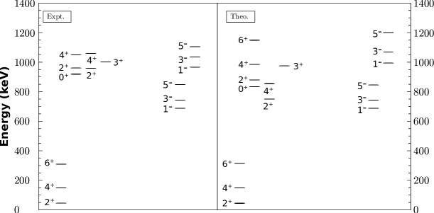
Figure 1: Spectrum of ²³⁶U, described by the clusterization ²¹⁰Pb+²⁶Ne. The theoretical spectrum (right panel) is compared to experiment (left panel).

The protons and neutrons are treated separately and the nucleons in each sector are filled into the Nilsson diagram from below, at the deformation value $\epsilon_{2}=0.200$ [28].

For ²³⁶U, the united nucleus, we obtain 46 protons in the normal orbitals and the valence shell is $\widetilde{\eta}_{p}=4$ with 6 valence protons. The ground state $\widetilde{SU}(3)$ irrep for the proton part is $(\tilde{\lambda},\tilde{\mu})_{\pi}=(18,0)_{\pi}$, while for the neutrons we have 82 particles in normal orbitals with 12 in the $\widetilde{\eta}_{n}=5$ valence shell, giving the ground state irrep $(\tilde{\lambda},\tilde{\mu})_{n}=(36,0)_{n}$. These two irreps can be coupled to the total one for ²³⁶U, namely $(\tilde{\lambda},\tilde{\mu})=(54,0)$. There are, of course, further higher lying $\widetilde{SU}(3)$ irreps in the $0\hbar\omega$ shell. The determination of the ground state irrep is necessary for the evaluation of the forbiddenness (see (4)).

$J_{k}^{P}$	236U: $E_{{\rm exp}}$ [MeV]	224Ra: $E_{{\rm exp}}$ [MeV]
$0_{1}^{+}$	0.0	0.0
$0_{2}^{+}$	0.919	0.916
$0_{3}^{+}$	-	1.223
$2_{1}^{+}$	0.045	0.084
$2_{2}^{+}$	0.958	0.966
$2_{3}^{+}$	1.094	-
$2_{4}^{+}$	1.221	-
$3_{1}^{+}$	1.002	-
$4_{1}^{+}$	0.150	0.251
$6_{1}^{+}$	-	0.479
$1_{1}^{-}$	0.688	0.216
$1_{2}^{-}$	0.967	-
$3_{1}^{-}$	0.744	0.290
$J_{i}^{P}\rightarrow J_{f}^{P}$	236U: $B(E2)$ [WU]	224Ra: $B(E2)$ [WU]
$2_{1}\rightarrow 0_{1}$	250.	97.
$4_{1}\rightarrow 2_{1}$	357.	138

Table 1: Experimental data used in the fit of the parameters of the model Hamiltonian. The second column lists the data used for ²³⁶U and the third column for ²²⁴Ra. If no data is mentioned (dash sign), the value is not used in the fit.

Parameter	236U	224Ra
$a_{1}$	0.041682	-2.5370
$a_{2}$	-1.9466	-2.5386
$a_{3}$	0.014976	0.00029037
$a_{4}$	0.46398	-0.017288
$a_{5}$	-0.48563	-0.46653
$a_{6}$	-1.4577	-0.46939
$a_{L}$	-0.0074986	0.012230
$a_{Lnp}$	-0.016851	0.019355
$t_{1}$	0.023152	-1.2773
$t_{2}$	0.17622	0.42323
$t_{3}$	0.0016846	0.06194
$p_{e2}$	1.8382	1.7752
$e^{(2)}_{1}$	3.6213	3.9261
$e^{(2)}_{2}$	1.4332	1.3948

Table 2: List of parameter values obtained from the fit, for ²³⁶U in the second column and for ²²⁴Ra in the third column. Also listed are the effective charges used in the fit. The effective charges are defined in [7], where $e^{(2)}_{k}$ is the effective charge in the quadrupole transition operator for cluster no. $k=1,2$, estimated geometrically, and $p_{e2}$ is a factor describing the deviation from the geometrical estimate. For details, please consult [7].

$J_{i}^{P_{i}}\rightarrow J_{f}^{P_{f}}$	236U (th)	236U (exp)	224Ra (th)	224Ra (exp)
$2_{1}^{+}\rightarrow 0_{1}^{+}$	250.	250.	97.3	97.0
$2_{1}^{+}\rightarrow 2_{2}^{+}$	0.565	-	5.81	-
$4_{1}^{+}\rightarrow 2_{1}^{+}$	356.	357.	138.	138.
$2_{1}^{+}\rightarrow 3_{1}^{+}$	0.831	-	32.0	-
$3_{1}^{+}\rightarrow 4_{1}^{+}$	0.353	-	8.17	-
$1_{1}^{-}\rightarrow 2_{1}^{-}$	545.	-	42.7	-
$3_{1}^{-}\rightarrow 2_{1}^{-}$	310.	-	28.1	-

Table 3: Theoretical calculated $B(E2,J_{i}^{P_{i}}\rightarrow J_{f}^{P_{f}})$ transition values in Weisskopf units, compared to the experimental values, if available. The first column indicates the transition, the second column the theoretical values for ²³⁶U and the third column the corresponding experimental values, if available. The corresponding data for ²²⁴Ra are listed in the last two columns.

$J_{k}^{P}$	236U (th)	224Ra (th)
$0_{1}^{+}$	0.0015	0.0069
$0_{2}^{+}$	0.0015	0.0069
$2_{1}^{+}$	0.0015	0.0063
$2_{2}^{+}$	0.0	0.0063
$4_{1}^{+}$	0.014	0.0048
$4_{2}^{+}$	0.0	0.0048
$1_{1}^{-}$	0.0	0.0065
$2_{1}^{-}$	0.0	0.0058
$3_{1}^{-}$	0.0	0.0055

Table 4: Some spectroscopic factors, divided by $e^{\widetilde{A}}$, of low lying states. In the first column the state considered is listed. The values of the spectroscopic factor for ²³⁶U and ²²⁴Ra are in the second and third column, respectively.

These considerations have to be repeated for the two clusters involved. The largest cluster is ²¹⁰Pb. Filling the protons into the Nilsson diagram, at the same deformation as for the united nucleus, we obtain 40 protons in normal orbitals, where the valence shell is ${\widetilde{\eta}}=3$ and closed, thus the corresponding irrep is $(0,0)_{p}$. For the neutrons one has 72 in normal orbitals with 2 neutrons in the ${\widetilde{N}}=5$ pseudo-shell. The corresponding irrep is $(10,0)_{n}$.

The light cluster ²⁶Ne is put on top of the heavy cluster. We count 6 protons and 10 neutrons in normal orbitals, which gives $(0,2)_{p}$ and $(4,0)_{n}$.

The minimal number of quanta which have to be added in the proton part is 20, corresponding to a $(20,0)_{pR}$ irrep in the relative part. For the neutron part, this number is 40, i.e., an irrep $(40,0)_{nR}$.

In the next step, the proton parts of the clusters are coupled with the relative part of the protons. The same is done for the neutrons. For the proton part, the product $(0,0)_{p}\otimes(0,2)_{p}\otimes(20,0)_{pR}$ contains the proton irrep $(18,0)_{p}$ of the united nucleus, thus, the forbiddenness for the proton part is zero. The situation is different for the neutron part: The product $(10,0)_{n}\otimes(4,0)_{n}\otimes(40,0)_{nR}$ does not contain (36,0), which is the irrep in the united nucleus. This indicates that one has to excite the clusters and the forbiddenness is different from zero. Using the formula (4) we obtain a forbiddennes of $n_{C}=2$. The excitation of the clusters is achieved, changing the irrep of ²⁶Ne from $(4,0)_{n}$ to $(6,0)_{n}$. The relative part is now reduced by two quanta, leaving $(38,0)_{nR}$. With this change, the product $(10,0)_{n}\otimes(6,0)_{n}\otimes(38,0)_{nR}$ now contains the dominant irrep for neutrons in ²³⁶U.

Using the Hamiltonian (7) in the $SU(3)$-dynamical limit, the coefficients are adjusted to the experimental data, listed in Table 1 in the second column. The optimal parameters obtained are listed in Table 2, second column. With these parameters, the spectrum calculated is depicted in Figure 1. The calculated B(E2)-transition values are listed in Table 3, second (theory) and third (experiment) column.

As can be noted, the agreement to experiment is satisfactory and shows the effectiveness of the pseudo-SACM to describe the collective structure of heavy nuclei.

Next, we calculated some spectroscopic factors, listed in Table 4, second column. The Equation (12) was used with the approximation of the parameter $\widetilde{B}$ as $\left(-\frac{1}{{\tilde{n}}_{0}-n_{C}}\right)$. The total number of relative oscillation quanta for the system under study is ${\tilde{n}}_{0}=60$, thus $\widetilde{B}\approx 0.0172$ and the exponential factor in (12) acquires the form $e^{\widetilde{A}-0.0172({\tilde{n}}_{0}-n_{c}+\Delta{\tilde{n}}_{\pi})}$ $\approx$ $(0.983)^{({\tilde{n}}_{0}-n_{c}+\Delta{\tilde{n}}_{\pi})}e^{\widetilde{A}}$. The factor $e^{\widetilde{A}}$ is unknown and thus in Table 4, the ratios of the spectroscopic factors are more trust-worthy. As can be observed, the spectroscopic factors to $\Delta{\tilde{n}}_{\pi}=1$ are suppressed, where we listed values smaller than $10^{-5}$ as zero.

4.2 ²²⁴Ra $\rightarrow$ ²¹⁰Pb+¹⁴C

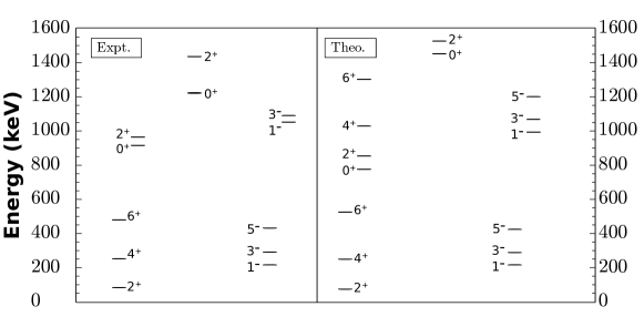
Figure 2: Spectrum of ²²⁴Ra, described by the clusterization ²¹⁰Pb+¹⁴C. The theoretical spectrum (right panel) is compared to experiment (left panel).

As in the former section, the protons and neutrons are treated separately, where the nucleons are filled into the Nilsson diagram from below, at the deformation value $\epsilon_{2}=0.150$ [28].

For ²²⁴Ra, the united nucleus, we obtain 44 protons in the normal orbitals and the valence shell is ${\widetilde{\eta}}_{p}=4$ with 4 valence protons. The $\widetilde{SU}(3)$ irrep is $(\tilde{\lambda},\tilde{\mu})_{p}=(12,2)_{p}$, while for the neutrons we have 78 normal particles with 8 in the ${\widetilde{\eta}}_{n}=5$ valence shell, giving $(\tilde{\lambda},\tilde{\mu})_{n}=(26,4)_{n}$. These two irreps can be coupled to the total one for ²²⁴Ra, namely $(\tilde{\lambda},\tilde{\mu})=(38,6)$.

These considerations have to be repeated for the two clusters involved. The largest cluster is ²¹⁰Pb, with the same numbers as in the former sub-section.

The light cluster ¹⁴C is added on top of the heavy cluster. We count 4 protons and 6 neutrons in normal orbitals, which gives $(2,0)_{p}$ and $(0,2)_{n}$.

The minimal number of quanta which have to be added in the proton part is 14, corresponding to a ($14,0)_{pR}$ irrep in the relative part. For the neutron part, this number is 26, i.e., an irrep $(26,0)_{nR}$.

For the united nucleus, the proton part is coupled separately to the neutron part. For the proton part, the product $(0,0)_{p}\otimes(2,0)_{p}\otimes(14,0)_{pR}$ contains the proton irrep $(12,2)_{p}$ of the united nucleus, thus, the forbiddenness for the proton part is zero. For the neutron part the product $(10,0)_{n}\otimes(0,2)_{n}\otimes(26,0)_{nR}$ does now contain $(26,4)_{n}$, which is the irrep in the united nucleus. This shows that the forbiddenness in this case is zero.

Using the Hamiltonian (7) in the $SU(3)$-dynamical limit, the coefficients are adjusted to the experimental data, listed in Table 1, third column. The optimal parameters obtained are listed in Table 2, third column. With these parameters, the spectrum calculated is depicted in Figure 2. The calculated B(E2)-transition values are listed in Table 3, fourth (theory) and fifth (experiment) column.

As can be noted, the agreement to experiment is satisfactory and shows also in this example the effectiveness of the pseudo-SACM to describe the collective structure of heavy nuclei.

Next, we calculated some spectroscopic factors for ²²⁴Ra, listed in Table 4, third column. The total number of relative oscillation quanta for the system under study is ${\tilde{n}}_{0}=40$ ($n_{C}=0$), thus $\widetilde{B}\approx 0.025$ and the exponential factor in (12) acquires the form $e^{\widetilde{A}-0.025({\tilde{n}}_{0}-n_{c}+\Delta{\tilde{n}}_{\pi})}$ $\approx$ $(0.975)^{({\tilde{n}}_{0}-n_{c}+\Delta{\tilde{n}}_{\pi})}e^{\widetilde{A}}$. The factor $e^{\widetilde{A}}$ is unknown and thus in Table 4, the spectroscopic factors are divided by $e^{A}$. As can be observed, in contrast to ²³⁶U, now the spectroscopic factors to $\Delta{\tilde{n}}_{\pi}=1$ are not suppressed and are of the same order as those to $\Delta{\tilde{n}}_{\pi}=0$.

5 Conclusions

We have presented an extension of the Semimicroscopic Algebraic Cluster Model (SACM), for light nuclei, to the pseudo-SACM, for heavy nuclei. Though, there exist former attempts to extend the SACM to heavy nuclei, we found it necessary to construct a model, which enables us to circumvent some problems of the former approaches and to deliver a more consistent procedure.

In order to extend the SACM to heavy nuclei, several basic assumptions, philosophies and procedures had to be explained, as the concept of forbiddenness, the use of the same deformation and $\hbar\omega$ for the clusters and the united nucleus. Further constraints, as the assumption that the proton and neutron part couple only linearly, were implemented.

For illustrative reasons, the applications were restricted to the dynamical $\widetilde{SU}(3)$ limit. As examples, we considered ²³⁶U $\rightarrow$ ²¹⁰Pb+²⁶Ne and ²²⁴Ra $\rightarrow$ ²¹⁰Pb+¹⁴C. We demonstrated that the model is able to describe the spectrum and electromagnetic transition probabilities. Spectroscopic factors were also calculated, without further fitting and they can be considered as a prediction of the model.

The restriction to the $\widetilde{SU}(3)$ dynamical symmetry limit has to be relaxed in future applications, including the other dynamical symmetries inherit in the Hamiltonian (7). Also the study of phase transitions are of interest, requiring the use of the geometrical mapping [27] of the SACM.

In future, we will also study applications to other heavy systems, especially those where the two clusters are nearly equal. In this case, it is not clear which cluster we have to select first in order to start the filling of the $\widetilde{SU}(3)$ Nilsson levels. The microscopic model space probably will differ slightly when one or the other path is taken, not changing the overall structure.

References

- [1] J. Cseh, Phys. Lett. B 281 (1992), 173.
- [2] J. Cseh and G. Lévai, Ann. Phys. (N.Y.) 230 (1994), 165.
- [3] P. O. Hess, A. Algora, M. Hunyadi, J. Cseh, Eur. Phys. Jour. A15 (2002), 449.
- [4] A. Algora, J. Cseh and P. O. Hess, J. Phys. G 24 (1998), 2111.
- [5] A. Algora, J. Cseh and P. O. Hess, J. Phys. G 25 (1999), 775.
- [6] A. Algora, J. Cseh, J. Darai and P. O. Hess, Phys. Lett. B 639 (2006), 451.
- [7] H. Yépez-Martínez, M. J. Ermamatov, P. R. Fraser and P. O. Hess, Phys. Rev. C 86 (2012), 034309.
- [8] H. Yépez-Martínez, P. R. Fraser, P. O. Hess and G. Lévai, Phys. Rev. C 85 (2012), 014316.
- [9] P. R. Fraser, H. Yépez-Martínez, P. O. Hess and G. Lévai, Phys. Rev. C 85 (2012), 014317.
- [10] H. Yépez-Martínez, G. E. Morales-Hernández, P. O. Hess, G. Lévai and P. R. Fraser, Int. J. Mod. Phys. E 22, no. 4 (2013), 1350022.
- [11] A. Algora, J. Cseh, J. Darai and P.O. Hess, Phys. Lett. B 639 (2006), 451.
- [12] K.T. Hecht and A. Adler, Nucl. Phys. A 137 (1969) 129.
- [13] A. Arima, M. Harvey and K. Shimizu, Phys. Lett. B 30 (1969) 517.
- [14] J. Cseh, R. K. Gupta and W. Scheid, Phys. Lett. B 299 (1993), 205.
- [15] A. Algora and J. Cseh, J. Phys. G 22 (1996), L39.
- [16] Yu. F. Smirnov and Yu. M. Tchuvil’sky, Phys. Lett. B 134 (1984), 25.
- [17] H. Yépez-Martínez, P. O. Hess, J. Phys. G 42 (2015), 095109.
- [18] O.Castaños, P.O.Hess, P.Rocheford, J.P.Draayer, Nucl. Phys. A524 (1991),469-478
- [19] D. J. Rowe, rep. Progr. Phys. 48 (1985), 1419.
- [20] K. Wildermuth and Y. C. Tang, A Unified Theory of the Nucleus (Friedr. Vieweg & Sohn Verlagsgesselschaft mbH, Braunschweig, 1977).
- [21] J. Cseh, A. Algora, J. Darai and P. O. Hess, Phys. Rev. C 70 (2004), 034311.
- [22] J. Blomqvist and A. Molinari, Nucl. Phys. A 106 (1968), 545.
- [23] O. Castaños, J.P. Draayer and Y. Leschber, Ann. of Phys. 180 (1987) 290.
- [24] J. Escher and J.P. Draayer, J. Math. Phys. 39 (1998), 5123.
- [25] P. O. Hess, A. Algora, J. Cseh and J. P. Draayer, Phys. Rev. C70 (2004), 051303(R).
- [26] J. P. Draayer, Nucl. Phys. A 237 (1975), 157.
- [27] P. O. Hess, G. Lévai and J. Cseh, Phys. Rec C 54 (1996) 2345.
- [28] P. Möller, J.R. Nix, W.D. Myers, W.J. Swiatetecki, At. Data Nucl. Data Tables 59 (1995) 185