Lagrangian Descriptors for Two Dimensional, Area Preserving, Autonomous and Nonautonomous Maps

Abstract

In this paper we generalize the method of Lagrangian descriptors to two dimensional, area preserving, autonomous and nonautonomous discrete time dynamical systems. We consider four generic model problems–a hyperbolic saddle point for a linear, area-preserving autonomous map, a hyperbolic saddle point for a nonlinear, area-preserving autonomous map, a hyperbolic saddle point for linear, area-preserving nonautonomous map, and a hyperbolic saddle point for nonlinear, area-preserving nonautonomous map. The discrete time setting allows us to evaluate the expression for the Lagrangian descriptors explicitly for a certain class of norms. This enables us to provide a rigorous setting for the notion that the ‘singular sets” of the Lagrangian descriptors correspond to the stable and unstable manifolds of hyperbolic invariant sets, as well as to understand how this depends upon the particular norms that are used. Finally we analyze, from the computational point of view, the performance of this tool for general nonlinear maps, by computing the “chaotic saddle” for autonomous and nonautonomous versions of the Hénon map.

1 Introduction

Lagrangian descriptors (also referred to in the literature as the ”M function”) were first introduced as a tool for finding hyperbolic trajectories in Madrid and Mancho (2009). In this paper the notion of distinguished trajectory was introduced as a generalization of the well-known idea of distinguished hyperbolic trajectory. The numerical computation of distinguished trajectories was discussed in some detail, and applications to known benchmark examples, as well as to geophysical fluid flows defined as data sets were also given. Later Mendoza and Mancho (2010) showed that it could be used to reveal Lagrangian invariant structures in realistic fluid flows. In particular, a geophysical data set in the region of the Kuroshio current was analysed and it was shown that Lagrangian descriptors could be used to reveal the “Lagrangian skeleton” of the flow, i.e. hyperbolic and elliptic regions, as well as the invariant manifolds that delineate these regions. A deeper study of the Lagrangian transport issue associated with the Kuroshio using Lagrangian descriptors is given in Mendoza and Mancho (2012). Advantages of the method over finite time Lyapunov exponents (FTLE) and finite size Lyapunov exponents (FSLE) were also discussed.

Since then Lagrangian descriptors have been further developed and their ability to reveal phase space structures in dynamical systems more generally has been confirmed. In particular, Lagrangian descriptors are used in de la Cámara et al. (2012) to reveal the Lagrangian structures that define transport routes across the Antarctic polar vortex. Further studies of transport issues related to the Antarctic polar vortex using Lagrangian descriptors are given in de la Cámara et al. (2013) where vortex Rossby wave breaking is related to Lagrangian structures. In Rempel et al. (2013) Lagrangian descriptors are used to study the influence of coherent structures on the saturation of a nonlinear dynamo. In Mendoza et al. (2014) Lagrangian descriptors are used to analyse the influence of Lagrangian structure on the transport of buoys in the Gulf stream and in a region of the Gulf of Mexico relevant to the Deepwater Horizon oil spill. In Mancho et al. (2013) a detailed analysis of the behaviour of Lagrangian descriptors is provided in terms of benchmark problems, new Lagrangian descriptors are introduced, extension of Lagrangian descriptors to 3D flows is given (using the time dependent Hill’s spherical vortex as a benchmark problem), and a detailed analysis and discussion of the computational performance (with a comparison with FTLE) is presented.

Lagrangian descriptors are based on the integration, for a finite time, along trajectories of an intrinsic bounded, positive geometrical and/or physical property of the trajectory itself, such as the norm of the velocity, acceleration, or curvature. Hyperbolic structures are revealed as singular features of the contours of the Lagrangian descriptors, but the sharpness of these singular features depends on the particular norm chosen. These issues were explored in Mancho et al. (2013), and further explored in this paper.

All of the work thus far on Lagrangian descriptors has been in the continuous time setting. In this paper we generalize the method of Lagrangian descriptors to the discrete time setting of two dimensional area preserving maps, both autonomous and nonautonomous, and provide theoretical support for their perfomance.

This paper is organized as follows. In section 2 we defined discrete Lagrangian descriptors. We then consider four examples. In section 2.1 we consider a linear autonomous area preserving map have a hyperbolic saddle point at the origin, in 2.2 we consider a nonlinear autonomous area preserving map have a hyperbolic saddle point at the origin, in 2.3 we consider a linear nonautonomous area preserving map have a hyperbolic saddle trajectory at the origin, and in 2.4 we consider a nonlinear nonautonomous area preserving map have a hyperbolic trajectory at the origin. For each example we show that the Lagrangian descriptors reveal the stable and unstable manifolds by being singular on the manifolds. The notion of “being singular” is made precise in Theorem 1. In section 3 we explore further the method beyond the analytical examples. We use discrete Lagrangian descriptors to computationally reveal the chaotic saddle of the Hénon map, and in section 4 we consider a nonautonomous version of the Hénon map. In section 5 we summarize the conclusions and suggest future directions for this work.

2 Lagrangian Descriptors for Maps

Let

$$\{x_{n},y_{n}\}_{n=-N}^{n=N},\quad N\in\mathbb{N},$$ (1)

denote an orbit of length $2N+1$ generated by a two dimensional map. At this point it does not matter whether or not the map is autonomous or nonautonomous. The method of Lagrangian descriptors applies to orbits in general, regardless of the type of dynamics that generate the orbit.

The first Lagrangian descriptor (also known as the “$M$ function”) for continuous time systems was based on computing the arclength of trajectories for a finite time (Madrid and Mancho (2009)). Extending this idea to maps is straightforward, and the corresponding discrete Lagrangian descriptor (DLD) is given by:

$$MD_{2}=\sum^{N-1}_{i=-N}\sqrt{(x_{i+1}-x_{i})^{2}+(y_{i+1}-y_{i})^{2}}.$$ (2)

In analogy with the work on continuous time Lagrangian descriptors in Mancho et al. (2013), we consider different norms for the discretized arclength as follows:

$$MD_{p}=\sum^{N-1}_{i=-N}\sqrt[p]{|x_{i+1}-x_{i}|^{p}+|y_{i+1}-y_{i}|^{p}},\quad p>1,$$ (3)

and

$$MD_{p}=\sum^{N-1}_{i=-N}|x_{i+1}-x_{i}|^{p}+|y_{i+1}-y_{i}|^{p},\quad p\leq 1.$$ (4)

Considering the space of orbits as a sequence space, (3) and (4) are the $\ell^{p}$ norms of an orbit.

Henceforth, we will consider only the case $p\leq 1$ since the proofs are more simple in this case. Now we will explore these definitions in the context of some easily understood, but generic, examples.

2.1 Example 1: A Hyperbolic Saddle Point for Linear, Area-Preserving Autonomous Maps

2.1.1 Linear Saddle point

Consider the following linear, area-preserving autonomous map:

$$\left\{\begin{array}[]{ccc}x_{n+1}&=&\lambda x_{n},\\ y_{n+1}&=&\frac{1}{\lambda}y_{n},\\ \end{array}\right.$$ (5)

where we will take $\lambda>1$. Note that this map is area-preserving, but area-preservation was not used in the definition of the DLD’s above.

Now we will compute (4) for this example. Towards this end, we introduce the notation

$$MD_{p}=MD^{+}_{p}+MD^{-}_{p}$$

where

$$MD^{+}_{p}=\sum^{N-1}_{i=0}|x_{i+1}-x_{i}|^{p}+|y_{i+1}-y_{i}|^{p},$$

and

$$MD^{-}_{p}=\sum^{-N}_{i=-1}|x_{i+1}-x_{i}|^{p}+|y_{i+1}-y_{i}|^{p}.$$

We begin by computing $MD^{+}_{p}$. The computation of $MD^{-}_{p}$ is completely analogous, and therefore we will not provide the details. We have:

$$MD^{+}_{p} = \displaystyle{\sum^{N-1}_{i=0}|x_{i+1}-x_{i}|^{p}+|y_{i+1}-y_{i}|^{p}}$$

$$= \displaystyle{|x_{1}-x_{0}|^{p}+|y_{1}-y_{0}|^{p}+...+|x_{N}-x_{N-1}|^{p}+|y_{N}-y_{N-1}|^{p}}$$

$$= \displaystyle{|\lambda x_{0}-x_{0}|^{p}+|1/\lambda y_{0}-y_{0}|^{p}+...+|\lambda^{N}x_{0}-\lambda^{N-1}x_{0}|^{p}+|1/\lambda^{N}y_{0}-1/\lambda^{N-1}y_{0}|^{p}}$$

$$= \displaystyle{|x_{0}|^{p}|\lambda-1|^{p}\left(1+\lambda^{p}+...+\lambda^{(N-1)p}\right)+|y_{0}|^{p}|1/\lambda-1|^{p}\left(1+1/\lambda^{p}+...+1/\lambda^{(N-1)p}\right)}$$

$$= \displaystyle{|x_{0}|^{p}|\lambda-1|^{p}\left(\frac{\lambda^{Np}-1}{\lambda^{p}-1}\right)+|y_{0}|^{p}|1/\lambda-1|^{p}\left(\frac{1/\lambda^{Np}-1}{1/\lambda^{p}-1}\right)}$$

where in the last step we have used that the sums are geometric with rates $\lambda^{p}$ and $1/\lambda^{p}$, respectively. By completely analogous calculations we obtain $MD^{-}_{p}$ as:

$$MD^{-}_{p}=|x_{0}|^{p}|1/\lambda-1|^{p}\left(\frac{1/\lambda^{Np}-1}{1/\lambda^{p}-1}\right)+|y_{0}|^{p}|\lambda-1|^{p}\left(\frac{\lambda^{Np}-1}{\lambda^{p}-1}\right).$$

Putting the two terms together, we obtain:

$$\begin{array}[]{ccl}MD_{p}&=&MD^{+}_{p}+MD^{-}_{p}\\ &&\\ &=&(|x_{0}|^{p}+|y_{0}|^{p})(|\lambda-1|^{p}\left(\frac{\lambda^{Np}-1}{\lambda^{p}-1}\right)+|1/\lambda-1|^{p}\left(\frac{1/\lambda^{Np}-1}{1/\lambda^{p}-1}\right))\\ &&\\ &=&(|x_{0}|^{p}+|y_{0}|^{p})f(\lambda,p,N),\\ \end{array}$$ (6)

where $\lambda$, $p$ and $N$ are fixed.

Extensive numerical simulations in a variety of examples (cf. Madrid and Mancho (2009); Mendoza and Mancho (2010); Mendoza et al. (2010); de la Cámara et al. (2012); Mendoza and Mancho (2012); Mancho et al. (2013); Mendoza et al. (2014)) have shown that “singular features” of Lagrangian descriptors correspond to stable and unstable manifolds of hyperbolic trajectories. We can make this statement rigorous and precise in the context of this example.

Theorem 1.

Consider a vertical line perpendicular to the unstable manifold of the origin. In particular, consider an arbitrary point $x=\bar{x}$ and a line parallel to the $y$ axis passing through this point. Then the derivative of $MD_{p}$, $p<1$, along this line becomes unbounded on the unstable manifold of the origin.

Similarly, consider a horizontal line perpendicular to the stable manifold of the origin. In particular, consider an arbitrary point $y=\bar{y}$ and a line parallel to the $x$ axis passing through this point. Then the derivative of $MD_{p}$, $p<1$, along this line becomes unbounded on the stable manifold of the origin.

Proof.

This is a simple calculation using (6) and the fact that $p<1$. This is illustrated in Figure 1. ∎

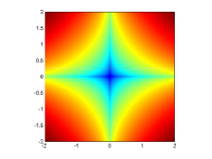
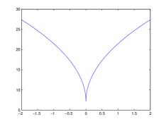
Figure 1: The left-hand panel shows contours of $MD_{p}$ for $p=0.5$, $N=20$ and $\lambda=1.1$, with a grid point spacing of $0.005$. The horizontal black line is at $y=0.25$. The right-hand panel shows the graph of $MD_{p}$ along this horizontal black line, which illustrates the singular nature of the derivative of $MD_{p}$ on the stable manifold across the line $x=0$.

2.1.2 Linear Rotated Saddle point

In the example studied in the previous section the DLD is singular along the stable and unstable manifolds for any iteration $n$. However, the results discussed in Mendoza and Mancho (2010); Mancho et al. (2013) for the continuous time case show that the manifolds are observed for $\tau$ “sufficiently large”, which is related to a large number of iterations in the discrete time case. We explore further these connections by studying the case of the rotated saddle point. In order to establish a direct link to the continuous time case, we consider the limits of small and large numbers of iterations, and $\lambda\approx 1$.

We have the following discrete dynamical system:

$$F(x,y)=A\left(\begin{array}[]{c}x\\ \\ y\\ \end{array}\right)$$ (7)

where

$$A=\left(\begin{array}[]{cc}\frac{1}{\lambda}+\lambda&\frac{1}{\lambda}-\lambda\\ &\\ \frac{1}{\lambda}-\lambda&\frac{1}{\lambda}+\lambda\\ \end{array}\right)=\frac{1}{2\lambda}\left(\begin{array}[]{cc}1+\lambda^{2}&1-\lambda^{2}\\ &\\ 1-\lambda^{2}&1+\lambda^{2}\\ \end{array}\right)$$ (8)

in our case with $\lambda>1$. It is easy to see that the stable and the unstable manifolds are given by the vectors $(1,1)$ and $(1,-1)$ respectively. We want to compute $A^{i}-A^{i-i}$ in order to get the expressions of the DLD:

$$MD_{p}=\sum^{N-1}_{i=-N}|x_{i+1}-x_{i}|^{p}+|y_{i+1}-y_{i}|^{p}$$ (9)

and to find where the ’singularities’ are produced and why.

We know that A can be diagonalized so there exist $D$ and $T$ such that

$$D=T^{-1}\cdot A\cdot T$$ (10)

where $D$ is a diagonal matrix. Therefore we got the next expression

$$D^{i}=T^{-1}\cdot A^{i}\cdot T,\quad\text{for every }i.$$

which is equivalent to

$$A^{i}=T\cdot D^{i}\cdot T^{-1},\quad\text{for every }i.$$ (11)

It is clear that the matrix $T$ is

$$T=\left(\begin{array}[]{cc}1&1\\ -1&1\\ \end{array}\right)$$ (12)

and therefore

$$T^{-1}=\frac{1}{2}\left(\begin{array}[]{cc}1&-1\\ 1&1\\ \end{array}\right)$$

We can check equation (10)

$$\small{D=\frac{1}{4\lambda}\left(\begin{array}[]{ccc}1&&-1\\ &&\\ 1&&1\\ \end{array}\right)\left(\begin{array}[]{cc}1+\lambda^{2}&1-\lambda^{2}\\ &\\ 1-\lambda^{2}&1+\lambda^{2}\\ \end{array}\right)\left(\begin{array}[]{ccc}1&&1\\ &&\\ -1&&1\\ \end{array}\right)=\left(\begin{array}[]{cc}\lambda&0\\ &\\ 0&\frac{1}{\lambda}\\ \end{array}\right)}$$ (13)

So we can guess now how is $A^{i}$ using equation (11)

$$\footnotesize{A^{i}=\frac{1}{2}\left(\begin{array}[]{ccc}1&&1\\ &&\\ -1&&1\\ \end{array}\right)\left(\begin{array}[]{cc}\lambda^{i}&0\\ &\\ 0&\frac{1}{\lambda^{i}}\\ \end{array}\right)\left(\begin{array}[]{ccc}1&&-1\\ &&\\ 1&&1\\ \end{array}\right)=\frac{1}{\lambda^{i}}\left(\begin{array}[]{cc}1+\lambda^{2i}&1-\lambda^{2i}\\ &\\ 1-\lambda^{2i}&1+\lambda^{2i}\\ \end{array}\right)}$$ (14)

Therefore

$$A^{i}-A^{i-1}=\frac{1}{\lambda^{i}}\left(\begin{array}[]{cc}\lambda^{2i}-\lambda^{2i-1}-\lambda+1&-\lambda^{2i}+\lambda^{2i-1}-\lambda+1\\ &\\ -\lambda^{2i}+\lambda^{2i-1}-\lambda+1&\lambda^{2i}-\lambda^{2i-1}-\lambda+1\\ \end{array}\right)$$ (15)

Now we are going to study the analytical expression of the stable and unstable manifold. For that purpose we will develop only $MD^{+}_{p}$ expression ($MD^{-}_{p}$ is analogous). So we have to keep in mind the expression for $MD^{+}_{p}$ that is

$$MD^{+}_{p}=\sum^{N-1}_{i=0}|x_{i+1}-x_{i}|^{p}+|y_{i+1}-y_{i}|^{p}$$ (16)

therefore using equation (15) for $N\geq 1$

$$\scriptsize{\begin{array}[]{rl}MD^{+}_{p}=&\displaystyle{\sum^{N-1}_{i=0}}\frac{1}{\lambda^{(i+1)p}}|(\lambda^{2(i+1)}-\lambda^{2(i+1)-1}-\lambda+1)x_{0}+(-\lambda^{2(i+1)}+\lambda^{2(i+1)-1}-\lambda+1)y_{0}|^{p}\\ &\\ &+\frac{1}{\lambda^{(i+1)p}}|(-\lambda^{2(i+1)}+\lambda^{2(i+1)-1}-\lambda+1)x_{0}+\lambda^{2(i+1)}-\lambda^{2(i+1)-1}-\lambda+1)y_{0}|^{p}\\ \end{array}}$$ (17)

Each term on this sum has singularities along two different lines. In particular, for each $i$ and $\lambda$, we have the two singular lines

$$y_{0}=\frac{\lambda^{2(i+1)}-\lambda^{2(i+1)-1}-\lambda+1}{\lambda^{2(i+1)}-\lambda^{2(i+1)-1}+\lambda-1}x_{0}=m(\lambda,i)x_{0}$$ (18)

and

$$y_{0}=\frac{1}{m(\lambda,n)}x_{0}$$ (19)

where $m(\lambda,i)$ and $\displaystyle{\frac{1}{m(\lambda,i)}}$ are, respectively, the slopes of the singular lines. If we fix $\lambda=\lambda_{0}$ and we increase the number of iterations, we can see the evolution of the singular features to the limit shown in Figure 2

$$\lim_{i\to\infty}m(\lambda_{0},i)=1$$ (20)

This convergence is reached rapidly and, for example, for $\lambda=1.1$ it is noticeable from $i=20$ onwards. Thus at large $i$ most of the terms in the summation (17) contribute with the same slope, i.e., (20), Therefore the contributions of terms in the summation (17) with small $i$ are small and make little impact in the global sum (17). If $i$ is small, the number of terms contributing to the DLD is small, and each term is a $C^{0}$ function with discontinuities along different lines. Since all terms contribute the same to the total pattern, no particular feature is highlighted (see Figure 2b) and 2c)).

The limit $\lambda\approx 1$ is closely related to the Lagrangian Descriptors defined for the continuous time case. This can be seen by considering the limit and noting that $\lambda$ quantifies the separation of points as they are iterated and relating this to the arclength integral for the linear saddle point discussed in Mancho et al. (2013).

For any $i=n_{0}$ fixed, it is possible to find a $\lambda$ in the limit close to 1 that makes the slope $m$ close to the limit value:

$$\lim_{\lambda\to 1}m(\lambda,n_{0})=0$$ (21)

In this case, equations (18) and (19) tend to $y=0$ and $x=0$, respectively. The approach to this limit can be observed in the sequence of images shown Figure 2 and the DLD derivative along the line $y=0.25$ shown in Figure 3.

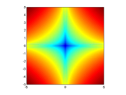
(a) DLD $\lambda=1.1$ and $i=1$

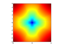
(b) DLD $\lambda=1.1$ and $i=5$

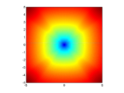
(c) DLD $\lambda=1.1$ and $i=10$

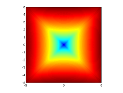
(d) DLD $\lambda=1.1$ and $i=20$

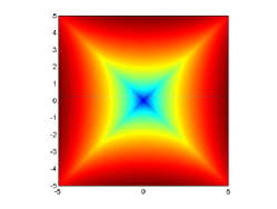
(e) DLD $\lambda=1.1$ and $i=30$

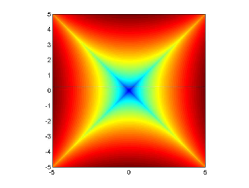
(f) DLD $\lambda=1.1$ and $i=100$

Figure 2: DLD for different values of $\lambda$ and iterations $i$.

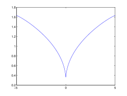
(a) Derivative of the DLD for $\lambda=1.1$ and $i=1$

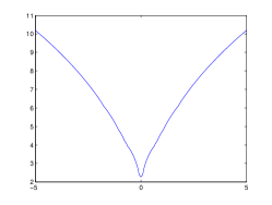
(b) Derivative of the DLD for $\lambda=1.1$ and $i=5$

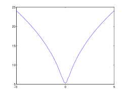
(c) Derivative of the DLD for$\lambda=1.1$ and $i=10$

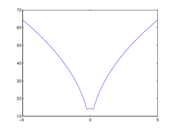
(d) Derivative of the DLD for $\lambda=1.1$ and $i=20$

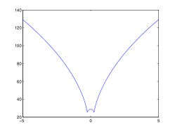
(e) Derivative of the DLD for $\lambda=1.1$ and $i=30$

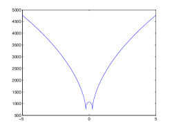
(f) Derivative of the DLD for $\lambda=1.1$ and $i=100$

Figure 3: Derivative of the DLD along the line $y=0.25$ for different values of $\lambda$ and iterations $i$.

2.2 Example 2: A Hyperbolic Saddle Point for Nonlinear, Area-Preserving Autonomous Maps

We will analyze this case using a theorem of Moser (1956). Moser’s theorem applies to analytic, area preserving maps in a neighborhood of a hyperbolic fixed point. We will discuss how the assumptions of analyticity and area preservation can be removed later on, but for now we proceed with these assumptions.

We consider an analytic, area-preserving map in a neighborhood of $x=y=0$ of the form:

$$\left\{\begin{array}[]{ccccc}x_{n+1}&=&f(x_{n},y_{n})&=&\lambda x_{n}+\cdots\\ y_{n+1}&=&g(x_{n},y_{n})&=&\lambda^{-1}y_{n}+\cdots\\ \end{array}\right.$$ (22)

where $\lambda>1$ and ${}^{\prime\prime}\cdots^{\prime\prime}$ represent nonlinear terms that obey the area-preserving constraint. Moser’s Theorem states that there exists a real analytic, area preserving change of variables of the following form:

$$\begin{array}[]{ccccc}x&=&x(\xi,\eta),\\ y&=&y(\xi,\eta),\\ \end{array}$$ (23)

with inverse

$$\begin{array}[]{ccccc}\xi&=&\xi(x,y),\\ \eta&=&\eta(x,y),\\ \end{array}$$ (24)

such that in these new coordinates (22) has the following normal form:

$$\left\{\begin{array}[]{ccl}\xi_{n+1}&=&U(\xi_{n}\eta_{n})\xi_{n}\\ \eta_{n+1}&=&U^{-1}(\xi_{n}\eta_{n})\eta_{n}\\ \end{array}\right.$$ (25)

where $U(\xi\eta)$ is a power series in the product $\xi\eta$ of the form $U_{0}+U_{2}\xi\eta+\cdots$, with $U_{0}=\lambda$, which converges in a neighborhood of the hyperbolic point. Note that it follows from the form of (25) that $U(\cdot)$ is constant on orbits of (25), i.e. $U(\xi_{i+1}\eta_{i+1})=U(\xi_{i}\eta_{i})=U,\forall i$.

The form of (25) implies that the same computation described in Section 2.1 applies. Therefore for $MD^{+}_{p}$ we have:

$$MD^{+}_{p} = \displaystyle{\sum^{N-1}_{i=0}|\xi_{i+1}-\xi_{i}|^{p}+|\eta_{i+1}-\eta_{i}|^{p}}$$

$$= \displaystyle{\sum^{N-1}_{i=0}|\xi_{i}|^{p}|U(\xi_{i}\eta_{i})-1|^{p}+|\eta_{i}|^{p}|U^{-1}(\xi_{i}\eta_{i})-1|^{p}=\sum^{N-1}_{i=0}|\xi_{i}|^{p}|U-1|^{p}+|\eta_{i}|^{p}|U^{-1}-1|^{p}}$$

$$= \displaystyle{|\xi_{0}|^{p}|U-1|^{p}\left(1+|U|^{p}+...+|U|^{(N-1)p}\right)+|\eta_{0}|^{p}|U^{-1}-1|^{p}\left(1+|U^{-1}|^{p}+...+|U^{-1}|^{(N-1)p}\right)}$$

$$= \displaystyle{|\xi_{0}|^{p}|U-1|^{p}\left|\frac{U^{Np}-1}{U^{p}-1}\right|+|\eta_{0}|^{p}|U^{-1}-1|^{p}\left|\frac{1/U^{Np}-1}{1/U^{p}-1}\right|}.$$

$MD^{-}_{p}$ is computed analogously, and therefore $MD_{p}=MD^{+}_{p}+MD^{-}_{p}$ is given by:

$$MD_{p}=\displaystyle{(|\xi_{0}|^{p}+|\eta_{0}|^{p})\left(|U-1|^{p}\left|\frac{U^{Np}-1}{U^{p}-1}\right|+|U^{-1}-1|^{p}\left|\frac{1/U^{Np}-1}{1/U^{p}-1}\right|\right)},$$

In this expression $U$ is constant along trajectories, i.e., $U(\xi_{0}\eta_{0})=U(\xi_{i}\eta_{i})=U,\forall i$. But in general, different initial conditions $(\xi_{0},\eta_{0})$ do not belong to the same trajectory, thus $U$ depends on $(\xi_{0},\eta_{0})$. More succinctly we express this as:

$$\begin{array}[]{ccl}MD_{p}&=&\displaystyle{(|\xi_{0}|^{p}+|\eta_{0}|^{p})f(U(\xi_{0},\eta_{0}),p,N)}\\ \end{array}$$ (26)

This expression has the same form as (6), except for the dependence of the function $f$ on $U(\xi_{0},\eta_{0})$. We note that $U$ is analytical and thus it is a smooth function. Therefore Theorem 1 still applies because the first derivative is infinite due to the first factor in expression (26). We can conclude that the derivative of $MD_{p}$ transverse to the stable manifold is singular on the manifold and the derivative of $MD_{p}$ transverse to the unstable manifold is singular on the manifold. However, this is a statement that is true in the $\xi-\eta$ normal form coordinates. In practice we will compute the Lagrangian descriptor in the original $x-y$ coordinates and therefore we would like to conclude that the “singular sets” of the Lagrangian descriptor in the $x-y$ coordinates correspond to the stable and unstable manifolds of the hyperbolic fixed point. We will now show that this is the case. We will carry out the argument for the the stable manifold. The argument for the unstable manifold is completely analogous.

First, using (23), in the $x-y$ coordinates the stable manifold of the origin is given by the curve $(x(0,\eta),y(0,\eta))$. Here $\eta$ is viewed as a parameter for this parametric representation of the stable manifold in the original $x-y$ coordinates. A vector perpendicular to this curve at any point on the curve is given by $\left(-\frac{dy}{d\eta}(0,\eta),\frac{dx}{d\eta}(0,\eta)\right)$. Now we compute the rate of change of $MD_{p}=MD_{p}(x,y)$ in this direction and consider its behavior on the stable manifold of the origin.This is given by the directional derivative of $MD_{p}(x,y)$ in this direction evaluated on the stable manifold:

$$\left(\frac{\partial MD_{p}}{\partial x}(x(0,\eta),y(0,\eta)),\frac{\partial MD_{p}}{\partial y}(x(0,\eta),y(0,\eta))\right)\cdot\left(-\frac{dy}{d\eta}(0,\eta),\frac{dx}{d\eta}(0,\eta)\right),$$ (27)

where the derivatives are evaluated on $(x(0,\eta),y(0,\eta))$, but we will omit this explicitly for the sake of a less cumbersome notation. Next we will use the chain rule to express partial derivatives with respect to $x$ and $y$ in terms of $\xi$ and $\eta$ as follows:

$$\frac{\partial MD_{p}}{\partial x} = \frac{\partial MD_{p}}{\partial\xi}\frac{\partial\xi}{\partial x}+\frac{\partial MD_{p}}{\partial\eta}\frac{\partial\eta}{\partial x},$$

$$\frac{\partial MD_{p}}{\partial y} = \frac{\partial MD_{p}}{\partial\xi}\frac{\partial\xi}{\partial y}+\frac{\partial MD_{p}}{\partial\eta}\frac{\partial\eta}{\partial y}.$$ (28)

Substituting (28) into (27) gives:

$$-\left(\frac{\partial MD_{p}}{\partial\xi}\frac{\partial\xi}{\partial x}+\frac{\partial MD_{p}}{\partial\eta}\frac{\partial\eta}{\partial x}\right)\frac{dy}{d\eta}+\left(\frac{\partial MD_{p}}{\partial\xi}\frac{\partial\xi}{\partial y}+\frac{\partial MD_{p}}{\partial\eta}\frac{\partial\eta}{\partial y}\right)\frac{dx}{d\eta}.$$ (29)

Now it follows from the argument given in Theorem 1 that $\frac{\partial MD_{p}}{\partial\xi}$ is not differentiable on the stable manifold ($\xi=0$ for $p<1$). Hence (26) is not differentiable in a direction transverse to the stable manifold at a point on the stable manifold in the $x-y$ coordinates.

2.3 Example 3: A Hyperbolic Saddle Point for Linear, Area-Preserving Nonautonomous Maps

In this section we will consider the nonautonomous analog of example 1 in Section 2.1. Namely, we will consider a linear, area preserving nonautonomous map having a hyperbolic trajectory at the origin. The map that we consider has the following form:

$$\left\{\begin{array}[]{ccc}x_{n+1}&=&\lambda_{n}x_{n}\\ y_{n+1}&=&\frac{1}{\lambda_{n}}y_{n}\\ \end{array}\right.$$

where $\lambda_{n}>1,\,\forall n$. Note that $x=y=0$ is a hyperbolic trajectory with stable manifold given by $x=0$ and unstable manifold given by $y=0$ for all $n$.

We will only compute $MD^{+}_{p}$ since the computation of $MD^{-}_{p}$ is analogous. Hence, for $MD^{+}_{p}$ we have:

$$MD^{+}_{p} = \displaystyle{\sum^{N-1}_{i=0}|x_{i+1}-x_{i}|^{p}+|y_{i+1}-y_{i}|^{p}=\sum^{N-1}_{i=0}|x_{i}|^{p}|\lambda_{i}-1|^{p}+|y_{i}|^{p}|1/\lambda_{i}-1|^{p}}$$

$$= \displaystyle{|x_{0}|^{p}\left(|\lambda_{0}-1|^{p}+|\lambda_{0}|^{p}|\lambda_{1}-1|^{p}+...+|\lambda_{0}\cdots\lambda_{N-2}|^{p}|\lambda_{N-1}-1|^{p}\right)+}$$

$$\displaystyle{|y_{0}|^{p}\left(|1/\lambda_{0}-1|^{p}+|1/\lambda_{0}|^{p}|1/\lambda_{1}-1|^{p}+...+|1/\lambda_{0}\cdots 1/\lambda_{N-2}|^{p}|1/\lambda_{N-1}-1|^{p}\right)}$$

$$= \displaystyle{|x_{0}|^{p}\left(|\lambda_{0}-1|^{p}+\sum^{N-1}_{i=1}\left(\prod^{i-1}_{j=0}|\lambda_{j}|^{p}\right)|\lambda_{i}-1|^{p}\right)+}$$

$$\displaystyle{|y_{0}|^{p}\left(|1/\lambda_{0}-1|^{p}+\sum^{N-1}_{i=1}\left(\prod^{i-1}_{j=0}|1/\lambda_{j}|^{p}\right)|1/\lambda_{i}-1|^{p}\right)}$$

A similar calculation gives:

$$MD^{-}_{p} = \displaystyle{|x_{0}|^{p}\left(|1-1/\lambda_{-1}|^{p}+\sum^{-N}_{i=-2}\left(\prod^{i+1}_{j=-1}|1/\lambda_{j}|^{p}\right)|1-1/\lambda_{i}|^{p}\right)}+$$

$$\displaystyle{|y_{0}|^{p}\left(|1-\lambda_{-1}|^{p}+\sum^{-N}_{i=-2}\left(\prod^{i+1}_{j=-1}|\lambda_{j}|^{p}\right)|1-\lambda_{i}|^{p}\right)}.$$

Combining these two expressions gives:

$$\begin{array}[]{ccl}MD_{p}&=&\displaystyle{|x_{0}|^{p}f(\Lambda,p,N)+|y_{0}|^{p}g(\Lambda^{*},p,N)}\\ \end{array}$$ (30)

where

$$\Lambda=(\lambda_{0},\lambda_{1},...,\lambda_{N-1},1/\lambda_{-1},1/\lambda_{-2},...,1/\lambda_{-N})$$

and

$$\Lambda^{*}=(1/\lambda_{0},1/\lambda_{1},...,1/\lambda_{N-1},\lambda_{-1},\lambda_{-2},...,\lambda_{-N}).$$

Now (30) has the same functional form as (6). So for $p<1$ the same argument as given in Theorem 1 holds. Therefore, along a line transverse to the stable manifold (i.e. $x=0$) $MD_{p}$ is not differentiable at the point on this line that intersects the stable manifold. The analogous statement holds for the unstable manifold.

2.4 Example 4: A Hyperbolic Saddle Point for a Nonlinear, Area Preserving Nonautonomous Map

We now consider a two dimensional nonlinear area-preserving nonautonomous map having the following form:

$$x_{n+1} = \lambda_{n}x_{n}+f_{n}(x_{n},y_{n}),$$

$$y_{n+1} = \lambda_{n}^{-1}y_{n}+g_{n}(x_{n},y_{n}),\quad(x_{n},y_{n})\in\mathbb{R}^{2},\forall n,$$ (31)

where $\lambda_{n}>1,\,\forall n$ with $f_{n}(0,0)=g_{n}(0,0)=0,\,\forall n$. We assume that $f_{n}(\cdot,\cdot)$ and $g_{n}(\cdot,\cdot)$ are real valued nonlinear functions (i.e. of order quadratic or higher), they are at least $C^{1}$, and they satisfy the constraints that the nonlinear map defined by (31) is area preserving.

Since the origin is a hyperbolic trajectory it follows that it has (one dimensional) stable and unstable manifolds (Irwin (1973); de Blasi and Schinas (1973); Katok and Hasselblatt (1995)). We will apply the method of discrete Lagrangian descriptors to (31) and show that the stable and unstable manifolds of the origin correspond to the “singular features” of $MD_{p}$ ($p<1$), in the sense described in Theorem 1. Our method of proof will be similar in spirit to how we showed the result for nonlinear autonomous maps by using Moser’s theorem. Unfortunately, there is no analog of Moser’s theorem for nonlinear, nonautonomous area preserving two dimensional maps. Nevertheless, we will still use a “change of variables”, or “conjugation” result that is a nonautonomous map version of the Hartman-Grobman theorem due to Barreira and Valls (2006).

The classical Hartman-Grobman (Hartman (1960b, a, 1963); Grobman (1959, 1962)) theorem applies to autonomous maps in a neighborhood of a hyperbolic fixed point. The result states that there exists a homeomorphism, defined in a neighborhood of the fixed point, which conjugates the map to its linear part. Stated another way, the homeomorphism provides a new set of coordinates where the map is given by its linear part in the new coordinates. There are two issues that we must immediately face in order for this approach to work as it did for the linear and nonlinear autonomous maps. One is the generalization of the Hartman-Grobman theorem to the setting on nonautonomous maps (this is dealt with in Barreira and Valls (2006)) and the other is the smoothness of the conjugation (“change of coordinates”) since a derivative is required in the application of the chain rule (see (28)).

In general, the conjugacy provided by the Hartman-Grobman theorem is not differentiable (see Meyer (1986) for examples). However, there has been much work in determining conditions under which the conjugacy is at least $C^{1}$, see, e.g., van Strien (1990); Guysinsky et al. (2003). Moreover, Hartman has proven (Hartman (1960a)) that in two dimensions, a $C^{2}$ diffeomorphism having a hyperbolic saddle can be linearized with a $C^{1}$ conjugacy (see also Stowe (1986)). We also point out that differentiability is a property defined pointwise, and the nondifferentiability of the conjugacy typically fails to hold at the fixed point (see the examples in Meyer (1986)) and we are not interested in differentiability at the fixed point, but at points along the stable and unstable manifolds of the fixed point. The conjugacy is differentiable at these points, as is described in the lecture notes of Rauch entitled “Conjugacy Outline” availiable at http://www.math.lsa.umich.edu/~rauch/courses.html. This result also follows from the rectification theorem for ordinary differential equations (Arnold (1973)) which says that, away from points where the vector field vanishes, the vector field is conjugate to “rectilinear flow”, and this conjugacy is as smooth as the vector field. Note that this result is valid for both autonomous and nonautonomous vector fields.

So setting aside the smoothness issues, we will give a brief discussion of the set-up of Barreira and Valls (2006) for the nonautonomous Hartman-Grobman theorem. They consider that the phase space is given by a Banach space, denoted $X$ (for us $X$ is $\mathbb{R}^{2}$). The dynamics is described by a sequence of maps on $X$:

$$F_{n}(v)=A_{n}v+f_{n}(v),\quad v\in X,\,n\in\mathbb{Z}.$$ (32)

Precise assumptions on $A_{n}$ and $f_{n}(v)$ are given in Barreira and Valls (2006)). In particular $A_{n}$ is a hyperbolic operator, which for us is:

$$A_{n}=\left(\begin{array}[]{cc}\lambda_{n}&0\\ 0&\lambda_{n}^{-1}\end{array}\right)$$ (33)

and where $f_{n}(v)$ is “small”, in some sense, e.g. $f_{n}(0)=0$ with $f_{n}(v)$ satisfying a Lipschitz condition. Our $f_{n}(v)$ will be at least $C^{1}$ and satisfy the condition for the map (31) to be area preserving.

For each $n\in\mathbb{Z}$ construct a homeomorphism, $h_{n}(\cdot)$ that conjugates (32) to its linear part, i.e.,

$$A_{n}\circ h_{n}=h_{n+1}\circ F_{n},$$ (34)

or, expressing this in a diagram for the full dynamics (following Barreira and Valls (2006)) we have:

$$\begin{array}[]{clclclclc}&&F_{n-1}&&F_{n}&&F_{n+1}&&\\ \longrightarrow&X&\longrightarrow&X&\longrightarrow&X&\longrightarrow&X&\longrightarrow\\ &\downarrow h_{n-1}&&\downarrow h_{n}&&\downarrow h_{n+1}&&\downarrow h_{n+2}&\\ &&A_{n-1}&&A_{n}&&A_{n+1}&&\\ \longrightarrow&X&\longrightarrow&X&\longrightarrow&X&\longrightarrow&X&\longrightarrow\end{array}$$ (35)

In Section 2.3 we proved that the discrete Lagrangian descriptor for the linear, area preserving nonautonomous map is singular along the stable and unstable manifolds of the hyperbolic trajectory at the origin, i.e. $x=0$ and $y=0$, respectively. Note that the discrete Lagrangian descriptor is only a function of the initial condition, $(x_{0},y_{0})$. Hence we can use the change of coordinates $h_{0}(\cdot)$ and the argument given in Section 2.2 to conclude that the discrete Lagrangian descriptor for the nonlinear nonautonomous area preserving map (31) is singular along the stable and unstable manifolds.

3 Application to the Chaotic Saddle of the Hénon Map

We now illustrate the method of discrete Lagrangian descriptors for autonomous, area preserving nonlinear maps by applying it to the Hénon map (Hénon (1976)):

$$H(x,y)=(A+By-x^{2},x).$$ (36)

The map is area preserving for $|B|=1$ and is orientation-preserving if $B<0$. Moreover, it follows from work in Devaney and Nitecki (1979) that for values of $A$ larger than

$$A_{2}=(5+2\sqrt{5})(1+|B|)^{2}/4,$$ (37)

the Hénon map has a hyperbolic invariant Cantor set which is topologically conjugate to a Bernoulli shift on two symbols, i.e. it has a chaotic saddle. We will use the method of discrete Lagrangian descriptors to visualize this chaotic saddle.

We consider $B=-1$, which after substituting this value into (37), gives $A_{2}=5+2\sqrt{5}\approx 9.47$, and therefore we choose $A=9.5$, which satisfies the chaos condition. With these choices of parameters we have $H(x,y)=(9.5-y-x^{2},x)$. Applying the method of discrete Lagrangian descriptors to this map gives the structures shown in Figure 4, where the chaotic saddle is the set that appears as dark blue. This method, in contrast to other techniques for computing chaotic saddles (see for instance Nusse and Yorke (1989)), has the advantage that it simultaneously provides insight into the manifold structure associated with the chaotic saddle.

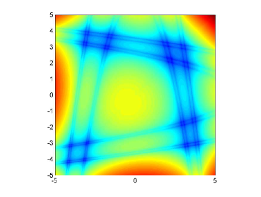
Figure 4: Computation of the chaotic saddle of the Hénon map for $A=9.5,\,B=-1$, after $N=5$ iterations and $p=0.05$.

4 Application to the Chaotic Saddle of a Nonautonomous Hénon Map

We now illustrate the method of discrete Lagrangian descriptors for nonautonomous, area preserving maps by applying it to a nonautonomous version of the Hénon map. In particular, in (36) we take;

$$B=-1,\quad A=9.5+\epsilon\,\cos(n).$$ (38)

For $\epsilon$ ‘small”, this is a nonautonomous perturbation of the situation considered in Section 3, so that we would expect to have a structure similar to that shown in Figure 4, but slightly varying with $n$, i.e. a nonautonomous chaotic saddle (see S.Wiggins (1999)).

The discrete Lagrangian descriptor method provides us with a numerical tool to explore this question. Figure 5 illustrates the phase space structure at different times for the nonautonomous Hénon map. Clearly the output is similar to that shown in Fig. 4, but varying with respect to $n$.

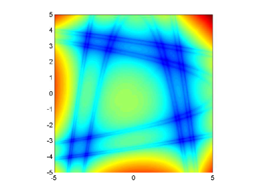
(a) $n=-3$

(b) $n=-1$

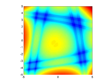
(c) $n=1$

(d) $n=3$

Figure 5: Computation of the chaotic saddle of the nonautonomous Hénon map for $A=9.5+\epsilon\,\cos(n),\,B=-1$, after $N=5$ iterations and $p=0.05$. The output is shown for four different times.

5 Summary and Conclusions

In this paper we have generalized the notion of Lagrangian descriptors to autonomous and nonautonomous maps. We have restricted our discussion to two dimensional, area preserving maps, but with additional work it should be possible to remove these restrictions.

In the discrete time setting explicit expressions for the Lagrangian descriptors were derived, and for the $\ell^{p}$ norm, $p<1$, we proved a theorem that gave rigorous meaning to the statement that “singular sets” of the Lagrangian descriptors correspond to the stable and unstable manifolds of hyperbolic invariant sets.

References

- Arnold (1973) Arnold, V. I. (1973). Ordinary Differential Equations. MIT Press.
- Barreira and Valls (2006) Barreira, L. and Valls, C. (2006). A Grobman–Hartman theorem for nonuniformly hyperbolic dynamics. J. Diff. Eq., 228, 285–310.
- de Blasi and Schinas (1973) de Blasi, F. S. and Schinas, J. (1973). On the stable manifold theorem for discrete time dependent processes in banach spaces. Bull. London Math. Soc., 5, 275–282.
- de la Cámara et al. (2012) de la Cámara, A., Mancho, A. M., Ide, K., Serrano, E., and Mechoso, C. (2012). Routes of transport across the Antarctic polar vortex in the southern spring. J. Atmos. Sci., 69(2), 753–767.
- de la Cámara et al. (2013) de la Cámara, A., Mechoso, C., Mancho, A. M., Serrano, E., and Ide, K. (2013). Quasi-horizontal transport within the antarctic polar night vortex: Rossby wave breaking evidence and lagrangian structures. J. Atmos. Sci., 70, 2982–3001.
- Devaney and Nitecki (1979) Devaney, R. and Nitecki, Z. (1979). Shift automorphisms in the hénon mapping. Comm. Math. Phys., 67, 137–179.
- Grobman (1959) Grobman, D. M. (1959). Homeomorphisms of systems of differential equations. Doklady Akad. Nauk SSSR, 128, 880–881.
- Grobman (1962) Grobman, D. M. (1962). Topological classification of neighborhoods of a singularity in n-space. Mat. Sbornik, 56(98), 77–94.
- Guysinsky et al. (2003) Guysinsky, M., Hasselblatt, B., and Rayskin, V. (2003). Differentiability of the Hartman-Grobman linearization. Discrete and Continuous Dynamical Systems, 9(4), 979–984.
- Hartman (1960a) Hartman, P. (1960a). A lemma in the theory of structural stability of differential equations. Proc. Amer. Math. Soc., 11, 610–620.
- Hartman (1960b) Hartman, P. (1960b). On local homeomorphisms of Euclidean spaces. Boletín de la Sociedad Matemática Mexicana, 5, 220–241.
- Hartman (1963) Hartman, P. (1963). On the local linearization of differential equations. Proc. Amer. Math. Soc., 14, 568–573.
- Hénon (1976) Hénon, M. (1976). A two-dimensional mapping with a strange attractor. Comm. Math. Phys., 50, 69–77.
- Irwin (1973) Irwin, M. C. (1973). Hyperbolic time dependent processes. Bull. London Math. Soc., 5, 209–217.
- Katok and Hasselblatt (1995) Katok, A. and Hasselblatt, B. (1995). Introduction to the Modern Theory of Dynamical Systems. Cambridge University Press, Cambridge.
- Madrid and Mancho (2009) Madrid, J. A. J. and Mancho, A. M. (2009). Distinguished trajectories in time dependent vector fields. Chaos, 19, 013111.
- Mancho et al. (2013) Mancho, A.M., Wiggins, S., Curbelo, J., and Mendoza, C. (2013). Lagrangian descriptors: A method for revealing phase space structures of general time dependent dynamical systems. Communications in Nonlinear Science and Numerical Simulation, 18(12), 3530 – 3557.
- Mendoza and Mancho (2010) Mendoza, C. and Mancho, A. M. (2010). The hidden geometry of ocean flows. Phys. Rev. Lett., 105(3), 038501.
- Mendoza and Mancho (2012) Mendoza, C. and Mancho, A. M. (2012). The Lagrangian description of ocean flows: a case study of the Kuroshio current. Nonlin. Proc. Geophys., 19(4), 449–472.
- Mendoza et al. (2010) Mendoza, C., Mancho, A. M., and Rio, M.-H. (2010). The turnstile mechanism across the Kuroshio current: analysis of dynamics in altimeter velocity fields. Nonlin. Proc. Geophys., 17(2), 103–111.
- Mendoza et al. (2014) Mendoza, C., Mancho, A. M., and S.Wiggins (2014). Lagrangian descriptors and the assessment of the predictive capacity of oceanic data sets. Nonlin. Proc. Geophys., 21, 677–689.
- Meyer (1986) Meyer, K. R. (1986). Counter-examples in dynamical systems via normal form theory. SIAM Review, 28(1), 41–51.
- Moser (1956) Moser, J. (1956). The analytic invariants of an area-preserving mapping near a hyperbolic fixed point. Comm. Pure Appl. Math., 9, 673–692.
- Nusse and Yorke (1989) Nusse, H. and Yorke, J. A. (1989). A procedure for finding numerical trajectories on chaotic saddles. Physica D, 36, 137–156.
- Rempel et al. (2013) Rempel, E. L., Chian, A. C.-L., Brandenburg, A., Munuz, P. R. and Shadden, S. C. (2013) Coherent structures and the saturation of a nonlinear dynamo, J. Fluid Mech., 729, 309-329.
- Stowe (1986) Stowe, D. (1986). Linearization in two dimensions. J. Diff. Eq., 63, 183–226.
- S.Wiggins (1999) S.Wiggins (1999). Chaos in the dynamics generated by sequences of maps, with applications to chaotic advection in flows with aperiodic time dependence. Z. angew. Math. Phys. (ZAMP), 50, 585–616.
- van Strien (1990) van Strien, S. (1990). Smooth linearization of hyperbolic fixed points without resonance. J. Diff. Eq., 85(1), 66–90.