Statistical Analysis of Precipitation Events

Abstract

In the present paper we present the results of a statistical analysis of some characteristics of precipitation events and propose a kind of a theoretical explanation of the proposed models in terms of mixed Poisson and mixed exponential distributions based on the information-theoretical entropy reasoning. The proposed models can be also treated as the result of following the popular Bayesian approach.

1 Introduction

In most papers available to the authors, in which meteorological data is analyzed statistically, the suggested analytical models for the observed statistical regularities in precipitation are rather ideal and far from being adequate. For example, it is traditionally assumed that the duration of a wet period (the number of subsequent wet days) follows the geometric distribution (for example, see [1]). Perhaps, this prejudice is based on the conventional interpretation of the geometric distribution in terms of the Bernoulli trials as the distribution of the number of subsequent wet days (“successes”) till the first dry day (“failure”). But the framework of Bernoulli trials assumes that the trials are independent whereas a thorough statistical analysis of precipitation data registered in different points demonstrates that the sequence of dry and wet days is not only independent, but it is also devoid of the Markov property so that the framework of Bernoulli trials is absolutely inadequate for analyzing meteorological data.

In the present paper we present the results of a statistical analysis of some characteristics of precipitation events and propose a kind of a theoretical explanation of the proposed models in terms of mixed Poisson and mixed exponential distributions based on the information-theoretical entropy reasoning. The proposed models can be also treated as the result of following the popular Bayesian approach. The adequate models of the regularities in precipitation events are very important for adequate forecasting of natural disasters such as water floods or long dry spells.

2 The analysis of the duration of wet periods

We analyzed meteorological data registered at two point with very different climate: Potsdam (Germany) with mild climate influenced by the closeness to the ocean with warm Gulfstream flow and Elista (Russia) with radically continental climate. The initial data of daily precipitation in Elista and Potsdam are presented on Figure 1a and Figure 1b, respectively. On these figures the horizontal axis is discrete time measured in days. The vertical axis is the daily precipitation volume measured in centimeters. In other words, the height of each “pin” on these figures is the precipitation volume registered at the corresponding day (at the corresponding point on the horizontal axis).

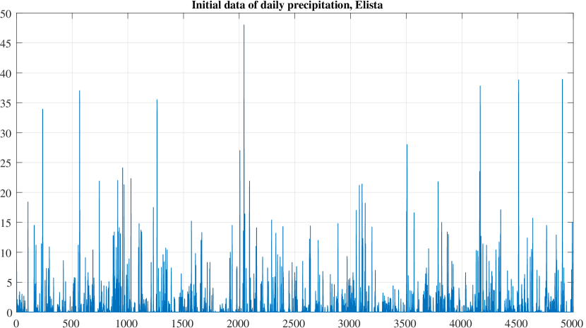
a)

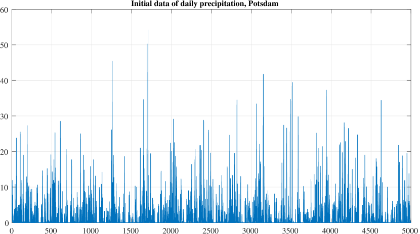
b)

Figure 1: The initial data of daily precipitation in Elista (a) and Potsdam (b).

In order to analyze the statistical regularities of the duration of wet periods this data was rearranged as shown on Figure 2a and Figure 2b.

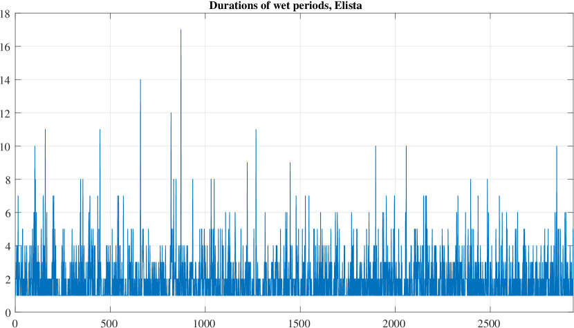
a)

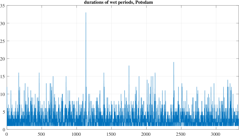
b)

Figure 2: The durations of wet periods in Elista (a) and Potsdam (b).

On these figures the horizontal axis is the number of successive wet periods. It should be mentioned that directly before and after each wet period there is at least one dry day, that is, successive wet periods are separated by dry periods. On the vertical axis there lie the durations of wet periods. In other words, the height of each “pin” on these figures is the length of the corresponding wet period measured in days and the corresponding point on the horizontal axis is the number of the wet period.

The samples of durations in both Elista and Potsdam were assumed homogeneous and independent. The best fit with these samples was demonstrated by the negative binomial distribution. Let $r>0$ and $p\in(0,1)$. We say that a random variable $Y$ has the negative binomial distribution with parameters $r$ and $p$, $Y\sim NB(r,p)$, if

$${\sf P}(Y=k)=\frac{\Gamma(r+k)}{\Gamma(r)\Gamma(k+1)}p^{r}(1-p)^{k},\quad k=0,1,2,\ldots$$

Let $X=Y+1$. Then $X\geqslant 1$ and

$${\sf P}(X=k)={\sf P}(X-1=k-1)=\frac{\Gamma(r+k-1)}{\Gamma(r)\Gamma(k-1+1)}p^{r}(1-p)^{k-1}=\frac{\Gamma(r+k-1)}{\Gamma(r)\Gamma(k)}p^{r}(1-p)^{k-1},$$

$k=1,2,3,\ldots$

Figures 3a and 3b show the histograms constructed from the corresponding samples of duration periods and the fitted negative binomial distribution. In both cases the shape parameter $r$ turned out to be less than one. For Elista $r=0.876$, $p=0.489$, for Potsdam $r=0.847$, $p=0.322$.

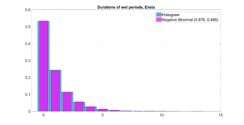
a)

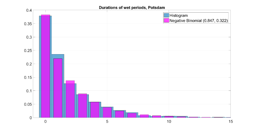
b)

Figure 3: The histogram of durations of wet periods in Elista (a) and Potsdam (b) and the fitted negative binomial distribution.

We can suggest the following explanation for the negative binomial distribution of the duration of wet periods. Each precipitation process develops in temporal and spatial coordinates. Assume that the projection of each precipitation event onto the time axis is a (random) connected set. Then attracting some rather simple, natural and well-tractable assumptions defining Poisson random measures (for example, see [4]), we come to the suggestion that, if the “temporal density” of wet days is uniform in time, then the size of each temporal projection of a precipitation event must have the Poisson distribution. But due to seasonal and other climatic trends the “temporal density” of wet days varies in a random manner. Therefore, the actual distribution of the duration of wet periods should be sought among mixed Poisson distributions. As far ago as in 1920 it was shown that the negative binomial distribution is mixed Poisson with the mixing gamma-distribution [3]: for $k=0,1,\ldots$ we have

$$\frac{1}{k!}\int_{0}^{\infty}e^{-\lambda}\lambda^{k}\frac{1}{\Gamma(r)}\Big{(}\frac{p}{1-p}\Big{)}^{r}\lambda^{r-1}\exp\Big{\{}-\frac{\lambda p}{1-p}\Big{\}}d\lambda=$$

$$\Big{(}\frac{p}{1-p}\Big{)}^{r}\frac{1}{k!\Gamma(r)}\int_{0}^{\infty}\exp\Big{\{}-\frac{\lambda}{1-p}\Big{\}}\lambda^{k+r-1}d\lambda=\frac{\Gamma(k+r)}{k!\Gamma(r)}p^{r}(1-p)^{k}.$$ (1)

In other words, if the parameter $\lambda$ of the Poisson distribution is random and has the gamma-distribution with shape parameter $r$ and scale parameter $p/(1-p)$, then the resulting mixed Poisson distribution is negative binomial with parameters $r$ and $p$.

Note that in both cases, that is, for Elista and Potsdam, the parameter $r$ of the fitted negative binomial distribution and, hence, of the mixing gamma-distribution in (1), is less than one. It is known that the gamma-distribution can be represented as a mixture of exponential laws if and only if its shape parameter is no greater than one (see [2]). In that paper it was proved that if the shape parameter $r$ of the gamma-distribution $f_{r,\theta}(x)$ satisfies the condition $0<r\leq 1$, then the gamma-density $f_{r,\theta}(x)$ can be represented as a mixed exponential distribution:

$$f_{r,\theta}(x)=\int_{0}^{\infty}p_{\theta}(\gamma)\gamma e^{-\gamma x}\,d\gamma.$$ (2)

where

$$p_{\theta}(\gamma)=\frac{(\gamma-\theta)^{-r}\theta^{r}}{\gamma\Gamma(1-r)\Gamma(r)}\mathbb{I}(\gamma\geqslant\theta).$$ (3)

But it is well known that the exponential distribution has the maximum differential entropy among all distributions concentrated on the nonnegative half-line and possessing a finite expectation. This means that the negative binomial model for the duration of wet periods has serious theoretical grounds leading to the reasoning based on the principle of non-decrease of uncertainty in closed systems. But any regional precipitation system cannot be considered as closed, it is influenced by many poorly predictable random factors. Within the mixed models (1) and (2) the distribution $p_{\theta}(\gamma)$ (3) accumulates the information concerning the statistical regularities in the integral behavior of “external” factors.

3 The analysis of the daily precipitation volumes

The distribution of daily precipitation volumes presented on Figure 4a and Figure 4b was also analyzed. It turned out that for both Elista and Potsdam data the best fit is demonstrated by the Pareto distribution defined by the distribution function

$$F_{\xi,\sigma,\mu}(x)=1-\left(1+\frac{\xi(x-\mu)}{\sigma}\right)^{-1/\xi},\quad\xi\neq 0,$$

see Figure 4a and Figure 4b.

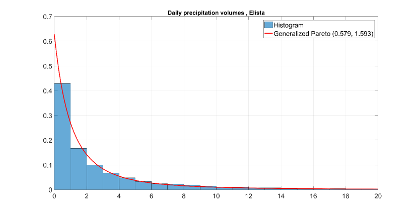
a)

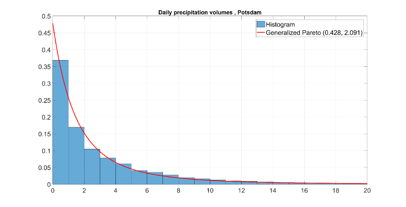
b)

Figure 4: The histogram of daily precipitation volumes in Elista (a) and Potsdam (b) and the fitted Pareto distribution.

As concerns the Pareto distribution, it can be easily seen that scale mixtures of gamma-distributions with the mixing law also having the gamma-distribution are Pareto-type distributions. Indeed, we have

$$\int_{0}^{\infty}\lambda e^{-\lambda x}\frac{\mu^{s}}{\Gamma(s)}\lambda^{s-1}e^{-\mu\lambda}d\lambda=\frac{s\mu^{s}}{(x+\mu)^{1+s}},\ \ \ x>0,$$

that is, the Pareto distribution with the density

$$p(x;s,\mu)=s\mu^{s}(x+\mu)^{-(1+s)},\ \ \ \ x>0,$$

for any $s>0$, $\mu>0$ is a mixed exponential distribution.

Moreover, a more general result can be easily proved: all scale mixtures of gamma-distributions with the mixing law also having the gamma-distribution are Pareto-type distributions. Indeed, we have

$$\frac{x^{r-1}}{\Gamma(r)}\int_{0}^{\infty}\lambda^{r}e^{-\lambda x}\frac{\mu^{s}}{\Gamma(s)}\lambda^{s-1}e^{-\mu\lambda}d\lambda=\frac{x^{r-1}\mu^{s}}{\Gamma(r)\Gamma(s)}\int_{0}^{\infty}\lambda^{r+s-1}e^{-\lambda(x+\mu)}d\lambda=$$

$$=\frac{x^{r-1}\mu^{s}}{\Gamma(r)\Gamma(s)(x+\mu)^{r+s}}\int_{0}^{\infty}(x+\mu)^{r+s-1}\lambda^{r+s-1}e^{-\lambda(x+\mu)}d\lambda(x+\mu)=\frac{\Gamma(r+s)\mu^{s}}{\Gamma(r)\Gamma(s)}\frac{x^{r-1}}{(x+\mu)^{r+s}},\ \ \ x>0.$$

And if here the shape parameter $s$ of the mixing gamma-distribution satisfies the condition $s\leqslant 1$, then from the abovesaid it follows that such Pareto distributions are also mixed exponential so that the reasoning presented in the final part of the preceding section can be applied to the daily precipitation volumes.

We also propose some similar mixture-type models for other characteristics of precipitation process, such as total precipitation volume during a wet period, etc.

References

- [1] O. Zolina, C. Simmer, K. Belyaev, S. Gulev, and P. Koltermann, Journal of Climate 26, 2022–2047 (2013).
- [2] L. J. Gleser, The American Statistician 43(2), 115–117 (1989).
- [3] M. Greenwood, and G. U. Yule, Journal of the Royal Statistical Society 83, 255–279 (1920).
- [4] J. F. C. Kingman, Poisson processes, Clarendon Press, Oxford, 1993.